WEAP Model Development WEAP Model Development for Hydrologic Region for Hydrologic Region

DemandsDemands

Mohammad Mohammad RayejRayej, Ph.D., P.E., Ph.D., P.E.Senior Engineer, W.R.Senior Engineer, W.R.

California Dept of Water ResourcesCalifornia Dept of Water Resources

WEAPWEAP• Water Evaluation And Planning Model• High level screening tool• Demand & Supply in a single tool• Demand driven water supply allocation model• Demand priorities and supply preferences• Highly scaleable in space & time• Steps through time to simulate future conditions• Very suitable to build and study future water scenarios

as affected by population, socio_economic factors and climate change

• Explore management strategies (demand reduction, supply augmentation)

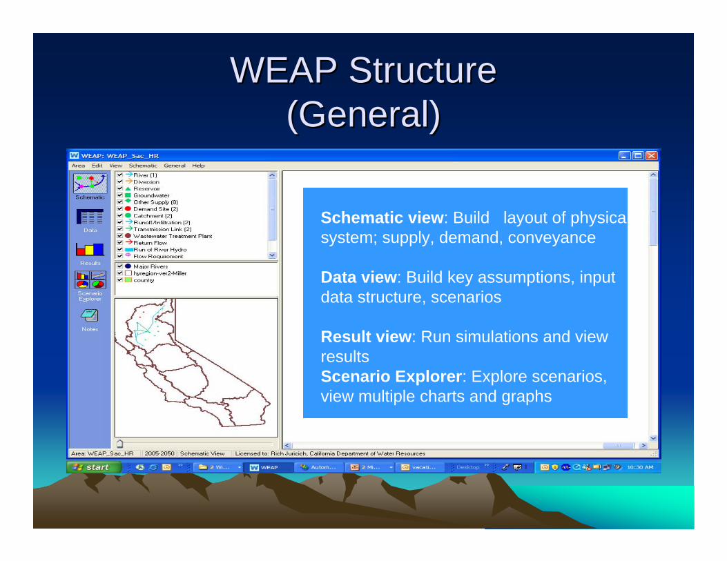
WEAP StructureWEAP Structure(General)(General)

Schematic view: Build layout of physical system; supply, demand, conveyance

Data view: Build key assumptions, input data structure, scenarios

Result view: Run simulations and view resultsScenario Explorer: Explore scenarios, view multiple charts and graphs

California Water PlanCalifornia Water Plan’’ 0909(General Assumptions)(General Assumptions)

• Base year: 2005• Projection year: 2050• Time scale: monthly time step• Space scale: Hydrologic Region• Regions not linked• High level representation of Regions

(actual water system; reservoir operations not modeled)

Applied to 10 Hydrologic Regions Applied to 10 Hydrologic Regions

• 1- North Coast• 2- San Francisco Bay• 3- Central Coast• 4- South Coast• 5- Sacramento River • 6- San Joaquin River• 7- Tulare Lake• 8- North Lahontan• 9- South Lahontan• 10- Colorado River

WEAP Schematic viewWEAP Schematic view(10 hydrologic Regions)(10 hydrologic Regions)

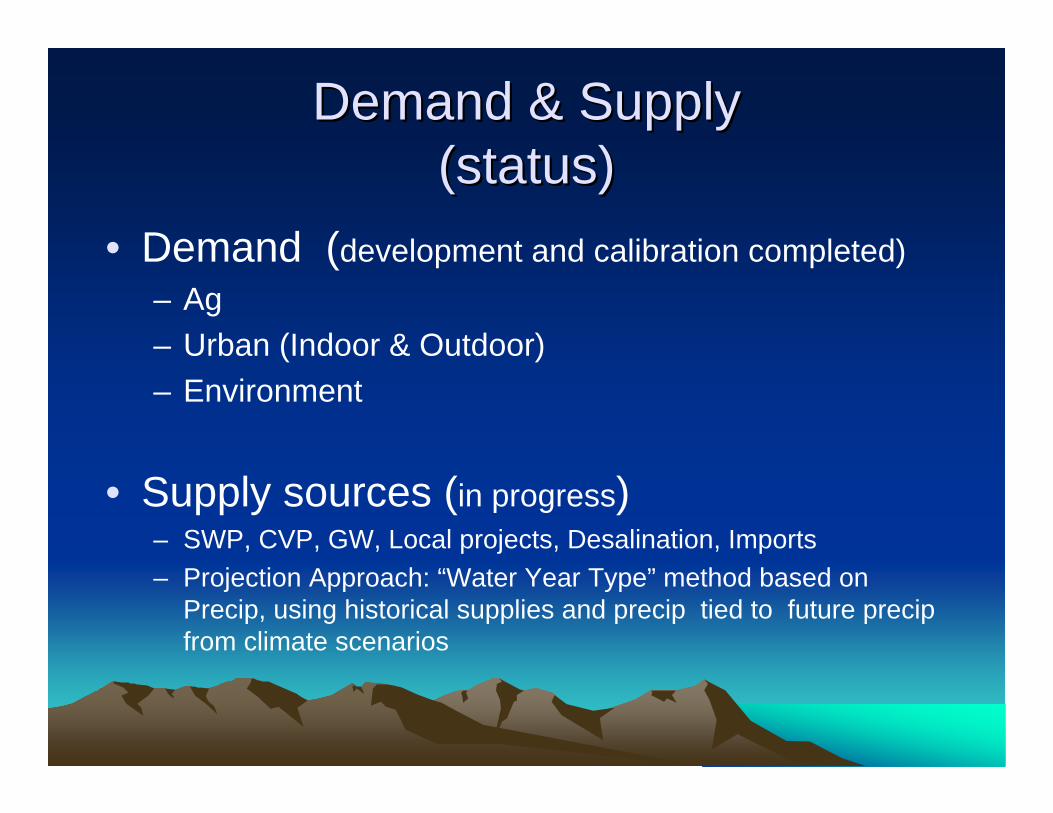
Demand & SupplyDemand & Supply(status)(status)

• Demand (development and calibration completed)– Ag– Urban (Indoor & Outdoor)– Environment

• Supply sources (in progress)– SWP, CVP, GW, Local projects, Desalination, Imports– Projection Approach: “Water Year Type” method based on

Precip, using historical supplies and precip tied to future precipfrom climate scenarios

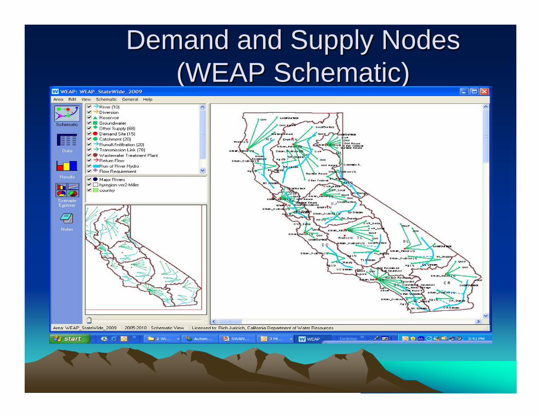
Demand and Supply Nodes Demand and Supply Nodes (WEAP Schematic) (WEAP Schematic)

SR RegionSR Region(close up)(close up)

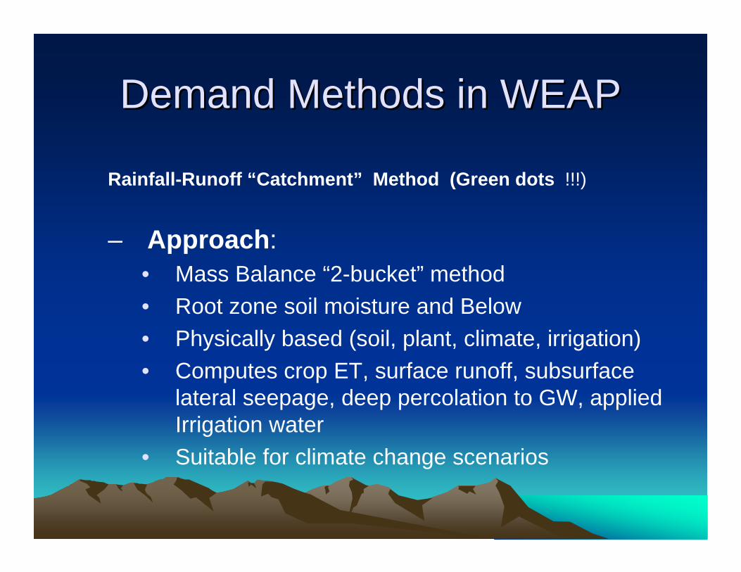
Demand Methods in WEAPDemand Methods in WEAP

Rainfall-Runoff “Catchment” Method (Green dots !!!)

– Approach:• Mass Balance “2-bucket” method• Root zone soil moisture and Below• Physically based (soil, plant, climate, irrigation)• Computes crop ET, surface runoff, subsurface

lateral seepage, deep percolation to GW, applied Irrigation water

• Suitable for climate change scenarios

Demand Methods (contDemand Methods (cont’’d)d)

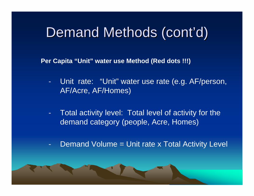
Per Capita “Unit” water use Method (Red dots !!!)

- Unit rate: “Unit” water use rate (e.g. AF/person, AF/Acre, AF/Homes)

- Total activity level: Total level of activity for the demand category (people, Acre, Homes)

- Demand Volume = Unit rate x Total Activity Level

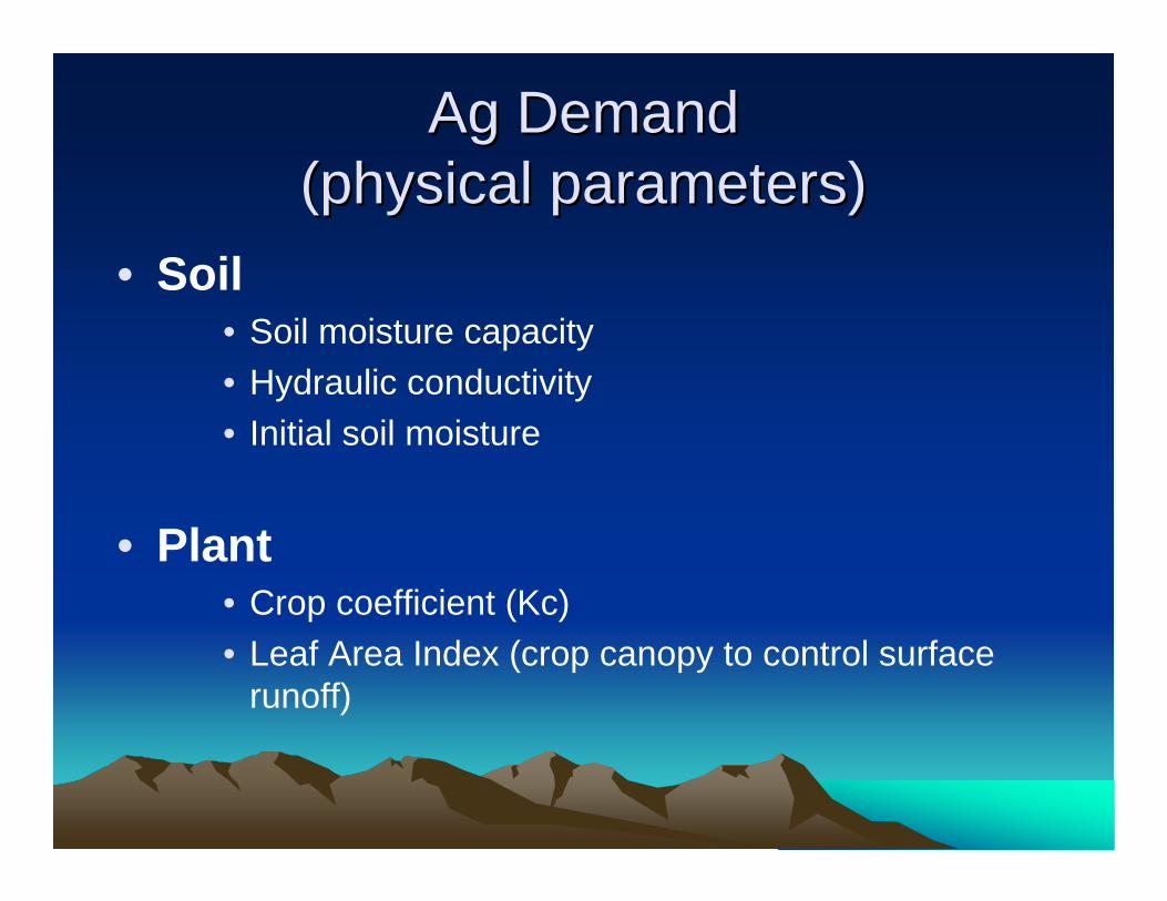
Ag DemandAg Demand(physical parameters)(physical parameters)

• Soil• Soil moisture capacity• Hydraulic conductivity• Initial soil moisture

• Plant• Crop coefficient (Kc)• Leaf Area Index (crop canopy to control surface

runoff)

WEAP data viewWEAP data view(Ag physical parameters)(Ag physical parameters)

Ag DemandAg Demand(physical parameters)(physical parameters)

• Climate• Precip• Temp• Relative Humidity• Wind Speed• Lattitude• Melting point temp (snowmelt runoff)• Freezing point temp (snowpack accumulation)

• Irrigation• Lower soil moisture Threshold (LT) (to start irrigation)• Upper soil moisture Threshold (UT) (to stop irrigation)

WEAP data viewWEAP data view(Ag climate parameters)(Ag climate parameters)

Demand Demand (Method & (Method & DisaggergationDisaggergation))

• Ag (Hydrologic catchment method)– Disaggregation (20 crop categories)

• Grain - Processing Tomato• Rice - Fresh Tomato• Cotton - Cucurbits• SugarBeet - Onion/Garlic• Corn - Potato• DryBean - OherTruck• Safflower - Almond/Pistachio• Otherfield - OtherDeciduous• Alfalfa - Subtropical• Pasture - Vine

WEAP data viewWEAP data view(Ag 20 crops (Ag 20 crops disaggregationdisaggregation))

DemandDemand(Method & (Method & DisaggregationDisaggregation))

• Urban – Urban Indoor (Per Capita) - Urban Outdoor (Catchment)

• Single Family - Single Family• Multi Family - Multi family• Commercial - Commercial• Industrial - Large landscape

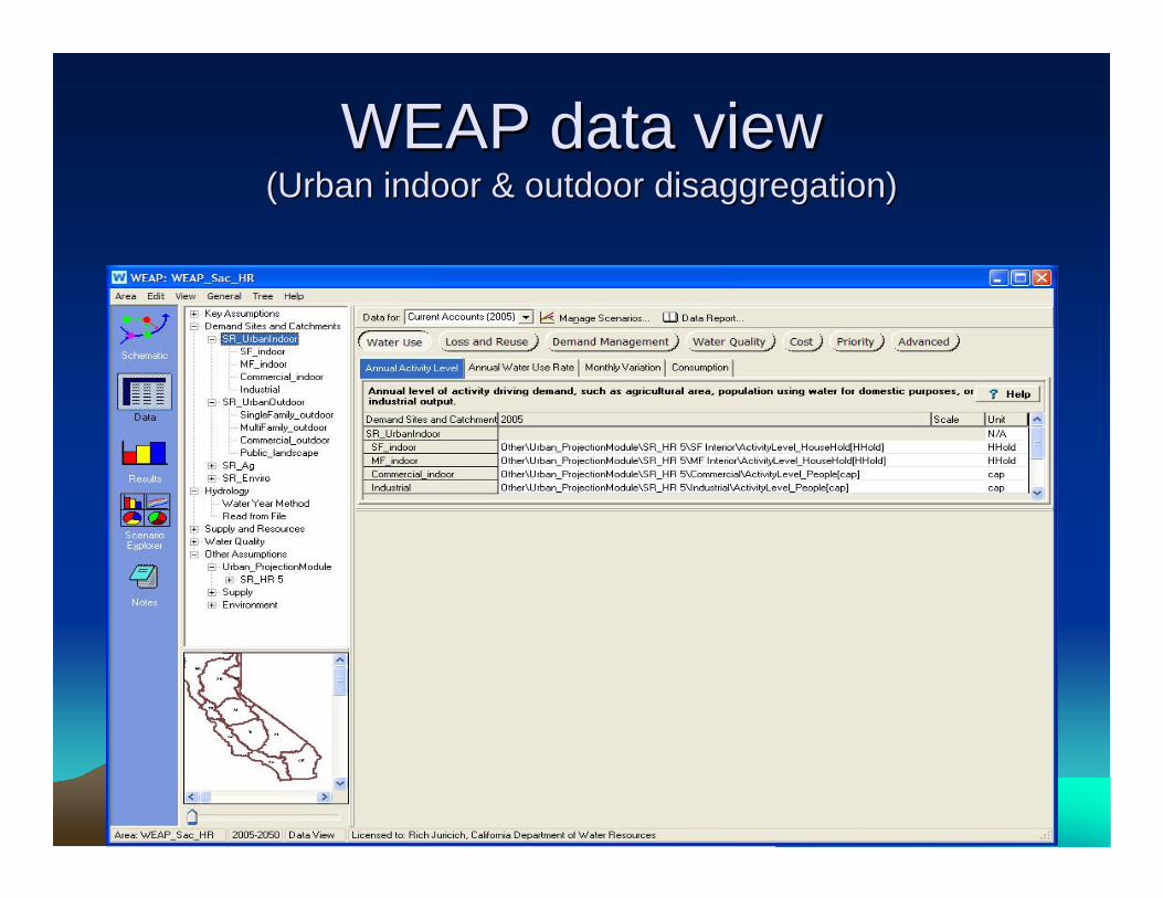
WEAP data viewWEAP data view(Urban indoor & outdoor (Urban indoor & outdoor disaggregationdisaggregation))

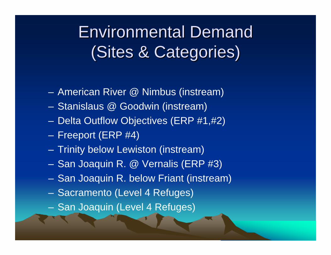
Environmental DemandEnvironmental Demand(Sites & Categories)(Sites & Categories)

– American River @ Nimbus (instream)– Stanislaus @ Goodwin (instream)– Delta Outflow Objectives (ERP #1,#2)– Freeport (ERP #4)– Trinity below Lewiston (instream)– San Joaquin R. @ Vernalis (ERP #3)– San Joaquin R. below Friant (instream)– Sacramento (Level 4 Refuges)– San Joaquin (Level 4 Refuges)

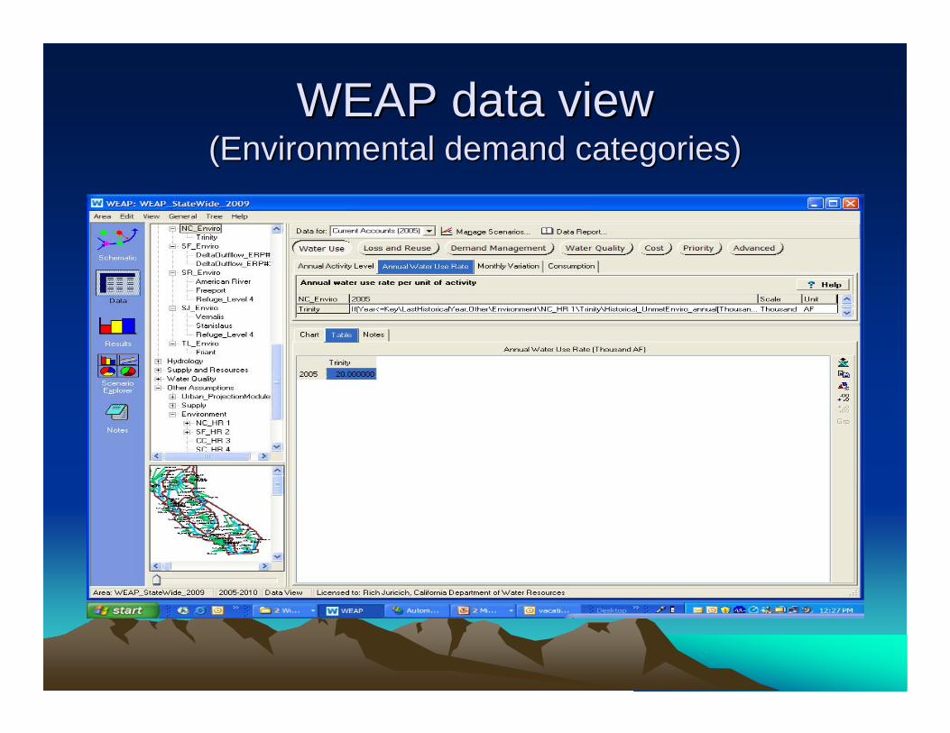
WEAP data viewWEAP data view(Environmental demand categories)(Environmental demand categories)

Demand ScenariosDemand Scenarios(General)(General)

• 3 narrative scenarios

– Driven by 3 population scenarios:

1- Current Trend Scenario – Current trend of population growth projected by DOF

2- BluePrint Scenario– Low population growth projection by PPIC

3- Expansive Scenario– High population growth projection by PPIC

• 12 Climate Scenarios– Based on 2 emission scenarios (A2 and B1) projections in Governer’s

report simulated by 6 GCM models.

WEAP ScenariosWEAP Scenarios(scenario manager)(scenario manager)

Ag Demand Ag Demand (Scenario Drivers)(Scenario Drivers)

• Population – 3 population scenarios driving Ag land use

(acre)

• Climate– 12 climate scenarios driving “unit” water use

rates (ft)

Urban Demand Urban Demand (Scenario Drivers)(Scenario Drivers)

• Urban – 3 narrative scenarios

• Population• Single Family homes• Multi Family homes• Commercial employees• Industrial employees

– Elasticity factors• Price of water• Average household income• Number of people in SF homes (Indoor demand only)• Number of people in MF homes (Indoor demand only)• Naturally Occurring conservation

– Climate (Outdoor demand only)

WEAP data viewWEAP data view(Elasticity factors)(Elasticity factors)

Ag Demand ProjectionAg Demand Projection

• Ag land use projection (2005-2050):– Based on 3 Statewide population scenarios, future Ag land decline was linearly projected

over time and proportioned into 10 regions and further divided among 20 individual crops using a low value, high value and multi_crop ratio scheme (Tom Hawkins)

– No economic factors, crop yield, international market were considered.

• Ag crop coefficients (Kc) for 20 crop categories were provided by Morteza Orangusing SIMETAW model. Kc(s) and other physical parameters were held constant over time.

• Climate data projection on Ag lands (2005-2050):– Climate data projections for 12 climate scenarios, downscaled to regional level for monthly

time-step in WEAP (precip, temp, RH and Wind Speed) were provided by David Yates (NCAR), Boulder, Colorado.

• Ag demand projection (2005-2050): – Ag land projection from above, in conjunction with climate projection, were used in WEAP

“catchment” module to give climate driven future Ag demands; total of 3 X 12 = 36 projections.

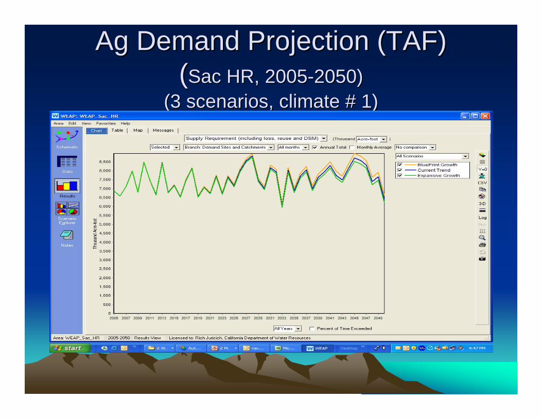
Ag Demand Projection (TAF)Ag Demand Projection (TAF)((Sac HR, 2005Sac HR, 2005--2050)2050)

(3 scenarios, climate # 1)(3 scenarios, climate # 1)

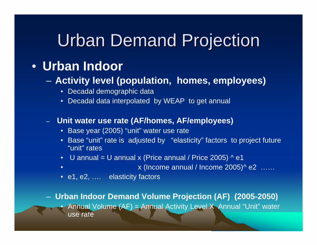
Urban Demand Projection Urban Demand Projection • Urban Indoor

– Activity level (population, homes, employees)• Decadal demographic data • Decadal data interpolated by WEAP to get annual

– Unit water use rate (AF/homes, AF/employees)• Base year (2005) “unit” water use rate• Base “unit” rate is adjusted by “elasticity” factors to project future

“unit” rates• U annual = U annual x (Price annual / Price 2005) ^ e1 • x (Income annual / Income 2005)^ e2 ……• e1, e2, …. elasticity factors

– Urban Indoor Demand Volume Projection (AF) (2005-2050)• Annual Volume (AF) = Annual Activity Level X Annual “Unit” water

use rate

Urban Indoor Demand Projection (TAF)Urban Indoor Demand Projection (TAF)(Sac HR, 2005(Sac HR, 2005--2050)2050)

(3 scenarios)(3 scenarios)

Urban Demand ProjectionUrban Demand Projection

• Urban Outdoor

• Outdoor land use projection (2005-2050)

– Historical outdoor land use (WY 2000) was used to find “Unit” value– “Unit” acre 2000 = Acres 2000 / homes 2000– Future demographics used to drive annual outdoor land use projections– Annual acre = (unit acre 2000) x (annual homes / homes 2000)

• Crop coefficients (Kc) for cool season/warm season outdoor plants were used in each region

• Climate data projection on Urban outdoor (2005-2050)– Like Ag land climate projection, the 12 future climate projection on Urban areas downscaled

on the 10 hydrologic regions were provided by David Yates (NCAR)

• Urban Outdoor Demand Projection (2005-2050)– With future Urban outdoor land use driven by 3 demographic projections, and Kc for

urban outdoor and Urban area climates under 12 climate scenarios, the “Cathment” module in WEAP is used to project future Urban outdoor demand.

Urban Outdoor Demand Projection (TAF)Urban Outdoor Demand Projection (TAF)(Sac HR, 2005(Sac HR, 2005--2050)2050)

(3 scenarios, climate #1)(3 scenarios, climate #1)

Environmental Demand Projection Environmental Demand Projection (Approach)(Approach)

• Historical “unmet” demand– Historical “actual” applied water data (1998-2007) was compared with

environmental Objectives to determine “unmet” demand.– Percentiles were applied to historical precipitations (1900-2005) for the

region to develop “Year Type” classifications, e.g. (<min=critical, 25%=Dry, 50%=Below Normal, 75%=Above Normal, >75%= Wet)

– By comparing historical “unmet” demand years with precip based “Year Type” classes above, a Year Type class was developed for each historical unmet demands.

– Within each unmet demand “Year Type” class, “min”, “avg”, “max”unmet demand values were used to assign to 3 narrative Expansive, Current Trend and BluePrint scenarios, respectively. This was to ensure the Expansive growth would result in lower future “additional desired”flow needed for environment than under BluePrint growth scenario.

Environmental Demand Projection Environmental Demand Projection (Approach)(Approach)

• Future “additional desired” flow– Then, future annual precip data (2005-2050)

for the same region was used to generate future “Year Type” classifications using the same percentiles.

– Finally, future annual “Precip” Year Type, was matched with historical “Unmet” demand Year Type class to find corresponding “additional desired flow” in respective future years when WEAP steps through time (2005-2050)

Environmental Demand Projection Environmental Demand Projection (additional desired flow, TAF, 2005(additional desired flow, TAF, 2005--2050)2050)

(Sac HR, 3 scenarios, climate #1)(Sac HR, 3 scenarios, climate #1)

NEXT STEPSNEXT STEPS

• Supply sources • Supply scenarios• Supply projections• Linkage to demand sites• Simultaneous Supply-Demand projections• Evaluation of different management

strategies (supply augmentations, demand reductions)