1

Weather routing of motorsailers

Daan Sparreboom , Mark Leslie Miller

August 2012

1 Introduction Weather routing can be described as the process of finding a route between a departure and

destination point in such a way that a chosen objective is optimized while taking into account effects

of the environment. These effects include wind, waves and current. The chosen objective for

instance can be cost, time, fuel consumption or a measure of comfort or safety.

There is a close correlation between a ship’s performance and the environment it sails in. Even more

so when the ship is (partly) propelled by wind. This is the case for sailing ships, but also for ships with

kites and Flettner rotors [Enercon E-ship]. Weather routing is therefore very important for the design

and operation of these kinds of ships. One application is the Ecoliner, a concept design for a 4 mast

dynarig multipurpose cargo ship currently in design at Dykstra Naval Architects [DNA] and an

initiative of Fairtransport [Fairtransport], see figure 1. More information about the Ecoliner can be

found in [Nikkels]. Another application is Rainbow Warrior III [Rainbow Warrior III], the Green peace

flagship with a staysail schooner rig.

Figure 1: The Ecoliner concept design [DNA]

Wind propulsion is used to reduce fuel consumption. However, in order to keep a schedule, this can

be combined with the use of an engine. This complicates the routing process since it introduces an

extra degree of freedom to the optimization: the engine setting. When only sails are used, the speed

depends solely on the chosen course; this is one degree of freedom. When an engine is also used,

both course and engine setting can be chosen.

The extra cost of a ship equipped for wind propulsion must be related to the savings in fuel it

realizes. The main question raised when presenting a design of a sail assisted cargo ship is: ‘how

much fuel can be saved by using sails?’ This research focuses on weather routing of ships that are

propelled by both wind propulsion and an engine, here called motorsailers for brevity. By using

routing simulations for the intended operating track, an estimate of the fuel consumption can be

made and the question of how much fuel is saved by installing a wind propulsion rig can be

answered.

2

2 Research goal The main goal of this research is to apply weather routing to the design process of motorsailers.

Since the goal of using sails is to save fuel in cargo shipping, fuel consumption is an important design

property. Another design property is the duration of a crossing since the transport capacity and

therefore the income depend on the time needed for a crossing. The main goal can be split up into

the following sub goals:

- Creating a model of the ship to calculate ship performance under various circumstances - Finding a routing algorithm that can optimize routes for both time and fuel consumption - Applying the methods to the evaluation of a motorsailer design

In order for a routing algorithm to find possible routes, the ship’s speed and fuel consumption must

be known. These parameters must be calculated for all admissible values of control parameters and

external parameters.

The current methods and programs are unfit for routing of motorsailers [Sparreboom] [Motte]. This

research aims to fill that gap and find a method that can be used for the routing of motorsailers with

a variable engine setting.

To illustrate the methods derived and to show their relevance and possibilities, routing is used as a

design tool for the design of the Ecoliner. By doing this, an answer can be given to the question: ‘How

much fuel can be saved by using sails on a cargo ship?’

3 Modeling the ship performance Since this research focuses on optimizing time and fuel consumption, the ship speed and fuel

consumption rate are the most important performance parameters. In order to calculate the ship

performance in various circumstances, a velocity prediction program (VPP) is used. The VPP

described here is based on data on the hull, sails and engine. These data can be obtained from model

experiments in the wind tunnel and towing tank, CFD calculations, full scale measurements or

empiric methods.

The VPP is very similar to the Windesign VPP [Windesign], a commercially available VPP for sailing

ships. It was chosen to build a new program in Matlab for three reasons: Windesign does not support

the modeling of an engine and propeller, independent wave conditions cannot be entered in

Windesign and a new program can be automated to produce lookup tables while manual iterations

would be needed when using Windesign for this.

The propeller is modeled as an additional longitudinal force on the hull. The pitch can be varied and

is chosen to require 85% of the engine maximum at the given engine RPM setting. The fuel

consumption is calculated from the specific fuel consumption of the engine. When the engine is

turned off, the fuel consumption only consists of the fuel consumption at the hotel load and the

propeller causes drag.

The added resistance in waves is calculated by using the significant wave height and mean period in a

Bretschneider spectrum. Together with the hull’s RAO for added resistance in waves and the mean

wave angle the added resistance in waves can be calculated for head to beam waves using strip

theory.

3

The most important simplifications made in the ship model are:

- Steady state presumption - No drag due to rudder angle is present and the total yawing moment is presumed zero - Following waves have no effect on the time-average ship response - Leeway is small enough to assume sin(λ)=0 and cos(λ)=1

The calculation time for one set of conditions is in the order of 0.2 seconds which is too much for

direct use in a routing algorithm. For this reason, the ship performance must be calculated previous

to the routing algorithm for various conditions. By presenting these data in a lookup table, the

routing algorithm can quickly find the ship performance. The variables influencing the ship

performance are:

- Engine setting - Wind speed and angle - Significant wave height, mean wave period and mean wave angle - Current speed and angle

To create a lookup table with these eight dimensions at a high resolution will require too much

computer memory which makes this option infeasible. Consequently, the method chosen here is to

use wind polars for multiple engine settings for finding the ship’s speed at given true wind speed and

-angle. The wind polars are corrected for leeway and velocity made good.

The effect of waves is incorporated by using a factor on the speed. This factor depends on the

significant wave height, mean wave period and wave angle. These factors will be included in a so

called wave polar. The speed change not only depends on the wave parameters, so this is a

simplification. It also depends on effects on the sails, hull and propeller by the speed change itself.

However, to limit the number of dimensions in the speed polar, a wave polar is a good option.

4 Routing using Maxsea Time Zero Maxsea Time zero (T0) is a commercially available routing program intended mainly for sailing yachts

and other sailing vessels [Maxsea]. In order to use T0 for routing of motorsailers, a minimum sailing

speed is used. Routing with a minimum speed simulates using the engine when the wind is

insufficient to reach the selected minimum speed. This ensures that the engine power is used

efficiently. The idea was introduced in [Dijkstra].

Routing simulations are performed for multiple wind polars with different minimum speeds of 0, 6, 8,

10 and 12 knots. For each minimum speed a routing is performed and the results of these are used

for calculation of the fuel consumption. The T0 routing output is combined with information on the

ship to obtain the required propeller force. The speed through the water, true wind speed and angle,

current speed and direction and sail set are used. From the required propeller force, the fuel

consumption can be calculated from propeller and engine information.

The chosen route is a crossing of the Atlantic from east to west. The weather information is obtained

from a GRIB file with an acceptable spatial resolution of 1 degree. The time step is set at 6 hours. The

maximum acceptable wind speed is set at 125 knots and the maximum wave height is at 20 meters.

4

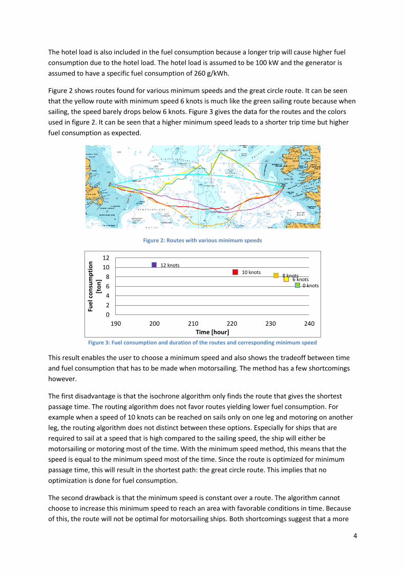
The hotel load is also included in the fuel consumption because a longer trip will cause higher fuel

consumption due to the hotel load. The hotel load is assumed to be 100 kW and the generator is

assumed to have a specific fuel consumption of 260 g/kWh.

Figure 2 shows routes found for various minimum speeds and the great circle route. It can be seen

that the yellow route with minimum speed 6 knots is much like the green sailing route because when

sailing, the speed barely drops below 6 knots. Figure 3 gives the data for the routes and the colors

used in figure 2. It can be seen that a higher minimum speed leads to a shorter trip time but higher

fuel consumption as expected.

Figure 2: Routes with various minimum speeds

Figure 3: Fuel consumption and duration of the routes and corresponding minimum speed

This result enables the user to choose a minimum speed and also shows the tradeoff between time

and fuel consumption that has to be made when motorsailing. The method has a few shortcomings

however.

The first disadvantage is that the isochrone algorithm only finds the route that gives the shortest

passage time. The routing algorithm does not favor routes yielding lower fuel consumption. For

example when a speed of 10 knots can be reached on sails only on one leg and motoring on another

leg, the routing algorithm does not distinct between these options. Especially for ships that are

required to sail at a speed that is high compared to the sailing speed, the ship will either be

motorsailing or motoring most of the time. With the minimum speed method, this means that the

speed is equal to the minimum speed most of the time. Since the route is optimized for minimum

passage time, this will result in the shortest path: the great circle route. This implies that no

optimization is done for fuel consumption.

The second drawback is that the minimum speed is constant over a route. The algorithm cannot

choose to increase this minimum speed to reach an area with favorable conditions in time. Because

of this, the route will not be optimal for motorsailing ships. Both shortcomings suggest that a more

0 knots 6 knots

8 knots 10 knots

12 knots

0

2

4

6

8

10

12

190 200 210 220 230 240

Fue

l co

nsu

mp

tio

n

[to

n]

Time [hour]

5

elaborate way to operate the engine setting is needed to perform weather routing for motorsailers.

A method to deal with this is discussed next.

5 New routing algorithm for motorsailers It was concluded that routing of motorsailers requires optimization of the fuel consumption.

However, the trip duration must also be taken into account. Therefore, a routing algorithm is

designed to optimize both fuel consumption and duration. The goal is to find multiple optimal routes

with various combinations of duration and fuel consumption. Also, the engine setting is varied along

the route. This means that the minimum speed polars and Maxsea T0 are no longer used.

5.1 Algorithm setup

The algorithm is intended for ship design purposes. No attempt is made to produce a routing

program that can be used in a user friendly way. The purpose is solely to construct an algorithm and

illustrate its use in weather routing as a design tool. This tool is called DD routing (Dykstra and Daan).

Optimization- and control variables

The optimization variables are the fuel consumption and required passage time. The first control

variable is the course of the ship. The second control variable can be either ship speed or engine

setting. When ship speed is used, the fuel consumption is calculated for the speed chosen. The speed

is chosen by the routing algorithm and must be at least the sailing speed. When engine setting is the

second control variable, the fuel consumption is known and the ship speed must be in a polar for

each possible engine setting. Using the engine setting is a more straightforward method and is

therefore chosen.

Grid choice

For creating routes, a grid is used. This discretization can be done on the basis of either time or

space. When a discretization of time is chosen, a grid can be constructed by isochrones which

depend on the ship speed. Another option is a fixed grid in space, with predefined points between

which the ship can sail. An advantage of the isochrone method is that the ship sails a course for a

fixed time and then changes course which is the way ships are operated in reality. For a fixed grid,

the time between course changes is different each leg. Another advantage of the isochrone method

over a fixed grid is that the differences between the courses that the algorithm can choose are

constant. When a rectangular fixed grid is used, the difference between the courses to the next

column of points is different for each set of two points. This causes a lower resolution for choosing

courses.

The large advantage of a fixed grid is that many calculations can be performed before actually

starting the algorithm. The weather information for example can be interpolated at each grid point at

all points in time in the GRIB file. The isochrone method is required to interpolate weather

information in space for each new location reached because the location is not known prior to the

start of the algorithm. Additionally, using a rectangular grid, the location can be indicated by indices.

This is faster than indicating the location by latitude and longitude and calculating these for each

point as required using the isochrone method. For these reasons, it is chosen to use a rectangular

grid for calculation speed and to simplify the algorithm.

6

Grid construction

The grid is constructed using the great circle between start and end. Points are distributed uniformly

across this great circle and great circles are drawn perpendicular to the initial great circle at each

point. By evenly distributing grid points on these great circles, a grid is constructed; see figure 4.

Figure 4: Fixed grid for routing around the great circle route

The ship can sail between points in the grid. The courses and distances between all allowed sets of

points are calculated prior to the actual routing algorithm using rhumb lines. If a great circle track

would be used instead, the course would change a little in one leg. This is not desirable in the

algorithm since it complicates finding the wind angle for example. Moreover, in operation a constant

course is more convenient than a great circle.

An optimal route can deviate considerably from the great circle route. This depends on the weather

conditions and on how much the ship speed depends on the weather. The size of the grid in the

direction perpendicular to the great circle determines whether it is possible for the ship to sail far

from the great circle. When the great circle distance between start and end points is larger, the

distance an optimal route may lie from the great circle can also become larger. For this reason, the

size of the grid in this direction is defined by a grid aspect ratio.

GRIB files

The information from the GRIB files used is:

- True wind direction and speed - Significant wave height of wind waves and swell combined - Mean wave period of the primary waves - Mean wave direction of the primary waves - Ocean current speed and direction

Tidal currents are neglected because of their periodic nature and also due to the fact that the

method is intended for offshore use where tidal currents have a small impact compared to effects of

wind and waves.

Number of calculations

To use a brute force calculation (i.e. calculate all possible routes with all possible engine settings)

yields an unacceptably high number of calculations. However, the current methods available for

routing cannot handle two control variables, therefore it is attempted to create a routing algorithm

similar to the brute force calculation but with a smaller number of calculations than m

NEnn for an

n by m grid and nNE engine settings. With a grid of 20*30 and 5 engine settings (quite coarse), this

would yield 1x1060 calculations.

7

The number of calculations is raised most by the exponential growth. The reason for the exponential

growth is that each point can be reached by many routes. Since each route can arrive at a point at a

different time, each route splits into NEnn new routes. If the number of routes to a point could

be limited to nR, the number of routes through the grid would be RNE nnn

, in the example above,

this would equal 3 x103 calculations. The question now, is how to reduce the number of routes to a

point that are used to continue along the grid. Evidently, when the time at which a route reaches a

point exceeds the maximum set time, it is excluded. The same goes for fuel consumption. More

importantly, by considering the choice between fuel consumption and duration that has to be made

in routing of motorsailers, the following method can also be applied.

If two routes arrive at the same point at the same time, but route A needs more fuel than route B,

route A can never be part of an optimal route. Also, when route A arrives at the point later and by

using more fuel than route B, route A can be excluded too. These considerations result in the notion

that routes to a point can be excluded when they are not part of a Pareto front. This is illustrated in

figure 5 where the green points constitute the Pareto front of all possible points, shown in blue. The

red circles show nR selected points at equally spaced intervals to continue with.

Figure 5: Illustration of the method to exclude routes using a Pareto front

In order to further decrease calculation time, the courses the algorithm can choose are restricted by

a course range. This method is sensible since it is very unlikely that a ship will make very large course

alternations on an optimal route.

Speed calculation

Wind polars give the ship speed for a number of true wind speeds and angles. The calm water

boatspeed is interpolated in the polars, based on the true wind data from the GRIB file. The same

method is applied to the wave polar which is interpolated for significant wave height, mean period

and mean angle.

Each leg is “sailed” with all chosen engine settings. When the ship speed in calm water is known, the

factor for the speed in waves is applied. First the wave angle is calculated from the wave direction

and the course in the same way as the wind angle. Then, the factor on the speed in waves is found by

finding the value corresponding to this wave angle. The current is incorporated in the true wind and

in the speed over ground.

0

2

4

6

8

10

12

35 40 45 50 55 60 65 70

Fue

l co

nsu

mp

tio

n [

ton

]

Time [h]

All routes Paretofront After route exclusion

8

Finally, the leg duration is calculated by using the ship speed found and the leg distance. Since the

fuel consumption rate is known for the used engine setting, the fuel consumption for the leg can be

calculated from the duration and fuel consumption rate.

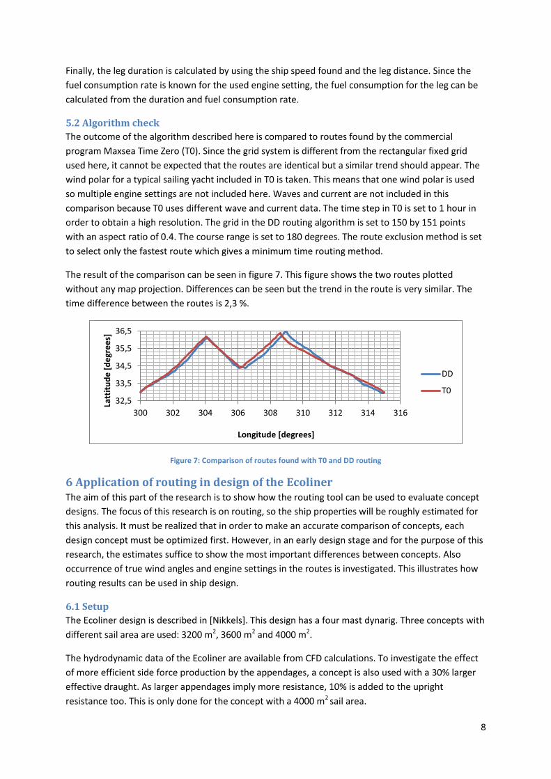
5.2 Algorithm check

The outcome of the algorithm described here is compared to routes found by the commercial

program Maxsea Time Zero (T0). Since the grid system is different from the rectangular fixed grid

used here, it cannot be expected that the routes are identical but a similar trend should appear. The

wind polar for a typical sailing yacht included in T0 is taken. This means that one wind polar is used

so multiple engine settings are not included here. Waves and current are not included in this

comparison because T0 uses different wave and current data. The time step in T0 is set to 1 hour in

order to obtain a high resolution. The grid in the DD routing algorithm is set to 150 by 151 points

with an aspect ratio of 0.4. The course range is set to 180 degrees. The route exclusion method is set

to select only the fastest route which gives a minimum time routing method.

The result of the comparison can be seen in figure 7. This figure shows the two routes plotted

without any map projection. Differences can be seen but the trend in the route is very similar. The

time difference between the routes is 2,3 %.

Figure 7: Comparison of routes found with T0 and DD routing

6 Application of routing in design of the Ecoliner The aim of this part of the research is to show how the routing tool can be used to evaluate concept

designs. The focus of this research is on routing, so the ship properties will be roughly estimated for

this analysis. It must be realized that in order to make an accurate comparison of concepts, each

design concept must be optimized first. However, in an early design stage and for the purpose of this

research, the estimates suffice to show the most important differences between concepts. Also

occurrence of true wind angles and engine settings in the routes is investigated. This illustrates how

routing results can be used in ship design.

6.1 Setup

The Ecoliner design is described in [Nikkels]. This design has a four mast dynarig. Three concepts with

different sail area are used: 3200 m2, 3600 m2 and 4000 m2.

The hydrodynamic data of the Ecoliner are available from CFD calculations. To investigate the effect

of more efficient side force production by the appendages, a concept is also used with a 30% larger

effective draught. As larger appendages imply more resistance, 10% is added to the upright

resistance too. This is only done for the concept with a 4000 m2 sail area.

32,5

33,5

34,5

35,5

36,5

300 302 304 306 308 310 312 314 316

Latt

itu

de

[d

egr

ee

s]

Longitude [degrees]

DD

T0

9

The Dynarig is also compared with Flettner rotors. Flettner rotor data from tests by the Maritime

Department of Hochschule Emden-Leer are used. These tests are done for rotors with an aspect ratio

of 4.76 with end plates. Three of these rotors are used on this concept. The aspect ratio is equal to

the aspect ratio of the tests. The length is chosen in such a way that the heeling moment is similar to

the heeling moment of the dynarig. Different rotation rates are modeled by various sail sets.

In order to account for the weight of the rig, this is subtracted from the cargo capacity which

influences the deadweight. No other changes than those described are made to the concepts. It can

be argued that a more accurate comparison can be made when the concept designs are further

developed. However, the changes described give a good impression in an early design stage and

suffice to illustrate the application of the routing tool in the design.

The costs of operating a ship can be used to choose the ship speed. Also a comparison between

designs can be made using costs. How this is done will be described in the next paragraph. Here the

cost calculation is explained. Similar to the ship performance, the cost model is estimated for the

purpose of illustrating the method. A more thorough study in the operating cost is needed to make a

good comparison. The operating costs constitute of fuel costs per ton of fuel and cost per time unit.

Marine diesel oil (MDO) is used as fuel for the Ecoliner. The cost of MDO in Rotterdam on 23th July

2012 is 877 $/ton [Navigate]. The ship is assumed to sail 268 days a year. Bulk carriers spend 24 days

off hire on average [Stopford]. The days spent in port and in ballast are both assumed to be 10% of

the total. The assumed number of days in ballast is low because the ship is relatively small and is

intended for a liner service.

A GRIB file archive of 2006 and 2007 with a spatial resolution of 1 degree is available, courtesy to

Peter Naaijen. The East point is 45 oN 15 oW and the West point is 45 oN 45 oW. The grid has 30 points

along the great circle route and 51 points perpendicular to it and an aspect ratio of 0.6. For 1st

January 2006, the chosen grid size results in an average leg time of 3 hours and a maximum course

difference of 19,4 o. The course deviation from the great circle course is 64,9 o so a course range of

140 o is chosen. For each start date, 15 routes are calculated. This results in an average time interval

smaller than the required 3 hours which is the time interval between weather updates.

The maximum time a route can take is set to 360 hours which is the duration of each weather file.

The maximum allowable true wind speed is set to 50 knots and the maximum significant wave height

is 10 meters. In order to simulate the ship operation, routings are performed from East to West and

vice versa.

6.2 Analyzing the results

In total, 15 routes are found for each start date. In order to compare ship concepts, a choice must be

made between these points. Here, this is done in two ways. The first method is to set the average

speed along the great circle, speeds of 10 and 12 knots are used for this. The second method is to

choose the speed with the lowest cost according to the cost model presented in this paragraph. The

first method is illustrated in figure 8. This graph shows the cost of fuel, the cost due to trip duration

and the total cost. It can be seen that the speed for minimum cost is 8,4 knots for this date.

10

Figure 8: Fuel cost, cost for trip duration and total cost for various average speeds along the great circle

6.3 Results

The total trip cost, trip fuel consumption and trip carbon dioxide emission are calculated for each

departure date and for east to west and west to east. The data averaged over all start dates are

presented in tables 1 and 2 in a comparison of all concepts to the motor only concept. Table 1 shows

the results for the current fuel price and table 2 shows the results for a fuel price increased by 20%.

All results are given per ton deadweight and distance transported. By dividing by deadweight, the

different cargo carrying capacities of the concepts are taken into consideration. Dividing the trip cost

by deadweight and distance gives the required freight rate. Figure 9 and 10 show graphs of the cost,

fuel consumption and CO2 emission over time at economical speed for the current fuel price.

Economical speed 10 knots 12 knots

Speed Cost Fuel Cost Fuel Cost Fuel

Dynarig 3200 m2 9.61 1% 45% -4% 26% -6% 14%

Dynarig 3600 m2 9.55 1% 48% -5% 25% -7% 12%

Dynarig 4000 m2 9.57 2% 51% -4% 28% -6% 14%

Dynarig 4000 m2+Te 9.50 5% 60% -1% 34% -5% 17%

Flettner rotors 9.00 -3% 52% -10% 15% -15% 2% Table 1: Savings in cost and fuel for the economical speed, 10 and 12 knots for all concepts compared to the motor

concept

Economical speed 10 knots 12 knots

Speed Cost Fuel Cost Fuel Cost Fuel

Dynarig 3200 m2 8.93 5% 53% -1% 26% -3% 14%

Dynarig 3600 m2 8.98 5% 54% -2% 25% -5% 12%

Dynarig 4000 m2 9.07 6% 55% -1% 28% -4% 14%

Dynarig 4000 m2+Te 9.02 10% 65% 2% 34% -2% 17%

Flettner rotors 8.61 2% 56% -7% 15% -13% 2% Table 2: Savings in cost and fuel for the economical speed, 10 and 12 knots for all concepts compared to the motor

concept with the fuel price increased by 20%

0

20000

40000

60000

80000

100000

120000

5 7 9 11 13

Trip

co

st [

$]

Average speed along great circle [kts]

Cost FC

Cost T

Cost sum

11

Figure 9: Cost per ton deadweight and distance for all concepts at the economic speed

Figure 10: Fuel consumption and CO2 emission per ton deadweight and distance for all concepts at the economic speed

It can be seen that at the economic speed, the cost is lower when a rig is used. For fixed speeds of 10

and 12 knots, the costs are higher for the concepts with a rig except the 4000 m2 dynarig with

increased effective draught. The fuel consumption is lower for concepts with a rig in all cases.

In order to investigate the occurrence of various true wind angles, the occurrence of true wind angles

is plotted for the routes with the lowest cost. The result can be seen in figure 11.

0,00

2,00

4,00

6,00

8,00

10,00

12,00

14,00

14-12-2005 2-7-2006 18-1-2007 6-8-2007

Co

st p

er

DW

T*D

[$

/kg*

nm

]

Date

Cost East -West

3200 EW

3600 EW

4000 EW

4000+Te EW

Flettner EW

motor EW

0

5

10

15

20

0,00

1,00

2,00

3,00

4,00

5,00

6,00

7,00

14-12-2005 2-7-2006 18-1-2007 6-8-2007

CO

2 e

mis

sio

ns

[g/t

on

*nm

]

Fue

l pe

r D

WT*

D [

g/to

n*n

m]

Date

Fuel East -West

3200 EW

3600 EW

4000 EW

4000+Te EW

Flettner EW

motor EW

12

Figure 11: Occurrence of true wind angles in least cost routes for all concepts

For some departure dates, no data are available. This is caused by the fact that some routings failed

to find a route because the wave height or the wind speed was too high. When this is the case for the

departure of destination point, the ship speed is zero and no routes are found. Especially the engine

only concept suffers from this because it uses only engine propulsion where the other concepts use

sail propulsion as well. When no route is found, the start date is discarded and has no effect on the

final result.

9 Conclusions and recommendations It can be concluded that the research goal: application of weather routing to the design process of

motorsailers is reached. It is shown how the developed methods are used to evaluate concept

designs. The savings in cost and fuel by using various rigs are shown.

More research has to be done to further investigate the effects that sails have on the propeller

performance and the added resistance in waves. This will enable a more accurate calculation of the

ship performance which is important for routing. Examples are the effect of leeway on the propeller

efficiency and the effect of heel on the added resistance in waves. Another valuable addition is a

comparison of VPP results to performance of the full size ship.

The reliability of the routing algorithm is tested by comparing output parameters to the update

period of the GRIB file. It must be noted that this comparison only answers whether the result is

reliable within the accuracy of the weather data and the interpolation. The comparison of routing

results to T0 shows good agreement for a ship with a fixed engine setting.

The result of this kind of comparison can be used when making design choices for motorsailers. For

the comparison made here, the concepts with a rig have a lower fuel consumption, especially when

sailing at economic speed. The costs for operating the ship are also lower at economic speed but

higher at average speeds of 10 and 12 knots. This information is summarized in table 1. The analysis

will be more reliable when the weather data archive spans a larger amount of time.

0,00

1,00

2,00

3,00

4,00

5,00

6,00

7,00

8,00

0 30 60 90 120 150 180

Occ

ure

nce

[%

]

TWA

3200

3600

4000

4000+Te

Flettner

motor

13

References [Dijkstra] G. Dijkstra, M. Leslie Miller, Dynamic routing for motor sailing ships and – yachts, Dykstra

Naval Architects, 2011

[DNA] http://www.gdnp.nl

[Enercon E-ship] http://www.marinebuzz.com/2008/08/08/e-ship-1-with-sailing-rotors-to-reduce-

fuel-costs-and-to-reduce-emissions/

[Fairtransport] http://fairtransport.homestead.com/

[Maxsea] http://www.maxsea.com

[Motte] R. Motte, R.S. Burns, S. Calvert, An overview of current methods used in weather routing,

Journal of Navigation (1988), 41 : pp 101-113

[Navigate] http://navigatemag.ru/bunker/

[Nikkels] T. Nikkels, T. van Es, E. Mobron, The Ecoliner concept, Dykstra Naval Architects, 2012

[Rainbow Warrior III] http://www.greenpeace.org/international/en/about/ships/the-rainbow-

warrior/

[Sparreboom] D. Sparreboom, Weather routing of motorsailers, TU Delft, August 2012

[Windesign] Windesign user’s guide version 4.0, Yacht Research International, Inc., 2003