Web Appendix to External Integration, Structural

Transformation and Economic Development:

Evidence from Argentina 1870-1914

(Not for Publication)1

Pablo Fajgelbaum2

UCLA and NBER

Stephen J. Redding3

Princeton and NBER

A.1 Introduction

This appendix contains the technical derivations of expressions reported in the paper, the proofs

of propositions and additional supplementary material. Equations in the main paper are referenced

by their number (for example (1)), while equations in this web appendix are referenced by the letter

A and their number (for example (A.1)).

A.2 Theoretical Model

A.2.1 Proofs of the Propositions

Proposition 1. There exists a unique general equilibrium.

Proof. We assume that each location is fully specialized in sector A. Similar steps apply if a location

is fully specialized in M or incompletely specialized, and Proposition 2 shows the condition for

complete specialization as function of exogenous variables.

Step 1: Solve for {r (`) , w (`) , PN (`)} using conditions (i) and (ii) from Definition 1. First,

using (ii) and (11) evaluated at i = A gives the prices as function of the wage-rental ratio,

w(`) = zA (`)! (`)↵A

,

r(`) = zA (`)! (`)↵A

�1,

PN (`) =zA (`)

zN (`)! (`)↵A

�↵N

.

1We would like to thank Princeton University and UCLA for research support. Pablo Fajgelbaum thanks theUCLA Ziman Center for Real Estate for financial support. Responsibility for results, opinions and errors is theauthors’ alone.

2Department of Economics, 8283 Bunche Hall, Los Angeles, CA 90095. Tel: 310-794-7241. Email: pfajgel-baum@gmail.com.

3Fisher Hall, Princeton University, Princeton, NJ 08544. Tel: 609 2584016. Email: reddings@princeton.edu.

57

Following the steps in 3.6 we reach expression (15), which can be written as follows:

�T

✓

u

⇤

ezA (`)! (`)↵A

◆1��

+ (1� �T )

✓

u

⇤

zN (`)! (`)↵N

◆1��

= 1. (A.1)

Given that 0 < � < 1, the expression on the left is continuous, strictly decreasing in ! (`), it goes

to 1 as ! (`) goes to 0, and it goes to 0 as ! (`) goes to 1. Therefore, there is a unique ! (`)

consistent with (15).

Step 2: Solve for all quantities in each location given prices. As a first preliminary step, we

use (11) evaluated at i = A and w (`) = u

⇤E (`) from (i) to write the ratio of the price index in the

traded sector to the total price index as follows:

ET (`)

E (`)=

! (`)�↵A

ezA (`)u

⇤, (A.2)

PN (`)

E (`)=

! (`)�↵N

zN (`)u

⇤. (A.3)

Combining (A.2) with (A.1) we obtain (33) and (34) in the text,

zN (`) = u

⇤! (`)�↵

N

1� �T

1� eET (`)

!

11��

, (A.4)

ezA (`) = u

⇤! (`)�↵

A

�T

e

ET (`)

!

11��

. (A.5)

where

e

ET (`) = �T

✓

ET

E

◆1��

.

As a second preliminary step, we solve for factor demand in the non-tradable sector. Using (A.3)

and the definition of income per unit of land, y (`) =⇣

n (`) + 1!(`)

⌘

w (`), demand for non-traded

goods in (5) is

cN (`) = (1� �T )

✓

! (`)�↵N

zNu

⇤◆�� ✓

n (`) +1

! (`)

◆

w (`) . (A.6)

In turn, from the Cobb-Douglas production function in the non-traded sector in (6) we have that

total labor and land used in the non-traded sector are

nN (`)LN (`) = (1� ↵N )cN (`)L (`)

zN (`)! (`)�↵

N

, (A.7)

LN (`) = ↵NcN (`)L (`)

zN (`)! (`) 1�↵

N

, (A.8)

where we have imposed market clearing in the non-traded sector (condition (v) of Definition (1)).

Next, we impose the land and labor market clearing conditions (condition (iii) and (iv) of

58

Definition (1)). Combining (A.6), (A.7), (A.8) for factor demands in the non-traded sector, (10)

evaluated at i = A for labor demand in sector A, and the expression for 1 � e

ET obtained from

(A.4), we reach the following system, in which conditions (iii) and (iv) of Definition (1) can be

written respectively as follows

↵N

⇣

1� eET (`)⌘

✓

n (`) +1

! (`)

◆

+�A (`)

! (`)=

1

! (`), (A.9)

(1� ↵N )⇣

1� eET (`)⌘

✓

n (`) +1

! (`)

◆

+1� ↵A

↵A

�A (`)

! (`)= n (`) , (A.10)

where �A (`) = LA (`) /L (`) is the land share in agriculture. Adding up these two equations, we

find�A (`)

! (`)= ↵A

e

ET (`)

✓

n (`) +1

! (`)

◆

.

Replacing this back in (A.9) we obtain (21) and (22) in the paper, as well as

�A (`) =e

ET (`)↵A⇣

1� eET (`)⌘

↵N + e

ET (`)↵A

.

Since we have shown that ! (`) is uniquely determined and, given ET (`), u⇤, and ! (`), so is eET (`)

from (A.2), we have constructed the unique local equilibrium given u

⇤ and the prices of tradable

goods for each location `.

Step 3: Impose no-arbitrage (condition (vi) of Definition (1)) and find the unique u

⇤ that

solves labor market clearing (condition (vii) of the equilibrium). First, combine (21) and (22) to

express population density as

n (`) =(1� ↵A) (1� ↵N )

↵N (1� ↵A) + (↵A � ↵N ) ⌫A (`)

1

!(`). (A.11)

Using (A.1) and (22), we can express the infinitesimal change in the log n (`) and ⌫A (`) as function

of the changes in ! (`) and ET

(`)E(`) :

bn (`) = � (↵A � ↵N ) ⌫A (`)

↵N (1� ↵A) + (↵A � ↵N ) ⌫A (`)b⌫A (`)� b!(`), (A.12)

b⌫A (`) =(1� ↵A) + (↵A � ↵N ) ⌫A (`)

1� ↵A(1� �)

\✓ET (`)

E (`)

◆

. (A.13)

In turn, from (A.1) and (A.2) we can express the total derivative of ln! (`) and ln⇣

ET

(`)E(`)

⌘

as (25)

59

and (26). Therefore, keeping the productivities {ezA (`) , zN (`)} constant, we obtain:

b! (`) =(1� ↵A) + (↵A � ↵N ) ⌫A (`)

↵A (1� ↵N ) ⌫A (`) + ↵N (1� ↵A) (1� ⌫A (`))c

u

⇤ (A.14)

\✓ET (`)

E (`)

◆

= � (1� ↵A) (1� ⌫A (`)) (↵A � ↵N )

↵A (1� ↵N ) ⌫A (`) + ↵N (1� ↵A) (1� ⌫A (`))c

u

⇤ (A.15)

Combining (A.12) to (A.15), we have that:

bn (`)c

u

⇤=

(1� �) (1� ⌫A (`)) (↵A � ↵N )2 ⌫A (`)

↵N (1� ↵A) + (↵A � ↵N ) ⌫A (`)� 1

!

(1� ↵A) + (↵A � ↵N ) ⌫A (`)

↵A (1� ↵N ) ⌫A (`) + ↵N (1� ↵A) (1� ⌫A (`)).

The term is brackets is negative, implying that bn(`)cu⇤ < 0. Therefore, population density is strictly

decreasing with the real wage in every location. Moreover, since ⌫A (`) 2 (0, 1) the first term in

(A.11) is bounded. Using from (A.1) that limu⇤!1 ! (`) = 1 and limu⇤!0 ! (`) = 0, this implies

that limu⇤!1 n (`) = 0 and limu⇤!0 n (`) = 1. Aggregate labor demandP

`2L L(`)n(`) inherits

these properties, implying that there is a unique u⇤ consistent with aggregate labor-market clearing

(condition (vii) of Definition (1)).

Proposition 2. If location ` trades, it is either fully specialized in Agriculture, in which case

!A (`) < !

a (`), or fully specialized in Manufacturing, in which case !M (`) < !

a (`). Complete

specialization in Agriculture occurs for su�ciently high zA (`).

Proof. If location ` trades, it takes the prices of traded goods {Pg (`)}Gg=1 , PM (`) as given. Con-

dition (ii) of Definition (1) then implies that region ` has positive output in sector j only if

j 2 argmini=A,M,N {!i (`)}. The Inada condition implies that N 2 argmini=A,M,N {!i (`)}. Hence,

if location ` has positive output in sector i = A,M , the wage-rental ratio is equals the unique !i (`)

that solves (14), which we can write

h

�T (zi (`)!i (`)↵i)��1 + (1� �T ) (zN (`)!i (`)

↵N )��1

i

1��1

= u

⇤

where zi (`) = Pi

(`)E

T

(`)zi (`) . Therefore, the location is either fully specialized in agriculture when

!A (`) < !M (`), or fully specialized in manufacturing if !M (`) < !A (`). Taking the total derivative

of !A (`) with respect to zA (`) and using (11), we have

c!A (`) = �e

ET (`)czA (`)⇣

1� eET (`)⌘

↵N + e

ET (`)↵A

< 0.

Since !M (`) is independent of zA (`), if zA (`) is su�ciently low, then !A (`) < !M (`). Additionally,

if !A (`) = !M (`), then (11) implies that both are equal to !

a (`) . Hence, if !A (`) < !M (`), then

!A (`) < !

a (`).

Proposition 3. If traded and non-traded goods are complements (� < 1) and agriculture is more

60

land-intensive than non-traded activities, (↵A > ↵N ), then high trade-cost locations (locations ` with

higher transport costs � (`, `0) and hence lower ezA (`)) have (a) higher wage-rental ratios (higher

! (`)), (b) lower relative prices of non-traded goods (higher ET (`) /E (`)), (c) lower population

densities (lower n (`)), and (d) larger shares of labor in agriculture (larger ⌫A (`)).

Proof. Equations (25) and (26) imply (a) and (b). Results (c) and (d) follow by inspection of (21)

and (22) .

Proposition 4. Reductions in external and internal trade costs that raise a location’s adjusted

agricultural productivity (bezA (`)) (a) reduce its wage-rental ratio (lower ! (`)), (b) increase its

relative price of the non-traded good (lower ET (`) /E (`)), (c) raise its population density (higher

n (`)), (d) reduce its share of labor in agriculture (lower ⌫A (`)), and hence (e) increase its urban

population share.

Proof. Equations (25) and (26) imply (a) and (b). Results (c) and (d) follow by inspection of (21)

and (22) .

A.3 Additional Theoretical Results

A.3.1 Specialization on the Extensive Margin

As mentioned in footnote 30 in the paper, if transport costs di↵er across goods and increase

with distance to ports, the model implies that more remote regions export a narrower range of

products than more centrally-located regions, because transport costs are a source of comparative

advantage.

To see this, consider a set of locations with identical technologies, Tg (`) = Tg and ✓ (`) = ✓,

and suppose that ` indexes distance to the nearest port. Then, as distance ` increases, the share

of land allocated to good g defined in (17) varies as follows:

l

0g (`)

lg (`)= ✓

P

0g(`)

Pg(`)�

GX

h=1

P

0h(`)

Ph(`)lh (`)

!

.

Assume iceberg trade costs ⌧g for each good, order goods such that ⌧1 < ⌧2 < .. < ⌧G, and suppose

that all goods are shipped internally. If the prices are determined by no-arbitrage with the port

then Pg (`) = P

⇤g e

�⌧g

` . This implies thatl0g

(`)lg

(`) > 0 ! ⌧g < ⌧g (`), where ⌧g =P

h ⌧hlh (`), i.e., as

we move inland, comparative advantages strengthen for goods with lower transportation costs and

weaken for goods with high transportation costs.

If all prices were determined by no-arbitrage with the port, we would have that ⌧g 0 (`) < 0 and

⌧g ! ⌧1. Hence, for each good g > 1 there would be a threshold `g above which its land share

is decreasing,l0g

(`)lg

(`) < 0 ! ` > `g, where `G < `G�1 < .. < `2. Each good g > 2 would not be

exported for all ` > `

⇤g > `g, where l

0g

⇣

`

⇤g

⌘

= �g, and there would be some `1 such that only g = 1

61

is exported for all ` > `1. Hence, under heterogeneous iceberg costs, the number of exported goods

decreases toward the interior and, as ` increases, goods with higher ⌧g are dropped.

A.3.2 Extended Model with Endogenous Land Use

In the model, all land is used productively. Therefore in our empirical analysis we use geo-

graphical land area as our measure of land area in the model. Here, we develop an extension of the

model in which landowners make an endogenous decision whether to leave land wild or convert it

to productive use. In this extension, the amount of land used in each location is also endogenous.

In our baseline version of the model in the paper, the zero populations observed for some

locations in the data are rationalized by zero productivities in tradables: zA (`) = zM (`) = 0. In

this extension of the model, a location may also have zero population because it is not profitable

to convert land to productive use.

Now, we use L (`) to denote the total land area of each location, and L (`) to denote the land

area that is used productively. The only extension to the baseline model is the following: each land

plot j 2 L (`) requires a fixed cost of fj units of labor to be opened and maintained for productive

use. Once opened, the specialization across sectors and goods within agriculture is the same as in

the baseline model. The cost fj is independently and identically distributed across land plots and

districts. We let Gf (x) be the share of land plots in each district whose cost f is less than x.

Conditional on a land plot being open for productive use, we can solve (8) and (9) as before.

From the solution to this problem, we obtain the expected (gross) land rents from using any land

plot j for production in sector i,

ri (`) = fi (`)w (`) ,

where fi (`) is defined identically to the inverse of !i (`) in (11). If a location is specialized in

agriculture, f (`) equals the inverse of ! (`) from (15). Net rents to the landowner of plot j are

then

rj (`) =�

f (`)� fj�

w (`) ,

where land is converted to productive use if these net rents are positive. The total amount of land

used can be expressed as:

L (`) = Gf

�

f (`)�

L (`) .

The determination of f (`) is independent from the amount of land that is used, and therefore

from the support of the fixed-cost distribution Gf (x). Therefore, as long as the support of this

distribution is bounded from below by some positive number, we will have L (`) = 0 for su�ciently

low ! (`).

While this extension does not a↵ect gross returns to land and labor (i.e., Step 1 in the proof of

Proposition 1), it does a↵ect the model prediction for population density and for the agricultural

labor and land share. Following steps similar to Step 2 in the proof of Proposition 1 we reach the

62

following solutions for (21) and (22):

n (`) =N (`)

L (`)=

1

↵N + (↵A � ↵N ) eET (`)� 1

!

f (`) + E⇥

f | f < f (`)⇤

, (A.16)

and

⌫A (`) =NA (`)

N (`)=

e

ET (`)�

↵AE⇥

f | f < f (`)⇤

+ (1� ↵A) f (`)�

⇣

↵N + e

ET (`) (↵A � ↵N )⌘

�

E⇥

f | f < f (`)⇤

� f (`)�

+ f (`). (A.17)

where eET (`) ⌘ �T

⇣

ET

(`)E(`)

⌘1��. It can be verified that these expressions nest (21) and (22) for the

case without fixed costs, in which E⇥

f | f < f (`)⇤

= 0.

A.4 Additional Empirical Results

In this section of the appendix, we report additional empirical results discussed in the main

paper. Figures 3-5 of the paper show the evolution of the spatial distribution of population in 1869,

1895 and 1914. Figures 13-15 in this web appendix show the evolution of the spatial distribution of

urban population shares over time. As shown in Figure 13, high urban population shares in 1869

were concentrated around Buenos Aires and the Spanish colonial towns that served the mining

region of Upper Peru. As shown in Figures 14 and 15 in the web appendix, these high urban

population shares radiate outwards from Buenos Aires in 1895 and 1914 with the development of

its agricultural hinterland. As shown in Figure 16 in this web appendix, high urban population

shares also go together with high shares of employment in non-agricultural activities.

Table 1 of the paper reports changes in the composition of exports across agricultural goods.

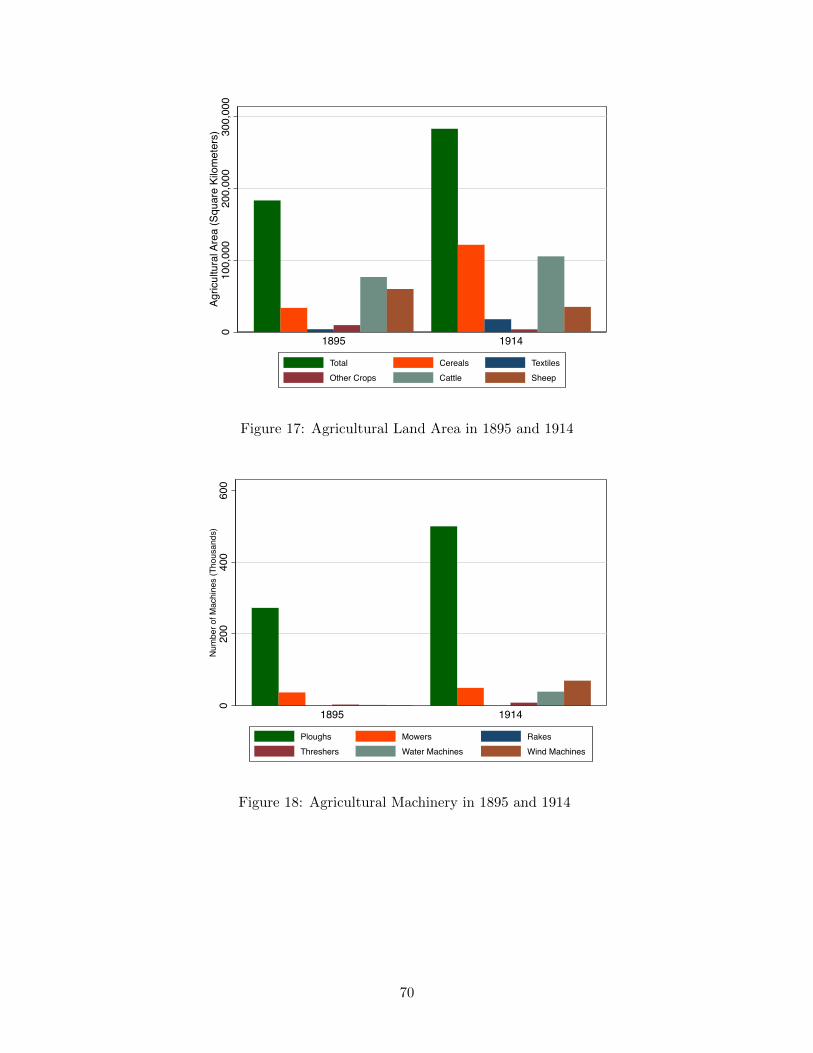
Figure 17 in this web appendix shows that these changes in export composition are reflected in

changes in relative agricultural land allocations, with a marked rise in Cereals agricultural area from

1895-1914. Table 2 of the paper reports the shares of agricultural machinery in imports. Figure 18

in this web appendix shows the total number of agricultural machines over time (ploughs, mowers,

rakes, threshers, water pumps and wind pumps), where the totals displayed in this figure are the

sum of the numbers reported for 1895 and 1914 for each district in our census data.

As shown in Section A.2 above, when transport costs di↵er across goods, the model predicts that

more remote locations export a narrower range of products. In Figure 19, we provide empirical

evidence on this prediction. We asign customs to the province in which they are located, and

display the number of exported products in 1869, 1895 and 1914 for each province, where provinces

are sorted by 1914 export values. Consistent with the model’s predictions, we find that more

geographically remote provinces not only have lower total export values but also on average export

a smaller number of products.

63

A.5 Data Appendix

A.5.1 District boundaries

The unit of analysis is the partido or departamento (which we refer to as “district” from now on).

These districts correspond to the first administrative division within a province (the name partido

is only used in the province of Buenos Aires, whilst in the other provinces the name departamento

prevails).

The actual administrative division used in this paper corresponds to the one reported in the

1895 population census, when there were 23 provinces or national territories and 386 districts. The

boundaries correspond to those drawn by Cacopardo (1967) with reference to that year. The same

publication includes maps corresponding to the administrative divisions in place in 1869 and 1914

and a concordance table which links the districts listed in every census between them. Both sets of

information – the maps and the table – were used to assign the data contained in the 1869 and 1914

census to constant spatial units based on the districts reported in the 1895 census. The process

of reassigning the data is discussed for each variable in turn in the remaining subsections of this

appendix.

A.5.2 Urban population

The 1869, 1895 and 1914 censuses all include figures for urban population at the district level.

In order to recreate the 1869 and 1914 urban populations of districts within 1895 boundaries the

following procedure was carried out:

- When a 1869 or 1914 district was entirely contained within a given 1895 district, the urban

population for 1869 and 1914 was entirely assigned to that 1895 district.

- When a 1869 or 1914 district was split among several 1895 districts, the location of the

main urban center at each year was established using secondary sources (Google Earth) and it was

determined to which 1895 district it belonged. All the urban population reported for the 1869 and

1914 districts was assigned to the 1895 district where the main urban center was located.

A.5.3 Rural population

The 1869, 1895 and 1914 census all include figures for rural population at the district level. In

order to recreate the 1869 and 1914 rural populations of districts within the 1895 boundaries the

following procedures were carried out:

- When a 1869 or 1914 district was entirely contained within a given 1895 district, the rural

population for 1869 and 1914 was entirely assigned to that 1895 district.

- When a 1914 district was split among several 1895 districts, an overlap of the 1895 admin-

istrative map with the 1914 administrative map was constructed using GIS software, and it was

determined which portion of the 1914 districts corresponded to the 1895 districts. Under the as-

sumption of a uniform density of the rural population within each 1914 district, the 1914 rural

64

population was assigned to the relevant 1895 districts.

- When a 1869 district was split among several 1895 districts, an equivalent method to the one

used for the 1914/1895 match was used. Since no 1869 district ceded territory to more than one

new 1895 district, it was possible to estimate the portions of each 1869 district that corresponded

to a given 1895 district simply by comparing the land extensions reported in 1869 and 1895. Under

the assumption of a uniform density of the rural population within each 1869 district, the 1869

rural population was assigned to the relevant 1895 districts.

A.5.4 Aggregate and Customs trade

The trade data was collected from di↵erent o�cial publications. For the data correspoding

to 1870, it was obtained from the statistical yearbook Estadısticas de las aduanas de la Republica

Argentina published by the Oficina de estadıstica general de la direccion de aduanas (the Statistical

O�ce of the Customs Direction). The data includes the quantity and value of the exports (by

destination) and imports (by origin) for each custom of the country following a relatively aggregated

product classification. For the data corresponding to 1895 and 1914, the same variables were

obtained from the statistical yearbook of the Direccion General de Estadıstica (Statistics General

Direction). The product classification is di↵erent to the one of 1870 and is more disaggregated.

A concordance between the di↵erent product classifications was constructed to make the data for

the three years comparable. Lastly, the geographical coordinates for each custom were determined

using Google Earth. The customs were then mapped into our spatial units of analysis, the districts

reported in the 1895 census, using GIS software.

A.5.5 Railways lines and stations

The location of the railway lines was established by digitizing the maps of the railway network

of Argentina for 1869, 1895 and 1914 included in Randle (1981). The list of stations operating in

each year was obtained from Estadısticas de los ferrocarriles en explotacion, a yearly publication of

the Direccion nacional de ferrocarriles (National Railways Direction) for 1895 and 1914 and from

historical sources for 1869. Two variables were collected for each railway station in the database:

its geographical coordinates and its opening date. The geographical coordinates of stations were

determined using Google Earth and Wikimapia taking into account changes in station names over

time. The stations were then mapped into our spatial units of analysis, the districts reported in the

1895 census, using GIS software. To determine the opening dates of stations, we used the opening

date of the section of the railway line on which the station is located. This information is available

in Estadısticas de los ferrocarriles en explotacion. Three dates for each section of a railway line

are available: the date when the construction was authorized, the date when the decree opening

the section was issued and the actual date when service was started (generally a few months after

the issuance of the decree). We used the last date whenever it was available. If this last date was

unavailable, the opening decree issuance date was used.

65

A.5.6 Railway shipments

The railway shipments data comes from Estadısticas de los ferrocarriles en explotacion. The

data is available on a yearly basis for all years starting in 1895. The records include the cargo

loaded in almost every station of the network. With respect to the records for the years 1895 and

1914 used in this paper, there is no data for Ferrocarril Central Cordoba (Central Cordoba Railway)

in 1895 and for the Ferrocarril Midland (Midland Railway) in 1914. The classification of products

di↵ers somewhat across railway lines. To construct a common product classification, we aggregated

similar categories (raw hides, bovine hides, sheep hides, etc.) into broader categories (hides) which

were common across railway lines.

A.5.7 Spanish Colonial Sixteenth Century Cities

Table 6 reports the Spanish colonial 16th-century cities used to construct our Route C16 in-

strument (Randle 1981).

66

References

[1] Cacopardo, Marıa Cristina (1967) Republica Argentina: Cambios en Los Limites Nacionales,

Provinciales y Departmentales, A Traves de Los Censos Nacionales de Poblacion, Buenos

Aires: Instituto Torcuato Di Tella.

[2] Direccion General de Estadıstica (1895) Anuario de la Direccion General de Estadıstica, Buenos

Aires.

[3] Direccion General de Estadıstica (1914) Anuario de la Direccion General de Estadıstica, Buenos

Aires.

[4] Direccion Nacional de Ferrocarriles (1895) Estadısticas de los Ferrocarriles en Explotacion,

Buenos Aires.

[5] Direccion Nacional de Ferrocarriles (1895) Estadısticas de los Ferrocarriles en Explotacion,

Buenos Aires.

[6] Oficina de Estadıstica General de la Direccion de Aduanas (1870) Estadısticas de las Aduanas

de la Republica Argentina, Buenos Aires.

[7] Randle, Patricio H. (1981) Atlas del Desarrollo Territorial de la Argentina, Buenos Aires:

Oikos.

67

Figure 13: Urban Population Shares 1869

Figure 14: Urban Population Shares 1895

68

Figure 15: Urban Population Shares 1914

Figure 16: Province Urban Population Share and Non-Agriculture Employment Shares 1914

69

010

0,00

020

0,00

030

0,00

0Ag

ricul

tura

l Are

a (S

quar

e Ki

lom

eter

s)

1895 1914

Total Cereals TextilesOther Crops Cattle Sheep

Figure 17: Agricultural Land Area in 1895 and 1914

020

040

060

0N

umbe

r of M

achi

nes

(Tho

usan

ds)

1895 1914

Ploughs Mowers RakesThreshers Water Machines Wind Machines

Figure 18: Agricultural Machinery in 1895 and 1914

70

050

100

150

Num

ber o

f exp

orte

d pr

oduc

ts

Buen

os A

ires

Sant

a Fe

Entre

Rio

s

Cor

doba

Cor

rient

es

Cha

co

Rio

Neg

ro

Chu

but

Sant

a C

ruz

Mis

ione

s

Form

osa

Salta

Juju

y

Men

doza

San

Juan

Cat

amar

ca

La R

ioja

Note: Number of products exported from customs in each province. Provinces sorted by 1914 export value

1870 1895 1914

Figure 19: Province Export Values and Number of Exported Products

71

Table A1: Sixteenth Century Cities

Province Name Year Founded

Buenos Aires Buenos Aires 1580 Buenos Aires Santa María del Buen Ayre 1536 Catamarca Londres 1558 Catamarca San Pedro de Mercado de Andalgalá 1582 Chaco Matará y Guacará 1585 Chaco Nuestra Señora de la Concepción del Bermejo 1585 Corrientes Vera en las 7 Corrientes 1588 Córdoba Alta Gracia 1590 Córdoba Córdoba 1573 Córdoba Santa María - Córdoba Santa Rosa de Calamuchita - Jujuy Humahuaca 1596 Jujuy Nieva 1561 Jujuy San Francisco de Alava 1575 Jujuy San Salvador de Jujuy 1593 La Rioja Todos Santos de La Nueva Rioja 1591 Mendoza Ciudad de la Resurección de Mendoza 1561 Mendoza Mendoza 1562 Salta Córdoba del Calchaquí 1551 Salta Esteco (Caceres) 1566 Salta Lerma en el Valle de Salta 1582 Salta Madrid de Las Juntas 1592 Salta Metán Viejo - Salta Nuestra Señora de Talavera 1567 Salta Primera San Clemente de la Nueva Sevilla 1577 Salta Segunda y Tercera San Clemente de la Nueva Sevilla 1577 Salta Segundo Barco 1559 San Juan San Juan de la Frontera 1562 San Luis San Luis de Loyola 1593 Santa Fe Corpus Christi 1536 Santa Fe Nuestra Señora de la Buena Esperanza 1536 Santa Fe Sancti Spiritus 1527 Santa Fe Santa Fe (Cayasta) 1573 Santiago del Estero Santiago del Nuevo Maestrazgo del Estero 1553 Santiago del Estero Tercer Barco 1552 Tucumán Amaicha - Tucumán Cañete 1560 Tucumán El Barco 1550 Tucumán Quilmes - Tucumán Ranchillos - Tucumán San Miguel de Tucumán 1565

Table 6: Spanish Colonial 16th-Century Cities

72