web effort estimation: function point analysis vs. cosmic · context: software development effort...
TRANSCRIPT
Information and Software Technology 72 (2016) 90–109
Contents lists available at ScienceDirect
Information and Software Technology
journal homepage: www.elsevier.com/locate/infsof
Web Effort Estimation: Function Point Analysis vs. COSMIC
Sergio Di Martino a, Filomena Ferrucci b,∗, Carmine Gravino b, Federica Sarro c
a Dipartimento di Ingegneria Elettrica e delle Tecnologie dell’Informazione, University of Napoli “Federico II”, Italyb Department of Computer Science, University of Salerno, Italyc CREST, Department of Computer Science, University College London, United Kingdom
a r t i c l e i n f o
Article history:
Received 7 July 2015
Revised 6 December 2015
Accepted 6 December 2015
Available online 23 December 2015
Keywords:
Web Effort Estimation
Functional Size Measures
COSMIC
IFPUG Function Point Analysis
a b s t r a c t
Context: software development effort estimation is a crucial management task that critically depends
on the adopted size measure. Several Functional Size Measurement (FSM) methods have been proposed.
COSMIC is considered a 2nd generation FSM method, to differentiate it from Function Point Analysis (FPA)
and its variants, considered as 1st generation ones. In the context of Web applications, few investigations
have been performed to compare the effectiveness of the two generations. Software companies could
benefit from this analysis to evaluate if it is worth to migrate from a 1st generation method to a 2nd
one.
Objective: the main goal of the paper is to empirically investigate if COSMIC is more effective than
FPA for Web effort estimation. Since software companies using FPA cannot build an estimation model
based on COSMIC as long as they do not have enough COSMIC data, the second goal of the paper is to
investigate if conversion equations can be exploited to support the migration from FPA to COSMIC.
Method: two empirical studies have been carried out by employing an industrial data set. The first
one compared the effort prediction accuracy obtained with Function Points (FPs) and COSMIC, using two
estimation techniques (Simple Linear Regression and Case-Based Reasoning). The second study assessed
the effectiveness of a two-step strategy that first exploits a conversion equation to transform historical
FPs data into COSMIC, and then builds a new prediction model based on those estimated COSMIC sizes.
Results: the first study revealed that, on our data set, COSMIC was significantly more accurate than FPs
in estimating the development effort. The second study revealed that the effectiveness of the analyzed
two-step process critically depends on the employed conversion equation.
Conclusion: for Web effort estimation COSMIC can be significantly more effective than FPA. Neverthe-
less, additional research must be conducted to identify suitable conversion equations so that the two-step
strategy can be effectively employed for a smooth migration from FPA to COSMIC.
© 2015 Elsevier B.V. All rights reserved.
F
i
M
m
F
f
s
n
F
e
a
c
f
1. Introduction
A crucial task for software project management is to accurately
estimate the effort required to develop an application, since this
estimate is usually a key factor for making a bid, planning the
development activities, allocating resources adequately, and so on.
Indeed, development effort, meant as the work carried out by soft-
ware practitioners, is the dominant project cost, being also the
most difficult to estimate and control. Significant over- or under-
estimates can be very expensive and deleterious for the competi-
tiveness of a software company [1].
FSM methods are meant to measure the software size by quan-
tifying the ”functionality” provided to the users. In particular, the
∗ Corresponding author. Tel.: +39 89963374.
E-mail addresses: [email protected] (S. Di Martino), [email protected] (F.
Ferrucci), [email protected] (C. Gravino), [email protected] (F. Sarro).
t
a
b
http://dx.doi.org/10.1016/j.infsof.2015.12.001
0950-5849/© 2015 Elsevier B.V. All rights reserved.
unction Point Analysis (FPA) was the first FSM method, defined
n 1979 [2]. Since then, several variants have been proposed (e.g.,
arkII and NESMA) with the aim of improving the size measure-
ent or extending the applicability domains [3]. As a consequence,
SM methods are nowadays widely applied in the industrial field
or sizing software systems and then using the obtained functional
ize as independent variable in estimation models. It is worth
oting that all the above methods fall in the 1st generation of
SM methods, distinguishing them from COSMIC, which is consid-
red a 2nd generation FSM method, due to several specific char-
cteristics. In particular, COSMIC was the first FSM approach con-
eived to comply to the standard ISO/IEC14143/1 [4]. It is based on
undamental principles of software engineering and measurement
heory, and it was developed to be suitable for a broader range of
pplication domains [5].
In the context of Web applications, few investigations have
een performed to analyze and assess the use of FPA (e.g., [6–8]).
S. Di Martino et al. / Information and Software Technology 72 (2016) 90–109 91
A
s
H
w
o
d
b
f
w
o
t
p
t
t
o
b
t
n
p
o
F
i
m
e
i
t
C
B
i
u
R
[
R
R
p
R
a
s
s
W
s
t
d
a
t
h
w
i
a
p
[
m
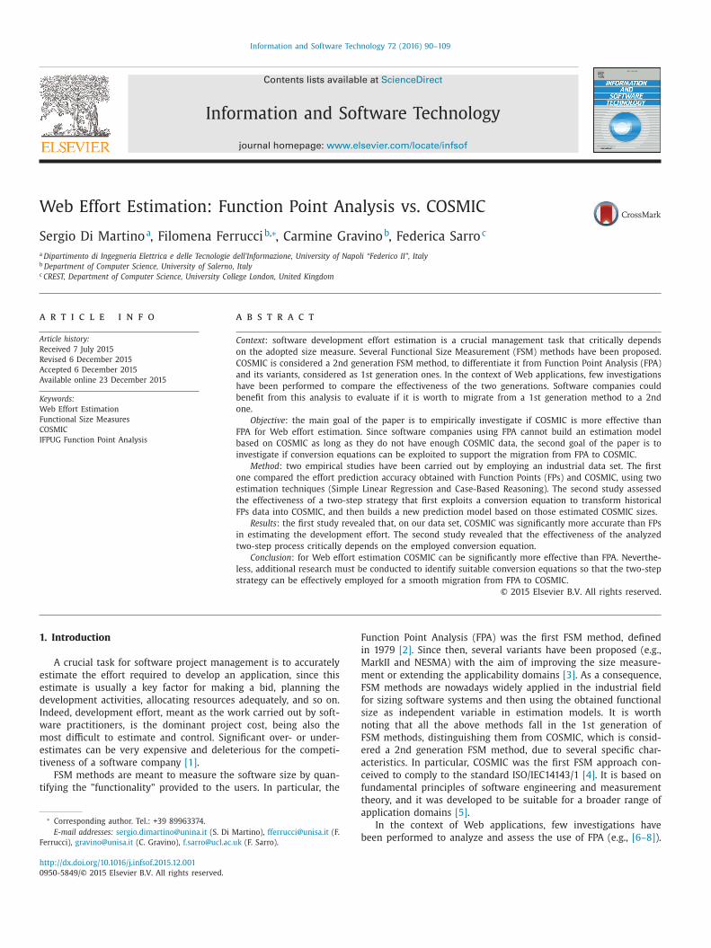
Fig. 1. The two-step process for building effort estimation models (2SEP).
n
t
p
p
a
p
s
g
t
t
C
p
e
s
s
r
F
f
c
t
p
a
a
M
t
b
f
w
s
t
c
p
[
f
e
few studies have also been carried out on the use of COSMIC for
izing Web applications and estimating development effort [9–13].
owever, no study compared the effectiveness of using COSMIC
ith respect to the use of FPA for Web effort estimation. More-
ver, only few studies were based on industrial experiences, also
ue to the lack of suitable data sets including information about
oth COSMIC and FPA sizes, and effort data. Thus, there is the need
or more empirical studies in this context that can support soft-
are companies in the choice of one of these measurement meth-
ds. A possible empirical evidence that COSMIC is more effective
han FPA for effort estimation could motivate those software com-
anies that usually employ FPA to migrate to COSMIC. It is evident
hat the migration from the 1st generation measurement methods
o the 2nd generation requires some additional costs. Indeed, not
nly it is necessary to acquire new expertise within the company,
ut there is also the need to compute again the size of the applica-
ions measured in the past with FPA, in order to use them to build
ew effort estimation models based on COSMIC [14,15] or for other
urposes (e.g., productivity benchmarking).
These issues motivated our investigation. Thus, the main aim
f this work is to assess whether COSMIC is more effective than
PA for the effort estimation of Web applications. To this end, we
nvestigated the following research question:
RQ1a Is the COSMIC measure significantly better than FPs for
estimating Web application development effort by using
Simple Linear Regression and Case Based Reasoning?
In the case we have indications that size in terms of COSMIC is
ore informative than the size in terms of FPs, it would be inter-
sting to highlight which characteristics contribute more in such
nformation [16]. Since for each application we have data about
he Base Functional Components (BFCs) that give cumulatively the
OSMIC size and FP sizes, we employed them to investigate which
FCs are more informative for predicting the effort. To this end, we
nvestigated the following research question:
RQ1b Which COSMIC and FP BFCs are significant in estimating
Web application development effort?
To answer RQ1a and RQ1b we performed an empirical study
sing data from 25 industrial Web applications. In particular, for
Q1a we employed two widely and successfully used techniques
17] for building effort estimation models, namely Simple Linear
egression (SLR), that is a model-based approach, and Case-Based
easoning (CBR), that is a Machine Learning-based solution, for
redicting the development effort.1 On the other hand, to answer
Q1b, we verified the correlation between each BFC and the effort
nd analyzed the distribution of the BFCs with respect to the final
ize.
A positive answer to the first research question might motivate
oftware companies to migrate from FPA to COSMIC for sizing new
eb applications, but also raises the question on how to manage
uch a transition. Indeed, a company would be interested in how
o start using COSMIC for effort estimation having only an internal
atabase of past project measured with FPA, thus without any suit-
ble estimation model for the new measure. The simplest strategy
o estimate the effort of new applications, until there is not enough
istorical data based on COSMIC, is to remeasure the past projects
ith this method, but this requires a lot of time and effort and
n some cases it cannot be possible due to the lack of appropri-
te information. Another solution could be to exploit a (linear or
1 Notice that we did not take into account other estimation methods, e.g., Sup-
ort Vector Regression [18], [19], Search-based approaches [20], and Web-COBRA
10], or combination of techniques, e.g., [21], since our focus was to compare FSM
ethods rather than specific techniques.
f
f
w
n
on-linear) conversion equation proposed in the literature to ob-
ain COSMIC sizes from the old FPs ones [14]. This allows the com-
any to exploit its historical FPs data using a two-step estimation
rocess (2SEP from here on) for building effort estimation models
s shown in Fig. 1. In more details, the first step consists of ap-
lying a conversion equation to each project in the historical data
et, to get an estimated COSMIC size starting from the FP one. This
ives to the software company a new historical data set based on
he estimated COSMIC. In the second step, it is possible to exploit
his data set and SLR (or another estimation technique) to build a
OSMIC based effort estimation model. This model can be used to
redict the effort of the new applications, now sized with COSMIC.
We are aware of the possibility that effort estimations based on
stimated sizes can be less accurate than the ones based on mea-
ured sizes. A company would be interested in using 2SEP for a
mooth migration if the obtained effort predictions have an accu-
acy at least not significantly worse than that obtained still using
PA. So, to analyze the effectiveness of 2SEP we investigated the
ollowing research question:
RQ2a Is the Web effort estimation accuracy obtained employing
2SEP, with (linear and non-linear) external conversion equa-
tions, not significantly worse than the accuracy achieved by
exploiting FPs in models built with SLR?
It is worth noting that another strategy for a software company
ould be to remeasure a sample of projects with COSMIC and use
hat subset to build an internal conversion equation that can be ex-
loited in the first step of 2SEP to get an estimated COSMIC size for
ll the other projects of the historical data set. Nevertheless, this
pproach requires the extra effort to remeasure in terms of COS-
IC at least a sample of projects. In the present paper we inves-
igated also the effectiveness of 2SEP using conversion equations
uilt on a sample of the 25 projects by analyzing how good was ef-
ort estimation using such company-specific equations. To this end,
e investigated the following research question:
RQ2b Is the Web effort estimation accuracy obtained employing
2SEP, with (linear and non-linear) internal conversion equa-
tions, not significantly worse than the accuracy achieved by
exploiting FPs in models built with SLR?
To answer RQ2a and RQ2b we performed a second empirical
tudy employing the same data set of 25 Web applications used in
he first one, some external conversion equations and the internal
onversion equations built considering a small sample of Web ap-
lications. To the best of our knowledge, the previous studies (e.g.,
14,22,23]) investigating the conversion from FPs to COSMIC sizes
ocused only on showing that it is possible to build conversion
quations, while the present study is the first that assesses the ef-
ectiveness of the sizes obtained using some conversion equations
or effort estimation purposes.
The remainder of the paper is organized as follows. In Section 2
e briefly describe the FSM methods employed in our study,
amely FPA and COSMIC, and then we present related work on the
92 S. Di Martino et al. / Information and Software Technology 72 (2016) 90–109
I
o
p
2
s
s
t
fi
d
B
r
b
a
o
c
p
a
c
r
2
t
h
t
s
p
use of FPA and COSMIC for Web effort estimation. In Sections 3
and 4 we present the two performed empirical studies. Threats to
validity of both empirical studies are discussed in Section 5, while
Section 6 concludes the paper giving some final remarks.
2. Background
In the following, we provide a brief history of FSM methods and
recall the main notions of FPA and COSMIC.
2.1. A brief history of FSM methods
Software size measures can be grouped in two main families:
the Functional and Dimensional ones. A Functional Size Measure is
defined as “a size of software derived by quantifying the Functional
User Requirements (FURs)” [4]. Thus, FSMs are particularly suit-
able to be applied in the early phases of the development lifecycle,
when only FURs are available, being the typical choice for tasks
such as estimating a project development effort. Moreover, they
are independent from the adopted technologies, allowing compar-
isons among projects developed with different platforms, solutions,
and so on. Dimensional sizes basically count some structural prop-
erties of a software artifact, such as LOCs, number of Web pages,
and so on. They can be applied only after the artifact has been
developed, they are strongly dependent on the adopted technolog-
ical solutions, and often a standard counting procedure is missing
[24,25]. The first FSM method proposed in the literature was the
FPA, introduced by Albrecht in 1979 [2] as a measure (the Func-
tion Points) to overcome the limitations of LOCs, by quantifying the
”functionality” provided by a software, from the end-user point of
view. Indeed, FPA can be seen as a structured method to perform a
functional decomposition of the system. In this way, its size can be
considered as the (weighted) sum of unitary elements (its FURs),
that can be measured more easily than the whole system. FPA has
evolved in many different ways. The original formulation was ex-
tended by Albrecht and Gaffney [26]. Then, since 1986 FPA is man-
aged by the International Function Point Users Group (IFPUG) [27]
and it is named IFPUG FPA (IFPUG, for short), which has been stan-
dardized by ISO as ISO/IEC 20926:2009. Nevertheless, since FPA
was designed from the experience gained by Albrecht on the de-
velopment of Management Information Systems, the applicability
of this method to other software domains has been highly debated
(e.g., [28,29]). As a consequence, many variants of FPA were de-
fined for specific domains, such as MkII Function Point for data-
rich business applications, or Full Function Point (FFP) method for
embedded and control systems [3]. Since these methods are all
based on the original formulation by Albrecht, they are also known
as 1st generation FSM methods.
In the middle of the 90s, some researchers highlighted impor-
tant issues in the foundations of FPA against the measurement the-
ory. Indeed, in many steps of the FPA process an improper use
of different types of scales was highlighted. Moreover, how the
”weights” were defined and used in the method has been object
of discussion in the literature (e.g., [30,31]).
To overcome these issues, and also to define a broader mea-
surement framework able to tackle new IT challenges, at the end
of the 90s a group of experienced software measurers formed the
Common Software Measurement International Consortium (COS-
MIC), whose result was the COSMIC-FFP method, which is consid-
ered the first “2nd generation FSM method”. To highlight this con-
cept, the first version of the method was the 2.0. Many important
refinements were introduced in 2007 in the version 3.0, named
simply COSMIC, and standardized as ISO/IEC 19761:2011. The cur-
rent version of COSMIC is 4.0.1, introduced in April 2015.
In the following we describe the main concepts underlying the
FPUG and the COSMIC methods. Among the 1st generation meth-
ds, we analyze IFPUG since it is the most widely used by software
ractitioners.
.2. The IFPUG method
IFPUG sizes an application starting from its FURs (or by other
oftware artifacts that can be abstracted in terms of FURs).
In particular, to identify the set of “features” provided by the
oftware, each FUR is functionally decomposed into Base Func-
ional Components (BFC), and each BFC is categorized into one of
ve Data or Transactional BFC Types. The Data functions can be
efined as follows:
• Internal Logical Files (ILF) are logical, persistent entities main-
tained by the application to store information of interest.
• External Interface Files (EIF) are logical, persistent entities that
are referenced by the application, but are maintained by an-
other software application.
The Transactional ones are defined as follows:
• External Inputs (EI) are logical, elementary business processes
that cross into the application boundary to maintain the data
on an Internal Logical File.
• External Outputs (EO) are logical, elementary business pro-
cesses that result in data leaving the application boundary to
meet a user requirements (e.g., reports, screens).
• External Inquires (EQ) are logical, elementary business pro-
cesses that consist of a data trigger followed by a retrieval
of data that leaves the application boundary (e.g., browsing of
data).
Once the BFCs have been identified, the “complexity” of each
FC is assessed. This step depends on the kind of function type and
equires the identification of further attributes (such as the num-
er of data fields to be processed). Once derived this information,
table provided in the IFPUG method [27] specifies the complexity
f each function, in terms of Unadjusted Function Points (UFP).
The sum of all these UFPs gives the functional size of the appli-
ation. Subsequently, a Value Adjustment Factor (VAF) can be com-
uted to take into account some non-functional requirements, such
s Performances, Reusability, and so on. The final size of the appli-
ation in terms of Function Points is given by FP = UFP · VAF .
For more details about the application of the IFPUG method,
eaders may refer to the counting manual [27].
.3. The COSMIC method
The basic idea underlying the COSMIC method is that, for many
ypes of software, most of the development efforts are devoted to
andle data movements from/to persistent storage and users. Thus,
he number of these data movements can provide a meaningful
ight of the system size [5]. As a consequence, the measurement
rocess consists of three phases:
1. The Measurement Strategy phase is meant to define the purpose
of the measurement, the scope (i.e. the set of FURs to be in-
cluded in the measurement), the functional users of each piece
of software (i.e. the senders and intended recipients of data
to/from the software to be measured), and the level of granu-
larity of the available artifacts.
2. The Mapping Phase is a crucial process to express each FUR in
the form required by the COSMIC Generic Software Model. This
model, necessary to identify the key elements of a FUR to be
measured , assumes that (I) each FUR can be mapped into a
unique functional process, meant as a cohesive and indepen-
dently executable set of data movements, (II) each functional
S. Di Martino et al. / Information and Software Technology 72 (2016) 90–109 93
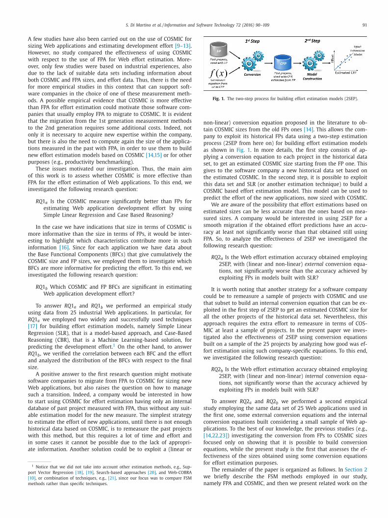
Fig. 2. The four types of data movements, and their relationship with a functional
process [5].
t
2
m
v
t
M
o
h
f
e
t
i
a
t
f
a
e
v
b
(
2
t
a
i
i
[
b
fi
i
[
p
t
s
r
W
i
T
i
c
t
c
m
e
t
e
w
O
W
u
p
i
c
t
p
h
o
e
c
c
t
t
R
b
p
m
s
d
l
F
[
e
w
F
t
p
b
r
a
process consists of sub-processes, and (III) each sub-process
may be either a data movement or a data manipulation. To
measure these data movements, three other concepts have to
be identified. A Triggering Event is an action of a functional user
of the piece of software triggering one or more functional pro-
cesses. A Data Group is a distinct, non-empty and non-ordered
set of data attributes, where each attribute describes a comple-
mentary aspect of the same object of interest. A Data Attribute
is the smallest piece of information, within an identified data
group, carrying a meaning from the perspective of the inter-
ested FUR. As depicted in Fig. 2, data movements are defined
as follows:
• An Entry (E) moves a data group from a functional user
across the boundary into the functional process where it is
required.
• An Exit (X) moves a data group from a functional process
across the boundary to the functional user that requires it.
• A Read (R) moves a data group from persistent storage
within each of the functional process that requires it.
• A Write (W) moves a data group lying inside a functional
process to persistent storage.
3. The Measurement Phase, where the data movements of each
functional process have to be identified and counted. Each of
them is counted as 1 COSMIC Function Point (CFP) that is the
COSMIC measurement unit. Thus, the size of an application
within a defined scope is obtained by summing the sizes of all
the functional processes within the scope.
For more details about the COSMIC method, readers are referred
o the COSMIC Measurement Manual [5].
.4. Related work
In the literature there is a number of studies on the assess-
ent of FPA and COSMIC methods for effort estimation. However,
ery few of them investigate their effectiveness for Web applica-
ions. It is worth to mention that besides Function Points and COS-
IC, other size measures (e.g., dimensional measures like number
f Web pages, media elements, client and server side scripts, etc.)
ave been proposed in the literature to be employed specifically
or Web application development effort in combination with sev-
ral estimation techniques [32–37]. However, since our focus is on
he use of FPA and COSMIC measurement methods, in the follow-
ng we first report on investigations exploiting FPA (Section 2.4.1)
nd then those employing COSMIC (Section 2.4.2), also considering
heir extensions/adaptions.
We will discuss the main studies proposing conversion models
rom FPs into COSMIC in Section 4.1. It is worth noting that the
nalysis about the effectiveness of internal vs. external conversion
quations is related to the studies investigating the use of cross-
s. within-company data sets for effort estimation. This topic has
een widely analyzed in the last years producing different results
see e.g., [38,39]).
.4.1. Using FPA and its extensions for Web effort estimation
FPA was employed by Ruhe et al. [40] to size 12 Web applica-
ions, such as B2B, intranet or financial, developed between 1998
nd 2002. The aim was to compare the effort estimations obtained
n terms of FPA with those achieved exploiting a size measure
ntroduced specifically for Web applications, namely Web Objects
41]. Web Objects method represents an extension of FPA provided
y Reifer who added four new Web-related components to the
ve function types of FPA, namely Multimedia Files, Web Build-
ng Blocks, Scripts, and Links. The results reported by Ruhe et al.
40] showed that the Web Objects-based linear regression model
rovided more accurate estimates than those achieved using Func-
ion Points. Successively, Web Objects measure was also used as
ize metric in the context of Web-COBRA [42], obtaining better
esults than those achieved with linear regression. Observe that
eb-COBRA is a composite estimation method obtained by adapt-
ng COBRA [43] to be applied in the context of Web applications.
he use of Web Objects for effort estimation was also exploited
n other studies [11,44]. In the first study [11], Web Objects were
ompared against COSMIC, by considering linear regression as es-
imation method, and the analysis of a data set of 15 Web appli-
ations revealed that the estimates achieved with a COSMIC based
odel were better. The second study [44] can be considered an
xtension of the previous one [11], by employing further applica-
ions in the data set, a further estimation technique (i.e., CBR), and
xploring a different validation method. In that study, Web Objects
ere also compared against FPs. The results confirmed that Web
bjects provided better results than FPs.
Other works proposed adaptations/extensions of FPA to size
eb applications and estimate the development effort. In partic-
lar, the OOmFPWeb method [7] maps the FPs concepts into the
rimitives used in the conceptual modeling phase of OOWS, which
s a method for producing software for the Web [45]. More re-
ently, Abrahão et al. have also proposed a model-driven func-
ional size measurement procedure, named OO-HFP, for Web ap-
lications developed using the OO-H method [46]. The approach
as been validated by comparing its estimation accuracy with the
ne achieved by using the set of measures defined by Mendes
t al. for the Tukutuku database [32]. The results of the empiri-
al study were promising since the obtained effort estimates were
omparable with those obtained by using the Tukutuku measures,
hus revealing that the OO-HFP approach can be suitable to es-
imate the development effort of model-driven Web applications.
ecently, the accuracy of the estimates achieved with OO-HFP has
een compared with the accuracy of estimates obtained by em-
loying a set of design measures defined on OO-H conceptual
odels [47]. By employing 30 OO-H Web applications the analy-
is revealed that the linear regression model based on two OO-H
esign measures provided significantly better estimates than the
inear model based on the OO-HFP measure, thus confirming that
PA can fail to capture some specific features of Web applications
6,48].
Another FPA based approach able to automatically obtain a size
stimation of Web applications from conceptual models produced
ith a model-driven development method has been provided by
raternali et al. [8]. In particular, the software models were ob-
ained by using WebML, a UML profile proposed to model Web ap-
lications [49]. An initial validation of the approach was performed
y comparing the FPs counting computed automatically with the
esult achieved by two skilled analysts who manually sized the
pplications. The analysis revealed that the average error between
94 S. Di Martino et al. / Information and Software Technology 72 (2016) 90–109
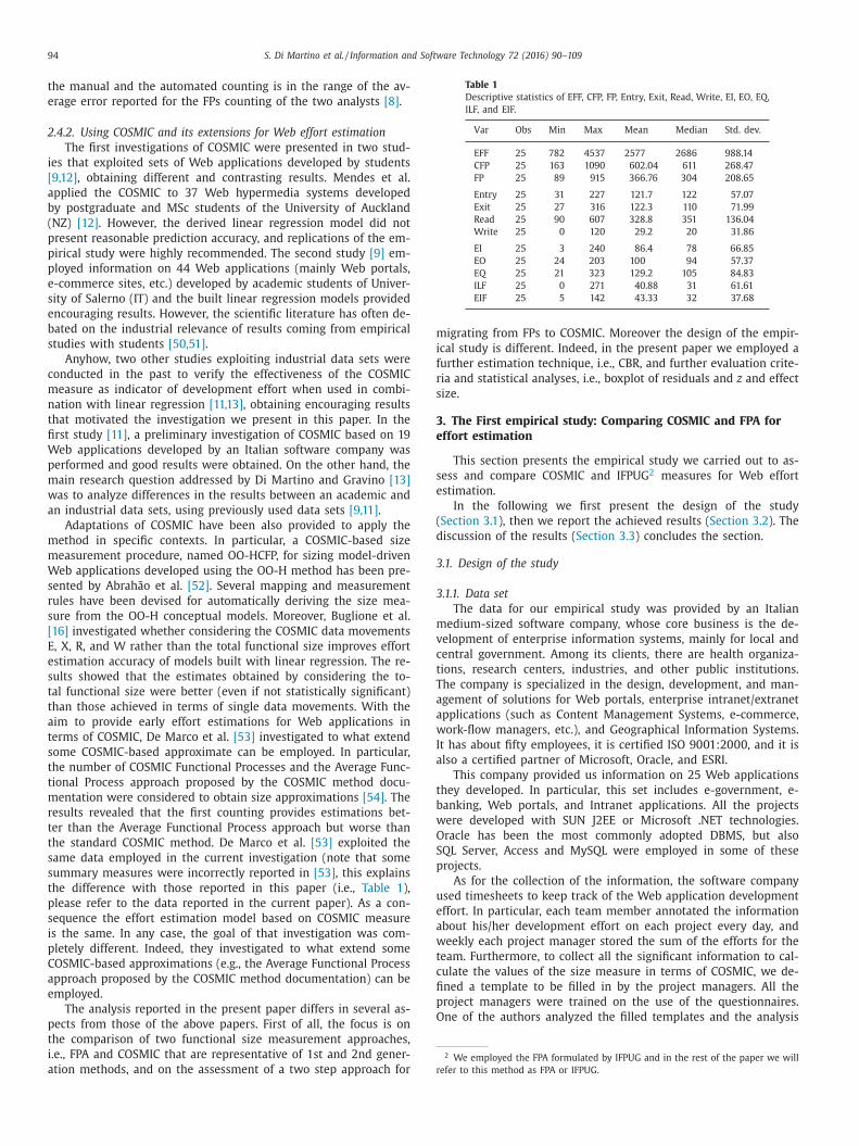
Table 1
Descriptive statistics of EFF, CFP, FP, Entry, Exit, Read, Write, EI, EO, EQ,
ILF, and EIF.
Var Obs Min Max Mean Median Std. dev.
EFF 25 782 4537 2577 2686 988.14
CFP 25 163 1090 602.04 611 268.47
FP 25 89 915 366.76 304 208.65
Entry 25 31 227 121.7 122 57.07
Exit 25 27 316 122.3 110 71.99
Read 25 90 607 328.8 351 136.04
Write 25 0 120 29.2 20 31.86
EI 25 3 240 86.4 78 66.85
EO 25 24 203 100 94 57.37
EQ 25 21 323 129.2 105 84.83
ILF 25 0 271 40.88 31 61.61
EIF 25 5 142 43.33 32 37.68
m
i
f
r
s
3
e
s
e
(
d
3
3
m
v
c
t
T
a
a
w
I
a
t
b
w
O
S
p
u
e
a
w
t
c
fi
p
O
2 We employed the FPA formulated by IFPUG and in the rest of the paper we will
refer to this method as FPA or IFPUG.
the manual and the automated counting is in the range of the av-
erage error reported for the FPs counting of the two analysts [8].
2.4.2. Using COSMIC and its extensions for Web effort estimation
The first investigations of COSMIC were presented in two stud-
ies that exploited sets of Web applications developed by students
[9,12], obtaining different and contrasting results. Mendes et al.
applied the COSMIC to 37 Web hypermedia systems developed
by postgraduate and MSc students of the University of Auckland
(NZ) [12]. However, the derived linear regression model did not
present reasonable prediction accuracy, and replications of the em-
pirical study were highly recommended. The second study [9] em-
ployed information on 44 Web applications (mainly Web portals,
e-commerce sites, etc.) developed by academic students of Univer-
sity of Salerno (IT) and the built linear regression models provided
encouraging results. However, the scientific literature has often de-
bated on the industrial relevance of results coming from empirical
studies with students [50,51].
Anyhow, two other studies exploiting industrial data sets were
conducted in the past to verify the effectiveness of the COSMIC
measure as indicator of development effort when used in combi-
nation with linear regression [11,13], obtaining encouraging results
that motivated the investigation we present in this paper. In the
first study [11], a preliminary investigation of COSMIC based on 19
Web applications developed by an Italian software company was
performed and good results were obtained. On the other hand, the
main research question addressed by Di Martino and Gravino [13]
was to analyze differences in the results between an academic and
an industrial data sets, using previously used data sets [9,11].
Adaptations of COSMIC have been also provided to apply the
method in specific contexts. In particular, a COSMIC-based size
measurement procedure, named OO-HCFP, for sizing model-driven
Web applications developed using the OO-H method has been pre-
sented by Abrahão et al. [52]. Several mapping and measurement
rules have been devised for automatically deriving the size mea-
sure from the OO-H conceptual models. Moreover, Buglione et al.
[16] investigated whether considering the COSMIC data movements
E, X, R, and W rather than the total functional size improves effort
estimation accuracy of models built with linear regression. The re-
sults showed that the estimates obtained by considering the to-
tal functional size were better (even if not statistically significant)
than those achieved in terms of single data movements. With the
aim to provide early effort estimations for Web applications in
terms of COSMIC, De Marco et al. [53] investigated to what extend
some COSMIC-based approximate can be employed. In particular,
the number of COSMIC Functional Processes and the Average Func-
tional Process approach proposed by the COSMIC method docu-
mentation were considered to obtain size approximations [54]. The
results revealed that the first counting provides estimations bet-
ter than the Average Functional Process approach but worse than
the standard COSMIC method. De Marco et al. [53] exploited the
same data employed in the current investigation (note that some
summary measures were incorrectly reported in [53], this explains
the difference with those reported in this paper (i.e., Table 1),
please refer to the data reported in the current paper). As a con-
sequence the effort estimation model based on COSMIC measure
is the same. In any case, the goal of that investigation was com-
pletely different. Indeed, they investigated to what extend some
COSMIC-based approximations (e.g., the Average Functional Process
approach proposed by the COSMIC method documentation) can be
employed.
The analysis reported in the present paper differs in several as-
pects from those of the above papers. First of all, the focus is on
the comparison of two functional size measurement approaches,
i.e., FPA and COSMIC that are representative of 1st and 2nd gener-
ation methods, and on the assessment of a two step approach for
igrating from FPs to COSMIC. Moreover the design of the empir-
cal study is different. Indeed, in the present paper we employed a
urther estimation technique, i.e., CBR, and further evaluation crite-
ia and statistical analyses, i.e., boxplot of residuals and z and effect
ize.
. The First empirical study: Comparing COSMIC and FPA for
ffort estimation
This section presents the empirical study we carried out to as-
ess and compare COSMIC and IFPUG2 measures for Web effort
stimation.
In the following we first present the design of the study
Section 3.1), then we report the achieved results (Section 3.2). The
iscussion of the results (Section 3.3) concludes the section.
.1. Design of the study
.1.1. Data set
The data for our empirical study was provided by an Italian
edium-sized software company, whose core business is the de-
elopment of enterprise information systems, mainly for local and
entral government. Among its clients, there are health organiza-
ions, research centers, industries, and other public institutions.
he company is specialized in the design, development, and man-
gement of solutions for Web portals, enterprise intranet/extranet
pplications (such as Content Management Systems, e-commerce,
ork-flow managers, etc.), and Geographical Information Systems.
t has about fifty employees, it is certified ISO 9001:2000, and it is
lso a certified partner of Microsoft, Oracle, and ESRI.
This company provided us information on 25 Web applications
hey developed. In particular, this set includes e-government, e-
anking, Web portals, and Intranet applications. All the projects
ere developed with SUN J2EE or Microsoft .NET technologies.
racle has been the most commonly adopted DBMS, but also
QL Server, Access and MySQL were employed in some of these
rojects.
As for the collection of the information, the software company
sed timesheets to keep track of the Web application development
ffort. In particular, each team member annotated the information
bout his/her development effort on each project every day, and
eekly each project manager stored the sum of the efforts for the
eam. Furthermore, to collect all the significant information to cal-
ulate the values of the size measure in terms of COSMIC, we de-
ned a template to be filled in by the project managers. All the
roject managers were trained on the use of the questionnaires.
ne of the authors analyzed the filled templates and the analysis
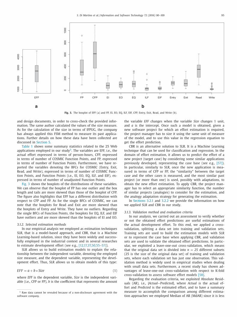
S. Di Martino et al. / Information and Software Technology 72 (2016) 90–109 95
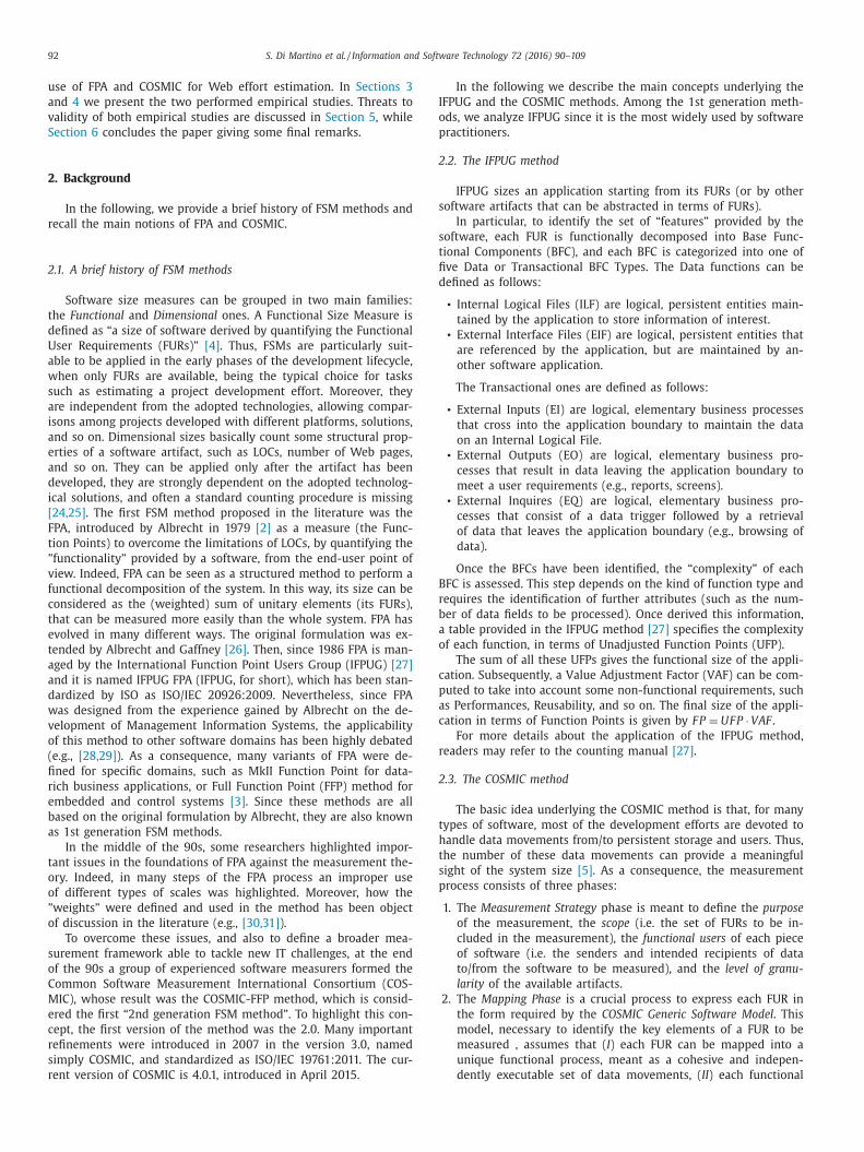
Fig. 3. The boxplot of EFF (a) and FP, EI, EO, EQ, ILF, EIF, CFP, Entry, Exit, Read, and Write (b).
a
m
A
h
t
d
a
a
i
i
p
R
t
p
W
l
T
r
n
t
t
h
3
S
L
f
t
t
s
o
E
w
a
s
t
a
n
t
o
g
t
d
n
p
I
s
c
p
o
a
o
t
w
3
o
t
v
T
o
s
u
t
(
s
i
w
v
c
nd design documents, in order to cross-check the provided infor-
ation. The same author calculated the values of the size measure.
s for the calculation of the size in terms of IFPUG, the company
as always applied this FSM method to measure its past applica-
ions. Further details on how these data have been collected are
iscussed in Section 5.
Table 1 shows some summary statistics related to the 25 Web
pplications employed in our study3. The variables are EFF, i.e., the
ctual effort expressed in terms of person-hours, CFP, expressed
n terms of number of COSMIC Function Points, and FP, expressed
n terms of number of Function Points. Furthermore, we have re-
orted the variables denoting the BFCs for COSMIC (Entry, Exit,
ead, and Write), expressed in terms of number of COSMIC Func-
ion Points, and Function Points (i.e., EI, EO, EQ, ILF, and EIF), ex-
ressed in terms of number of unadjusted Function Points.
Fig. 3 shows the boxplots of the distributions of these variables.
e can observe that the boxplot of FP has one outlier and the box
ength and tails are more skewed than those of the boxplot of CFP.
he figure also highlights that EFF has a different distribution with
espect to CFP and FP. As for the single BFCs of COSMIC, we can
ote that the boxplots for Read and Exit are more skewed than
he boxplots of Entry and Write. They have no outliers. Regarding
he single BFCs of Function Points, the boxplots for EQ, ILF, and EIF
ave outliers and are more skewed than the boxplots of EI and EO.
.1.2. Selected estimation methods
In our empirical analysis we employed as estimation techniques
LR, that is a model-based approach, and CBR, that is a Machine
earning-based solution, since they have been widely and success-
ully employed in the industrial context and in several researches
o estimate development effort (see e.g., [12,17,37,50,55–57]).
SLR allows us to build estimation models to explain the rela-
ionship between the independent variable, denoting the employed
ize measure, and the dependent variable, representing the devel-
pment effort. Thus, SLR allows us to obtain models of this type:
FF = a + b ∗ Size (1)
here EFF is the dependent variable, Size is the independent vari-
ble (i.e., CFP or FP), b is the coefficient that represents the amount
3 Raw data cannot be revealed because of a non-disclosure agreement with the
oftware company.
u
f
m
t
he variable EFF changes when the variable Size changes 1 unit,
nd a is the intercept. Once such a model is obtained, given a
ew software project for which an effort estimation is required,
he project manager has to size it using the same unit of measure
f the model, and to use this value in the regression equation to
et the effort prediction.
CBR is an alternative solution to SLR. It is a Machine Learning
echnique that can be used for classification and regression. In the
omain of effort estimation, it allows us to predict the effort of a
ew project (target case) by considering some similar applications
reviously developed, representing the case base (see e.g., [57]).
n particular, similarly to SLR, once the new application is mea-
ured in terms of CFP or FP, the “similarity” between the target
ase and the other cases is measured, and the most similar past
roject (or more than one) is used, possibly with adaptations, to
btain the new effort estimation. To apply CBR, the project man-
ger has to select an appropriate similarity function, the number
f similar projects (analogies) to consider for the estimation, and
he analogy adaptation strategy for generating the estimation.
In Sections 3.2.1 and 3.2.2 we provide the information on how
e applied SLR and CBR in our study.
.1.3. Validation method and evaluation criteria
In our analysis, we carried out an assessment to verify whether
r not the obtained effort predictions are useful estimations of
he actual development effort. To this end, we applied a cross-
alidation, splitting a data set into training and validation sets.
raining sets are used to build the estimation models with SLR
r to represent the case base when applying CBR, and validation
ets are used to validate the obtained effort predictions. In partic-
lar, we exploited a leave-one-out cross-validation, which means
hat the original data set is divided into n = 25 different subsets
25 is the size of the original data set) of training and validation
ets, where each validation set has just one observation. This val-
dation method is widely used in empirical studies when dealing
ith small data sets. Furthermore, a recent study has shown ad-
antages of leave-one-out cross-validation with respect to K-fold
ross-validation to assess software effort models [58].
Regarding the evaluation criteria, we exploited Absolute Resid-
als (AR), i.e., |Actual−Predicted|, where Actual is the actual ef-
ort and Predicted is the estimated effort, and to have a summary
easure to accomplish the comparison among different estima-
ion approaches we employed Median of AR (MdAR) since it is less
96 S. Di Martino et al. / Information and Software Technology 72 (2016) 90–109
200 400 600 800 1000
10
00
20
00
30
00
40
00
CFP
EF
F
1
2
3
4
5
67
8
9
10
1112
13
14
15
16
17
18
19
20
21
22
23
24
25
a
200 400 600 800
10
00
20
00
30
00
40
00
FP
EF
F
1
2
3
4
5
67
8
9
10
1112
13
14
15
16
17
18
19
20
21
22
23
24
25
b
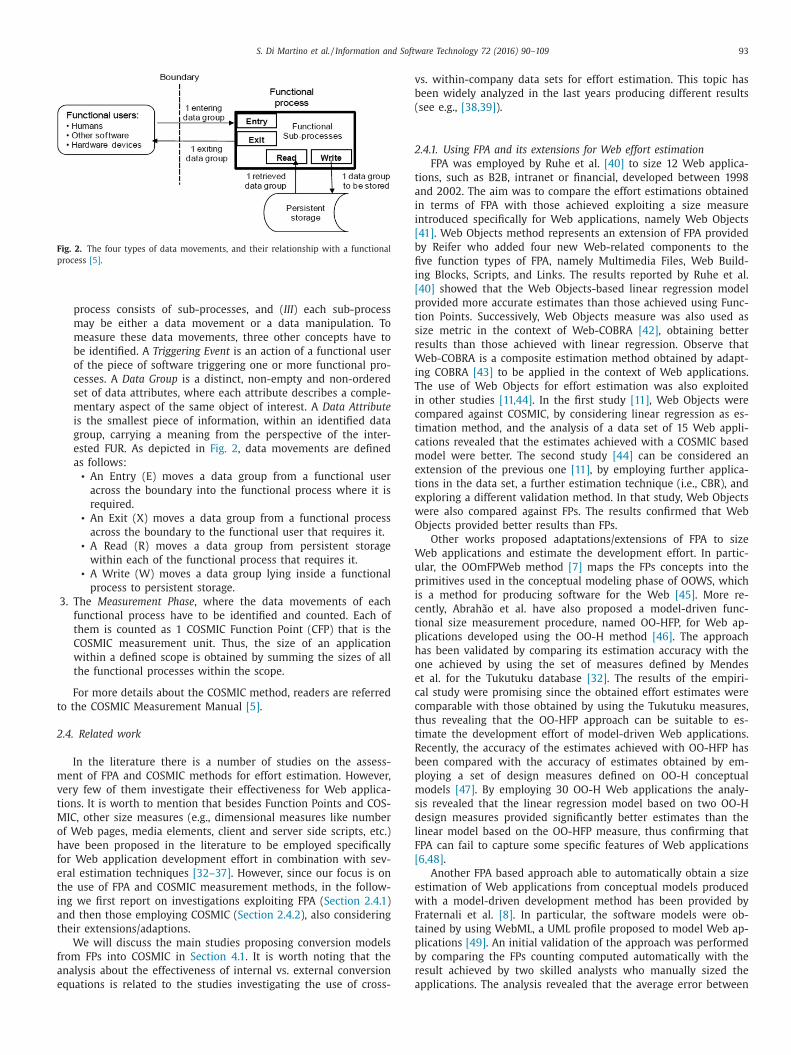
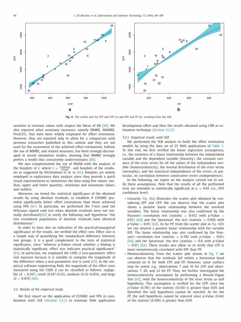
Fig. 4. The scatter plot for EFF and CFP (a) and EFF and FP (b), resulting from the SLR.
d
t
3
m
T
i
v
a
a
(
t
i
t
c
sensitive to extreme values with respect the Mean of AR [59]. We
also reported other summary measures, namely MMRE, MdMRE,
Pred(25), that have been widely employed for effort estimation.
However, they are reported only to allow for a comparison with
previous researches published in this context and they are not
used for the assessment of the achieved effort estimations. Indeed,
the use of MMRE, and related measures, has been strongly discour-
aged in recent simulation studies, showing that MMRE wrongly
prefers a model that consistently underestimates [60].
We also complemented the use of MdAR with the analysis of
the boxplots of z, where z = PredictedActual
, and boxplots of the residu-
als as suggested by Kitchenham et al. in [61]. Boxplots are widely
employed in exploratory data analysis since they provide a quick
visual representation to summarize the data using five values: me-
dian, upper and lower quartiles, minimum and maximum values,
and outliers.
Moreover, we tested the statistical significance of the obtained
results by using absolute residuals, to establish if COSMIC pro-
vided significantly better effort estimations than those achieved
using FPA [61]. In particular, we performed the T-test (and the
Wilcoxon signed rank test when absolute residuals were not nor-
mally distributed)[62] to verify the following null hypothesis “the
two considered populations of absolute residuals have identical
distributions”.
In order to have also an indication of the practical/managerial
significance of the results, we verified the effect size. Effect size is
a simple way of quantifying the standardized difference between
two groups. It is a good complement to the tests of statistical
significance, since “whereas p-Values reveal whether a finding is
statistically significant, effect size indicates practical significance”
[63]. In particular, we employed the Cliffs d non-parametric effect
size measure because it is suitable to compute the magnitude of
the difference when a non-parametric test is used [63]. In the em-
pirical software engineering field, the magnitude of the effect sizes
measured using the Cliffs d can be classified as follows: negligi-
ble (d < 0.147), small (0.147–0.33), medium (0.33–0.474), and large
(d > 0.474) [63].
3.2. Results of the empirical study
We first report on the application of COSMIC and FPA in com-
bination with SLR (Section 3.2.1) to estimate Web application
evelopment effort and then the results obtained using CBR as es-
imation technique (Section 3.2.2).
.2.1. Empirical results with SLR
We performed the SLR analysis to build the effort estimation
odels by using the data set of 25 Web applications of Table 1.
o this end, we first verified the linear regression assumptions,
.e., the existence of a linear relationship between the independent
ariable and the dependent variable (linearity), the constant vari-
nce of the error terms for all the values of the independent vari-
ble (homoscedasticity), the normal distribution of the error terms
normality), and the statistical independence of the errors, in par-
icular, no correlation between consecutive errors (independence).
In the following, we report on the analysis carried out to ver-
fy these assumptions. Note that the results of all the performed
ests are intended as statistically significant at α = 0.05 (i.e., 95%
onfidence level).
• Linearity. Fig. 4(a) illustrates the scatter plot obtained by con-
sidering EFF and CFP. We can observe that the scatter plot
shows a positive linear relationship between the involved
variables. The linear relationship was also confirmed by the
Pearson’s correlation test (statistic = 0.932 with p-Value <
0.01) [64] and the Spearman’ rho test (statistic = 0.942 with
p-Value < 0.01) [62]. As for FP, from the scatter plot in Fig. 4(b)
we can observe a positive linear relationship with the variable
EFF. The linear relationship was also confirmed by the Pear-
son’s correlation test (statistic = 0.782 with p-Value < 0.01)
[64] and the Spearman’ rho test (statistic = 0.8 with p-Value
< 0.01) [62]. These results also allow us to verify that CFP is
more monotonously correlated with EFF than FP.
• Homoscedasticity. From the scatter plot shown in Fig. 5 we
can observe that the residuals fall within a horizontal band
centered on 0, for both CFP and FP. However, some outliers
may be noted, e.g., observations 7 and 16 for CFP and obser-
vations 7, 20, and 22 for FP. Thus, we further investigated the
homoscedasticity assumption by performing a Breush–Pagan
Test [65], with the homoscedasticity of the error terms as null
hypothesis. This assumption is verified for the CFP, since the
p-Value (0.741) of the statistic (0.110) is greater than 0.05 and
therefore the null hypothesis cannot be rejected. As for the
FP, the null hypothesis cannot be rejected since p-Value (0.44)
of the statistic (0.596) is greater than 0.05.
S. Di Martino et al. / Information and Software Technology 72 (2016) 90–109 97
1000 1500 2000 2500 3000 3500 4000
-50
00
50
01
00
0
Fitted values with CFP
Re
sid
ua
ls
1 2
3
4
5
6
7
8
9
10
11
12
13
14
15
16
17
18
19
20
21
2223
24
25
a
1500 2000 2500 3000 3500 4000 4500
-10
00
-50
00
50
01
00
0
Fitted values with FP
Re
sid
ua
ls
1
2
3 45
6
7
8
9
10
11
12
13
14
1516
17 1819
20
21
22
23
24
25
b
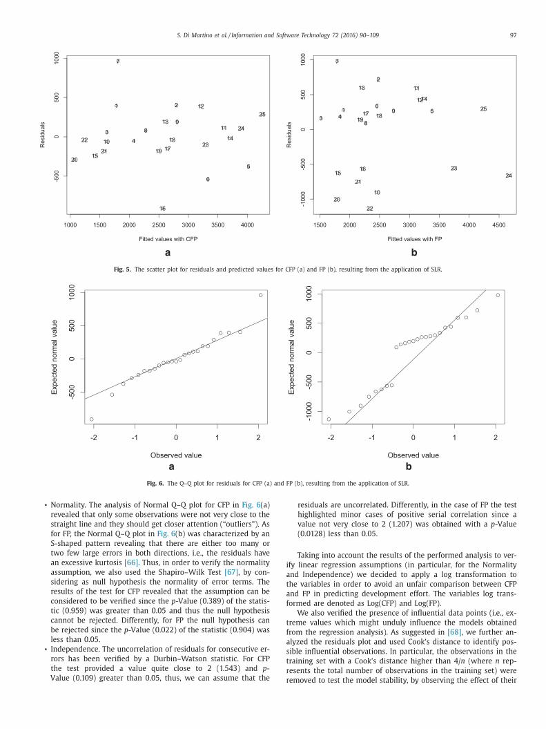
Fig. 5. The scatter plot for residuals and predicted values for CFP (a) and FP (b), resulting from the application of SLR.
-2 -1 0 1 2
-50
00
50
01
00
0
Observed value
Exp
ecte
d n
orm
al va
lue
a
-2 -1 0 1 2
-10
00
-50
00
50
01
00
0
Observed value
Exp
ecte
d n
orm
al va
lue
b
Fig. 6. The Q–Q plot for residuals for CFP (a) and FP (b), resulting from the application of SLR.
i
a
t
a
f
t
f
a
s
t
r
• Normality. The analysis of Normal Q–Q plot for CFP in Fig. 6(a)
revealed that only some observations were not very close to the
straight line and they should get closer attention (“outliers”). As
for FP, the Normal Q–Q plot in Fig. 6(b) was characterized by an
S-shaped pattern revealing that there are either too many or
two few large errors in both directions, i.e., the residuals have
an excessive kurtosis [66]. Thus, in order to verify the normality
assumption, we also used the Shapiro–Wilk Test [67], by con-
sidering as null hypothesis the normality of error terms. The
results of the test for CFP revealed that the assumption can be
considered to be verified since the p-Value (0.389) of the statis-
tic (0.959) was greater than 0.05 and thus the null hypothesis
cannot be rejected. Differently, for FP the null hypothesis can
be rejected since the p-Value (0.022) of the statistic (0.904) was
less than 0.05.
• Independence. The uncorrelation of residuals for consecutive er-
rors has been verified by a Durbin–Watson statistic. For CFP
the test provided a value quite close to 2 (1.543) and p-
Value (0.109) greater than 0.05, thus, we can assume that the
rresiduals are uncorrelated. Differently, in the case of FP the test
highlighted minor cases of positive serial correlation since a
value not very close to 2 (1.207) was obtained with a p-Value
(0.0128) less than 0.05.
Taking into account the results of the performed analysis to ver-
fy linear regression assumptions (in particular, for the Normality
nd Independence) we decided to apply a log transformation to
he variables in order to avoid an unfair comparison between CFP
nd FP in predicting development effort. The variables log trans-
ormed are denoted as Log(CFP) and Log(FP).
We also verified the presence of influential data points (i.e., ex-
reme values which might unduly influence the models obtained
rom the regression analysis). As suggested in [68], we further an-
lyzed the residuals plot and used Cook’s distance to identify pos-
ible influential observations. In particular, the observations in the
raining set with a Cook’s distance higher than 4/n (where n rep-
esents the total number of observations in the training set) were
emoved to test the model stability, by observing the effect of their
98 S. Di Martino et al. / Information and Software Technology 72 (2016) 90–109
CFP FP
-10
00
-50
00
50
01
00
0
a
CFP FP
0.5
1.0
1.5
2.0
b
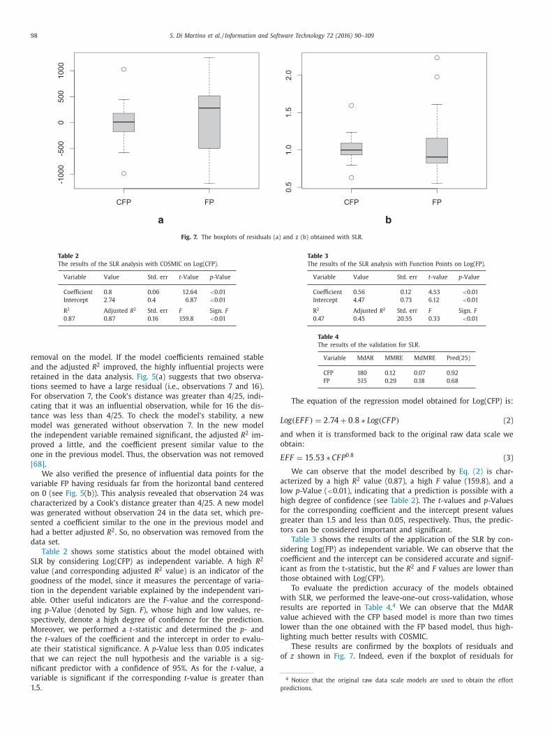
Fig. 7. The boxplots of residuals (a) and z (b) obtained with SLR.
Table 2
The results of the SLR analysis with COSMIC on Log(CFP).
Variable Value Std. err t-Value p-Value
Coefficient 0.8 0.06 12.64 <0.01
Intercept 2.74 0.4 6.87 <0.01
R2 Adjusted R2 Std. err F Sign. F
0.87 0.87 0.16 159.8 <0.01
Table 3
The results of the SLR analysis with Function Points on Log(FP).
Variable Value Std. err t-value p-Value
Coefficient 0.56 0.12 4.53 <0.01
Intercept 4.47 0.73 6.12 <0.01
R2 Adjusted R2 Std. err F Sign. F
0.47 0.45 20.55 0.33 <0.01
Table 4
The results of the validation for SLR.
Variable MdAR MMRE MdMRE Pred(25)
CFP 180 0.12 0.07 0.92
FP 515 0.29 0.18 0.68
L
a
o
E
a
l
h
f
g
t
s
c
i
t
w
r
v
l
l
o
4 Notice that the original raw data scale models are used to obtain the effort
predictions.
removal on the model. If the model coefficients remained stable
and the adjusted R2 improved, the highly influential projects were
retained in the data analysis. Fig. 5(a) suggests that two observa-
tions seemed to have a large residual (i.e., observations 7 and 16).
For observation 7, the Cook’s distance was greater than 4/25, indi-
cating that it was an influential observation, while for 16 the dis-
tance was less than 4/25. To check the model’s stability, a new
model was generated without observation 7. In the new model
the independent variable remained significant, the adjusted R2 im-
proved a little, and the coefficient present similar value to the
one in the previous model. Thus, the observation was not removed
[68].
We also verified the presence of influential data points for the
variable FP having residuals far from the horizontal band centered
on 0 (see Fig. 5(b)). This analysis revealed that observation 24 was
characterized by a Cook’s distance greater than 4/25. A new model
was generated without observation 24 in the data set, which pre-
sented a coefficient similar to the one in the previous model and
had a better adjusted R2. So, no observation was removed from the
data set.
Table 2 shows some statistics about the model obtained with
SLR by considering Log(CFP) as independent variable. A high R2
value (and corresponding adjusted R2 value) is an indicator of the
goodness of the model, since it measures the percentage of varia-
tion in the dependent variable explained by the independent vari-
able. Other useful indicators are the F-value and the correspond-
ing p-Value (denoted by Sign. F), whose high and low values, re-
spectively, denote a high degree of confidence for the prediction.
Moreover, we performed a t-statistic and determined the p- and
the t-values of the coefficient and the intercept in order to evalu-
ate their statistical significance. A p-Value less than 0.05 indicates
that we can reject the null hypothesis and the variable is a sig-
nificant predictor with a confidence of 95%. As for the t-value, a
variable is significant if the corresponding t-value is greater than
1.5.
The equation of the regression model obtained for Log(CFP) is:
og(EFF ) = 2.74 + 0.8 ∗ Log(CFP) (2)
nd when it is transformed back to the original raw data scale we
btain:
FF = 15.53 ∗ CFP0.8 (3)
We can observe that the model described by Eq. (2) is char-
cterized by a high R2 value (0.87), a high F value (159.8), and a
ow p-Value (<0.01), indicating that a prediction is possible with a
igh degree of confidence (see Table 2). The t-values and p-Values
or the corresponding coefficient and the intercept present values
reater than 1.5 and less than 0.05, respectively. Thus, the predic-
ors can be considered important and significant.
Table 3 shows the results of the application of the SLR by con-
idering Log(FP) as independent variable. We can observe that the
oefficient and the intercept can be considered accurate and signif-
cant as from the t-statistic, but the R2 and F values are lower than
hose obtained with Log(CFP).
To evaluate the prediction accuracy of the models obtained
ith SLR, we performed the leave-one-out cross-validation, whose
esults are reported in Table 4.4 We can observe that the MdAR
alue achieved with the CFP based model is more than two times
ower than the one obtained with the FP based model, thus high-
ighting much better results with COSMIC.
These results are confirmed by the boxplots of residuals and
f z shown in Fig. 7. Indeed, even if the boxplot of residuals for
S. Di Martino et al. / Information and Software Technology 72 (2016) 90–109 99
CFP FP
-15
00
-50
05
00
15
00
a
CFP FP
0.5
1.0
1.5
2.0
2.5
b
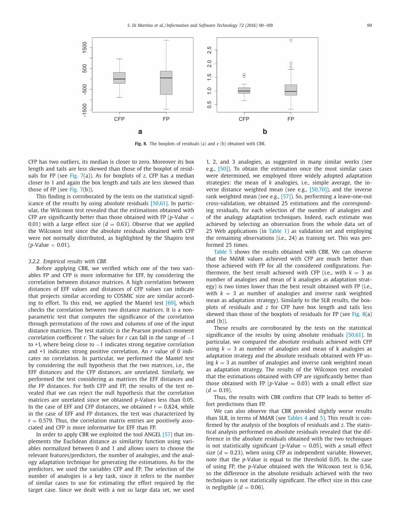
Fig. 8. The boxplots of residuals (a) and z (b) obtained with CBR.
C
l
u
c
t
i
u
C
0
t
w
(
3
a
c
d
t
i
c
p
t
d
c
t
a
c
b
E
p
t
v
m
I
i
r
c
p
a
r
o
p
n
o
t
1
e
w
s
v
r
c
i
o
a
2
t
f
t
t
t
n
e
w
m
p
s
a
s
p
u
a
i
a
t
t
(
f
t
fi
t
f
i
s
n
o
s
t
i
FP has two outliers, its median is closer to zero. Moreover its box
ength and tails are less skewed than those of the boxplot of resid-
als for FP (see Fig. 7(a)). As for boxplots of z, CFP has a median
loser to 1 and again the box length and tails are less skewed than
hose of FP (see Fig. 7(b)).
This finding is corroborated by the tests on the statistical signif-
cance of the results by using absolute residuals [50,61]. In partic-
lar, the Wilcoxon test revealed that the estimations obtained with
FP are significantly better than those obtained with FP (p-Value <
.01) with a large effect size (d = 0.63). Observe that we applied
he Wilcoxon test since the absolute residuals obtained with CFP
ere not normally distributed, as highlighted by the Shapiro test
p-Value < 0.01).
.2.2. Empirical results with CBR
Before applying CBR, we verified which one of the two vari-
bles FP and CFP is more informative for EFF, by considering the
orrelation between distance matrices. A high correlation between
istances of EFF values and distances of CFP values can indicate
hat projects similar according to COSMIC size are similar accord-
ng to effort. To this end, we applied the Mantel test [69], which
hecks the correlation between two distance matrices. It is a non-
arametric test that computes the significance of the correlation
hrough permutations of the rows and columns of one of the input
istance matrices. The test statistic is the Pearson product-moment
orrelation coefficient r. The values for r can fall in the range of −1
o +1, where being close to −1 indicates strong negative correlation
nd +1 indicates strong positive correlation. An r value of 0 indi-
ates no correlation. In particular, we performed the Mantel test
y considering the null hypothesis that the two matrices, i.e., the
FF distances and the CFP distances, are unrelated. Similarly, we
erformed the test considering as matrices the EFF distances and
he FP distances. For both CFP and FP, the results of the test re-
ealed that we can reject the null hypothesis that the correlation
atrices are unrelated since we obtained p-Values less than 0.05.
n the case of EFF and CFP distances, we obtained r = 0.824, while
n the case of EFF and FP distances, the test was characterized by
= 0.579. Thus, the correlation matrix entries are positively asso-
iated and CFP is more informative for EFF than FP.
In order to apply CBR we exploited the tool ANGEL [57] that im-
lements the Euclidean distance as similarity function using vari-
bles normalized between 0 and 1 and allows users to choose the
elevant features/predictors, the number of analogies, and the anal-
gy adaptation technique for generating the estimations. As for the
redictors, we used the variables CFP and FP. The selection of the
umber of analogies is a key task, since it refers to the number
f similar cases to use for estimating the effort required by the
arget case. Since we dealt with a not so large data set, we used
, 2, and 3 analogies, as suggested in many similar works (see
.g., [50]). To obtain the estimation once the most similar cases
ere determined, we employed three widely adopted adaptation
trategies: the mean of k analogies, i.e., simple average, the in-
erse distance weighted mean (see e.g., [50,70]), and the inverse
ank weighted mean (see e.g., [57]). So, performing a leave-one-out
ross-validation, we obtained 25 estimations and the correspond-
ng residuals, for each selection of the number of analogies and
f the analogy adaptation techniques. Indeed, each estimate was
chieved by selecting an observation from the whole data set of
5 Web applications (in Table 1) as validation set and employing
he remaining observations (i.e., 24) as training set. This was per-
ormed 25 times.
Table 5 shows the results obtained with CBR. We can observe
hat the MdAR values achieved with CFP are much better than
hose achieved with FP for all the considered configurations. Fur-
hermore, the best result achieved with CFP (i.e., with k = 3 as
umber of analogies and mean of k analogies as adaptation strat-
gy) is two times lower than the best result obtained with FP (i.e.,
ith k = 3 as number of analogies and inverse rank weighted
ean as adaptation strategy). Similarly to the SLR results, the box-
lots of residuals and z for CFP have box length and tails less
kewed than those of the boxplots of residuals for FP (see Fig. 8(a)
nd (b)).
These results are corroborated by the tests on the statistical
ignificance of the results by using absolute residuals [50,61]. In
articular, we compared the absolute residuals achieved with CFP
sing k = 3 as number of analogies and mean of k analogies as
daptation strategy and the absolute residuals obtained with FP us-
ng k = 3 as number of analogies and inverse rank weighted mean
s adaptation strategy. The results of the Wilcoxon test revealed
hat the estimations obtained with CFP are significantly better than
hose obtained with FP (p-Value = 0.03) with a small effect size
d = 0.19).
Thus, the results with CBR confirm that CFP leads to better ef-
ort predictions than FP.
We can also observe that CBR provided slightly worse results
han SLR, in terms of MdAR (see Tables 4 and 5). This result is con-
rmed by the analysis of the boxplots of residuals and z. The statis-
ical analysis performed on absolute residuals revealed that the dif-
erence in the absolute residuals obtained with the two techniques
s not statistically significant (p-Value = 0.05), with a small effect
ize (d = 0.23), when using CFP as independent variable. However,
ote that the p-Value is equal to the threshold 0.05. In the case
f using FP, the p-Value obtained with the Wilcoxon test is 0.56,
o the difference in the absolute residuals achieved with the two
echniques is not statistically significant. The effect size in this case
s negligible (d = 0.06).
100 S. Di Martino et al. / Information and Software Technology 72 (2016) 90–109
Table 5
The results of the validation for CBR.
CBR with MdAR MMRE MdMRE Pred(25)
Using CFP as predictor
k = 1; mean of k analogies 362 0.17 0.12 0.80
k = 2; mean of k analogies 245 0.16 0.12 0.80
k = 3; mean of k analogies 218 0.15 0.10 0.84
k = 1; inverse distance weighted mean 362 0.18 0.12 0.80
k = 2; inverse distance weighted mean 262 0.16 0.11 0.88
k = 3; inverse distance weighted mean 282 0.15 0.12 0.88
k = 1; inverse rank weighted mean 362 0.18 0.12 0.80
k = 2; inverse rank weighted mean 291 0.16 0.12 0.88
k = 3; inverse rank weighted mean 286 0.15 0.12 0.88
Using FP as predictor
k = 1; mean of k analogies 535 0.44 0.19 0.56
k = 2; mean of k analogies 576 0.32 0.21 0.52
k = 3; mean of k analogies 449 0.32 0.20 0.60
k = 1; inverse distance weighted mean 535 0.44 0.19 0.56
k = 2; inverse distance weighted mean 470 0.35 0.20 0.60
k = 3; inverse distance weighted mean 468 0.35 0.20 0.64
k = 1; inverse rank weighted mean 535 0.44 0.19 0.56
k = 2; inverse rank weighted mean 435 0.35 0.18 0.68
k = 3; inverse rank weighted mean 485 0.34 0.18 0.68
Table 6
Correlation among EFF and each BFC
of the COSMIC and FPA method.
BFC Rho statistic p-Value
Entry 0.823 <0.01
Exit 0.859 <0.01
Read 0.919 <0.01
Write 0.535 <0.01
EI 0.741 <0.01
EO 0.324 0.11
EQ 0.671 <0.01
ILF 0.321 0.118
EIF 0.141 0.5
Table 7
Distribution of the BFCs with respect to the final size in
terms of CFP.
FSM method Entry Exit Read Write
COSMIC 20% 19% 56% 5%
FSM method EI EO EQ ILF EIF
FPA 22% 25% 32% 10% 11%
T
B
T
w
v
p
R
a
m
i
E
I
s
T
r
n
t
t
l
t
s
E
a
s
b
4
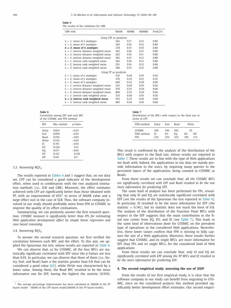
3.3. Answering RQ1a
The results reported in Tables 4 and 5 suggest that, on our data
set, CFP can be considered a good indicator of the development
effort, when used in combination with the two analyzed estima-
tion methods (i.e., SLR and CBR). Moreover, the effort estimates
achieved with CFP are significantly better than those obtained with
FP, with an improvement of 65%5 in terms of MdAR value and a
large effect size in the case of SLR. Thus, the software company in-
volved in our study should profitably move from FPA to COSMIC to
improve the quality of its effort estimations.
Summarizing, we can positively answer the first research ques-
tion: COSMIC measure is significantly better than FPs for estimating
Web application development effort by simple linear regression and
case based reasoning.
3.4. Answering RQ1b
To answer the second research question, we first verified the
correlation between each BFC and the effort. To this aim, we ap-
plied the Spearman rho test, whose results are reported in Table 6.
We can observe that, as for COSMIC, all the four BFCs are sta-
tistically significant correlated with EFF since the p-Values are less
than 0.01. In particular, we can observe that three of them (i.e., En-
try, Exit, and Read) have a rho statistic greater than 0.8 that can be
considered a good value [62], while Write was characterized by a
lower value. Among them, the Read BFC resulted to be the more
informative one for EFF, having the highest rho statistic (0.919).
5 The average percentage improvement has been calculated as (MdAR of the FP
based model – MdAR of the CFP based model)/MdAR of the FP based model).
s
M
n
his result is confirmed by the analysis of the distribution of the
FCs with respect to the final size, whose results are reported in
able 7. These results are in line with the type of Web applications
e dealt with. Indeed, the applications in our data set mainly pro-
ide information to the users, by requiring many queries to the
ersistent layers of the applications, being counted in COSMIC as
eads.
From these results we can conclude that: all the COSMIC BFCs
re significantly correlated with EFF and Read resulted to be the one
ore informative for predicting EFF.
The same kind of analysis has been performed for FPs, reveal-
ng that only EI and EQ are statistically significant correlated with
FF (see the results of the Spearman rho test reported in Table 6).
n particular, EI resulted to be the more informative for EFF (rho
tatistic = 0.741), but its statistic does not reach the level of 0.8.
he analysis of the distribution of the Function Point BFCs with
espect to the EFF suggests that the main contribution to the fi-
al size comes from EQ, EO, and EI (see Table 7). This leads to
he same kind of observations done for COSMIC on the prevalent
ype of operations in the considered Web applications. Neverthe-
ess, these lower values confirm that FPA is missing to fully cap-
ure the size of a Web application. Moreover, these results further
uggest that COSMIC, and its single BFCs, are more informative for
FF than FPs and its single BFCs, for the considered kind of Web
pplications
From these results we can conclude that: only EI and EQ are
ignificantly correlated with EFF among the FP BFCs and EI resulted to
e the more informative for predicting EFF.
. The second empirical study: assessing the use of 2SEP
From the results of our first empirical study, it is clear that the
oftware company in our study can benefit from migrating to COS-
IC, since on the considered projects this method provided sig-
ificantly better development effort estimates. Our second empiri-
S. Di Martino et al. / Information and Software Technology 72 (2016) 90–109 101
c
a
p
m
d
s
r
b
o
l
C
e
s
c
l
s
s
“
t
s
l
l
t
b
t
g
a
a
t
n
i
i
t
e
o
m
e
v
i
t
a
t
i
4
i
p
v
s
e
C
w
M
t
a
p
o
f
L
w
t
C
s
f
d
t
s
i
j
t
s
s
o
(
n
v
v
b
s
t
f
f
w
l
e
l
e
e
l
o
d
s
4
i
v
s
i
t
t
s
p
t
n
s
t
s
w
d
6 Note that we applied the procedure employed in [14] for building the conver-
sion equations exploiting the data sets that they published and in 5 cases (namely
jjcg0607 linear and non-linear, ho99 non-linear, vog03 non-linear) we found some
differences in the obtained models with respect to [14]. In the table we report the
values we obtained.
al study aims at understanding how easily this migration can be
chieved. As mentioned in the introduction of this paper, a com-
any interested in the adoption of COSMIC has to build an esti-
ation model with this measure. This basically requires historical
ata based on COSMIC that can be obtained by manually remea-
uring all the applications previously developed. This task not only
equires a lot of time, but in some cases might not even be possi-
le (e.g., due to the lack of appropriate documentation). The reuse
f data based on FPA could be very valuable to address the prob-
em, provided that there is a way to obtain the size in terms of
FPs from the size in terms of FPs. As it was pointed out by Abran
t al. [54], FPA and COSMIC measures focus on different aspects of
oftware systems since they are based on different basic functional
omponents. Thus, “exact mathematically-based conversion formu-
ae from sizes measured with a 1st generation method to COSMIC
izes are impossible”. A possible way to address the problem, also
uggested in the COSMIC documentation [54], is to search for some
statistically-based conversion formulae”.
Some researchers have been investigating the suitability and
he effectiveness of such an approach by trying to build conver-
ion equations for different data sets. In particular, linear and non-
inear equations have been built on the raw data and on the
og-transformed data, respectively [14]. Also, more sophisticated
echniques, such as piecewise regression, have been employed for
uilding non-linear models [15].
The results reported in the literature [14,15,22,23,71–75] reveal
hat a statistical conversion is possible, thus supporting the sug-
estions provided in the COSMIC documentation [54]. The studies
lso showed that both linear and non-linear models should be an-
lyzed to identify the best correlation. Furthermore, more complex
echniques, such as piecewise regression [15]), did not provide sig-
ificantly better results, being at the same time hardly applicable.
The aim of our second empirical study was to analyze whether
t is possible to reuse the FP → CFP conversion equations proposed
n the literature (i.e., external conversion equations) to apply the
wo-step process shown in Fig. 1 (named 2SEP) for building effort
stimation models. In other words, we assessed if, given the size
f past projects in terms of FPs, it is possible to convert them by
eans of some equations into COSMIC measure to build an effort
stimation model. Furthermore, we also considered the use of con-
ersion equations built on a (small) data set of the company taken
nto account (i.e., internal conversion equations).
In the following, before presenting the design (Section 4.3) and
he results (Section 4.4) of our second empirical study, we provide
brief description of the external conversion equations we decided
o employ (Section 4.1) and we describe the construction of the
nternal conversion equations (Section 4.2).
.1. External conversion equations from previous studies
In our study we took into account the results of two previous
nvestigations that analyzed the relationship between the sizes ex-
ressed in terms of FPs and of CFPs, namely [14] and [76].
The aim of Cuadrado-Gallego et al. [14] was to carry out a re-
iew of previous investigations that mainly exploited linear regres-
ion analysis for converting FPs into CFPs, i.e., by constructing an
quation as:
FPFP = a + b ∗ FP (4)
here the dependent variable CFPFP represents the estimated COS-
IC size and the independent variable FP represents the size in
erms of FPs.
Moreover, Cuadrado-Gallego et al. were also the first to propose
n analysis on a non-linear relation between CFPFP and FP, by ex-
loiting the log transformation of the variables in the application
f linear regression analysis. Thus, the equation obtained is of this
orm:
og(CFPFP) = Log(a) + b ∗ Log(FP) (5)
hich, when transformed back to the original raw data scale, gives
he equation:
FPFP = a ∗ FPb (6)
For the evaluation, they employed nine publicly available data
ets: six of them were obtained from previous studies (i.e., named
et99 [77], fet99-2 [78], ho99 [72], vog03 [78], abr05 [22], and
es06[23]). Three additional data sets were included in the paper:
he first two (named jjcg06 and jjcg07) contained 21 and 14 ob-
ervations, respectively, and were obtained in two different stud-
es conducted with academic students, while the third one (named
jcg0607) was obtained by merging the first two.
The parameters of the linear and non-linear conversion equa-
ions obtained for the above data sets are reported in Table 8,6 re-
pectively. In particular, the tables show, for each employed data
et, the equation parameters a and b, and the R2 value. We can
bserve that the linear conversion equations reported in Table 8
top) are characterized by a coefficient quite close to 1, and the
on-linear equations (see Table 8 (bottom)) have the coefficient
alues even closer to 1. These results seem to suggest that a con-
ersion equation based on the assumption of 1 CFP ∼= 1 FP could
e possible. Cuadrado-Gallego et al. argued that a 1 to 1 conver-
ion factor cannot be attributed to anything other than an influen-
ial coincidence. Indeed, even if both FPA and COSMIC measure the
unctional size of the software, they are taking in consideration dif-
erent characteristics and also different counting procedures. [14].
Lavazza [76] also exploited some of the data used in previous
ork [14,48] to empirically assess and compare linear and non-
inear models against Piecewise Linear Regression, with a special
mphasis on the role of outliers. He built 6 linear and 6 non-
inear models, whose information can be found in Table 9. These
quations differ from the one in the work of Cuadrado-Gallego
t al. [14] since Lavazza eliminated from the data sets the out-
iers affecting the models. As already mentioned at the beginning
f Section 4, we did not consider the Piecewise Regression since it
id not provide significantly better results than SLR, being at the
ame time hardly applicable [15].
.2. Internal conversion equations built on our data set
To build internal conversion equations with SLR we first ver-
fied the relationship between the dependent and independent
ariables CFP and FP, respectively, by assessing linear regres-
ion assumptions, i.e., linearity, homoscedasticity, normality, and
ndependence. In particular, the Spearman’ rho test revealed that
here was a positive linear relationship between CFP and FP (statis-
ic = 0.848 with p-Value < 0.01), while the Breush–Pagan Test
howed that homoscedasticity assumption was verified since the
-Value (0.674) of the statistic (0.176) was greater than 0.05. On
he other hand, the normality assumption for the residuals can-
ot be considered to be verified since the p-Value (0.243) of the
tatistic (0.949) was greater than 0.05. As for the independence,
he Durbin–Watson statistic was not close to 2 (1.34). As a con-
equence, we also applied a log-transformation of the data and
e considered both linear and non-linear conversion equations as
one in previous investigations (e.g., [14,76]).
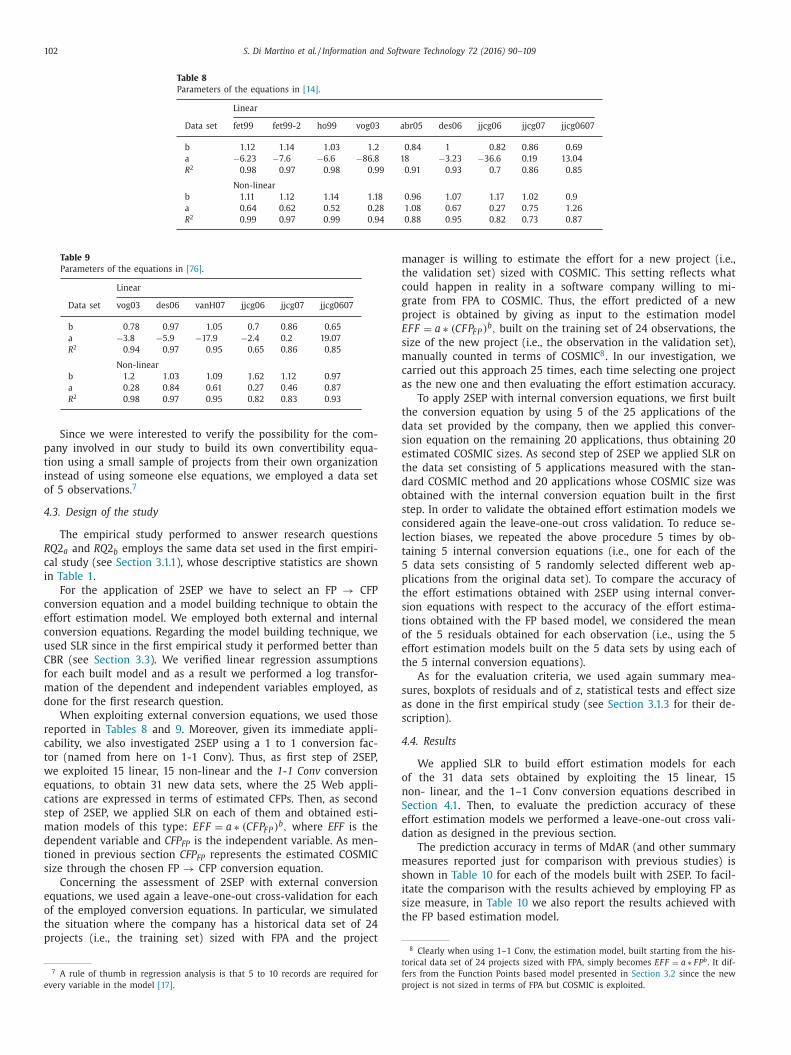
102 S. Di Martino et al. / Information and Software Technology 72 (2016) 90–109
Table 8
Parameters of the equations in [14].
Linear
Data set fet99 fet99-2 ho99 vog03 abr05 des06 jjcg06 jjcg07 jjcg0607
b 1.12 1.14 1.03 1.2 0.84 1 0.82 0.86 0.69
a −6.23 −7.6 −6.6 −86.8 18 −3.23 −36.6 0.19 13.04
R2 0.98 0.97 0.98 0.99 0.91 0.93 0.7 0.86 0.85
Non-linear
b 1.11 1.12 1.14 1.18 0.96 1.07 1.17 1.02 0.9
a 0.64 0.62 0.52 0.28 1.08 0.67 0.27 0.75 1.26
R2 0.99 0.97 0.99 0.94 0.88 0.95 0.82 0.73 0.87
Table 9
Parameters of the equations in [76].
Linear
Data set vog03 des06 vanH07 jjcg06 jjcg07 jjcg0607
b 0.78 0.97 1.05 0.7 0.86 0.65
a −3.8 −5.9 −17.9 −2.4 0.2 19.07
R2 0.94 0.97 0.95 0.65 0.86 0.85
Non-linear
b 1.2 1.03 1.09 1.62 1.12 0.97
a 0.28 0.84 0.61 0.27 0.46 0.87
R2 0.98 0.97 0.95 0.82 0.83 0.93
m
t
c
g
p
E
s
m
c
a
t
d
s
e
t
d
o
s
c
l
t
5
p
t
s
t
o
e
t
s
a
s
4
o
n
S
e
d
m
s
i
s
t
Since we were interested to verify the possibility for the com-
pany involved in our study to build its own convertibility equa-
tion using a small sample of projects from their own organization
instead of using someone else equations, we employed a data set
of 5 observations.7
4.3. Design of the study
The empirical study performed to answer research questions
RQ2a and RQ2b employs the same data set used in the first empiri-
cal study (see Section 3.1.1), whose descriptive statistics are shown
in Table 1.
For the application of 2SEP we have to select an FP → CFP
conversion equation and a model building technique to obtain the
effort estimation model. We employed both external and internal
conversion equations. Regarding the model building technique, we
used SLR since in the first empirical study it performed better than
CBR (see Section 3.3). We verified linear regression assumptions
for each built model and as a result we performed a log transfor-
mation of the dependent and independent variables employed, as
done for the first research question.
When exploiting external conversion equations, we used those
reported in Tables 8 and 9. Moreover, given its immediate appli-
cability, we also investigated 2SEP using a 1 to 1 conversion fac-
tor (named from here on 1-1 Conv). Thus, as first step of 2SEP,
we exploited 15 linear, 15 non-linear and the 1-1 Conv conversion
equations, to obtain 31 new data sets, where the 25 Web appli-
cations are expressed in terms of estimated CFPs. Then, as second
step of 2SEP, we applied SLR on each of them and obtained esti-
mation models of this type: EFF = a ∗ (CFPFP)b, where EFF is the
dependent variable and CFPFP is the independent variable. As men-
tioned in previous section CFPFP represents the estimated COSMIC
size through the chosen FP → CFP conversion equation.
Concerning the assessment of 2SEP with external conversion
equations, we used again a leave-one-out cross-validation for each
of the employed conversion equations. In particular, we simulated
the situation where the company has a historical data set of 24
projects (i.e., the training set) sized with FPA and the project
7 A rule of thumb in regression analysis is that 5 to 10 records are required for
every variable in the model [17].
t
f
p
anager is willing to estimate the effort for a new project (i.e.,
he validation set) sized with COSMIC. This setting reflects what
ould happen in reality in a software company willing to mi-
rate from FPA to COSMIC. Thus, the effort predicted of a new
roject is obtained by giving as input to the estimation model
FF = a ∗ (CFPFP)b, built on the training set of 24 observations, the
ize of the new project (i.e., the observation in the validation set),
anually counted in terms of COSMIC8. In our investigation, we
arried out this approach 25 times, each time selecting one project
s the new one and then evaluating the effort estimation accuracy.
To apply 2SEP with internal conversion equations, we first built
he conversion equation by using 5 of the 25 applications of the
ata set provided by the company, then we applied this conver-
ion equation on the remaining 20 applications, thus obtaining 20
stimated COSMIC sizes. As second step of 2SEP we applied SLR on
he data set consisting of 5 applications measured with the stan-
ard COSMIC method and 20 applications whose COSMIC size was
btained with the internal conversion equation built in the first
tep. In order to validate the obtained effort estimation models we
onsidered again the leave-one-out cross validation. To reduce se-
ection biases, we repeated the above procedure 5 times by ob-
aining 5 internal conversion equations (i.e., one for each of the
data sets consisting of 5 randomly selected different web ap-
lications from the original data set). To compare the accuracy of
he effort estimations obtained with 2SEP using internal conver-
ion equations with respect to the accuracy of the effort estima-
ions obtained with the FP based model, we considered the mean
f the 5 residuals obtained for each observation (i.e., using the 5
ffort estimation models built on the 5 data sets by using each of
he 5 internal conversion equations).
As for the evaluation criteria, we used again summary mea-
ures, boxplots of residuals and of z, statistical tests and effect size
s done in the first empirical study (see Section 3.1.3 for their de-
cription).
.4. Results
We applied SLR to build effort estimation models for each
f the 31 data sets obtained by exploiting the 15 linear, 15
on- linear, and the 1–1 Conv conversion equations described in
ection 4.1. Then, to evaluate the prediction accuracy of these
ffort estimation models we performed a leave-one-out cross vali-
ation as designed in the previous section.
The prediction accuracy in terms of MdAR (and other summary
easures reported just for comparison with previous studies) is
hown in Table 10 for each of the models built with 2SEP. To facil-
tate the comparison with the results achieved by employing FP as
ize measure, in Table 10 we also report the results achieved with
he FP based estimation model.
8 Clearly when using 1–1 Conv, the estimation model, built starting from the his-
orical data set of 24 projects sized with FPA, simply becomes EFF = a ∗ FPb. It dif-
ers from the Function Points based model presented in Section 3.2 since the new
roject is not sized in terms of FPA but COSMIC is exploited.
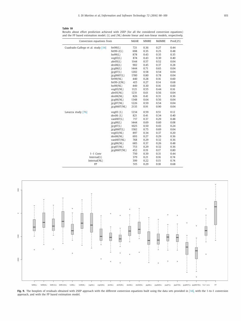
S. Di Martino et al. / Information and Software Technology 72 (2016) 90–109 103
Table 10
Results about effort prediction achieved with 2SEP (for all the considered conversion equations)
and the FP based estimation model. (L) and (NL) denote linear and non-linear models, respectively.
Conversion equations from MdAR MMRE MdMRE Pred(25)
Cuadrado-Gallego et al. study [14] fet99(L) 721 0.36 0.27 0.44
fet99-2(L) 698 0.35 0.25 0.48
ho99(L) 878 0.43 0.35 0.35
vog03(L) 874 0.43 0.30 0.40
abr05(L) 1144 0.57 0.52 0.04
des06(L) 902 0.45 0.37 0.28
jjcg06(L) 1444 0.71 0.65 0.04
jjcg07(L) 1202 0.58 0.54 0.04
jjcg0607(L) 1780 0.80 0.78 0.04
fet99(NL) 440 0.28 0.16 0.60
fet99-2(NL) 415 0.27 0.14 0.68
ho99(NL) 449 0.30 0.16 0.60
vog03(NL) 1121 0.55 0.44 0.16
abr05(NL) 1231 0.61 0.56 0.04
des06(NL) 826 0.41 0.31 0.36
jjcg06(NL) 1348 0.64 0.56 0.04
jjcg07(NL) 1226 0.59 0.54 0.04
jjcg0607(NL) 2135 0.91 0.90 0.04
Lavazza study [76] vog03 (L) 1234 0.59 0.51 0.12
des06 (L) 821 0.41 0.34 0.40
vanH07(L) 717 0.37 0.29 0.48
jjcg06(L) 1444 0.69 0.60 0.08
jjcg07(L) 1025 0.50 0.43 0.24
jjcg0607(L) 1582 0.75 0.69 0.04
vog03(NL) 897 0.34 0.37 0.20
des06(NL) 693 0.27 0.29 0.36
vanH07(NL) 768 0.29 0.32 0.36
jjcg06(NL) 685 0.37 0.26 0.48
jjcg07(NL) 753 0.29 0.32 0.36
jjcg0607(NL) 452 0.19 0.17 0.80
1–1 Conv 750 0.39 0.31 0.44
Internal(L) 379 0.21 0.16 0.74
Internal(NL) 399 0.22 0.15 0.74
FP 515 0.29 0.18 0.68
fet99(L) fet99(NL) fet99-2(L) fet99-2(NL) ho99(L) ho99(NL) vog03(L) vog03(NL) abr05(L) abr05(NL) des06(L) des06(NL) jjcg06(L) jjcg06(NL) jjcg07(L) jjcg07(NL) jjcg0607(L) jjcg0607(NL) 1-to-1 conv FP
-20
00
-10
00
01
00
0
Fig. 9. The boxplots of residuals obtained with 2SEP approach with the different conversion equations built using the data sets provided in [14], with the 1-to-1 conversion
approach, and with the FP based estimation model.
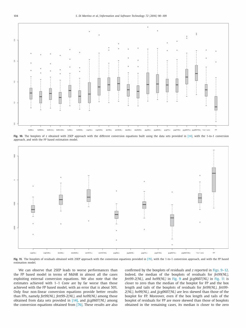
104 S. Di Martino et al. / Information and Software Technology 72 (2016) 90–109
fet99(L) fet99(NL) fet99-2(L) fet99-2(NL) ho99(L) ho99(NL) vog03(L) vog03(NL) abr05(L) abr05(NL) des06(L) des06(NL) jjcg06(L) jjcg06(NL) jjcg07(L) jjcg07(NL) jjcg0607(L) jjcg0607(NL) 1-to-1 conv FP
0.5
1.0
1.5
2.0
2.5
Fig. 10. The boxplots of z obtained with 2SEP approach with the different conversion equations built using the data sets provided in [14], with the 1-to-1 conversion
approach, and with the FP based estimation model.
vog03(L) vog03(NL) des06(L) des06(NL) vanH07(L) vanH07(NL) jjcg06(L) jjcg06(NL) jjcg07(L) jjcg07(NL) jjcg0607(L) jjcg0607(NL) 1-to-1 conv FP
-20
00
-10
00
01
00
0
Fig. 11. The boxplots of residuals obtained with 2SEP approach with the conversion equations provided in [76], with the 1-to-1 conversion approach, and with the FP based
estimation model.
c
I
f
c
l
2
b
b
o
We can observe that 2SEP leads to worse performances than
the FP based model in terms of MdAR in almost all the cases
exploiting external conversion equations. We also note that the
estimates achieved with 1–1 Conv are by far worse than those
achieved with the FP based model, with an error that is about 50%.
Only four non-linear conversion equations provide better results
than FPs, namely fet99(NL), fett99-2(NL), and ho99(NL) among those
obtained from data sets provided in [14], and jjcg0607(NL) among
the conversion equations obtained from [76]. These results are also
onfirmed by the boxplots of residuals and z reported in Figs. 9–12.
ndeed, the median of the boxplots of residuals for fet99(NL),
ett99-2(NL), and ho99(NL) in Fig. 9 and jjcg0607(NL) in Fig. 11 is
loser to zero than the median of the boxplot for FP and the box
ength and tails of the boxplots of residuals for fet99(NL), fett99-
(NL), ho99(NL), and jjcg0607(NL) are less skewed than those of the
oxplot for FP. Moreover, even if the box length and tails of the
oxplot of residuals for FP are more skewed than those of boxplots
btained in the remaining cases, its median is closer to the zero
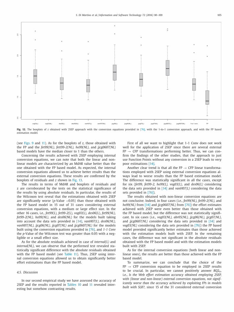
S. Di Martino et al. / Information and Software Technology 72 (2016) 90–109 105
vog03(L) vog03(NL) des06(L) des06(NL) vanH07(L) vanH07(NL) jjcg06(L) jjcg06(NL) jjcg07(L) jjcg07(NL) jjcg0607(L) jjcg0607(NL) 1-to-1 conv FP
0.5
1.0
1.5
2.0
2.5
Fig. 12. The boxplots of z obtained with 2SEP approach with the conversion equations provided in [76], with the 1-to-1 conversion approach, and with the FP based
estimation model.
(
t
b
c
l
o
c
e
b
z
t
t
a
t
c
o
f
i
v
b
t
l
i
t
w
n
e
4
2
e
w
F
fi
u
p
t
w
T
f
t
s
n
h
a
t
c
a
v
m
w
c
o
b
l
b
F
t
i
w
i
b
see Figs. 9 and 11). As for the boxplots of z, those obtained with
he FP and the fet99(NL), fett99-2(NL), ho99(NL), and jjcg0607(NL)
ased models have the median closer to 1 than the others.
Concerning the results achieved with 2SEP employing internal
onversion equations, we can note that both the linear and non-
inear models are characterized by an MdAR value better than the
ne obtained with the FP based model. As expected, the internal
onversion equations allowed us to achieve better results than the
xternal conversion equations. These results are confirmed by the
oxplots of residuals and z shown in Fig. 13.
The results in terms of MdAR and boxplots of residuals and
are corroborated by the tests on the statistical significance of
he results by using absolute residuals. In particular, the results of
he Wilcoxon test reveal that the estimations obtained with 2SEP
re significantly worse (p-Value <0.05) than those obtained with
he FP based model in 15 out of 31 cases considering external
onversion equations, with a medium or large effect size. In the
ther 16 cases, i.e., fet99(L), fet99-2(L), vog03(L), des06(L), fet99(NL),
et99-2(NL), ho99(NL), and des06(NL) for the models built taking
nto account the data sets provided in [14], vanH07(L), des06(NL),
anH07(NL), jjcg06(NL), jjcg07(NL) and jjcg0607(NL) for the models
uilt using the conversion equations provided in [76], and 1-1 Conv
he p-Value of the Wilcoxon test was greater than 0.05 with a neg-
igible or a small effect size.
As for the absolute residuals achieved in case of internal(L) and
nternal(NL), we can observe that the performed test revealed sta-
istically significant difference with the absolute residuals obtained
ith the FP based model (see Table 11). Thus, 2SEP using inter-
al conversion equations allowed us to obtain significantly better
ffort estimations than the FP based model.
.5. Discussion
In our second empirical study we have assessed the accuracy of
SEP and the results reported in Tables 10 and 11 revealed inter-
sting but somehow contrasting results.
First of all we want to highlight that 1-1 Conv does not work
ell for the application of 2SEP since there are several external
P → CFP transformations performing better. Thus, we can con-
rm the findings of the other studies, that the approach to just
se Function Points without any conversion in a 2SEP leads to very
oor estimations [14].
Another clear trend is that all the FP → CFP linear transforma-
ions employed with 2SEP using external conversion equations al-
ays lead to worse results than the FP based estimation model.
he difference was statistically significant in all the cases, except
or six (fet99, fet99-2, ho99(L), vog03(L), and des06(L) considering
he data sets provided in [14] and vanH07(L) considering the data
ets provided in [76]).
The results obtained with non-linear conversion equations are
ot conclusive. Indeed, in four cases (i.e., fet99(NL), fet99-2(NL), and
o99(NL) from [14] and jjcg0607(NL) from [76]) the effort estimates
chieved with 2SEP were even better than those obtained with
he FP based model, but the difference was not statistically signifi-
ant. In six cases (i.e., vog03(NL), abr05(NL), jjcg06(NL), jjcg07(NL),
nd jjcg0607(NL) considering the data sets provided in [14] and
og03(NL) considering the data sets provided in [76]) the FP based
odel provided significantly better estimates than those achieved
ith the estimation models built with 2SEP. In the remaining
ases, the difference was not significant in the absolute residuals
btained with the FP based model and with the estimation models
uilt with 2SEP.
As for the internal conversion equations (both linear and non-
inear ones), the results are better than those achieved with the FP
ased model.
To summarize, we can conclude that the choice of the
P → CFP conversion equation to be employed in 2SEP results
o be crucial. In particular, we cannot positively answer RQ2a,
.e., Is the Web effort estimation accuracy obtained employing 2SEP,
ith (linear and non-linear) external conversion equations, not signif-
cantly worse than the accuracy achieved by exploiting FPs in models
uilt with SLR?, since 15 of the 31 considered external conversion
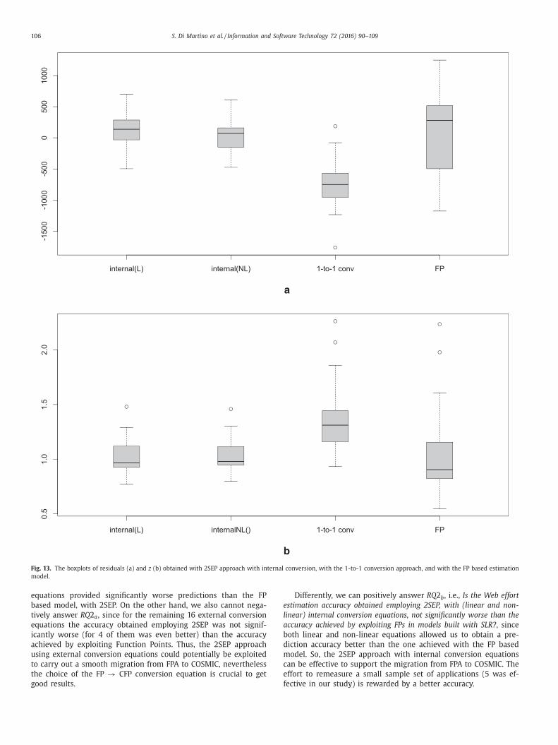
106 S. Di Martino et al. / Information and Software Technology 72 (2016) 90–109
internal(L) internal(NL) 1-to-1 conv FP
-15
00
-10
00
-50
00
50
01
00
0
a
internal(L) internalNL() 1-to-1 conv FP
0.5
1.0
1.5
2.0
b
Fig. 13. The boxplots of residuals (a) and z (b) obtained with 2SEP approach with internal conversion, with the 1-to-1 conversion approach, and with the FP based estimation
model.
e
l
a
b
d
m
c
e
f
equations provided significantly worse predictions than the FP
based model, with 2SEP. On the other hand, we also cannot nega-
tively answer RQ2a, since for the remaining 16 external conversion
equations the accuracy obtained employing 2SEP was not signif-
icantly worse (for 4 of them was even better) than the accuracy
achieved by exploiting Function Points. Thus, the 2SEP approach
using external conversion equations could potentially be exploited
to carry out a smooth migration from FPA to COSMIC, nevertheless
the choice of the FP → CFP conversion equation is crucial to get
good results.
Differently, we can positively answer RQ2b, i.e., Is the Web effort
stimation accuracy obtained employing 2SEP, with (linear and non-
inear) internal conversion equations, not significantly worse than the
ccuracy achieved by exploiting FPs in models built with SLR?, since
oth linear and non-linear equations allowed us to obtain a pre-
iction accuracy better than the one achieved with the FP based
odel. So, the 2SEP approach with internal conversion equations
an be effective to support the migration from FPA to COSMIC. The
ffort to remeasure a small sample set of applications (5 was ef-
ective in our study) is rewarded by a better accuracy.
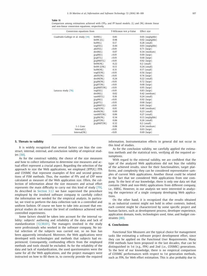
S. Di Martino et al. / Information and Software Technology 72 (2016) 90–109 107
Table 11
Comparison among estimations achieved with CFPFP and FP based models. (L) and (NL) denote linear
and non-linear conversion equations, respectively.
Conversion equations from T-Wilcoxon test p-Value Effect size
Cuadrado-Gallego et al. study [14] fet99(L) 0.85 0.05 (negligible)
fet99-2(L) 0.98 0.02 (negligible)
ho99(L) 0.17 0.28 (small)
vog03(L) 0.44 0.03 (negligible)
abr05(L) <0.01 0.71 (large)
des06(L) 0.07 0.34 (medium)
jjcg06(L) <0.01 0.69 (large)
jjcg07(L) <0.01 0.68 (large)
jjcg0607(L) <0.01 0.92 (large)
fet99(NL) 0.22 0.2 (small)
fet99-2(NL) 0.13 0.24 (small)
ho99(NL) 0.31 0.17 (small)
vog03(NL) <0.01 0.56 (large)
abr05(NL) <0.01 0.74 (large)
des06(NL) 0.24 0.22 (small)
jjcg06(NL) <0.01 0.72 (large)
jjcg07(NL) <0.01 0.68 (large)
jjcg0607(NL) <0.01 0.95 (large)
Lavazza study [76] vog03(L) <0.01 0.83 (large)
des06(L) 0.02 0.42 (medium)
vanH07(L) 0.18 0.24 (small)
jjcg06(L) <0.01 0.92 (large)
jjcg07(L) <0.01 0.68 (large)
jjcg0607(L) <0.01 0.95 (large)
vog03(NL) 0.01 0.40 (medium)
des06(NL) 0.09 0.23 (small)
vanH07(NL) 0.06 0.27 (small)
jjcg06(NL) 0.34 0.13 (negligible)
jjcg07(NL) 0.06 0.26 (small)
jjcg0607(NL) 0.32 0.2 (small)
1-1 Conv 0.08 0.34 (medium)
Internal(L) <0.01 0.63 (large)
Internal(NL) <0.01 0.69 (large)
5
s
i
a
t
a
a
t
c
l
r
A
e
t
l
u
p
c
l
s
w
t
b
d
p
m
d
s
i
i
t
t
s
t
o
f
p
t
p
c
i
i
t
i
e
h
a
s
6
t
t
F
d
T
o
. Threats to validity
It is widely recognized that several factors can bias the con-
truct, internal, external, and conclusion validity of empirical stud-
es [50].
As for the construct validity, the choice of the size measures
nd how to collect information to determine size measures and ac-
ual effort represent a crucial aspect. Regarding the selection of the
pproach to size the Web applications, we employed (IFPUG) FPA
nd COSMIC that represent examples of first and second genera-
ions of FSM methods. Thus, the number of FPs and of CFP were
alculated as measure of the Web application size. Often, the col-
ection of information about the size measures and actual effort
epresents the main difficulty to carry out this kind of study [79].
s described in Section 3.1.1 we have supervised the procedure
mployed by the involved software company to carefully collect
he information we needed for the empirical analysis. In particu-
ar, we tried to perform the data collection task in a controlled and
niform fashion. Of course we have to take into account that em-
irical studies do not ensure the level of confidence achieved with
ontrolled experiments.
Some factors should be taken into account for the internal va-
idity: subjects’ authoring and reliability of the data and lack of
tandardization [12,50,61]. The managers involved in the study
ere professionals who worked in the software company. No ini-
ial selection of the subjects was carried out, so no bias has
een apparently introduced. Moreover, the Web applications were
eveloped with technologies and methods that subjects had ex-
erienced. Consequently, confounding effects from the employed
ethods and tools should be excluded. As for the reliability of the
ata and lack of standardization, the used questionnaires were the
ame for all the Web applications, and the project managers were
nstructed on how to fill them in, to correctly provide the required
snformation. Instrumentation effects in general did not occur in
his kind of studies.
As for the conclusion validity, we carefully applied the estima-
ion methods and the statistical tests, verifying all the required as-
umptions.
With regard to the external validity, we are confident that the
ype of the analyzed Web applications did not bias the validity
f the achieved results, since for their functionalities, target plat-
orms, and complexity they can be considered representative sam-
les of current Web applications. Another threat could be related
o the fact that we considered Web applications from one com-
any. To the best of our knowledge, there is only one data set that
ontains (Web and non-Web) applications from different company,
.e., ISBSG. However, in our analysis we were interested in analyz-
ng the experience of a single company developing Web applica-
ions.
On the other hand, it is recognized that the results obtained
n an industrial context might not hold in other contexts. Indeed,
ach context might be characterized by some specific project and
uman factors, such as development process, developer experience,
pplication domain, tools, technologies used, time, and budget con-
traints [80].
. Conclusions
Functional Size Measures are the typical choice for management
asks like estimating a software project development effort, since
hey can be applied on the Functional User Requirements. Many
SM methods have been proposed in the last decades, that can be
istinguished in 1st (e.g., FPA) and 2nd (i.e., COSMIC) generations.
o the best of our knowledge, there is no empirical comparison
f COSMIC performances with respect to 1st generation methods,
uch as FPA, for Web effort estimation. This is also probably due to
108 S. Di Martino et al. / Information and Software Technology 72 (2016) 90–109
the lack of suitable industrial data sets containing information on
Web application measured with both FPA and COSMIC. The main
goal of our work was to empirically investigate whether COSMIC
is more effective than FPA for Web effort estimation, thus moti-
vating the migration from 1st generation FSM methods to the 2nd
one. We were also interested in investigating the effectiveness of
an approach to facilitate the migration from FPA to COSMIC. Com-
panies could apply a two-step estimation process (2SEP) that ex-
ploits historical FPA data and a conversion equation to estimate
COSMIC sizes and use them to predict development effort, until
enough COSMIC data has been collected. In the case they would
not spend effort and time in resizing historical projects in terms of
COSMIC, to be used for effort estimation, they could employ exter-
nal conversion equations, otherwise they could remeasure a small
sample data set in terms of COSMIC and build an internal conver-
sion equation.
We performed two empirical studies, both exploiting data from
25 industrial Web applications, and employing leave-one-out cross
validation as validation method.
The results of the first empirical study revealed that COSMIC
outperformed Function Points as indicator of development effort
by providing significantly better estimations, when used in com-
bination with two different estimation techniques (SLR and CBR).
Thus, for the software company involved in our empirical study,
the decision of migrating from FPA to COSMIC is positively sup-
ported by the results of the study presented here.
The results of the second empirical study revealed that the 2SEP
approach could potentially be exploited to carry out a migration
from FPA to COSMIC. Anyhow, the choice of the FP → CFP con-
version equation is crucial to achieve good results. As expected,
the internal conversion equations allowed us to obtain effort pre-
dictions better than those achieved employing external conversion
equations. However, employing internal conversion equations re-
quires re-measuring a sample of previous developed applications,
i.e., further effort by managers of the company. As for external
conversion equations, more investigations should be carried out to
identify more accurate conversion equations possibly relating them
to specific types of software systems.
The experimental results presented herein hold for the com-
pany involved in our study and they should be assessed on further
data as soon as it becomes available. We have planned to collect
information from other companies, operating also in other indus-
trial contexts, in order to compare the accuracy of COSMIC and FPs
for Web effort estimation and assess a two-step process for build-
ing effort estimation models.
References
[1] I. Sommerville, Software Engineering, ninth ed., Addison-Wesley, Harlow, Eng-
land, 2010.
[2] A. Albrecht, Measuring application development productivity, in: Proceedingsof the Joint SHARE/GUIDE/IBM Application Development Symposium, 1979,
pp. 83–92.[3] Ç. Gencel, O. Demirörs, Functional size measurement revisited, ACM Trans.
Softw. Eng. Methodol. 17 (3) (2008).[4] ISO, ISO/IEC 14143-1:2007: Information Technology – Software measurement –
Functional Size Measurement, 2007.
[5] A. Abran, J. Desharnais, A. Lesterhuis, B. Londeix, R. Meli, P. Morris, S. Oligny,M. ONeil, T. Rollo, G. Rule, L. Santillo, C. Symons, H. Toivonen, The COS-
MIC Functional Size Measurement Method Measurement Manual, version 4.0.1,2015.
[6] T. Rollo, Sizing e-commerce, in: Proceedings of Australian Conference on Soft-ware Measurement, IEEE Press, 2000.
[7] S. Abraháo, O. Pastor, Measuring the functional size of Web applications, Int. J.Web Eng. Technol. 1 (1) (2003) 5–16.
[8] P. Fraternali, M. Tisi, A. Bongio, Automating function point analysis with model
driven development, in: Proceedings of conference of the Center for AdvancedStudies on Collaborative research, 2006, pp. 233–247.
[9] G. Costagliola, S. Di Martino, F. Ferrucci, C. Gravino, G. Tortora, G. Vitiello, ACOSMIC-FFP approach to predict Web application development effort, J. Web
Eng. 5 (2) (2006) 93–120.
[10] S. Di Martino, F. Ferrucci, C. Gravino, Estimating Web application developmenteffort using Web-COBRA and COSMIC: an empirical study, in: Proceedings of
Euromicro Conference on Software Engineering and Advanced Applications,ACM Press, 2009, pp. 306–312.
[11] F. Ferrucci, C. Gravino, S. Di Martino, A case study using Web Objects and COS-MIC for effort estimation of Web applications, in: Proceedings of Euromicro
Conference on Software Engineering and Advanced Applications, IEEE Press,2008, pp. 441–448.
[12] E. Mendes, S. Counsell, N. Mosley, Comparison of Web size measures for pre-
dicting Web design and authoring effort, IEE Proc.–Softw. 149 (3) (2002) 86–92.
[13] S. Di Martino, C. Gravino, Estimating Web application development effort usingCOSMIC-FFP method, Int. J. Comput. Appl. 31 (3) (2009).
[14] J.J. Cuadrado-Gallego, L. Buglione, M.J. Domínguez-Alda, M.F.d. Sevilla, J. Anto-nio Gutierrez de Mesa, O. Demirors, An experimental study on the conversion
between IFPUG and COSMIC functional size measurement units, Inf. Softw.
Technol. 52 (3) (2010) 347–357.[15] L. Lavazza, S. Morasca, Convertibility of function points into COSMIC function
points: a study using piecewise linear regression, Inf. Softw. Technol. 53 (8)(2011) 874–884.
[16] L. Buglione, F. Ferrucci, C. Gencel, C. Gravino, F. Sarro, Which COSMIC basefunctional components are significant in estimating web application develop-
ment? – a case study, in: Proceedings of International Conference on Software
Process and Product Measurement, 2010, pp. 205–224.[17] T. Menzies, Z. Chen, J. Hihn, K. Lum, Selecting best practices for effort estima-
tion, IEEE Trans. Softw. Eng. 32 (11) (2006) 883–895.[18] A. Corazza, S. Di Martino, F. Ferrucci, C. Gravino, F. Sarro, E. Mendes, Using
tabu search to configure support vector regression for effort estimation, Empir.Softw. Eng. 18 (3) (2013) 506–546.
[19] A. Corazza, S. Di Martino, F. Ferrucci, C. Gravino, E. Mendes, Investigating the
use of support vector regression for Web effort estimation, Empir. Softw. Eng.16 (2) (2011) 211–243.
[20] F. Ferrucci, M. Harman, F. Sarro, Search-Based Software Project Management,in: Software Project Management in a Changing World, Springer Berlin Hei-
delberg, 2014, pp. 373–399.[21] E. Kocaguneli, T. Menzies, J.W. Keung, On the value of ensemble effort estima-
tion, IEEE Trans. Softw. Eng. 38 (6) (2012) 1403–1416.
[22] A. Abran, J. Desharnais, F. Azziz, Measurement convertibility: from functionpoints to COSMIC, in: Proceedings of the International Workshop on Software
Measurement, Shaker-Verlag, 2005, p. 227240.[23] J. Desharnais, A. Abran, J. Cuadrado-Gallego, Convertibility of function points
to COSMIC: identification and analysis of functional outliers, in: Proceedingsof the International Workshop on Software Measurement, Shaker-Verlag, 2007,
p. 130-146.
[24] H. Zuse, A Framework of Software Measurement, Walter de Gruyter, 1998.[25] A. Trendowicz, R. Jeffery, Software Project Effort Estimation: Foundations and
Best Practice Guidelines for Success, Springer DE, 2014.[26] A.J. Albrecht, J.E. Gaffney, Software function, source lines of code, and develop-
ment effort prediction: a software science validation, IEEE Trans. Softw. Eng. 9(6) (1983) 639–648.
[27] IFPUG, International Function Point Users Group www.ifpug.org.[28] D. Conte, H. Dunsmore, V. Shen, Software Engineering Metrics and Models, The
Benjamin/Cummings Publishing Company, Inc., 1986.
[29] D. Ince, History and industrial application, NE FentonSoftware Metrics: A Rig-orous Approach, Chapman & Hall, UK, vol. 337.
[30] A. Abran, P.N. Robillard, Function points: a study of their measurement pro-cesses and scale transformations, J. Syst. Softw. 25 (2) (1994) 171–184.
[31] B. Kitchenham, Counterpoint: the problem with function points, IEEE Softw. 14(2) (1997) 29–31.
[32] E. Mendes, S. Counsell, N. Mosley, Investigating Web size metrics for early Web
cost estimation, J. Syst. Softw. 77 (2) (2005) 157–172.[33] E. Mendes, N. Mosley, Bayesian network models for Web effort prediction: a
comparative study, IEEE Trans. Softw. Eng. 34 (2008) 723–737.[34] E. Mendes, S. Di Martino, F. Ferrucci, C. Gravino, Cross-company vs. single-
company Web effort models using the Tukutuku database: an extended study,J. Syst. Softw. 81 (5) (2008) 673–690.
[35] D. Azhar, P. Riddle, E. Mendes, N. Mittas, L. Angelis, Using ensembles for Web
effort estimation, in: Proceedings of the International Symposium on EmpiricalSoftware Engineering and Measurement, 2013, pp. 173–182.
[36] S. Di Martino, F. Ferrucci, C. Gravino, E. Mendes, Comparing size measuresfor predicting Web application development effort: a case study, in: Proceed-
ings of Empirical Software Engineering and Measurement, IEEE Press, 2007,pp. 324–333.
[37] L. Baresi, S. Morasca, Three empirical studies on estimating the design effort
of Web applications, ACM Trans. Softw. Eng. Methodol. 16 (4) (2007).[38] E. Mendes, M. Kalinowski, D. Martins, F. Ferrucci, F. Sarro, Cross- vs. within-
company cost estimation studies revisited: an extended systematic review, in:Proceedings of the 18th International Conference on Evaluation and Assess-
ment in Software Engineering, 2014, pp. 12:1–12:10.[39] L.L. Minku, F. Sarro, E. Mendes, F. Ferrucci, How to make best use of cross-
company data for Web effort estimation? in: Proceedings of 2015 ACM/IEEE In-
ternational Symposium on Empirical Software Engineering and Measurement,2015, pp. 172–181.
[40] M. Ruhe, R. Jeffery, I. Wieczorek, Using Web objects for estimating softwaredevelopment effort for Web applications, in: Proceedings of the International
Software Metrics Symposium, IEEE Press, 2003, pp. 30–37.
S. Di Martino et al. / Information and Software Technology 72 (2016) 90–109 109
[
[
[
[
[
[
[
[
[
[
[
[
[
[
[
[
[
[
[[
[
[
[
[
[
[
[
[41] D. Reifer, Estimating Web development costs: there are differences, Crosstalk15 (2002) 13–17.
42] M. Ruhe, R. Jeffery, I. Wieczorek, Cost estimation for Web applications, in:Proceedings of International Conference on Software Engineering, IEEE Press,
2003, pp. 285–294.43] L. Briand, K. El Emam, F. Bomarius, COBRA: a hybrid method for software cost
estimation, benchmarking, and risk assessment, in: Proceedings of Interna-tional Conference on Software Engineering, IEEE Press, 1998, pp. 390–399.
44] S. Di Martino, F. Ferrucci, C. Gravino, F. Sarro, Using Web Objects for develop-
ment effort estimation of Web applications: a replicated study, in: Proceedingsof Product-Focused Software Process Improvement, LNCS 6759, 2011, pp. 186–
201.45] S. Abraháo, J. Fons, O. Pastor, Object-oriented approach to automate web appli-
cations development, in: Proceedings of International Conference on ElectronicCommerce and Web Technologies, Springer Verlag, 2003, pp. 16–28.
46] S. Abraháo, E. Mendes, J. Gomez, E. Insfran, A model-driven measurement pro-
cedure for sizing Web applications: design, automation and validation, in: Pro-ceedings of Model Driven Engineering Languages and Systems, 2007, pp. 467–
481.LNCS 4735[47] L. De Marco, F. Ferrucci, C. Gravino, F. Sarro, S. Abrahao, J. Gomez, Functional
versus design measures for model-driven Web applications: a case study inthe context of Web effort estimation, in: Proceedings of the 3rd International
Workshop on Emerging Trends in Software Metrics, 2012, pp. 21–27.
48] H. Van Heeringen, Changing from FPA to COSMIC. A transition framework, in:Proceedings of Software Measurement European Forum, 2007, pp. 143–154.
49] M. Moreno, P. Fraternali, A. Vallecillo, A UML 2.0 profile for WebML modeling,in: Proceedings of ICWE Workshop on Model Driven Web Engineering, IEEE
Press, 2006, p. 4.50] E. Mendes, S. Counsell, N. Mosley, C. Triggs, I. Watson, A comparative study of
cost estimation models for web hypermedia applications, Empir. Softw. Eng. 8
(23) (2003) 163–196.[51] J. Carver, L. Jaccheri, S. Morasca, F. Shull, Issues in using students in empirical
studies in software engineering education, in: Proceedings of the Ninth Inter-national Software Metrics Symposium, 2003, pp. 239–249.
52] S. Abrahão, L. De Marco, F. Ferrucci, C. Gravino, F. Sarro, A COSMIC mea-surement procedure for sizing web applications developed using the OO-H
method, in: Proceedings of the Workshop on Advances in Functional Size Mea-
surement and Effort Estimation, ACM, 2010, pp. 2:1–2:8.53] L. De Marco, F. Ferrucci, C. Gravino, Approximate COSMIC size to early estimate
web application development effort, in: Proceedings of Euromicro Conferenceon Software Engineering and Advanced Applications, 2013, pp. 349–356.
54] A. Abran, B. Londeix, M. O’Neill, L. Santillo, F. Vogelezang, J.-M. Desharnais,P. Morris, T. Rollo, C. Symons, A. Lesterhuis, S. Oligny, G. Rule, H. Toivonen,
The COSMIC Functional Size Measurement Method, Version 3.0, Advanced and
Related Topics, 2007.55] B. Kitchenham, E. Mendes, G. Travassos, Cross versus within-company cost es-
timation studies: a systematic review, IEEE Trans. Softw. Eng. 33 (5) (2007)316–329.
56] E. Mendes, S. Di Martino, F. Ferrucci, C. Gravino, Effort estimation: how valu-able is it for a Web company to use a cross-company data set, compared to
using its own single-company data set? in: Proceedings of the 6th Interna-tional World Wide Web Conference, ACM Press, 2007, pp. 83–93.
[57] M. Shepperd, C. Schofield, Estimating software project effort using analogies,
IEEE Trans. Softw. Eng. 23 (11) (2000) 736–743.58] E. Kocaguneli, T. Menzies, Software effort models should be assessed via leave-
one-out validation, J. Syst. Softw. 86 (7) (2013) 1879–1890.
59] M.J. Shepperd, S.G. MacDonell, Evaluating prediction systems in softwareproject estimation, Inf. Softw. Technol. 54 (8) (2012) 820–827.
60] I. Myrtveit, E. Stensrud, Validity and reliability of evaluation procedures incomparative studies of effort prediction models, Empir. Softw. Eng. 17 (1-2)
(2012) 23–33.[61] B. Kitchenham, L. Pickard, S. MacDonell, M. Shepperd, What accuracy statistics
really measure, IEE Proc. Softw. 148 (3) (2001) 81–85.62] W.J. Conover, Practical Nonparametric Statistics, third ed., Wiley, 1998.
63] V. Kampenes, T. Dyba, J. Hannay, I. Sjoberg, A systematic review of effect
size in software engineering experiments, Inf. Softw. Technol. 4 (11-12) (2007)1073–1086.
64] J. Freund, Mathematical Statistics, Prentice-Hall, Upper Saddle River, NJ, 1992.65] T. Breush, A. Pagan, A simple test for heteroscedasticity and random coefficient
variation, Econometrica 47 (1992) 1287–1294.66] D. Montgomery, E. Peck, G. Vining, Introduction to Linear Regression Analysis,
John Wiley and Sons, Inc., 1986.
[67] P. Royston, An extension of Shapiro and Wilk’s W test for normality to largesamples, Appl. Stat. 31 (2) (1982) 115–124.
68] E. Mendes, B. Kitchenham, Further comparison of cross-company and within-company effort estimation models for Web applications, in: Proceedings
of International Software Metrics Symposium, IEEE Press, 2004, pp. 348–357.
69] N. Mantel, The detection of disease clustering and a generalized regression ap-
proach, Am. Assoc. Cancer Res. 27 (1967) 209–220.[70] I. Myrtveit, E. Stensrud, A controlled experiment to assess the benefits of es-
timating with analogy and regression models, IEEE Trans. Softw. Eng. 25 (4)(1999) 510–525.
[71] A. Abran, Convertibility Across Measurement Methods, John Wiley & Sons, Inc.,pp. 269–280.
[72] V. Ho, A. Abran, T. Fetcke, A Comparative Study Case of COSMIC, Full Func-
tion Point and IFPUG Methods, Technical Report, Département dinformatique,Université du Quebec á Montréal, Canada, 1999.
[73] A.Z. Abualkishik, J.-M. Desharnais, A. Khelifi, A.A.A. Ghani, R.B. Atan, M.H. Se-lamat, An exploratory study on the accuracy of FPA to COSMIC measurement
method conversion types, Inf. Softw. Technol. 54 (11) (2012) 1250–1264.[74] Ç. Gencel, C. Bideau, Exploring the convertibility between IFPUG
and COSMIC function points: preliminary findings, in: Proceedings of
International Conference on Software Process and Product Measurement,2012, pp. 170–177.
75] L. Lavazza, V.D. Bianco, G. Liu, Analytical convertibility of functional size mea-sures: a tool-based approach, in: Proceedings of International Conference on
Software Process and Product Measurement, 2012, pp. 160–169.[76] L. Lavazza, An evaluation of the statistical convertibility of function points into
COSMIC function points, Empir. Softw. Eng. 19 (4) (2014) 1075–1110.
[77] T. Fetcke, The Warehouse Software Portfolio. A Case Study in Functional SizeMeasurement, Technical Report No. 199920, Département dinformatique, Uni-
versité du Quebec á Montréal, Canada, 1999.78] F. Vogelezang, A. Lesterhuis, Sogeti, Applicability of COSMIC full function
points in an administrative environment: experiences of an early adopter, in:Proceedings of the 13th International Workshop on Software Measurement,
Verlag, 2003, pp. 23–25.79] C. Kaner, W. Bond, Software engineering metrics: what do they measure and
how do we know? in: Proceedings of the International Software Metrics Sym-
posium, IEEE Press, 2004.80] L.C. Briand, J. Wüst, Modeling development effort in object-oriented systems
using design properties, IEEE Trans. Softw. Eng. 27 (11) (2001) 963–986.