web-scale, schema-agnostic, end-to-end entity …themisp/publications/papadakispalpanas... · paris...
TRANSCRIPT

Web-scale, Schema-Agnostic, End-to-End Entity Resolution
Papadakis & Palpanas, WWW 2018, April 2018
updated: 23 April 2018
1
Themis Palpanas
Paris Descartes University
French University Institute
George Papadakis University of Athens

Entities: an invaluable asset “Entities” is what a large part of our knowledge is about:
Persons
Organizations
Projects
Locations
Products Events
Papadakis & Palpanas, WWW 2018, April 2018 2
However …
How many names, descriptions or IDs (URIs) are
used for the same real-world “entity”?
Papadakis & Palpanas, WWW 2018, April 2018 3

However …
How many names, descriptions or IDs (URIs) are
used for the same real-world “entity”?
London 런던 ܠܘܢܕܘܢ लंडन लंदन લડંન ለንደን ロンドン লন্ডন ลอนดอน இலண்டன் ლონდონი Llundain
Londain Londe Londen Londen Londen Londinium London Londona Londonas Londoni Londono Londra Londres Londrez Londyn Lontoo Loundres Luân Đôn Lunden Lundúnir Lunnainn Lunnon لندن لندن لندن لوندون Λονδίνο Лёндан Лондан Лондон Лондон לאנדאן לונדוןЛондон Լոնդոն 伦敦 …
Papadakis & Palpanas, WWW 2018, April 2018 4

However …
How many names, descriptions or IDs (URIs) are
used for the same real-world “entity”?
London 런던 ܠܘܢܕܘܢ लंडन लंदन લડંન ለንደን ロンドン লন্ডন ลอนดอน இலண்டன் ლონდონი Llundain
Londain Londe Londen Londen Londen Londinium London Londona Londonas Londoni Londono Londra Londres Londrez Londyn Lontoo Loundres Luân Đôn Lunden Lundúnir Lunnainn Lunnon لندن لندن لندن لوندون Λονδίνο Лёндан Лондан Лондон Лондон לאנדאן לונדוןЛондон Լոնդոն 伦敦 …
capital of UK, host city of the IV Olympic Games, host city of the XIV Olympic Games, future host of the XXX Olympic Games, city of the Westminster Abbey, city of the London Eye, the city described by Charles Dickens in his novels, …
Papadakis & Palpanas, WWW 2018, April 2018 5

However …
How many names, descriptions or IDs (URIs) are
used for the same real-world “entity”?
London 런던 ܠܘܢܕܘܢ लंडन लंदन લડંન ለንደን ロンドン লন্ডন ลอนดอน இலண்டன் ლონდონი Llundain
Londain Londe Londen Londen Londen Londinium London Londona Londonas Londoni Londono Londra Londres Londrez Londyn Lontoo Loundres Luân Đôn Lunden Lundúnir Lunnainn Lunnon لندن لندن لندن لوندون Λονδίνο Лёндан Лондан Лондон Лондон לאנדאן לונדוןЛондон Լոնդոն 伦敦 …
capital of UK, host city of the IV Olympic Games, host city of the XIV Olympic Games, future host of the XXX Olympic Games, city of the Westminster Abbey, city of the London Eye, the city described by Charles Dickens in his novels, …
http://sws.geonames.org/2643743/ http://en.wikipedia.org/wiki/London http://dbpedia.org/resource/Category:London …
Papadakis & Palpanas, WWW 2018, April 2018 6

◦ London, KY
◦ London, Laurel, KY
◦ London, OH
◦ London, Madison, OH
◦ London, AR
◦ London, Pope, AR
◦ London, TX
◦ London, Kimble, TX
◦ London, MO
◦ London, MO
◦ London, London, MI
◦ London, London, Monroe, MI
◦ London, Uninc Conecuh County, AL
◦ London, Uninc Conecuh County, Conecuh, AL
◦ London, Uninc Shelby County, IN
◦ London, Uninc Shelby County, Shelby, IN
◦ London, Deerfield, WI
◦ London, Deerfield, Dane, WI
◦ London, Uninc Freeborn County, MN
◦ ...
How many “entities” have the same name?
… or …
Papadakis & Palpanas, WWW 2018, April 2018 7

◦ London, KY
◦ London, Laurel, KY
◦ London, OH
◦ London, Madison, OH
◦ London, AR
◦ London, Pope, AR
◦ London, TX
◦ London, Kimble, TX
◦ London, MO
◦ London, MO
◦ London, London, MI
◦ London, London, Monroe, MI
◦ London, Uninc Conecuh County, AL
◦ London, Uninc Conecuh County, Conecuh, AL
◦ London, Uninc Shelby County, IN
◦ London, Uninc Shelby County, Shelby, IN
◦ London, Deerfield, WI
◦ London, Deerfield, Dane, WI
◦ London, Uninc Freeborn County, MN
◦ ...
◦ London, Jack 2612 Almes Dr Montgomery, AL (334) 272-7005
◦ London, Jack R 2511 Winchester Rd Montgomery, AL 36106-3327 (334) 272-7005
◦ London, Jack 1222 Whitetail Trl Van Buren, AR 72956-7368 (479) 474-4136
◦ London, Jack 7400 Vista Del Mar Ave La Jolla, CA 92037-4954 (858) 456-1850
◦ ...
How many “entities” have the same name?
… or …
Papadakis & Palpanas, WWW 2018, April 2018 8

Content Providers
How many content types / applications provide
valuable information about each of these “entities”?
News about London reviews on hotels in London
Pictures and tags about London
Videos and tags for London
Social networks in London
Wiki pages about the London
Papadakis & Palpanas, WWW 2018, April 2018 9
Preliminaries on Entity Resolution
Entity Resolution [Dong et al., Book 2015] [Elmagarmid et al., TKDE 2007] :
identifies and aggregates the different entity profiles/records that actually describe the same real-world object.
Useful because:
• improves data quality and integrity
• fosters re-use of existing data sources
Application areas:
Linked Data, Social Networks, census data,
price comparison portals
Papadakis & Palpanas, WWW 2018, April 2018 10

Types of Entity Resolution
The input of ER consists of entity collections that can be of two
types [Christen, TKDE 2011]:
• clean, which are duplicate-free
e.g., DBLP, ACM Digital Library, Wikipedia, Freebase
• dirty, which contain duplicate entity profiles in themselves
e.g., Google Scholar, CiteseerX
Papadakis & Palpanas, WWW 2018, April 2018 11

Types of Entity Resolution
The input of ER consists of entity collections that can be of two
types [Christen, TKDE 2011]:
• clean, which are duplicate-free
e.g., DBLP, ACM Digital Library, Wikipedia, Freebase
• dirty, which contain duplicate entity profiles in themselves
e.g., Google Scholar, CiteseerX
Based on the quality of input, we distinguish ER into 3 sub-tasks:
• Clean-Clean ER (a.k.a. Record Linkage in databases)
• Dirty-Clean ER
• Dirty-Dirty ER
Equivalent to Dirty ER (a.k.a. Deduplication in databases)
Papadakis & Palpanas, WWW 2018, April 2018 12
Challenges for ER over Web Data
• Volume – Millions of entities – Billions of name-value pairs describing them – LOD Cloud*: >5,5∙107 entities, ~1,5∙1011 triples
• Variety – Semi-structured data → unprecedented levels of
heterogeneity – Numerous entity types & vocabularies – LOD Cloud*: ~50,000 predicates, ~12,000 vocabularies
• Velocity – New DBPedia version every ~6 months *http://stats.lod2.eu:
Papadakis & Palpanas, WWW 2018, April 2018
13
Computational cost
ER is an inherently quadratic problem (i.e., O(n2)):
every entity has to be compared with all others
ER does not scale well to large entity collections (e.g., Web Data).
Papadakis & Palpanas, WWW 2018, April 2018 14
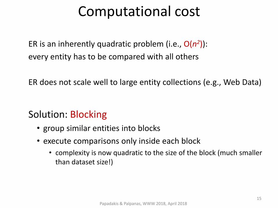
Computational cost
ER is an inherently quadratic problem (i.e., O(n2)):
every entity has to be compared with all others
ER does not scale well to large entity collections (e.g., Web Data)
Solution: Blocking • group similar entities into blocks
• execute comparisons only inside each block
• complexity is now quadratic to the size of the block (much smaller than dataset size!)
Papadakis & Palpanas, WWW 2018, April 2018 15

Computational cost
|E| entities
|E| entities
Brute-force approach
Duplicate Pairs
Blocking Input: Entity Collection E
Papadakis & Palpanas, WWW 2018, April 2018 16

Example of Computational cost
DBPedia 3.0rc ↔ DBPedia 3.4 1.2 million entities ↔ 2.2 million entities
Entity matching: Jaccard similarity of all tokens Cost per comparison: 0.045 milliseconds (average of 0.1 billion comparisons)
Brute-force approach Comparisons: 2.58 ∙ 1012
Recall: 100% Running time: 1,344 days → 3.7 years
Optimized Token Blocking Workflow Overhead time: 4 hours Comparisons: 8.95 ∙ 106 Recall: 99% Total Running time: 10 hours
Papadakis & Palpanas, WWW 2018, April 2018 17

Example of Computational cost
DBPedia 3.0rc ↔ DBPedia 3.4 1.2 million entities ↔ 2.2 million entities
Entity matching: Jaccard similarity of all tokens Cost per comparison: 0.045 milliseconds (average of 0.1 billion comparisons)
Brute-force approach Comparisons: 2.58 ∙ 1012
Recall: 100% Running time: 1,344 days → 3.7 years
Optimized Token Blocking Workflow Overhead time: 4 hours Comparisons: 8.95 ∙ 106 Recall: 99% Total Running time: 10 hours
Papadakis & Palpanas, WWW 2018, April 2018 18

Scalable End-to-end ER workflow
Block Building
Block Processing
Entity Matching
Entity Clustering
Step 3 Step 1 Step 2 Step 4
Cluster together similar entities
Refine blocks to increase precision at
no significant cost in recall
Compare the candidate matches
Partition the compared
profiles into real-world
entities
Papadakis & Palpanas, WWW 2018, April 2018 19

Outline
1. Introduction to Blocking 2. Blocking Methods for Relational Data 3. Blocking Methods for Web Data 4. Block Processing Techniques 5. Meta-blocking 6. Entity Matching 7. Entity Clustering 8. Massive Parallelization Methods 9. Progressive Entity Resolution 10.Challenges 11.JedAI Toolkit 12.Conclusions
Papadakis & Palpanas, WWW 2018, April 2018 20

Papadakis & Palpanas, WWW 2018, April 2018
Part 1:
Introduction to Blocking
21

Fundamental Assumptions
1. Every entity profile consists of a uniquely identified set of name-value pairs.
2. Every entity profile corresponds to a single real-world object.
3. Two matching profiles are detected as long as they co-occur in at least one block → entity matching is an orthogonal problem.
4. Focus on string values.
Papadakis & Palpanas, WWW 2018, April 2018 22

General Principles
1. Represent each entity by one or more blocking keys.
2. Place into blocks all entities having the same or similar blocking key.
Measures for assessing block quality [Christen, TKDE 2011]:
– Pairs Completeness: 𝑃𝐶 =𝑑𝑒𝑡𝑒𝑐𝑡𝑒𝑑 𝑚𝑎𝑡𝑐ℎ𝑒𝑠
𝑒𝑥𝑖𝑠𝑡𝑖𝑛𝑔 𝑚𝑎𝑡𝑐ℎ𝑒𝑠 (optimistic recall)
– Pairs Quality: 𝑃𝑄 =𝑑𝑒𝑡𝑒𝑐𝑡𝑒𝑑 𝑚𝑎𝑡𝑐ℎ𝑒𝑠
𝑒𝑥𝑒𝑐𝑢𝑡𝑒𝑑 𝑐𝑜𝑚𝑝𝑎𝑟𝑖𝑠𝑜𝑛𝑠 (pessimistic precision)
Trade-off!
Papadakis & Palpanas, WWW 2018, April 2018
23

Problem Definition
Given one dirty (Dirty ER), or two clean (Clean-Clean ER)
entity collections, cluster their profiles into blocks
and process them so that both Pairs Completeness (PC) and Pairs Quality (PQ) are maximized.
caution:
• Emphasis on Pairs Completeness (PC). – if two entities are matching then they should coincide at some block
Papadakis & Palpanas, WWW 2018, April 2018 24

Blocking Techniques Taxonomy
1. Performance-wise • Exact methods
• Approximate methods
2. Functionality-wise • Supervised methods
• Unsupervised methods
3. Blocks-wise • Disjoint blocks
• Overlapping blocks
– Redundancy-neutral
– Redundancy-positive
– Redundancy-negative
4. Signature-wise • Schema-based
• Schema-agnostic
Papadakis & Palpanas, WWW 2018, April 2018 25
Papadakis & Palpanas, WWW 2018, April 2018
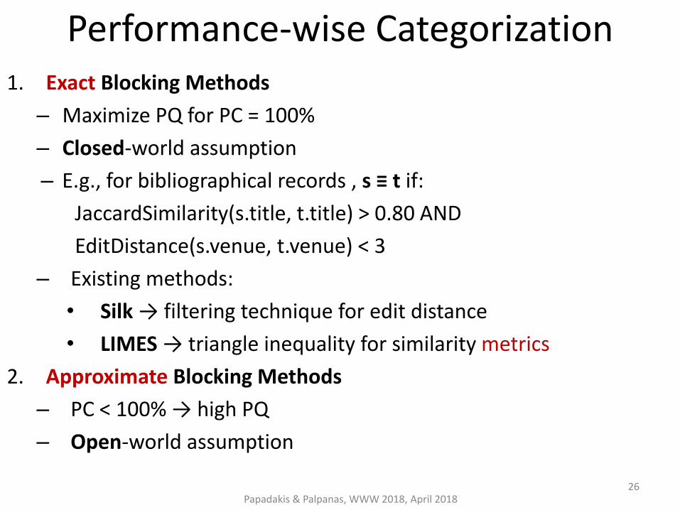
Performance-wise Categorization 1. Exact Blocking Methods
– Maximize PQ for PC = 100%
– Closed-world assumption
– E.g., for bibliographical records , s ≡ t if:
JaccardSimilarity(s.title, t.title) > 0.80 AND
EditDistance(s.venue, t.venue) < 3
– Existing methods:
• Silk → filtering technique for edit distance
• LIMES → triangle inequality for similarity metrics
2. Approximate Blocking Methods
– PC < 100% → high PQ
– Open-world assumption
26
Papadakis & Palpanas, WWW 2018, April 2018
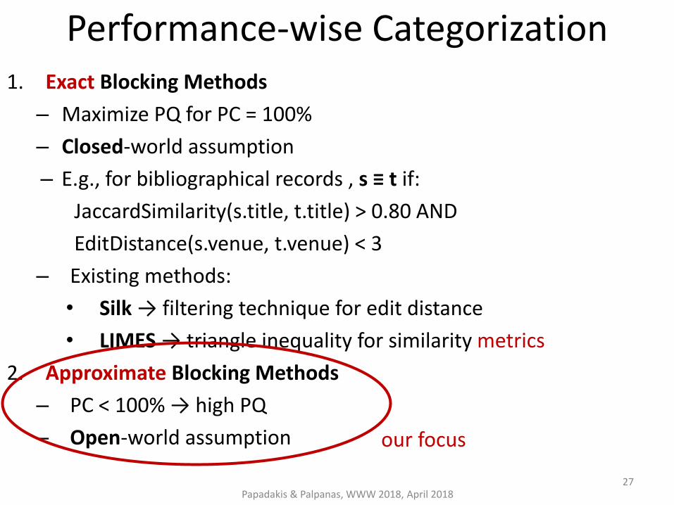
Performance-wise Categorization 1. Exact Blocking Methods
– Maximize PQ for PC = 100%
– Closed-world assumption
– E.g., for bibliographical records , s ≡ t if:
JaccardSimilarity(s.title, t.title) > 0.80 AND
EditDistance(s.venue, t.venue) < 3
– Existing methods:
• Silk → filtering technique for edit distance
• LIMES → triangle inequality for similarity metrics
2. Approximate Blocking Methods
– PC < 100% → high PQ
– Open-world assumption our focus
27

Papadakis & Palpanas, WWW 2018, April 2018
Functionality-wise Categorization 1. Supervised Methods
• Goal: learn the best blocking keys from a training set
• Approach: identify best combination of attribute names and transformations
• E.g., CBLOCK [Sarma et. al, CIKM 2012],
[Bilenko et. al., ICDM 2006], [Michelson et. al., AAAI 2006]
• Drawbacks: – labelled data
– domain-dependent
2. Unsupervised Methods
• Generic, popular methods
28

Papadakis & Palpanas, WWW 2018, April 2018
Functionality-wise Categorization 1. Supervised Methods
• Goal: learn the best blocking keys from a training set
• Approach: identify best combination of attribute names and transformations
• E.g., CBLOCK [Sarma et. al, CIKM 2012],
[Bilenko et. al., ICDM 2006], [Michelson et. al., AAAI 2006]
• Drawbacks: – labelled data
– domain-dependent
2. Unsupervised Methods
• Generic, popular methods our focus
29
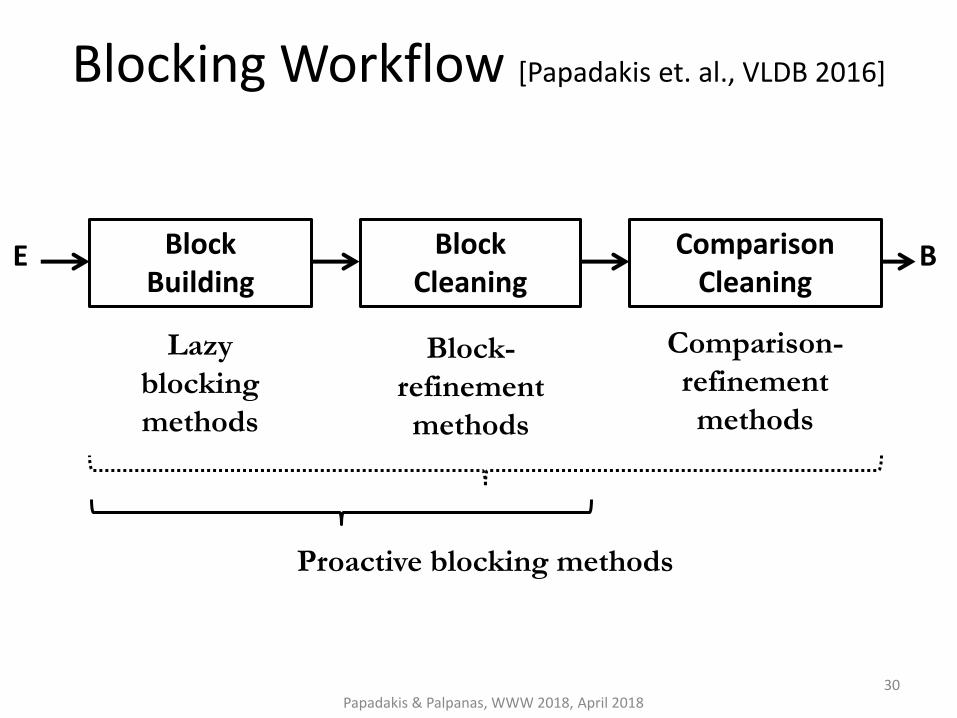
Block Building
Comparison Cleaning
E B Block Cleaning
Lazy
blocking
methods
Block-
refinement
methods
Comparison-
refinement
methods
Proactive blocking methods
Blocking Workflow [Papadakis et. al., VLDB 2016]
Papadakis & Palpanas, WWW 2018, April 2018 30

Blocks- and Signature-wise Categorization of Block Building Methods
Papadakis & Palpanas, WWW 2018, April 2018
Disjoint Blocks
Overlapping Blocks
Redundancy- negative
Redundancy- neutral
Redundancy- positive
Schema- based
Standard Blocking
(Extended) Canopy
Clustering
1. (Extended) Sorted Neighborhood
2. MFIBlocks
1. (Extended) Q-grams Blocking 2. (Extended) Suffix Arrays
Schema- agnostic
- - -
1. Token Blocking 2. Agnostic Clustering 3. TYPiMatch 4. URI Semantics Blocking
31

Papadakis & Palpanas, WWW 2018, April 2018
Block Processing Methods [Papadakis et. al., VLDB 2016]
Mostly for redundancy-positive block building methods.
Block Cleaning
• Block-level – constraints on block characteristics
• Entity-level – constraints on entity characteristics
Comparison Cleaning
• Redundant comparisons – repeated across different blocks
• Superfluous comparisons – Involve non-matching entities
32

Papadakis & Palpanas, WWW 2018, April 2018
Part 2:
Block Building for Relational Data
33

General Principles
Mostly schema-based techniques.
Rely on two assumptions:
1. A-priori known schema → no noise in attribute names.
2. For each attribute name we know some metadata:
– level of noise (e.g., spelling mistakes, false or missing values)
– distinctiveness of values
Papadakis & Palpanas, WWW 2018, April 2018 34

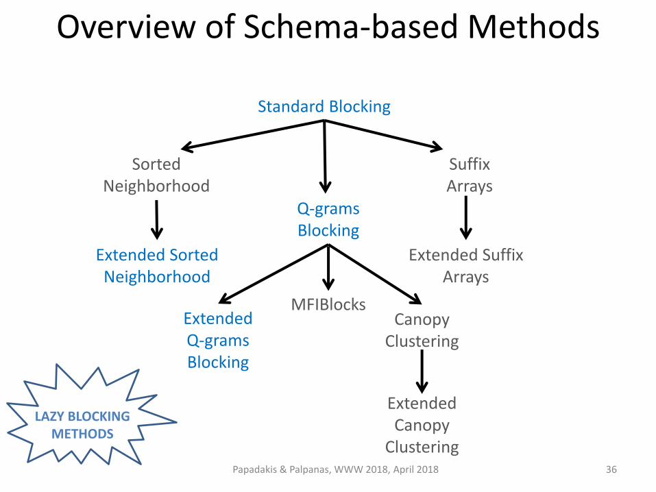
Standard Blocking
Sorted Neighborhood
Extended Sorted Neighborhood
Q-grams Blocking
Extended Q-grams Blocking
Suffix Arrays
Canopy Clustering
Extended Canopy
Clustering
Overview of Schema-based Methods
Papadakis & Palpanas, WWW 2018, April 2018
MFIBlocks
Extended Suffix Arrays
35
Standard Blocking
Sorted Neighborhood
Extended Sorted Neighborhood
Q-grams Blocking
Extended Q-grams Blocking
Suffix Arrays
Canopy Clustering
Extended Canopy
Clustering
Overview of Schema-based Methods
Papadakis & Palpanas, WWW 2018, April 2018
MFIBlocks
Extended Suffix Arrays
LAZY BLOCKING METHODS
36

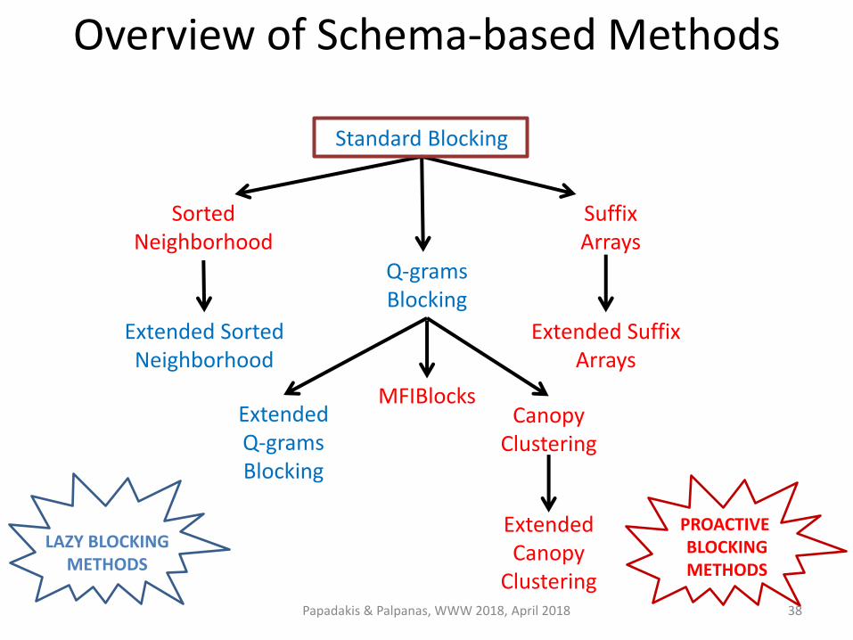
Standard Blocking
Sorted Neighborhood
Extended Sorted Neighborhood
Q-grams Blocking
Extended Q-grams Blocking
Suffix Arrays
Canopy Clustering
Extended Canopy
Clustering
Overview of Schema-based Methods
Papadakis & Palpanas, WWW 2018, April 2018
MFIBlocks
Extended Suffix Arrays
LAZY BLOCKING METHODS
PROACTIVE BLOCKING METHODS
37
Standard Blocking
Sorted Neighborhood
Extended Sorted Neighborhood
Q-grams Blocking
Extended Q-grams Blocking
Suffix Arrays
Canopy Clustering
Extended Canopy
Clustering
Overview of Schema-based Methods
Papadakis & Palpanas, WWW 2018, April 2018
MFIBlocks
Extended Suffix Arrays
LAZY BLOCKING METHODS
PROACTIVE BLOCKING METHODS
38
Standard Blocking [Fellegi et. al., JASS 1969]
Earliest, simplest form of blocking.
Algorithm:
1. Select the most appropriate attribute name(s) w.r.t. noise and distinctiveness.
2. Transform the corresponding value(s) into a Blocking Key (BK)
3. For each BK, create one block that contains all entities having this BK in their transformation.
Works as a hash function! → Blocks on the equality of BKs
Papadakis & Palpanas, WWW 2018, April 2018 39

Example of Standard Blocking
Papadakis & Palpanas, WWW 2018, April 2018
Blocks on zip_code:
40

Standard Blocking
Sorted Neighborhood
Extended Sorted Neighborhood
Q-grams Blocking
Extended Q-grams Blocking
Suffix Arrays
Canopy Clustering
Extended Canopy
Clustering
Overview of Schema-based Methods
Papadakis & Palpanas, WWW 2018, April 2018
MFIBlocks
Extended Suffix Arrays
41

Standard Blocking
Sorted Neighborhood
Extended Sorted Neighborhood
Q-grams Blocking
Extended Q-grams Blocking
Suffix Arrays
Canopy Clustering
Extended Canopy
Clustering
Overview of Schema-based Methods blocks contain entities with similar blocking keys
Papadakis & Palpanas, WWW 2018, April 2018
MFIBlocks
Extended Suffix Arrays
42
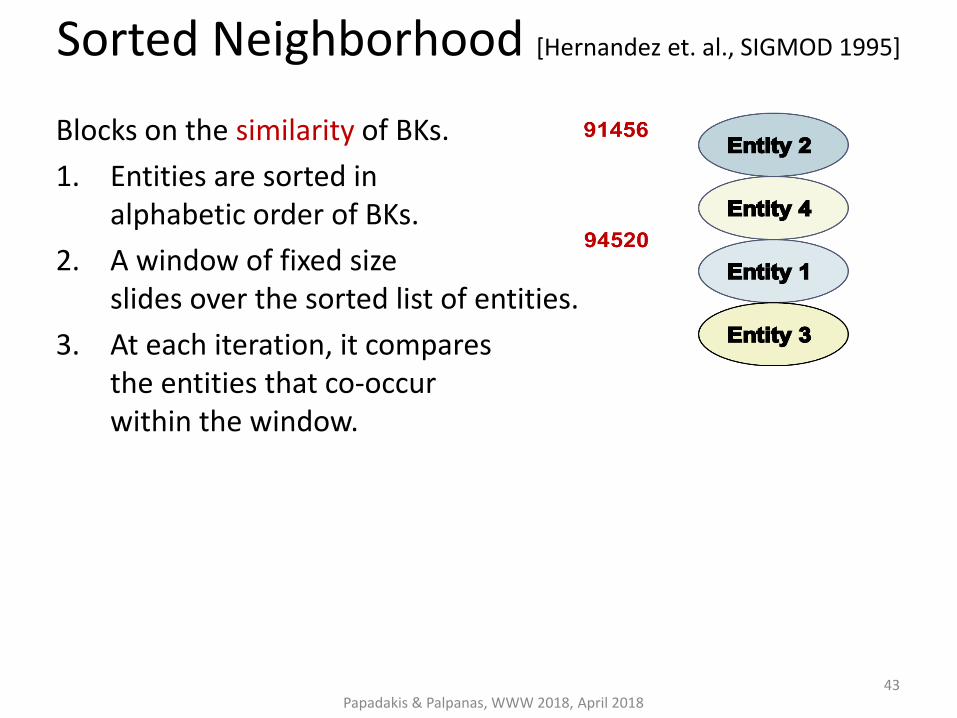
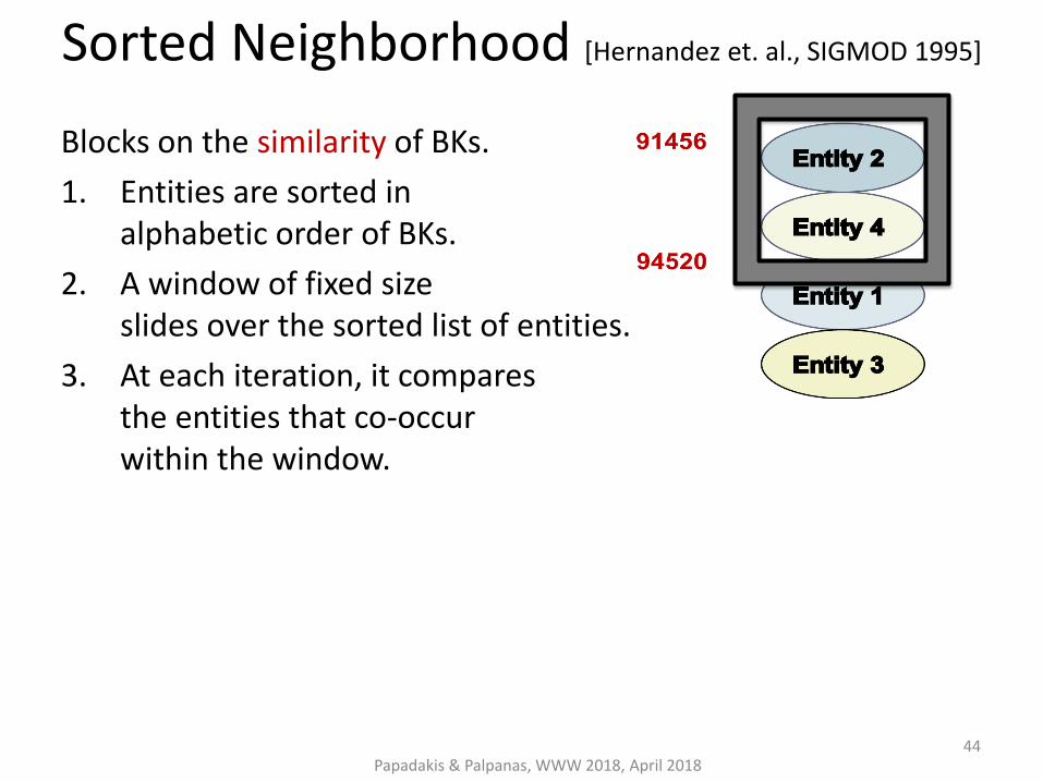
Sorted Neighborhood [Hernandez et. al., SIGMOD 1995]
Blocks on the similarity of BKs.
1. Entities are sorted in alphabetic order of BKs.
2. A window of fixed size slides over the sorted list of entities.
3. At each iteration, it compares the entities that co-occur within the window.
Papadakis & Palpanas, WWW 2018, April 2018 43
Sorted Neighborhood [Hernandez et. al., SIGMOD 1995]
Blocks on the similarity of BKs.
1. Entities are sorted in alphabetic order of BKs.
2. A window of fixed size slides over the sorted list of entities.
3. At each iteration, it compares the entities that co-occur within the window.
Papadakis & Palpanas, WWW 2018, April 2018 44

Sorted Neighborhood [Hernandez et. al., SIGMOD 1995]
Blocks on the similarity of BKs.
1. Entities are sorted in alphabetic order of BKs.
2. A window of fixed size slides over the sorted list of entities.
3. At each iteration, it compares the entities that co-occur within the window.
Papadakis & Palpanas, WWW 2018, April 2018 45

Sorted Neighborhood [Hernandez et. al., SIGMOD 1995]
Blocks on the similarity of BKs.
1. Entities are sorted in alphabetic order of BKs.
2. A window of fixed size slides over the sorted list of entities.
3. At each iteration, it compares the entities that co-occur within the window.
Papadakis & Palpanas, WWW 2018, April 2018 46

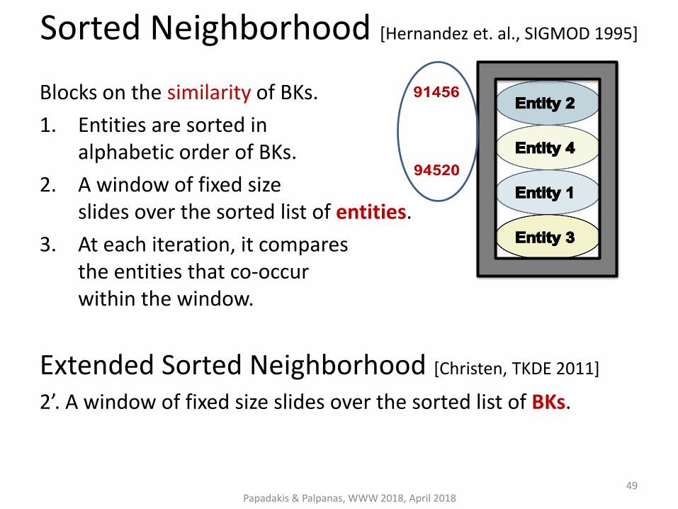
Sorted Neighborhood [Hernandez et. al., SIGMOD 1995]
Blocks on the similarity of BKs.
1. Entities are sorted in alphabetic order of BKs.
2. A window of fixed size slides over the sorted list of entities.
3. At each iteration, it compares the entities that co-occur within the window.
Extended Sorted Neighborhood [Christen, TKDE 2011]
2’. A window of fixed size slides over the sorted list of BKs.
Papadakis & Palpanas, WWW 2018, April 2018 47

Sorted Neighborhood [Hernandez et. al., SIGMOD 1995]
Blocks on the similarity of BKs.
1. Entities are sorted in alphabetic order of BKs.
2. A window of fixed size slides over the sorted list of entities.
3. At each iteration, it compares the entities that co-occur within the window.
Extended Sorted Neighborhood [Christen, TKDE 2011]
2’. A window of fixed size slides over the sorted list of BKs.
Papadakis & Palpanas, WWW 2018, April 2018 48
Sorted Neighborhood [Hernandez et. al., SIGMOD 1995]
Blocks on the similarity of BKs.
1. Entities are sorted in alphabetic order of BKs.
2. A window of fixed size slides over the sorted list of entities.
3. At each iteration, it compares the entities that co-occur within the window.
Extended Sorted Neighborhood [Christen, TKDE 2011]
2’. A window of fixed size slides over the sorted list of BKs.
Papadakis & Palpanas, WWW 2018, April 2018 49

Standard Blocking
Sorted Neighborhood
Extended Sorted Neighborhood
Q-grams Blocking
Extended Q-grams Blocking
Suffix Arrays
Canopy Clustering
Extended Canopy
Clustering
Overview of Schema-based Methods
Papadakis & Palpanas, WWW 2018, April 2018
MFIBlocks
Extended Suffix Arrays
50

Standard Blocking
Sorted Neighborhood
Extended Sorted Neighborhood
Q-grams Blocking
Extended Q-grams Blocking
Suffix Arrays
Canopy Clustering
Extended Canopy
Clustering
Overview of Schema-based Methods blocks contain entities with same, or similar blocking keys
Papadakis & Palpanas, WWW 2018, April 2018
MFIBlocks
Extended Suffix Arrays
51

Q-grams Blocking [Gravano et. al., VLDB 2001]
Blocks on equality of BKs.
Converts every BK into the list of its q-grams.
For q=2, the BKs 91456 and 94520 yield the following blocks:
• Advantage:
robust to noisy BKVs
• Drawback:
larger blocks → higher computational cost
Papadakis & Palpanas, WWW 2018, April 2018 52

Extended Q-grams Blocking [Baxter et. al., KDD 2003]
BKs of higher discriminativeness: instead of individual q-grams, BKs from combinations of q-grams.
Additional parameter: threshold t ∈ (0,1) specifies the minimum number of q-grams per BK as follows: 𝒍𝒎𝒊𝒏 = 𝒎𝒂𝒙(𝟏, 𝐤 ∙ 𝒕 ), where 𝑘 is the number of q-grams from the original BK
Example: for BK= 91456, q=2 and t=0.9, we have lmin=3 and the following valid BKs: 91_14_45_56 91_14_45 91_14_56 91_45_56 14_45_56
Papadakis & Palpanas, WWW 2018, April 2018 53

MFIBlocks [Kenig et. al., IS 2013]
Papadakis & Palpanas, WWW 2018, April 2018
Based on mining Maximum Frequent Itemsets. Algorithm: • Place all entities in a pool • while (minimum_support > 2)
– For each itemset that satisfies minimum_support • Create a block b • If b satisfies certain constraints (Block Cleaning)
– remove its entities from the pool – retain the best comparisons (Comparison Cleaning)
– decrease minimum_support
Pros: • Usually the most effective blocking method for relational data →
maximizes PQ (precision)
Cons: • Difficult to configure • Time consuming 54

Standard Blocking
Sorted Neighborhood
Extended Sorted Neighborhood
Q-grams Blocking
Extended Q-grams Blocking
Suffix Arrays
Canopy Clustering
Extended Canopy
Clustering
Overview of Schema-based Methods
Papadakis & Palpanas, WWW 2018, April 2018
MFIBlocks
Extended Suffix Arrays
55

Standard Blocking
Sorted Neighborhood
Extended Sorted Neighborhood
Q-grams Blocking
Extended Q-grams Blocking
Suffix Arrays
Canopy Clustering
Extended Canopy
Clustering Papadakis & Palpanas, WWW 2018, April 2018
MFIBlocks
Extended Suffix Arrays
Overview of Schema-based Methods blocks contain entities with similar blocking keys
56

Canopy Clustering [McCallum et. al., KDD 2000]
Papadakis & Palpanas, WWW 2018, April 2018
Blocks on similarity of BKs.
57

Extended Canopy Clustering [Christen, TKDE 2011]
Canopy Clustering is too sensitive w.r.t. its weight thresholds:
- high values may leave many entities out of blocks.
Solution: Extended Canopy Clustering [Christen, TKDE 2011]
• cardinality thresholds instead of weight thresholds
• for each center of a canopy:
– the n1 nearest entities are placed in its block
– the n2 (≤ n1) nearest entities are removed from the pool
Papadakis & Palpanas, WWW 2018, April 2018 58

Standard Blocking
Sorted Neighborhood
Extended Sorted Neighborhood
Q-grams Blocking
Extended Q-grams Blocking
Suffix Arrays
Canopy Clustering
Extended Canopy
Clustering
Overview of Schema-based Methods
Papadakis & Palpanas, WWW 2018, April 2018
MFIBlocks
Extended Suffix Arrays
59

Standard Blocking
Sorted Neighborhood
Extended Sorted Neighborhood
Q-grams Blocking
Extended Q-grams Blocking
Suffix Arrays
Canopy Clustering
Extended Canopy
Clustering Papadakis & Palpanas, WWW 2018, April 2018
MFIBlocks
Extended Suffix Arrays
Overview of Schema-based Methods blocks contain entities with same blocking keys
60

Suffix Arrays Blocking [Aizawa et. al., WIRI 2005]
Blocks on the equality of BKs.
Converts every BK to the list of its suffixes that are longer than a predetermined minimum length lmin.
For lmin =3, the keys 91456 and 94520 yield the blocks:
Frequent suffixes are discarded with the help of the parameter bM:
- specifies the maximum number of entities per block
Papadakis & Palpanas, WWW 2018, April 2018 62

Extended Suffix Arrays Blocking [Christen, TKDE 2011]
Goal:
support errors at the end of BKs
Solution:
consider all substrings (not only suffixes) with more than lmin
characters.
For lmin=3, the keys 91456 and 94520 are converted to the BKs:
91456, 94520
9145, 9452
1456, 4520
914, 945
145, 452
456 520
Papadakis & Palpanas, WWW 2018, April 2018
63
Summary of Blocking for Databases [Christen, TKDE2011]
1. They typically employ redundancy to ensure higher recall in the context of noise at the cost of lower precision (more comparisons). Still, recall remains low for many datasets.
2. Several parameters to be configured
E.g., Canopy Clustering has the following parameters:
I. String matching method
II. Threshold t1
III. Threshold t2
3. Schema-dependent → manual definition of BKs
Papadakis & Palpanas, WWW 2018, April 2018 64

Improving Blocking for Databases [Papadakis et. al., VLDB 2015]
Schema-agnostic blocking keys
• Use every token as a key
• Applies to all schema-based blocking methods
• Simplifies configuration, unsupervised approach
Performance evaluation
• For lazy blocking methods → very high, robust recall at the cost of more comparisons
• For proactive blocking methods → relative recall gets higher with more comparisons, absolute recall depends on block constraints
Papadakis & Palpanas, WWW 2018, April 2018 65

Papadakis & Palpanas, WWW 2018, April 2018
Part 3:
Block Building for Web Data
66

Characteristics of Web Data
Voluminous, (semi-)structured datasets.
• DBPedia 2014: 3 billion triples and 38 million entities
• BTC09: 1.15 billion triples, 182 million entities.
Users are free to add attribute values and/or attribute names
unprecedented levels of schema heterogeneity.
• DBPedia 3.4: 50,000 attribute names
• Google Base: 100,000 schemata for 10,000 entity types
• BTC09: 136,000 attribute names
Several datasets produced by automatic information extraction techniques
noise, tag-style values.
Papadakis & Palpanas, WWW 2018, April 2018
67
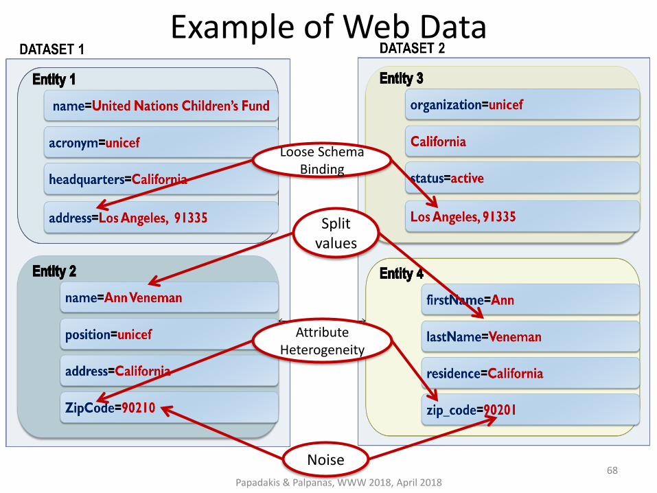
Example of Web Data
Noise
Attribute Heterogeneity
Loose Schema Binding
Split values
Papadakis & Palpanas, WWW 2018, April 2018 68

Token Blocking [Papadakis et al., WSDM2011]
Functionality:
1. given an entity profile, extract all tokens that are contained in its attribute values.
2. create one block for every distinct token → each block contains all entities with the corresponding token*.
Attribute-agnostic functionality:
• completely ignores all attribute names, but considers all attribute values
• efficient implementation with the help of inverted indices
• parameter-free!
*Each block should contain at least two entities.
Papadakis & Palpanas, WWW 2018, April 2018 69

Token Blocking Example
Papadakis & Palpanas, WWW 2018, April 2018 70

Attribute-Clustering Blocking [Papadakis et. al., TKDE 2013]
Goal:
group attribute names into clusters s.t. we can apply Token Blocking independently inside each cluster, without affecting effectiveness → smaller blocks, higher efficiency.
Papadakis & Palpanas, WWW 2018, April 2018
Building address
headquarters hdq
Person address
address residence
71

Attribute-Clustering Blocking Algorithm
• Create a graph, where every node represents an attribute name and its attribute values
• For each attribute name/node ni
– Find the most similar node nj
– If sim(ni,nj) > 0, add an edge <ni,nj> • Extract connected components • Put all singleton nodes in a “glue” cluster
Parameters
1. Representation model
– Character n-grams, Character n-gram graphs, Tokens
2. Similarity Metric
– Jaccard, Graph Value Similarity, TF-IDF
Papadakis & Palpanas, WWW 2018, April 2018 72

Attribute-Clustering vs Schema Matching
Similar to Schema Matching, …but fundamentally different:
1. Associated attribute names do not have to be semantically equivalent. They only have to produce good blocks
2. All singleton attribute names are associated with each other
3. Unlike Schema Matching, it scales to the very high levels of heterogeneity of Web Data – because of the above simplifying assumptions
Papadakis & Palpanas, WWW 2018, April 2018 73

TYPiMatch [Ma et. al., WSDM 2013]
Goal:
cluster entities into overlapping types and apply Token
Blocking to the values of the best attribute for each type.
Papadakis & Palpanas, WWW 2018, April 2018
persons
organizations
74

TYPiMatch
Algorithm:
1. Create a directed graph G, where nodes correspond to tokens, and edges connect those co-occurring in the same entity profile, weighted according to conditional co-occurrence probability.
2. Convert G to undirected graph G’ and get maximal cliques (parameter θ).
3. Create an undirected graph G’’, where nodes correspond to cliques and edges connect the frequently co-occurring cliques (parameter ε).
4. Get connected components to form entity types.
5. Get best attribute name for each type using an entropy-based criterion.
Papadakis & Palpanas, WWW 2018, April 2018 75

For Semantic Web data, three sources of evidence create blocks of lower redundancy than Token Blocking:
1.Infix
2. Infix Profile
3.Literal Profile
Algorithm for URI decomposition in PI(S)-form in [Papadakis et al., iiWAS 2010].
Evidence for Semantic Web Blocking
Papadakis & Palpanas, WWW 2018, April 2018 76

The above sources of evidence lead to 3 parameter-free blocking methods:
1. Infix Blocking every block contains all entities whose URI has a specific Infix
2. Infix Profile Blocking every block corresponds to a specific Infix (of an attribute value) and contains all entities having it in their Infix Profile
3. Literal Profile Blocking every block corresponds to a specific token and contains all entities having it in their Literal Profile
Individually, these atomic methods have limited coverage and,
thus, low effectiveness (e.g., Infix Blocking does not cover blank
nodes).
However, they are complementary and can be combined
into composite blocking methods with high robustness and
effectiveness!
URI Semantics Blocking [Papadakis et al., WSDM2012]
Papadakis & Palpanas, WWW 2018, April 2018 77

Summary of Blocking for Web Data
High Recall in the context of noisy entity profiles and extreme schema heterogeneity thanks to:
1. redundancy that reduces the likelihood of missed matches.
2. attribute-agnostic functionality that requires no schema semantics.
Low Precision because:
• the blocks are overlapping → redundant comparisons
• high number of comparisons between irrelevant entities → superfluous comparisons
Papadakis & Palpanas, WWW 2018, April 2018 78

Token Blocking Example
Papadakis & Palpanas, WWW 2018, April 2018
Superfluous Comparison
Redundant Comparison
79
Papadakis & Palpanas, WWW 2018, April 2018
Part 4:
Block Processing Techniques
80

Outline 1. Introduction to Blocking 2. Blocking Methods for Relational Data 3. Blocking Methods for Web Data
4. Block Processing Techniques – Block Purging – Block Filtering – Block Clustering – Comparison Propagation – Iterative Blocking
5. Meta-blocking 6. Entity Matching 7. Entity Clustering 8. Massive Parallelization Methods 9. Progressive Entity Resolution 10. Challenges 11. JedAI Toolkit 12. Conclusions
Papadakis & Palpanas, WWW 2018, April 2018 81

General Principles
Goals:
1. eliminate all redundant comparisons
2. avoid most superfluous comparisons
without affecting matching comparisons (i.e., PC).
Depending on the granularity of their functionality, they are distinguished into:
1. Block-refinement
2. Comparison-refinement
• Iterative Methods
Papadakis & Palpanas, WWW 2018, April 2018 82

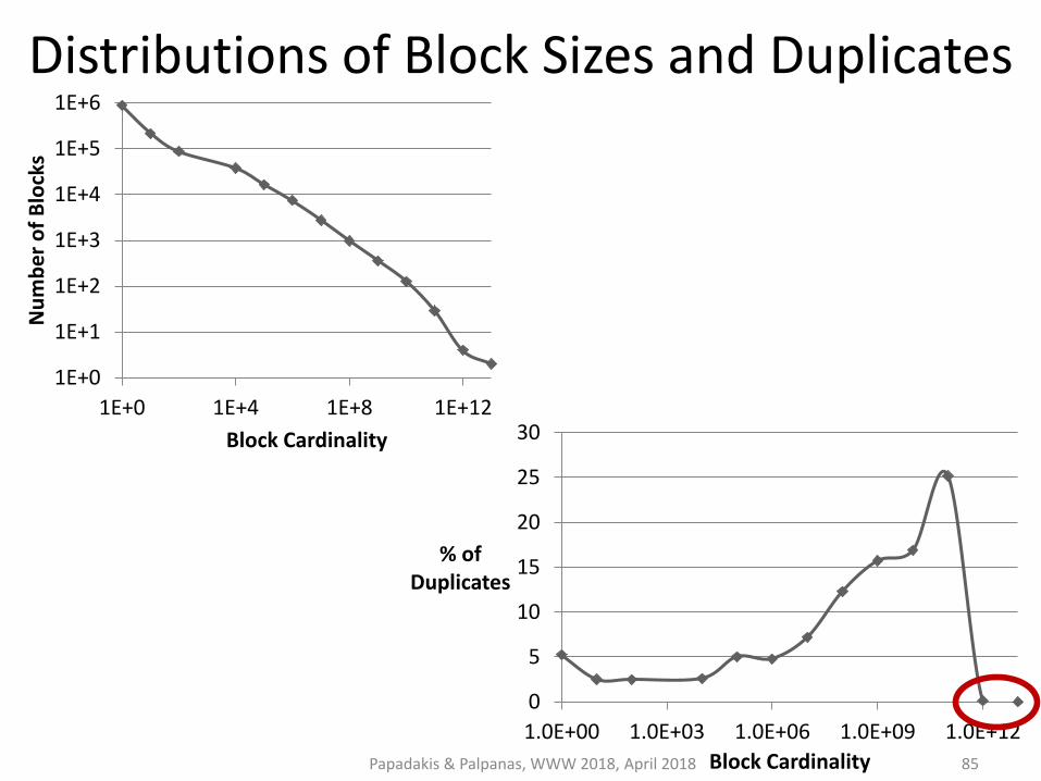
Block Purging
Exploits power-law distribution of block sizes.
Targets oversized blocks (i.e., many comparisons, no duplicates)
Discards them by setting an upper limit on:
• the size of each block [Papadakis et al., WSDM 2011],
• the cardinality of each block [Papadakis et al., WSDM 2012]
Core method:
• Low computational cost.
• Low impact on effectiveness.
• Boosts efficiency to a large extent. Papadakis & Palpanas, WWW 2018, April 2018
83

Distributions of Block Sizes and Duplicates
Papadakis & Palpanas, WWW 2018, April 2018
1E+0
1E+1
1E+2
1E+3
1E+4
1E+5
1E+6
1E+0 1E+4 1E+8 1E+12
Nu
mb
er o
f B
lock
s
Block Cardinality
84
0
5
10
15
20
25
30
1.0E+00 1.0E+03 1.0E+06 1.0E+09 1.0E+12
% of Duplicates
Block Cardinality
Distributions of Block Sizes and Duplicates
0
5
10
15
20
25
30
1.0E+00 1.0E+03 1.0E+06 1.0E+09 1.0E+12
% of Duplicates
Block Cardinality Papadakis & Palpanas, WWW 2018, April 2018
1E+0
1E+1
1E+2
1E+3
1E+4
1E+5
1E+6
1E+0 1E+4 1E+8 1E+12
Nu
mb
er o
f B
lock
s
Block Cardinality
85

1E+0
1E+1
1E+2
1E+3
1E+4
1E+5
1E+6
1E+0 1E+4 1E+8 1E+12
Nu
mb
er o
f B
lock
s
Block Cardinality
Distributions of Block Sizes and Duplicates
0
5
10
15
20
25
30
1.0E+00 1.0E+03 1.0E+06 1.0E+09 1.0E+12
% of Duplicates
Block Cardinality Papadakis & Palpanas, WWW 2018, April 2018 86

Block Filtering [Papadakis et. al, EDBT 2016]
Main ideas:
• each block has a different importance for every entity it contains.
• Larger blocks are less likely to contain unique duplicates and, thus, are less important.
Algorithm
• sort blocks in ascending cardinality
• build Entity Index
• retain every entity in r% of its smallest blocks
• reconstruct blocks
Papadakis & Palpanas, WWW 2018, April 2018 87

Block Filtering Example
Papadakis & Palpanas, WWW 2018, April 2018 88

Block Clustering [Fisher et. al., KDD 2015]
Main idea:
• restrict the size of every block into [bmin, bmax]
– necessary in applications like privacy-preserving ER
– operates so that ||B|| increases linearly with |E|
Algorithm
• recursive agglomerative clustering
– merge similar blocks with size lower than bmin
– split blocks with size larger than bmax
• until all blocks have the desired size
Papadakis & Palpanas, WWW 2018, April 2018 89

Comparison Propagation [Papadakis et al., JCDL 2011]
• Eliminate all redundant comparisons at no cost in recall.
• Naïve approach does not scale.
• Functionality:
1. Build Entity Index
2. Least Common Block Index condition.
Papadakis & Palpanas, WWW 2018, April 2018
90

Iterative Blocking [Whang et. Al, SIGMOD 2009]
Main idea:
integrate block processing with entity matching and reflect outcomes to subsequently processed blocks, until no new matches are detected.
Algorithm
• Put all blocks in a queue Q
• While Q is not empty
– Get first block
– Get matches with an ER algorithm (e.g., R-Swoosh)
• For each new pair of duplicates pi≡pj
– Merge their profiles p’i = p’j =< pi, pj > and update them in all associated blocks
– Place in Q all associated blocks that are not already in it
Papadakis & Palpanas, WWW 2018, April 2018 91

Papadakis & Palpanas, WWW 2018, April 2018
Part 5:
Meta-blocking
92

Motivation
DBPedia 3.0rc ↔ DBPedia 3.4
1.2 million entities ↔ 2.2 million entities
Papadakis & Palpanas, WWW 2018, April 2018
Block Building
Comparison Cleaning
E B Block Cleaning
93

Motivation
DBPedia 3.0rc ↔ DBPedia 3.4
1.2 million entities ↔ 2.2 million entities
Brute-force approach
Comparisons: 2.58 ∙ 1012
Recall: 100%
Running time: 1,344 days → 3.7 years
Papadakis & Palpanas, WWW 2018, April 2018
Block Building
Comparison Cleaning
E B Block Cleaning
94
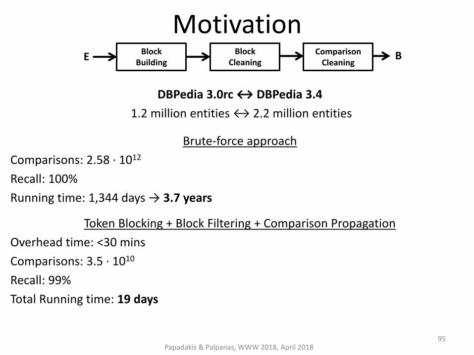
Motivation
DBPedia 3.0rc ↔ DBPedia 3.4
1.2 million entities ↔ 2.2 million entities
Brute-force approach
Comparisons: 2.58 ∙ 1012
Recall: 100%
Running time: 1,344 days → 3.7 years
Token Blocking + Block Filtering + Comparison Propagation
Overhead time: <30 mins
Comparisons: 3.5 ∙ 1010
Recall: 99%
Total Running time: 19 days
Papadakis & Palpanas, WWW 2018, April 2018
Block Building
Comparison Cleaning
E B Block Cleaning
95

Motivation
DBPedia 3.0rc ↔ DBPedia 3.4
1.2 million entities ↔ 2.2 million entities
Brute-force approach
Comparisons: 2.58 ∙ 1012
Recall: 100%
Running time: 1,344 days → 3.7 years
Token Blocking + Block Filtering + Comparison Propagation
Overhead time: <30 mins
Comparisons: 3.5 ∙ 1010
Recall: 99%
Total Running time: 19 days
Papadakis & Palpanas, WWW 2018, April 2018
Block Building
Comparison Cleaning
E B Block Cleaning
96

Motivation
DBPedia 3.0rc ↔ DBPedia 3.4
1.2 million entities ↔ 2.2 million entities
Brute-force approach
Comparisons: 2.58 ∙ 1012
Recall: 100%
Running time: 1,344 days → 3.7 years
Token Blocking + Block Filtering + Comparison Propagation
Overhead time: <30 mins
Comparisons: 3.5 ∙ 1010
Recall: 99%
Total Running time: 19 days
Token Blocking + Block Filtering + ??
Papadakis & Palpanas, WWW 2018, April 2018
Block Building
Comparison Cleaning
E B Block Cleaning
97
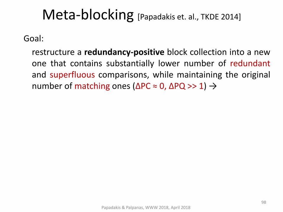
Meta-blocking [Papadakis et. al., TKDE 2014]
Goal:
restructure a redundancy-positive block collection into a new one that contains substantially lower number of redundant and superfluous comparisons, while maintaining the original number of matching ones (ΔPC ≈ 0, ΔPQ >> 1) →
Papadakis & Palpanas, WWW 2018, April 2018 98

Meta-blocking [Papadakis et. al., TKDE 2014]
Goal:
restructure a redundancy-positive block collection into a new one that contains substantially lower number of redundant and superfluous comparisons, while maintaining the original number of matching ones (ΔPC ≈ 0, ΔPQ >> 1) →
Main idea:
common blocks provide valuable evidence for the similarity of entities
→ the more blocks two entities share, the more similar and the more likely they are to be matching
Papadakis & Palpanas, WWW 2018, April 2018
99

Outline of Meta-blocking
n1 n3
n2 n4
n1 n3
n2 n4
n1 n3
n2 n4
3
3
2 2 2
1
Papadakis & Palpanas, WWW 2018, April 2018 100

Graph Building
For every block:
• for every entity → add a node
• for every pair of co-occurring entities → add an undirected edge
Blocking graph:
• It eliminates all redundant comparisons → no parallel edges.
• Low materialization cost → implicit materialization through inverted indices
• Different from similarity graph!
Papadakis & Palpanas, WWW 2018, April 2018 101

Edge Weighting
Five generic, attribute-agnostic weighting schemes that rely on the following evidence:
• the number of blocks shared by two entities
• the size of the common blocks
• the number of blocks or comparisons involving each entity.
Computational Cost:
• In theory, equal to executing all pair-wise comparisons in the given block collection.
• In practice, significantly lower because it does not employ string similarity metrics.
Papadakis & Palpanas, WWW 2018, April 2018 102

Weighting Schemes
1. Aggregate Reciprocal Comparisons Scheme (ARCS)
𝑤𝑖𝑗 = 1
||𝑏𝑘||𝑏𝑘∈𝐵𝑖𝑗
2. Common Blocks Scheme (CBS) 𝑤𝑖𝑗 = |𝐵𝑖𝑗|
3. Enhanced Common Blocks Scheme (ECBS)
𝑤𝑖𝑗 = |𝐵𝑖𝑗| ∙ log|𝐵|
|𝐵𝑖|∙ log|𝐵|
|𝐵𝑗|
4. Jaccard Scheme (JS)
𝑤𝑖𝑗 =|𝐵𝑖𝑗|
𝐵𝑖 + 𝐵𝑗 − |𝐵𝑖𝑗|
5. Enhanced Jaccard Scheme (EJS )
𝑤𝑖𝑗 =|𝐵𝑖𝑗|
𝐵𝑖 + 𝐵𝑗 −|𝐵𝑖𝑗|∙ log
|𝑉𝐺|
|𝑣𝑖| ∙ log
|𝑉𝐺|
|𝑣𝑗|
Papadakis & Palpanas, WWW 2018, April 2018 103

Graph Pruning
Pruning algorithms
1. Edge-centric
2. Node-centric
they produce directed blocking graphs
Pruning criteria
Scope:
1. Global
2. Local
Functionality:
1. Weight thresholds
2. Cardinality thresholds
Papadakis & Palpanas, WWW 2018, April 2018 104
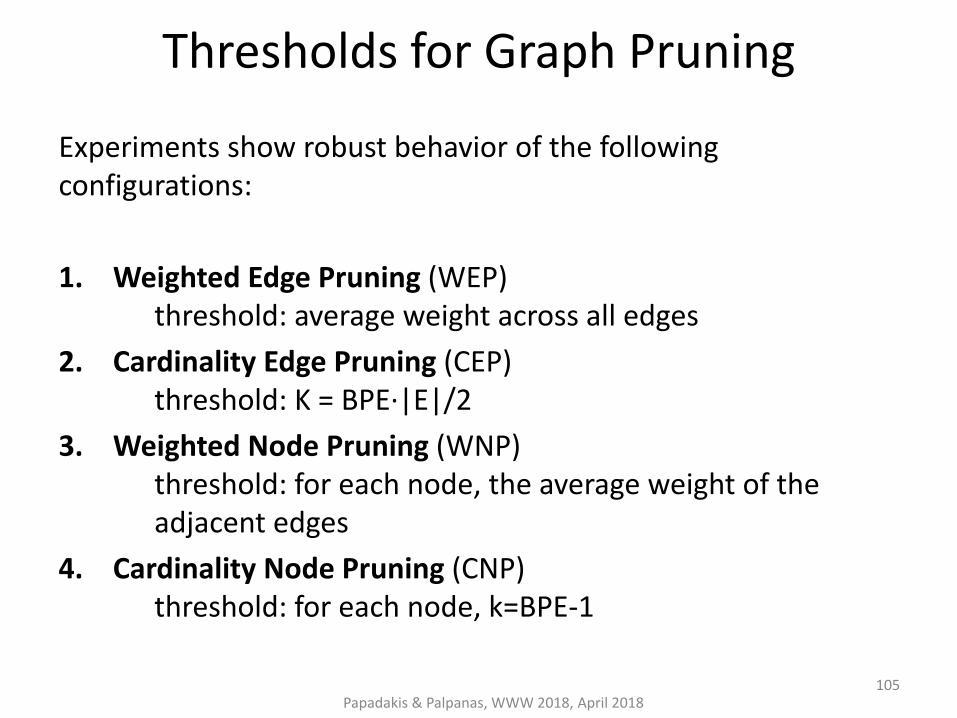
Thresholds for Graph Pruning
Experiments show robust behavior of the following configurations:
1. Weighted Edge Pruning (WEP) threshold: average weight across all edges
2. Cardinality Edge Pruning (CEP) threshold: K = BPE∙|E|/2
3. Weighted Node Pruning (WNP) threshold: for each node, the average weight of the adjacent edges
4. Cardinality Node Pruning (CNP) threshold: for each node, k=BPE-1
Papadakis & Palpanas, WWW 2018, April 2018 105
Back to Motivation
DBPedia 3.0rc ↔ DBPedia 3.4 Brute-force approach
Comparisons: 2.58 ∙ 1012
Recall: 100% Running time: 1,344 days → 3.7 years
Token Blocking + Block Filtering + Comparison Propagation Overhead time: <30 mins Comparisons: 3.5 ∙ 1010 Recall: 99% Total Running time: 19 days
Token Blocking + Block Filtering + Meta-blocking Overhead time: 4 hours Comparisons: 8.95 ∙ 106 Recall: 92% Total Running time: 5 hours
Papadakis & Palpanas, WWW 2018, April 2018
Block Building
Comparison Cleaning
E B Block Cleaning
106

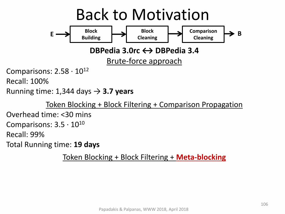
Back to Motivation
DBPedia 3.0rc ↔ DBPedia 3.4 Brute-force approach
Comparisons: 2.58 ∙ 1012
Recall: 100% Running time: 1,344 days → 3.7 years
Token Blocking + Block Filtering + Comparison Propagation Overhead time: <30 mins Comparisons: 3.5 ∙ 1010 Recall: 99% Total Running time: 19 days
Token Blocking + Block Filtering + Meta-blocking Overhead time: 4 hours Comparisons: 8.95 ∙ 106 Recall: 99% Total Running time: 10 hours
Papadakis & Palpanas, WWW 2018, April 2018
Block Building
Comparison Cleaning
E B Block Cleaning
107
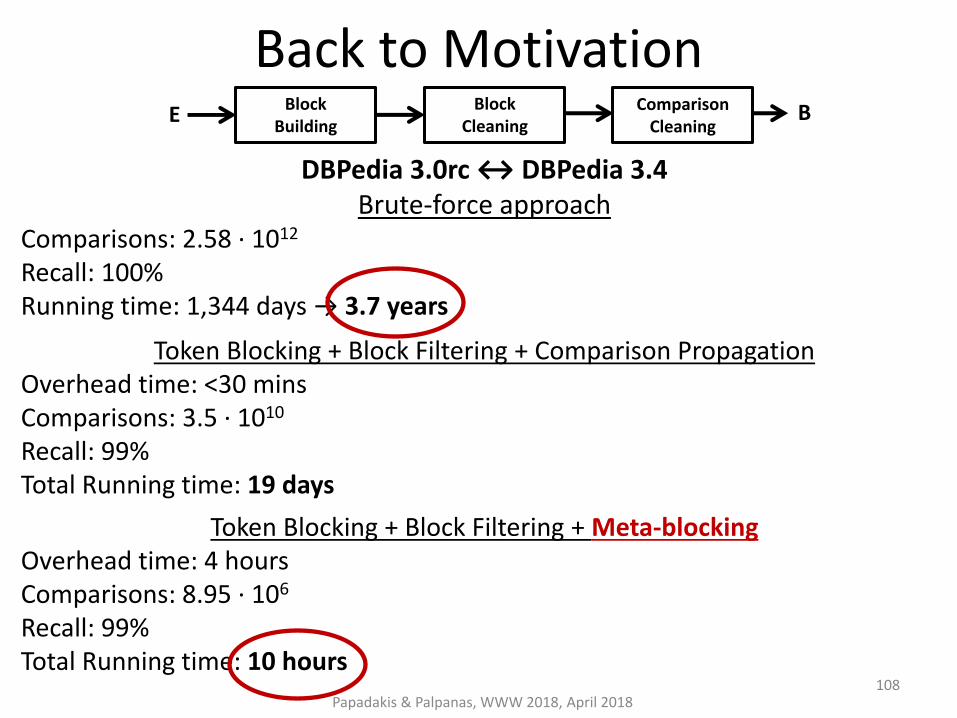
Back to Motivation
DBPedia 3.0rc ↔ DBPedia 3.4 Brute-force approach
Comparisons: 2.58 ∙ 1012
Recall: 100% Running time: 1,344 days → 3.7 years
Token Blocking + Block Filtering + Comparison Propagation Overhead time: <30 mins Comparisons: 3.5 ∙ 1010 Recall: 99% Total Running time: 19 days
Token Blocking + Block Filtering + Meta-blocking Overhead time: 4 hours Comparisons: 8.95 ∙ 106 Recall: 99% Total Running time: 10 hours
Papadakis & Palpanas, WWW 2018, April 2018
Block Building
Comparison Cleaning
E B Block Cleaning
108

Meta-blocking Challenges: Time Efficiency
Bottleneck: edge weighting
• Depends on 𝐵 & BPE
– 𝐸 = 3.4 × 10⁶ , 𝐵 = 4 × 10¹⁰, BPE=15 → 3 hours
– 𝐸 = 7.4 × 10⁶ , 𝐵 = 2 × 10¹¹, BPE=40 → 186 hours
Papadakis & Palpanas, WWW 2018, April 2018 109

Enhancing Meta-blocking Time Efficiency
1. Block Filtering
r = 0.8 → 4 times faster processing, on average
reduces both ||B|| and BPE
2. Optimized Edge Weighting [Papadakis et. al., EDBT 2016]
Entity-based instead of Block-based implementation
An order of magnitude faster processing, in combination with Block Filtering
3. Multi-core Meta-blocking
Commodity hardware
4. Parallel Meta-blocking
Hadoop Cluster
Papadakis & Palpanas, WWW 2018, April 2018 110

Multi-core Meta-blocking [Papadakis et. al, Semantics 2017]
Two types of methods:
• Block-based
• Entity-based
Fork-join approach:
• computational cost split into set of chunks* placed in an array, with an index indicating next chunk to be processed
• Every thread retrieves current value of index and assigned to process corresponding chunk
*chunk = individual items* or a non-overlapping set of items
*item = an individual block or an individual entity
Papadakis & Palpanas, WWW 2018, April 2018 111

Parallelization Strategies
Depending on the definition of chunks, we defined the following parallelization strategies:
1. Random parallelization → individual items in arbitrary order
2. Naïve Parallelization → individual items sorted by cost (#comparisons)
3. Partition Parallelization → an arbitrary number of non-overlapping groups of items with the same computational cost
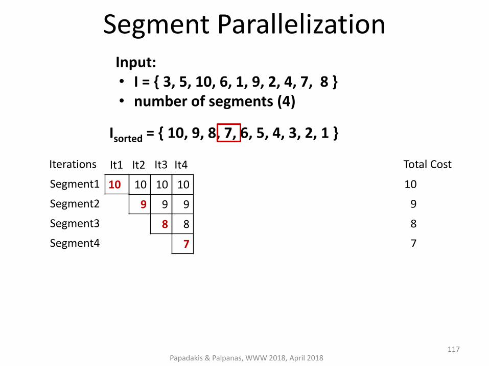
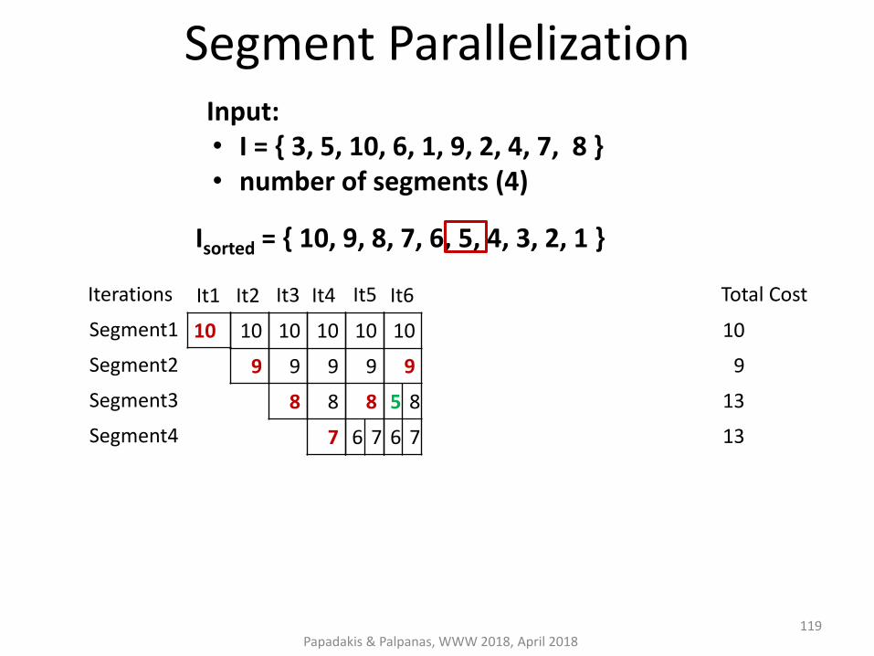
4. Segment Parallelization → #cores non-overlapping groups of items with the same computational cost
Papadakis & Palpanas, WWW 2018, April 2018 112

Segment Parallelization
Papadakis & Palpanas, WWW 2018, April 2018
Input: • I = { 3, 5, 10, 6, 1, 9, 2, 4, 7, 8 } • number of segments (4)
113
Isorted = { 10, 9, 8, 7, 6, 5, 4, 3, 2, 1 }

Segment Parallelization
Papadakis & Palpanas, WWW 2018, April 2018
10 Segment1
It1 Iterations Total Cost
10
Input: • I = { 3, 5, 10, 6, 1, 9, 2, 4, 7, 8 } • number of segments (4)
114
Isorted = { 10, 9, 8, 7, 6, 5, 4, 3, 2, 1 }

Segment Parallelization
Papadakis & Palpanas, WWW 2018, April 2018
10
9
10 Segment1
Segment2
It1 It2 Iterations Total Cost
10
9
Input: • I = { 3, 5, 10, 6, 1, 9, 2, 4, 7, 8 } • number of segments (4)
115
Isorted = { 10, 9, 8, 7, 6, 5, 4, 3, 2, 1 }

Segment Parallelization
Papadakis & Palpanas, WWW 2018, April 2018
10
9
8
10
9
10 Segment1
Segment2
Segment3
It1 It2 It3 Iterations Total Cost
10
9
8
Input: • I = { 3, 5, 10, 6, 1, 9, 2, 4, 7, 8 } • number of segments (4)
116
Isorted = { 10, 9, 8, 7, 6, 5, 4, 3, 2, 1 }
Segment Parallelization
Papadakis & Palpanas, WWW 2018, April 2018
10
9
8
10
9
8
7
10
9
10 Segment1
Segment2
Segment3
Segment4
It1 It2 It3 It4 Iterations Total Cost
10
9
8
7
Input: • I = { 3, 5, 10, 6, 1, 9, 2, 4, 7, 8 } • number of segments (4)
117
Isorted = { 10, 9, 8, 7, 6, 5, 4, 3, 2, 1 }

Segment Parallelization
Papadakis & Palpanas, WWW 2018, April 2018
10
9
8
10
9
8
7
10
9
10 Segment1
Segment2
Segment3
Segment4
10
9
8
6 7
It1 It2 It3 It4 It5 Iterations Total Cost
10
9
8
13
Input: • I = { 3, 5, 10, 6, 1, 9, 2, 4, 7, 8 } • number of segments (4)
118
Isorted = { 10, 9, 8, 7, 6, 5, 4, 3, 2, 1 }
Segment Parallelization
Papadakis & Palpanas, WWW 2018, April 2018
10
9
8
10
9
8
7
10
9
10 Segment1
Segment2
Segment3
Segment4
10
9
5 8
6 7
10
9
8
6 7
It1 It2 It3 It4 It5 It6 Iterations Total Cost
10
9
13
13
Input: • I = { 3, 5, 10, 6, 1, 9, 2, 4, 7, 8 } • number of segments (4)
119
Isorted = { 10, 9, 8, 7, 6, 5, 4, 3, 2, 1 }

Segment Parallelization
Papadakis & Palpanas, WWW 2018, April 2018
10
9
8
10
9
8
7
10
9
10 Segment1
Segment2
Segment3
Segment4
10
9
5 8
6 7
10
4 9
5 8
6 7
10
9
8
6 7
It1 It2 It3 It4 It5 It6 It7 Iterations Total Cost
10
13
13
13
Input: • I = { 3, 5, 10, 6, 1, 9, 2, 4, 7, 8 } • number of segments (4)
120
Isorted = { 10, 9, 8, 7, 6, 5, 4, 3, 2, 1 }

Segment Parallelization
Papadakis & Palpanas, WWW 2018, April 2018
10
9
8
10
9
8
7
10
9
10 Segment1
Segment2
Segment3
Segment4
10
9
5 8
6 7
10
4 9
5 8
6 7
10
9
8
6 7
3 10
4 9
5 8
6 7
It1 It2 It3 It4 It5 It6 It7 It8 Iterations Total Cost
13
13
13
13
Input: • I = { 3, 5, 10, 6, 1, 9, 2, 4, 7, 8 } • number of segments (4)
121
Isorted = { 10, 9, 8, 7, 6, 5, 4, 3, 2, 1 }

Segment Parallelization
Papadakis & Palpanas, WWW 2018, April 2018
10
9
8
10
9
8
7
10
9
10 Segment1
Segment2
Segment3
Segment4
10
9
5 8
6 7
10
4 9
5 8
6 7
10
9
8
6 7
3 10
4 9
5 8
6 7
3 10
4 9
5 8
6 2 7
It1 It2 It3 It4 It5 It6 It7 It8 It9 Iterations Total Cost
13
13
13
15
Input: • I = { 3, 5, 10, 6, 1, 9, 2, 4, 7, 8 } • number of segments (4)
122
Isorted = { 10, 9, 8, 7, 6, 5, 4, 3, 2, 1 }

Segment Parallelization
Papadakis & Palpanas, WWW 2018, April 2018
10
9
8
10
9
8
7
10
9
10 Segment1
Segment2
Segment3
Segment4
10
9
5 8
6 7
10
4 9
5 8
6 7
10
9
8
6 7
3 10
4 9
5 8
6 7
3 10
4 9
5 8
6 2 7
3 10
4 9
5 1 8
6 2 7
It1 It2 It3 It4 It5 It6 It7 It8 It9 It10 Iterations Total Cost
13
13
14
13
Input: • I = { 3, 5, 10, 6, 1, 9, 2, 4, 7, 8 } • number of segments (4)
Time complexity: O(n log n)
123
Isorted = { 10, 9, 8, 7, 6, 5, 4, 3, 2, 1 }

Execution Plan
Papadakis & Palpanas, WWW 2018, April 2018
Total valid comparisons
Merge
Initialization
MWEP MWNP MCEP MCNP Initialize chunk array and N threads.
Initialize chunk array and N threads.
Initialize chunk array and N threads. Estimate K.
Each thread computes local aggregate edge weight and #comparisons
Estimate average edge weight
Each thread stores the total weight and #comparisons per entity in two arrays
Check and keep valid comparisons above the weight threshold
Output total valid comparisons
Merge the 2 arrays to compute the average edge weight of each node
Check and keep valid comparisons above the weight threshold of any adjacent node
Output total valid comparisons
Every thread stores the k top-weighted edges for every processed entity in a priority queue
Output the comparisons that are among the k top-weighted ones for any of the adjacent entities
Stage 1
Stage 2
Each thread stores the K top-weighted edges in the processed chunks in a priority queue
Output the overall K top-weighted comparisons
Initialize chunk array and N threads. Estimate k.
th1 th2 th3 thN …
th1 th2 th3 thN …
124

Experimental Evaluation - Datasets
Original Datasets
DBPedia 3.0rc
DBPedia 3.4
Entities 1,190,733 2,164,040
Duplicates 892,579
Triples 1.69∙107 3.50∙107
Predicates 30,757 52,554
Brute-force 2.58∙1012
Papadakis & Palpanas, WWW 2018, April 2018
Blocks Input Output (CNP)
Blocks 1,239,066 1,190,733
Comparisons 1.30∙1010 3.30∙107
Detected Matches
890,817 859,554
Recall 0.998 0.963
Precision 6.86∙10−5 2.61∙10−2
System: Server running Ubuntu 12.04, 32GB RAM and 2 Intel Xeon E5620 processors, each having 4 physical cores and 8 logical cores at 2.40GHz.
125
token blocking + block purging + block filtering
token blocking + block purging + block filtering +
meta-blocking CNP

Experimental Evaluation – CNP Wall Clock Time
Papadakis & Palpanas, WWW 2018, April 2018
Single-threaded time = 3.5 hours RB=Random, block-based parallelization NB=Naïve, block-based parallelization PB=Partition, block-based parallelization SB=Segment, block-based parallelization RE=Random, entity-based parallelization NE=Naïve, entity-based parallelization PE=Partition, entity-based parallelization SE=Segment, entity-based parallelization 15 min
126

Experimental Evaluation – CNP Speedup
Papadakis & Palpanas, WWW 2018, April 2018
RB=Random, block-based parallelization NB=Naïve, block-based parallelization PB=Partition, block-based parallelization SB=Segment, block-based parallelization RE=Random, entity-based parallelization NE=Naïve, entity-based parallelization PE=Partition, entity-based parallelization SE=Segment, entity-based parallelization
127

Meta-blocking Challenges: Effectiveness
Problem:
• Simple pruning rules
Solutions:
• Unsupervised methods – BLAST
• Integrates schema information
• Supervised methods – Supervised Meta-blocking (SMB)
• utilizes feature-based classification of blocking-graph edges
– BLOSS
• minimizes the size of the required training set
Papadakis & Palpanas, WWW 2018, April 2018 128

BLAST [Simonini et. al., VLDB 2017]
• Goal: improve the edge weighting and pruning in unsupervised WNP with loose schema information
• Solution:
It works for Dirty ER, as well.
Papadakis & Palpanas, WWW 2018, April 2018 129
Courtesy of Giovanni Simonini

Similar to Attribute Clustering:
1. Each attribute is represented as the set of its possible values
2. Builds a (bipartite*) graph with one node for every attribute
3. There is an edge for every pair of attributes with similarity > 0
4. Each connected component is an attribute cluster
* In the case of Clean-Clean ER.
The original Attribute Clustering does
not scale to thousands of attributes
→ very inefficient
BLAST employs LSH to reduce the
time complexity (for JaccardSim)
• Scales well to hundred of
thousands attributes
• Simultaneously estimates
aggregate entropy per cluster
Loose Schema Information Extraction
Papadakis & Palpanas, WWW 2018, April 2018 130
Courtesy of Giovanni Simonini

Loosely Schema-aware Meta-blocking
1. BLAST improves edge weighting as follows: every edge → several blocking keys (tokens) → multiple attribute names → w(eij)=aggregate entropy∙Pearson’s χ2
2. BLAST improves edge pruning in two ways: – Local weight threshold independent of the size of each node neighborhood
(i.e., number of edges):
𝜃𝑖 =𝑎𝑟𝑔𝑚𝑎𝑥𝑖 𝑤(𝑒𝑖𝑗)
2
– An edge 𝑒𝑖𝑗 is retained if 𝑤(𝑒𝑖𝑗) ≥𝜃𝑖+𝜃𝑗
2 .
Papadakis & Palpanas, WWW 2018, April 2018 131
Courtesy of Giovanni Simonini

Example – Original Meta-blocking
Papadakis & Palpanas, WWW 2018, April 2018
Entity Collection Token Blocking
Blocking Graph New Collection Pruned Graph
132 Courtesy of Giovanni Simonini

Example – Meta-blocking over Attribute Clustering
Papadakis & Palpanas, WWW 2018, April 2018
Entity Collection Attribute Clustering
Blocking Graph
name,f.name,
s.name
Other
Attributes
C1 C2 New Collection Pruned Graph
Attribute Clusters
133 Courtesy of Giovanni Simonini
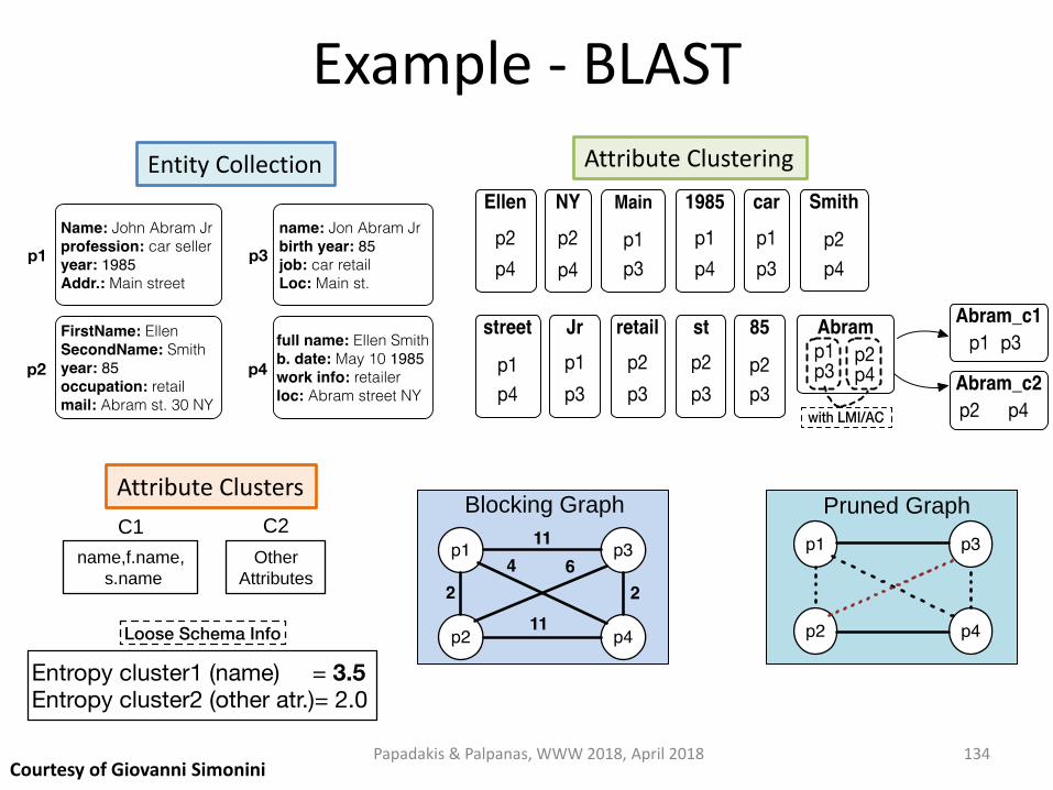
Example - BLAST
Papadakis & Palpanas, WWW 2018, April 2018
Entity Collection Attribute Clustering
Blocking Graph
name,f.name,
s.name
Other
Attributes
C1 C2 New Collection Pruned Graph
Attribute Clusters
134 Courtesy of Giovanni Simonini

Supervised Meta-blocking [Papadakis et. al., VLDB 2014]
Goal:
more accurate and comprehensive methodology for
pruning the edges of the blocking graph
Solution:
- model edge pruning as a classification task per edge
- two classes: “likely match”, “unlikely match”
Open issues:
• Classification Features
• Training Set
• Classification Algorithms & Configuration
Papadakis & Palpanas, WWW 2018, April 2018 135

Requirements:
1. Generic 2. Effective
3. Efficient 4. Minimal
Classification Features
Papadakis & Palpanas, WWW 2018, April 2018 136

Feature Engineering
CF-IBF = # of Common Blocks × Inverse Block Frequency per entity RACCB = Sum of Inverse Block Sizes We examined all 63 possible combinations to find the minimal set of features, which comprises the first four features.
Papadakis & Palpanas, WWW 2018, April 2018 137

Training Set
Challenge:
binary classification with heavily imbalanced classes
Solutions:
1. Oversampling
2. Cost-sensitive learning
3. Ensemble learning
4. Undersampling
– Sample size equal to 5% of the minority class.
Papadakis & Palpanas, WWW 2018, April 2018 138

Classification Algorithms
Weighted Edge Pruning (WEP) • compatible with any classifier
• we selected 4 state-of-the-art:
1. Naïve Bayes
2. Bayesian Networks
3. C4.5 Decision Trees
4. Support Vector Machines
Cardinality Edge Pruning (CEP) &
Cardinality Node Pruning (CNP) • compatible with probabilistic classifiers
• we selected Naïve Bayes, Bayesian Networks
Configuration For selected features and sample size, classifiers are robust with respect to their internal parameters
Papadakis & Palpanas, WWW 2018, April 2018 139

Experiments
Papadakis & Palpanas, WWW 2018, April 2018 140
recall

Experiments
recall almost unaffected
Papadakis & Palpanas, WWW 2018, April 2018 141

Experiments
recall almost unaffected
running time
Papadakis & Palpanas, WWW 2018, April 2018 142
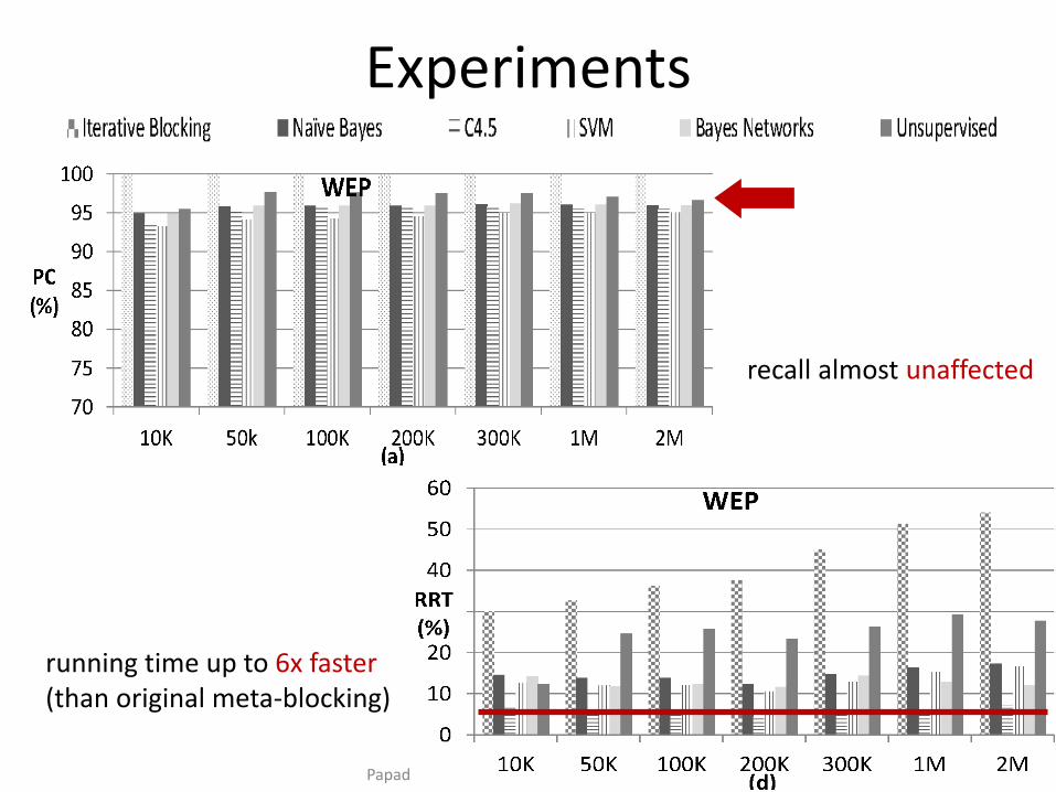
Experiments
recall almost unaffected
running time up to 6x faster (than original meta-blocking)
Papadakis & Palpanas, WWW 2018, April 2018 143

BLOSS [Dal Bianco et al., Information Systems, 2018]
Goal:
minimize the labelling effort for training Supervised Meta-blocking
Solution:
meta-BLOcking Sampling Selection
- involves a novel sampling methodology
- combines it with active learning
Key feature:
• removes outliers to improve recall
Papadakis & Palpanas, WWW 2018, April 2018 144
Courtesy of Guilherme Dal Bianco

BLOSS Outline
It comprises three steps:
1. Definition of Similarity Levels and Random Sampling – pre-selects candidate pairs using a metric that assesses the potential
of a pair being a match
– level-based sampling ensures diversity
2. Selection of Pairs for Labeling – applies active learning applied to the pre-selected pairs
3. Pruning Non-Matching Outliers – filters out noisy non-matching pairs that have been labeled
Papadakis & Palpanas, WWW 2018, April 2018 145 Courtesy of Guilherme Dal Bianco
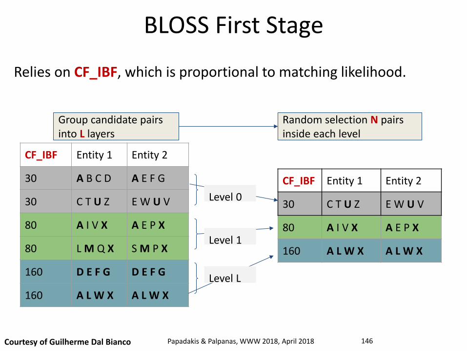
Group candidate pairs into L layers
Random selection N pairs inside each level
CF_IBF Entity 1 Entity 2
30 A B C D A E F G
30 C T U Z E W U V
80 A I V X A E P X
80 L M Q X S M P X
160 D E F G D E F G
160 A L W X A L W X
CF_IBF Entity 1 Entity 2
30 C T U Z E W U V
80 A I V X A E P X
160 A L W X A L W X
Level L
Level 1
Level 0
BLOSS First Stage
Relies on CF_IBF, which is proportional to matching likelihood.
Courtesy of Guilherme Dal Bianco Papadakis & Palpanas, WWW 2018, April 2018 146

BLOSS First Stage – Layers distribution
• first levels probably include more non-matching pairs • last levels group more matching pairs
Courtesy of Guilherme Dal Bianco
increasing CF_IBF
Papadakis & Palpanas, WWW 2018, April 2018 147
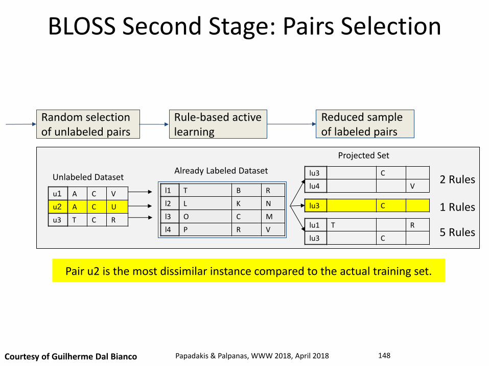
Random selection of unlabeled pairs
u1 A C V
u2 A C U
u3 T C R
l1 T B R
l2 L K N
l3 O C M
l4 P R V
lu3 C
lu4 V
lu3 C
lu1 T R
lu3 C
Unlabeled Dataset Already Labeled Dataset
Projected Set
2 Rules
1 Rules
5 Rules
Pair u2 is the most dissimilar instance compared to the actual training set.
Rule-based active learning
Reduced sample of labeled pairs
BLOSS Second Stage: Pairs Selection
Courtesy of Guilherme Dal Bianco Papadakis & Palpanas, WWW 2018, April 2018 148

BLOSS Third Stage: Outliers Pruning
Goal: remove noise, while maximizing recall.
Courtesy of Guilherme Dal Bianco Papadakis & Palpanas, WWW 2018, April 2018 149

Pruning Threshold: average Jaccard similarity of non-matching labelled instances.
BLOSS Third Stage – Part B
DBLP-Scholar DBLP-ACM Synthetic Dataset
Courtesy of Guilherme Dal Bianco Papadakis & Palpanas, WWW 2018, April 2018 150

Measures: RRT = Relative running time wrt to original blocking (without Meta-blocking) ΔPC = Reduction in recall wrt to original blocking ΔPQ = Increase in precision wrt to original blocking
BLOSS achieves a reduction in the training set size of around 40 times.
BLOSS Effectiveness & Time Efficiency
Courtesy of Guilherme Dal Bianco Papadakis & Palpanas, WWW 2018, April 2018 151

Comparative Analysis of Approximate Blocking Techniques [Papadakis et. al., VLDB 2016]
• employed 3 sub-tasks of blocking
Papadakis & Palpanas, WWW 2018, April 2018
Block Building
Comparison Cleaning
E B Block Cleaning
Lazy
blocking
methods
Block-refinement
methods
Comparison-
refinement
methods
Proactive blocking methods
152

• considered 5 lazy and 7 proactive blocking methods
Papadakis & Palpanas, WWW 2018, April 2018
Comparative Analysis of Approximate Blocking Techniques [Papadakis et. al., VLDB 2016]
153

Experimental Analysis Setup
• Block Cleaning methods: 1. Block Purging
2. Block Filtering
• Comparison Cleaning methods: 1. Comparison Propagation
2. Iterative Blocking
3. Meta-blocking
Papadakis & Palpanas, WWW 2018, April 2018 154
Experimental Analysis Setup
• Exhaustive parameter tuning to identify two configurations for each method:
1. Best configuration per dataset → maximizes 𝒂 𝑩, 𝑬 = 𝑹𝑹 𝑩, 𝑬 ∙ 𝑷𝑪(𝑩, 𝑬)
2. Default configuration → highest average 𝒂 across all datasets
• Extensive experiments measuring effectiveness and time efficiency over 5 real datasets (up to 3.3M entities).
• Scalability analysis over 7 synthetic datasets (up to 2M entities).
Papadakis & Palpanas, WWW 2018, April 2018 155

Effectiveness of Lazy Methods on DBPedia
Papadakis & Palpanas, WWW 2018, April 2018 156

Effectiveness of Lazy Methods on DBPedia
Papadakis & Palpanas, WWW 2018, April 2018
Token-blocking and Meta-blocking
157

Time Efficiency of Lazy Methods on DBPedia
Papadakis & Palpanas, WWW 2018, April 2018 158

Time Efficiency of Lazy Methods on DBPedia
Papadakis & Palpanas, WWW 2018, April 2018
Token-blocking and Meta-blocking
159

Effectiveness of Proactive methods on DBPedia
Papadakis & Palpanas, WWW 2018, April 2018 160

Effectiveness of Proactive methods on DBPedia
Papadakis & Palpanas, WWW 2018, April 2018
Suffix-arrays and Meta-blocking
161

Time Efficiency of Proactive Methods on DBPedia
Papadakis & Palpanas, WWW 2018, April 2018 162

Time Efficiency of Proactive Methods on DBPedia
Papadakis & Palpanas, WWW 2018, April 2018
Suffix-arrays and Meta-blocking
163

Papadakis & Palpanas, WWW 2018, April 2018
Part 6:
Entity Matching
164

165
Preliminaries
• Estimates the similarity of candidate matches.
• Input – Pruned Blocking Graph
• Nodes → entities
• Edges → candidate matches
– Or, a set of blocks
• Every comparison in any block is a candidate match
• Output – Similarity Graph
• Nodes → entities
• Edges → candidate matches
• Edge weights → similarity of entity profiles (+neighbors)
Papadakis & Palpanas, WWW 2018, April 2018

Naïve Approach
• For each pair of entities, e1-e2
– Estimate aggregate similarity based on: • attribute values
• neighbors
• external knowledge
• combination of above
– If similarity > threshold → match! (unsupervised)
– If classifierDecision(e1,e2) = true → match! (supervised)
Papadakis & Palpanas, WWW 2018, April 2018 166

167
Group Linkage [On et al., ICDE 2007]
• Often, “entity” is represented as a uniquely identified group of information
• In structured data:
– An author with a group of publication records
– A household in a census survey with a group of family members
• In semi-structured data:
– Every entity is a group of name-value pairs.
Group Linkage Problem: to determine if two entities represented as groups are approximately the same or not
Papadakis & Palpanas, WWW 2018, April 2018 Courtesy of Dongwon Lee

168
Group Linkage: Popular Group Similarity
Jaccard
• Intuitive, cheap to run
• Error-prone
21
2121 ),(
gg
ggggsim
Bipartite Matching
Cardinality
Weighted
Rich
Expensive to run
Q: Can we combine Jaccard and Bipartite Matching for Group Linkage?
Papadakis & Palpanas, WWW 2018, April 2018 Courtesy of Dongwon Lee

169
Group Linkage: Intuition for Better Similarity
• Two groups are similar if:
– A large fraction of elements in the two groups form matching element pairs
– There is high enough similarity between matching pairs of individual elements that constitute the two groups
Papadakis & Palpanas, WWW 2018, April 2018 Courtesy of Dongwon Lee

170
Group Linkage: Group Similarity
• Two groups of elements:
– g1 = {r11, r12, …, r1m1}, g2 = {r21, r22, …, r2m2}
– The group measure BM is the normalized weight of the maximum bipartite matching M in the bipartite graph (N = g1 U g2, E=g1 X g2)
such that
– BM(g1, g2) ≥ θ
Mmm
rrsimggBM
Mrr ji
sim
ji
21
),( 21
2,1,
21
)),(()(
)( 2,1 ji rrsim
21
2121 ),(
gg
ggggsim
Papadakis & Palpanas, WWW 2018, April 2018 Courtesy of Dongwon Lee
user-defined parameters

171
Group Linkage: Example ( )
3.0
9.0,3.0
0.7 0.4 0.5 0.9 0.2 0.3 g1 g2
0.7
0.4
0.5
0.9
M: max-weight bipartite matching
0.7
0.4
0.5
0.9
sparse bipartite graph
53.03
6.1
223
7.09.0
)),(()(
21
),( 21
2,1,
21
Mmm
rrsimggBM
Mrr ji
sim
ji
Therefore, g1 <> g2 !
Papadakis & Palpanas, WWW 2018, April 2018 Courtesy of Dongwon Lee

172
Group Linkage: Challenge
• Each BM group measure uses the maximum weight bipartite matching – Bellman-Ford: O(V2E)
– Hungarian: O(V3)
• Large number of groups to match – O(NM)
…
…
N M Papadakis & Palpanas, WWW 2018, April 2018 Courtesy of Dongwon Lee

173
Group Linkage: Solution: Greedy matching
• Bipartite matching computation is expensive because of the requirement
– No node in the bipartite graph can have more than one edge incident on it
• Let’s relax this constraint:
– For each element ei in g1, find an element ej in g2 with the highest element-level similarity S1
– For each element ej in g2, find an element ei in g1 with the highest element-level similarity S2
Papadakis & Palpanas, WWW 2018, April 2018 Courtesy of Dongwon Lee

Papadakis & Palpanas, WWW 2018, April 2018
174
Upper/Lower Bounds
2121
21),( 21
2,1,
21
)),(()(
SSmm
rrsimggUB
SSrr ji
sim
ji
2121
21),( 21
2,1,
21
)),(()(
SSmm
rrsimggLB
SSrr ji
sim
ji
Mmm
rrsimggBM
Mrr ji
sim
ji
21
),( 21
2,1,
21
)),(()(
Courtesy of Dongwon Lee

Papadakis & Palpanas, WWW 2018, April 2018
175
Theorem & Algorithm
• ELSE IF LB(g1,g2) ≥ θ → BM(g1,g2) ≥ θ → g1≈ g2
• ELSE, compute BM(g1,g2)
IF UB(g1,g2) < θ → BM(g1,g2) < θ → g1 ≠ g2
)()( 2,1,2,1, ggBMggLB simsim
)()( 2,1,2,1, ggUBggBM simsim
Goal: BM(g1,g2) ≥ θ
Theorem 1
Theorem 2
Courtesy of Dongwon Lee

Iterative Approaches [Stefanidis et al., WWW 2014]
• Increase recall by updating related entities upon detection of a new match
• Core principles:
– Transitivity: if match(e1,e2)=true & match(e2,e3)=true → match(e1,e3)=true
– Duplicate dependency: if entities of one type (e.g., authors) are matches, related entities of another type (e.g., publications) are more likely to be matches, too.
– Merge dependency: if match(e1,e2)=true, replace e1 & e2
with e12 and compare again with all other similar entities.
Papadakis & Palpanas, WWW 2018, April 2018 176

Swoosh [Benjelloun et al., VLDBJ 2009]
• Iterative approach crafted for relational data. • Relies on two functions: match (m) and merge (μ) • Algorithm outline: while the input list I is not empty
– e1 ← I.removeFirstRecord() – matchFound = false – for each record in the output list , e2 ∈ 𝑶
• if m (e1, e2 ) == true then – O.remove ( e2 ) – I .add( μ ( e1 , e2 ) ) – matchFound = true – break
– if matchFound == false – O.add( e1 )
Papadakis & Palpanas, WWW 2018, April 2018 177

Swoosh Efficiency [Benjelloun et al., VLDBJ 2009]
• Higher efficiency (fewer calls to match & merge) when specific properties hold: – Idempotence:
m(ei, ei) = true, μ(ei, ei) = ei
– Commutativity:
m(ei, ej) = M(ej, ei), μ(ei, ej) = μ(ej, ei)
– Associativity:
μ(ei, μ(ej, ek)) = μ(μ(ei,ej), ek)
– Representativity:
if μ(ei, ei) = ek & m(ei, el) = true → m(ek, el) = true
Papadakis & Palpanas, WWW 2018, April 2018
178

Simple Greedy Matching (SiGMa) [Lacoste-Julien et al., KDD 2013]
• relies on the 1-1 assumption of Clean-Clean ER – once a match is identified, it never needs to be compared to other entities
• exploits relationship graph to score decisions and to propose candidates
• can easily use tailored similarity measures
• iterative algorithm – provides natural tradeoff between precision & recall as well as between
computation and recall
• simplicity & greediness → high time efficiency
• exhibits high effectiveness, as well
Papadakis & Palpanas, WWW 2018, April 2018 179
Courtesy of Simon Lacoste-Julien

SiGMa intuition
SiGMa uses neighbors for: 1) scoring candidates
2) suggest candidates (iterative blocking)
Papadakis & Palpanas, WWW 2018, April 2018 180
Courtesy of Simon Lacoste-Julien

Quadratic Assignment objective
pairwise similarity score graph compatibility score:
counts the number of valid neighbors which are currently matched (context)
normalizing weight
Papadakis & Palpanas, WWW 2018, April 2018 181
Courtesy of Simon Lacoste-Julien

SiGMa similarity scores • Increase in objective when matching pair (i,j):
• Pairwise similarity score (could use others):
• Similarity on string representation of entities: – Jaccard measure on words in common + smoothing + weights (TF-IDF
weights)
– Property similarity measure: also smoothed weighted Jaccard similarity measure between sets of properties, with additional similarity on literals:
Papadakis & Palpanas, WWW 2018, April 2018 182
Courtesy of Simon Lacoste-Julien

SiGMa Algorithm
1. Start with seed match 2. Put neighbors in S 3. At each iteration:
a) pick new pair in S which max. increase b) add new neighbors in S
4. Stop when variation below threshold
Papadakis & Palpanas, WWW 2018, April 2018 183
Courtesy of Simon Lacoste-Julien

PARIS [Suchanek et al., PVLDB 2011]
• Probabilistic, iterative, parameter-free method
• Collective approach for holistically aligning entities, relations and classes – applicable to Clean-Clean ER (for knowledge graphs)
• Algorithm outline: 1. Fix equalities for literals (numbers, or strings)
2. Set equalities for relations to a small initial value
3. Iterate the estimations for relations and entities until convergence (*)
4. Compute the estimations for classes
(*) There is no proof for convergence, but it seems to happen
Papadakis & Palpanas, WWW 2018, April 2018 184
Courtesy of Fabian Suchanek

PARIS – Part B • Equality of Literals
– Pr(x ≡ y) := (x = y) ? 1 : 0
• Equality of Entities – Based on the local inverse functionality of a relation r
1/#the number of entities with a given argument for r
– The probability of a relation being inverse functional is the harmonic mean of the local inverse functionalities
– Two entities are matching if they share at least one argument for a highly inverse functional relation
• Equality of Classes – Based on the subsumption probability: if all entities of one class are entities
of the other, then the former subsumes the latter
• Equality of Relations • Based on the probability that one relation is sub-property of the other
Papadakis & Palpanas, WWW 2018, April 2018 185

Synthesizing Entity Matching Rules
Machine Learning System
186
Best F-measure Not interpretable
Rule-Based Approach
Lower F-measure Interpretable
Courtesy of Paolo Papotti Papadakis & Palpanas, WWW 2018, April 2018

Synthesizing Entity Matching Rules Using Examples [Singh et al., PVLDB 2017]
187
Program Synthesis
Tuneable trade off between F1 and complexity
Courtesy of Paolo Papotti Papadakis & Palpanas, WWW 2018, April 2018
General Boolean Formula (GBF): can include arbitrary attribute matching predicates combined by conjunctions, disjunctions, and negations

Synthesizing Entity Matching Rules Using Examples [Singh et al., PVLDB 2017]
F-measure comparable to DTs depth 10 and SVM
188 Courtesy of Paolo Papotti Papadakis & Palpanas, WWW 2018, April 2018

Papadakis & Palpanas, WWW 2018, April 2018
Part 7:
Entity Clustering
189

190
Preliminaries
• Partitions the matched pairs into equivalence clusters → groups of entity profiles describing the same real-world object
• Input – Similarity Graph:
• Nodes → entities
• Edges → candidate matches
• Edge weights → likelihood of matching entities
• Output – Equivalence Clusters
Papadakis & Palpanas, WWW 2018, April 2018 190
191
Clustering Algorithms for Clean-Clean ER
• Unique Mapping Clustering [Lacoste-Julien et al., KDD 2013]
[Suchanek et al., PVLDB 2011]
– Relies on 1-1 constraint • 1 entity from first dataset matches to 1 entity from second
– Sorts all edges in decreasing weight
– Starting from the top, each edge corresponds to a pair of duplicates if:
• None of the adjacent entities has already been matched
• predefined threshold < edge weight
Papadakis & Palpanas, WWW 2018, April 2018 191
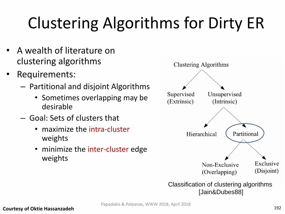
192
Clustering Algorithms for Dirty ER
• A wealth of literature on clustering algorithms
• Requirements: – Partitional and disjoint Algorithms
• Sometimes overlapping may be desirable
– Goal: Sets of clusters that
• maximize the intra-cluster weights
• minimize the inter-cluster edge weights
Classification of clustering algorithms
[Jain&Dubes88]
Papadakis & Palpanas, WWW 2018, April 2018 Courtesy of Oktie Hassanzadeh 192

193
Clustering Algorithms Characteristics [Hassanzadeh et al., VLDB 2009]
• Most important feature
“Unconstrained algorithms”
• I.e. , algorithms that do not require as input: – The number of clusters
– The diameter of the clusters
– Any other domain specific parameters
• Algorithms need to be able to predict the correct number of clusters
Papadakis & Palpanas, WWW 2018, April 2018 Courtesy of Oktie Hassanzadeh 193

194
Clustering Algorithms Characteristics [Hassanzadeh et al., VLDB 2009]
• Need to scale well – Time complexity < O(n2)
• Need to be robust with respect to characteristics of the data – E.g., distribution of the duplicates
• Need to be capable of finding ‘singleton’ clusters – Different from many clustering algorithms
• E.g., algorithms proposed for image segmentation
Papadakis & Palpanas, WWW 2018, April 2018 Courtesy of Oktie Hassanzadeh 194

Single-pass Algorithms [Hassanzadeh et al., VLDB 2009]
• Perform clustering by a single scan of the output of the similarity join (the edges of the graph)
– Partitioning • TRANSITIVE CLOSURE
– CENTER [HGI-WebDB'00]
– MERGE-CENTER [HM-VLDBJ09]
195 Papadakis & Palpanas, WWW 2018, April 2018 Courtesy of Oktie Hassanzadeh 195

Single-pass Algorithms [Hassanzadeh et al., VLDB 2009]
• Perform clustering by a single scan of the output of the similarity join (the edges of the graph)
– Partitioning • TRANSITIVE CLOSURE
– CENTER [HGI-WebDB'00]
– MERGE-CENTER [HM-VLDBJ09]
196
t1
t2
0.71
t3
t5
t8
t4 t7
t6
0.48
0.23
0.26
0.65
0.77
0.30
0.68
Papadakis & Palpanas, WWW 2018, April 2018 Courtesy of Oktie Hassanzadeh 196

Single-pass Algorithms [Hassanzadeh et al., VLDB 2009]
• Perform clustering by a single scan of the output of the similarity join (the edges of the graph)
– Partitioning • TRANSITIVE CLOSURE
– CENTER [HGI-WebDB'00]
– MERGE-CENTER [HM-VLDBJ09]
197
t1
t2
0.71
t3
t5
t8
t4 t7
t6
0.65
0.77
0.68
Papadakis & Palpanas, WWW 2018, April 2018 Courtesy of Oktie Hassanzadeh 197

Single-pass Algorithms [Hassanzadeh et al., VLDB 2009]
• Perform clustering by a single scan of the output of the similarity join (the edges of the graph)
– Partitioning • TRANSITIVE CLOSURE
– CENTER [HGI-WebDB'00]
– MERGE-CENTER [HM-
VLDBJ09]
198
t1
t2
0.71
t3
t5
t8
t4 t7
t6
0.48
0.26
0.65
0.77
0.30
0.68
Papadakis & Palpanas, WWW 2018, April 2018 Courtesy of Oktie Hassanzadeh 198

199
t1
t2
0.71
t3
t5
t8
t7
t6
0.48
0.23
0.26
0.30
t5 t60.65
Star Algorithm [APR-JGraph04]
• Creates star-shaped clusters
– heuristic to approximate problem of finding minimal clique cover of graph
• Similar to CENTER but
– Allows overlapping clusters
– First sorts nodes in descending order of their degrees
Papadakis & Palpanas, WWW 2018, April 2018 Courtesy of Oktie Hassanzadeh 199
200
Ricochet Algorithms [WB-DASFAA’09]
• Ricochet family of algorithms – Based on a strategy that resembles the rippling of stones
thrown in a pond – Combine ideas from the classic K-means algorithm and the
Star algorithm • First selecting seeds (star centers) for the clusters and then
refining the clusters iteratively
– Four unconstrained clustering algorithms, originally proposed for document clustering
• SR, BSR, CR and OCR
– SR and BSR perform a sequential selection of the cluster seeds; CR and OCR perform a concurrent selection of the seeds
Papadakis & Palpanas, WWW 2018, April 2018 Courtesy of Oktie Hassanzadeh 200

201
Min-Cut Clustering [Hassanzadeh et al., VLDB 2009]
• Based on the Cut-Clustering Algorithm [FTT-IM04]
– Finding minimum cuts of edges in the similarity graph after inserting an artificial sink into similarity graph G
t1
t2
0.71
t3
t5
t6
t4
t7
t8
0.48
0.22
0.32
0.230.27
0.57
0.24
0.480.68
s
Papadakis & Palpanas, WWW 2018, April 2018 Courtesy of Oktie Hassanzadeh 201

202
Articulation Point Clustering [Hassanzadeh et al., VLDB 2009]
• A scalable graph partitioning algorithm
• Based on finding articulation points
– Articulation point: a vertex whose removal makes the graph disconnected
• Efficient implementations proposed for identifying chatter in the blogosphere [BCKT-VLDB07]
Papadakis & Palpanas, WWW 2018, April 2018 Courtesy of Oktie Hassanzadeh 202
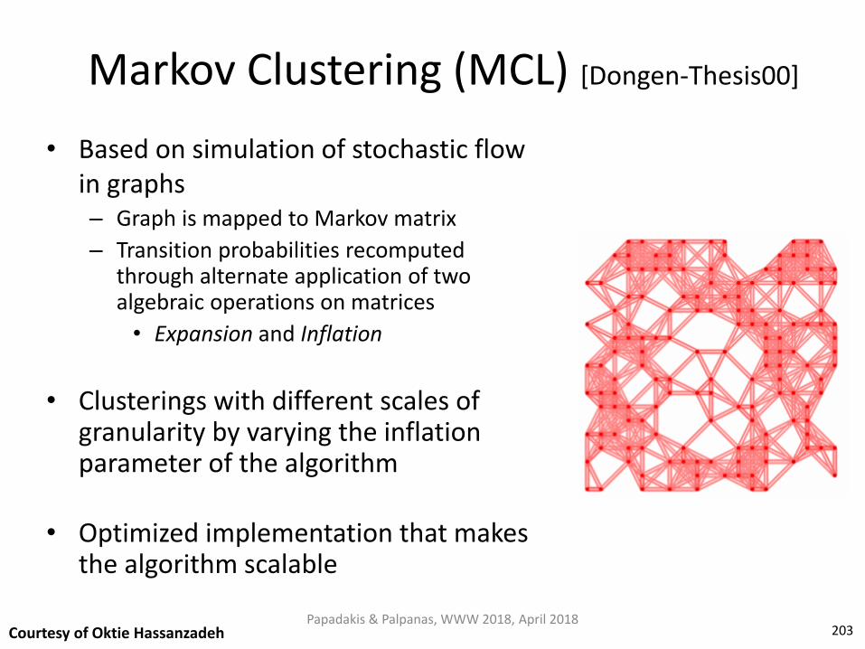
203
Markov Clustering (MCL) [Dongen-Thesis00]
• Based on simulation of stochastic flow in graphs – Graph is mapped to Markov matrix
– Transition probabilities recomputed through alternate application of two algebraic operations on matrices
• Expansion and Inflation
• Clusterings with different scales of granularity by varying the inflation parameter of the algorithm
• Optimized implementation that makes the algorithm scalable
Papadakis & Palpanas, WWW 2018, April 2018 Courtesy of Oktie Hassanzadeh 203
204
Correlation Clustering [BBC-ML04]
• Original problem: a graph clustering given edges labelled with ‘+’ or ‘−’ – ‘+’ indicates correlation between the nodes
– ‘−’ indicates uncorrelated nodes
• The goal is to find a clustering that agrees as much as possible with the edge labels – NP-Hard: approximations needed
• The labels can be assigned to edges based on the similarity scores of the records (edge weights) and a threshold value
• Several approximations exist – We use algorithm Cautious from [BBC-ML04] in our paper
Papadakis & Palpanas, WWW 2018, April 2018 Courtesy of Oktie Hassanzadeh 204

Summary of Experimental Results [Hassanzadeh et al., VLDB 2009]
Papadakis & Palpanas, WWW 2018, April 2018 205
Courtesy of Oktie Hassanzadeh

Main Conclusions [Hassanzadeh et al., VLDB 2009]
• None of the clustering algorithms produces perfect clustering • Transitive closure:
– highly scalable, but results in poor quality of duplicate groups – Poor quality even wrt other single-pass algorithms
• Most algorithms are robust to distribution of duplicates, except Ricochet algorithms: – high performance over uniformly distributed duplicates – poor performance otherwise
• Cut clustering and Correlation clustering: – sophisticated & popular algorithms – achieve lower accuracy than some single-pass algorithms
• Markov clustering: – very efficient – one the most accurate algorithms
Papadakis & Palpanas, WWW 2018, April 2018 206
Courtesy of Oktie Hassanzadeh

Papadakis & Palpanas, WWW 2018, April 2018
Part 8:
Massive Parallelization Methods
207

Massive Parallelization Outline
• Based on the Map-Reduce paradigm – Data partitioned across the nodes of a cluster
– Map Phase: transforms a data partition into (key, value) pairs
– Reduce Phase: processes pairs with the same key
• Parallelization of Blocking – Standard Blocking (Dedoop)
• Parallelization of Block Processing – Block Filtering
– Meta-blocking
• Parallelization of Entity Matching – LINDA
Papadakis & Palpanas, WWW 2018, April 2018 208

Papadakis & Palpanas, WWW 2018, April 2018 209
1: Input Key: id of entity ei, 𝑖 Value: entity profile of ei
2: Output Key: blocking key value, 𝑏𝑘𝑣 Value: entity profile of ei
3: 𝑏𝑘𝑣 = extractBlockingKey(ei) 4: emit( 𝑏𝑘𝑣 , 𝑘. ||𝑏𝑘|| );
1: Input Key: blocking key value, 𝑏𝑘𝑣 Value: list of entity profiles 𝑉 = {𝑒𝑖 , 𝑒𝑗 , … , }
2: Output Key: pair of concatenated entity ids, 𝑖. 𝑗 Value: true (match) or false (non-match)
3: for each pair of entities ei-ej in 𝑉 4: decision = compareProfiles( ei
, ej )
5: emit( 𝑖. 𝑗 , decision ); 6: end loop
MAP function pseudo-code REDUCE function pseudo-code
Parallel Standard Blocking [Kolb et al., PVLDB 2012]
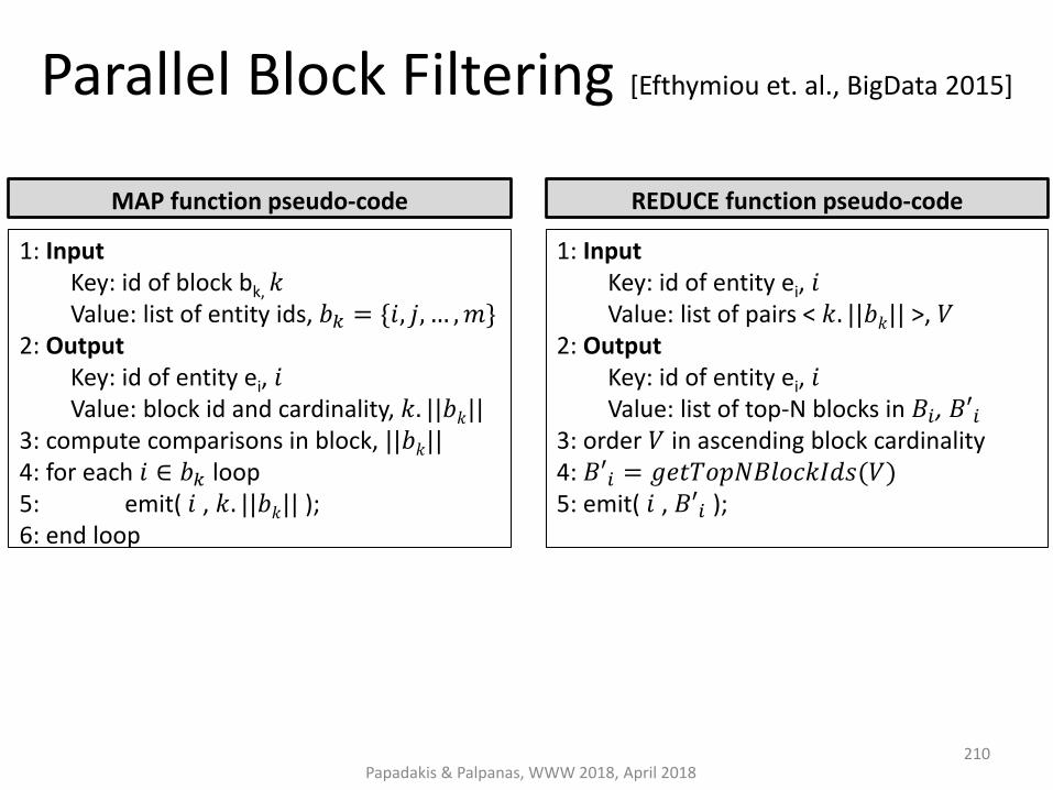
Parallel Block Filtering [Efthymiou et. al., BigData 2015]
Papadakis & Palpanas, WWW 2018, April 2018 210
1: Input Key: id of block bk, 𝑘 Value: list of entity ids, 𝑏𝑘 = {𝑖, 𝑗, … ,𝑚}
2: Output Key: id of entity ei, 𝑖 Value: block id and cardinality, 𝑘. ||𝑏𝑘||
3: compute comparisons in block, ||𝑏𝑘|| 4: for each 𝑖 ∈ 𝑏𝑘 loop 5: emit( 𝑖 , 𝑘. ||𝑏𝑘|| ); 6: end loop
1: Input Key: id of entity ei, 𝑖 Value: list of pairs < 𝑘. ||𝑏𝑘|| >, 𝑉
2: Output Key: id of entity ei, 𝑖 Value: list of top-N blocks in 𝐵𝑖, 𝐵′𝑖
3: order 𝑉 in ascending block cardinality 4: 𝐵′𝑖 = 𝑔𝑒𝑡𝑇𝑜𝑝𝑁𝐵𝑙𝑜𝑐𝑘𝐼𝑑𝑠(𝑉) 5: emit( 𝑖 , 𝐵′𝑖 );
MAP function pseudo-code REDUCE function pseudo-code

Example Parallel Block Filtering
Papadakis & Palpanas, WWW 2018, April 2018 211
b1 e1,e2,e3 … …
b4 e1,e3,e4
... ...
b6 e1,e6,e7,e9
b7 e1,e5,e6,e8,e9
... ...
Key Value
e1 b1.3
e2 b1.3
e3 b1.3 ... …
Value
e1 b4.3
e3 b4.3
e4 b4.3 ... …
Key
e1 b6.6
e6 b6.6
e7 b6.6
e9 b6.6
e1 b7.10 ... …
Map
M
ap
Gro
up
by key
e1 b1.3
e1 b4.3
e1 b6.6
e1 b7.10 ... …
Value
e2 b1.3 ... …
Key
e3 b1.3
e3 b4.3 ... …
e1 b1,b4,b6
... …
Re
du
ce
e2 b1
... …
e3 b1,b4
... …
Re
du
ce
Re
du
ce M
ap

Parallel Meta-blocking [Efthymiou et al., IS 2017]
• Three strategies:
1. Edge-based: explicitly creates the blocking graph
• needs pre-processing to perform all weight computations
• stores all edges of the blocking graph on disk
• at least 2 MapReduce jobs per pruning algorithm with high I/O
2. Comparison-based: implicitly creates the blocking graph
• defers weight computations to avoid creating any edges
• pre-processing enriches the input blocks with the block list of every entity, which is necessary for weight estimation → ideal for CEP/WEP
3. Entity-based: uses the blocking graph only as a conceptual model
• no pre-processing, all computations in the reducer
• gathers entire blocks for each entity → ideal for CNP/WNP
Papadakis & Palpanas, WWW 2018, April 2018 212
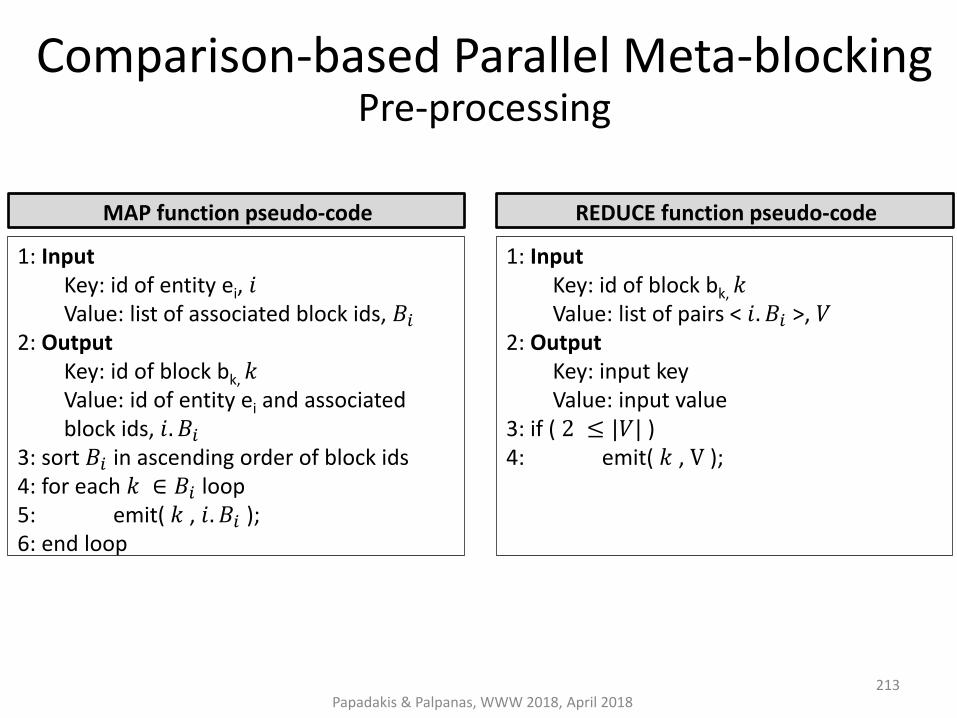
Papadakis & Palpanas, WWW 2018, April 2018 213
1: Input Key: id of entity ei, 𝑖 Value: list of associated block ids, 𝐵𝑖
2: Output Key: id of block bk, 𝑘 Value: id of entity ei and associated block ids, 𝑖. 𝐵𝑖
3: sort 𝐵𝑖 in ascending order of block ids 4: for each 𝑘 ∈ 𝐵𝑖 loop 5: emit( 𝑘 , 𝑖. 𝐵𝑖 ); 6: end loop
1: Input Key: id of block bk, 𝑘 Value: list of pairs < 𝑖. 𝐵𝑖 >, 𝑉
2: Output Key: input key Value: input value
3: if ( 2 ≤ |𝑉| ) 4: emit( 𝑘 , V );
MAP function pseudo-code REDUCE function pseudo-code
Comparison-based Parallel Meta-blocking Pre-processing

Comparison-based Parallel Meta-blocking Pre-processing Example
b1
[e1,b1,b4,b6], [e2,b1], [e3,b1,b4],...
… …
Key Value
b4
[e1,b1,b4,b6], [e3,b1,b4], [e4,b4,b5],...
... ... G
rou
p b
y key
Map
M
ap
e1 b1,b4,b6
e2 b1
e3 b1,b4
e4 b4,b5
... ...
Key Value
b1 [e1,b1,b4,b6]
b4 [e1,b1,b4,b6]
b6 [e1,b1,b4,b6]
b1 [e2,b1] ... …
Value
b1 [e3,b1,b4]
b4 [e3,b1,b4]
b4 [e4,b4,b5]
b5 [e4,b4,b5] ... …
Key Key Value
b1 [e1,b1,b4,b6]
b1 [e2,b1]
b1 [e3,b1,b4] ... …
b4 [e1,b1,b4,b6]
b4 [e3,b1,b4]
b4 [e4,b4,b5] ... …
b5 [e4,b4,b5],...
... ...
Re
du
ce
b5 [e4,b4,b5] ... …
Re
du
ce
Re
du
ce
b6 [e1,b1,b4,b6],...
... ...
Re
du
ce
b6 [e1,b1,b4,b6] ... …
Papadakis & Palpanas, WWW 2018, April 2018 214

Comparison-based Parallel Meta-blocking Weighted Edge Pruning (WEP) & Jaccard Scheme (JS)
Papadakis & Palpanas, WWW 2018, April 2018 215
MAP function pseudo-code
1: Input Key: id of block bk, 𝑘 Value: list of entity ids, associated blocks and local information, 𝑉 = {𝑖. 𝐵𝑖 . 𝑋𝑖 , 𝑗. 𝐵𝑗 . 𝑋𝑗 , … }
2: Output Key: entity ids defining edge <ni,nj>, 𝑖. 𝑗 Value: total weight of <ni,nj>, 𝑤𝑖𝑗
3: for each 𝑐𝑖𝑗 ∈ 𝑏𝑘 . 𝑐𝑜𝑚𝑝𝑎𝑟𝑖𝑠𝑜𝑛𝑠() loop
4: if ( 𝑖𝑠𝑁𝑜𝑛𝑅𝑒𝑑𝑢𝑛𝑑𝑎𝑛𝑡 𝑐𝑖𝑗 = true )
5: compute 𝑤𝑖𝑗 from 𝐵𝑖 . 𝑋𝑖, 𝐵𝑗 . 𝑋𝑗 ;
6: emit( 𝑖 . 𝑗, 𝑤𝑖𝑗 ); 7: |𝐸𝐺|++; 8: 𝑡𝑤 += 𝑤𝑖𝑗 ; 9: end loop
1: Input Key: entity ids defining edge <ni,nj>, 𝑖. 𝑗 Value: total weight of <ni,nj>, 𝑤𝑖𝑗
2: Output Key: entity ids of retained edge
<ni,nj>, 𝑖. 𝑗 Value: total weight of <ni,nj>, 𝑤𝑖𝑗
3: if ( 𝑤𝑖𝑗 > tw/ 𝐸𝐺 ) 4: emit( 𝑖. 𝑗, 𝑤𝑖𝑗 );
REDUCE function pseudo-code
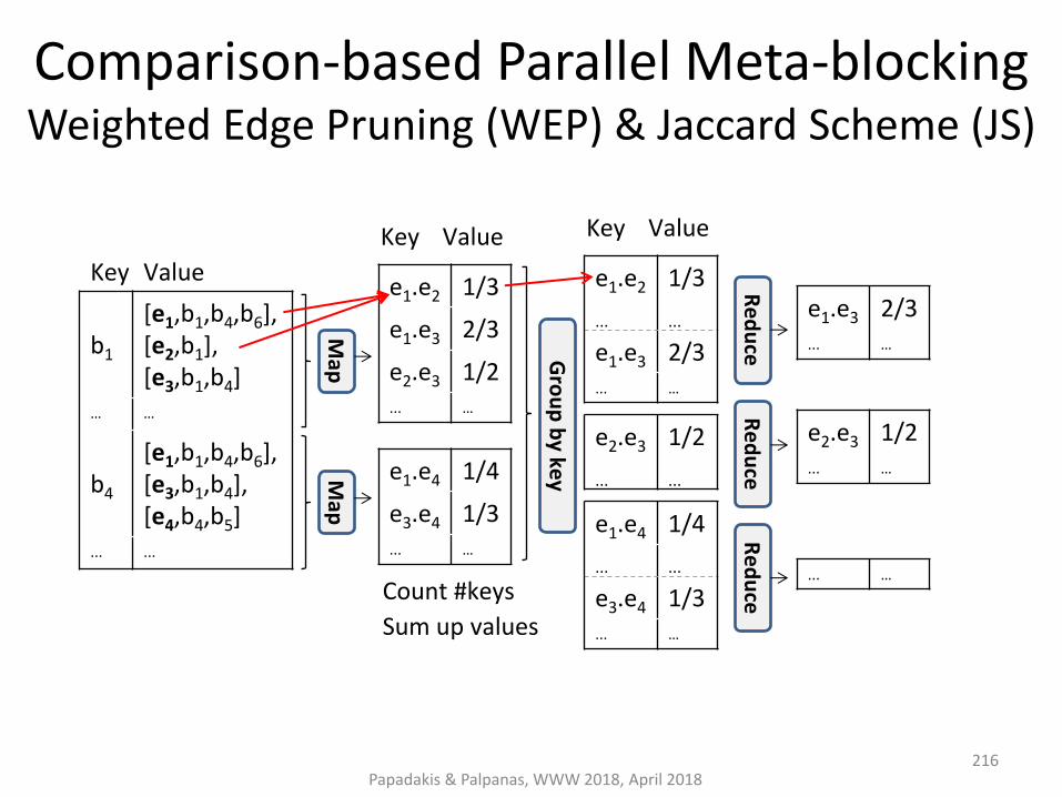
Comparison-based Parallel Meta-blocking Weighted Edge Pruning (WEP) & Jaccard Scheme (JS)
e1.e2 1/3
e1.e3 2/3
e2.e3 1/2
... …
Key Value
Gro
up
by ke
y
Re
du
ce
e1.e4 1/4
e3.e4 1/3
... …
Count #keys
Sum up values
e1.e2 1/3
... ...
e1.e3 2/3
... …
Key Value
e1.e4 1/4
... ...
e3.e4 1/3
... …
e2.e3 1/2
... ...
e1.e3 2/3
... …
e2.e3 1/2
... …
... …
Re
du
ce
Re
du
ce
b1
[e1,b1,b4,b6], [e2,b1], [e3,b1,b4]
… …
b4
[e1,b1,b4,b6], [e3,b1,b4], [e4,b4,b5]
... ...
Key Value
Map
M
ap
Papadakis & Palpanas, WWW 2018, April 2018 216
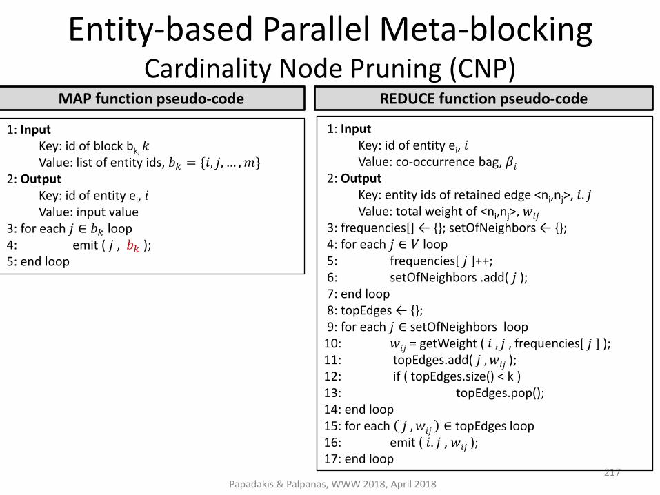
Entity-based Parallel Meta-blocking Cardinality Node Pruning (CNP)
Papadakis & Palpanas, WWW 2018, April 2018 217
1: Input Key: id of block bk, 𝑘 Value: list of entity ids, 𝑏𝑘 = {𝑖, 𝑗, … ,𝑚}
2: Output Key: id of entity ei, 𝑖 Value: input value
3: for each 𝑗 ∈ 𝑏𝑘 loop 4: emit ( 𝑗 , 𝑏𝑘 ); 5: end loop
MAP function pseudo-code REDUCE function pseudo-code
1: Input Key: id of entity ei, 𝑖 Value: co-occurrence bag, 𝛽𝑖
2: Output Key: entity ids of retained edge <ni,nj>, 𝑖. 𝑗 Value: total weight of <ni,nj>, 𝑤𝑖𝑗
3: frequencies[] ← {}; setOfNeighbors ← {}; 4: for each 𝑗 ∈ 𝑉 loop 5: frequencies[ 𝑗 ]++; 6: setOfNeighbors .add( 𝑗 ); 7: end loop 8: topEdges ← {}; 9: for each 𝑗 ∈ setOfNeighbors loop 10: 𝑤𝑖𝑗 = getWeight ( 𝑖 , 𝑗 , frequencies[ 𝑗 ] ); 11: topEdges.add( 𝑗 , 𝑤𝑖𝑗 ); 12: if ( topEdges.size() < k ) 13: topEdges.pop(); 14: end loop 15: for each 𝑗 , 𝑤𝑖𝑗 ∈ topEdges loop 16: emit ( 𝑖. 𝑗 , 𝑤𝑖𝑗 ); 17: end loop
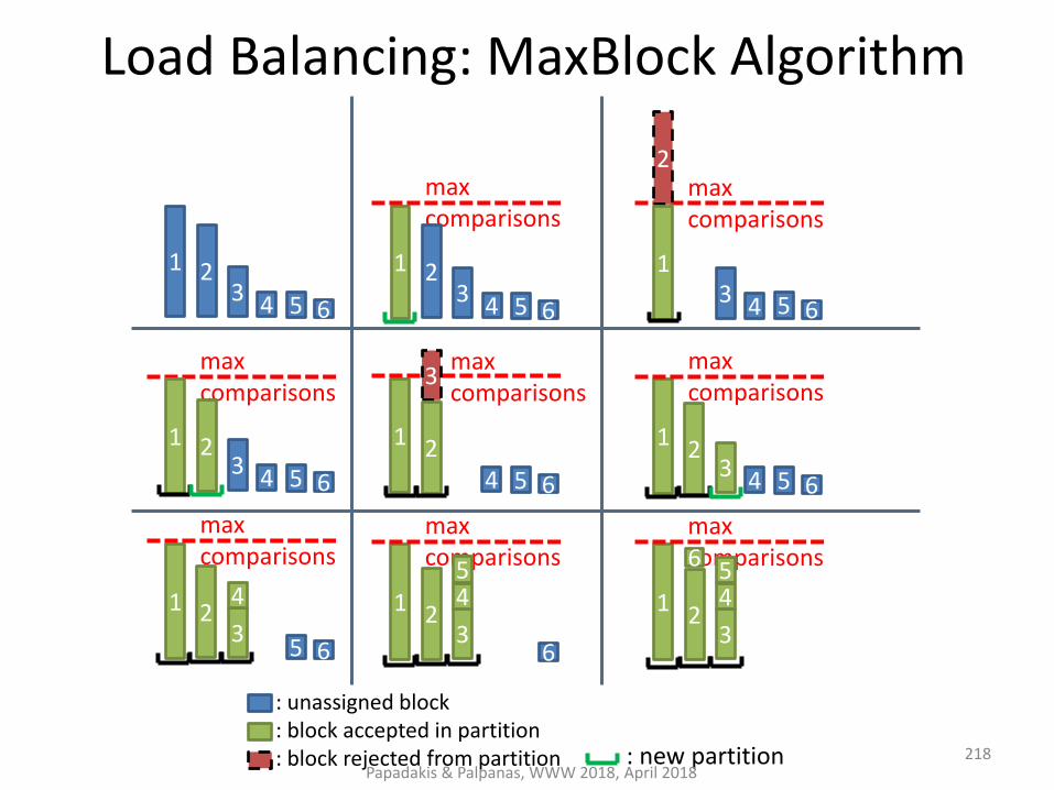
Load Balancing: MaxBlock Algorithm
1 2 3 4 5 6
1
max comparisons
2 3 4 5 6
max comparisons
3 4 5 6
max comparisons
3 4 5 6
1
max comparisons
3
4 5 6
1
max comparisons
3 4 5 6
1
max comparisons
3
4
5 6
1
max comparisons
3
4 5
6
1
max comparisons
3
4 5 6
2
2 2 2
2 2 2
1
1
: unassigned block : block accepted in partition : block rejected from partition : new partition 218
Papadakis & Palpanas, WWW 2018, April 2018
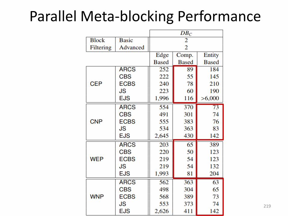
Parallel Meta-blocking Performance
Papadakis & Palpanas, WWW 2018, April 2018 219

Comparison-based Parallel Meta-blocking Weighted Edge Pruning (WEP) & Jaccard Scheme (JS)
Papadakis & Palpanas, WWW 2018, April 2018
Parallel Meta-blocking achieves (almost) linear scale-up
220
linear
parallel meta-blocking

LINDA: Parallel Entity Matching as an Optimization Problem [Böhm et al., CIKM 2012]
• Input: – Entity Graph G=(V,E) where vertices represent distinct URIs
• Output: – Assignment Matrix X where xa,b=1 if a and b refer to same entity
• Constraints: – reflexivity, symmetry, transitivity, and unique mapping per source
(entity from source 1 matches with at most one entity from source 2)
• Objective: – Given sim(a, b, G, X), find X that maximizes
Papadakis & Palpanas, WWW 2018, April 2018 221 Courtesy of Gerhard Weikum

Multi-Core Assignment Algorithm
• Initialize matrix X as identity matrix
• Initialize priority queue Q with initial similarities
• While Q not empty • Retrieve pair (a,b) of entities with highest similarity value
• Accept pairs (a’,b’) with a’ and b’ in equivalence class of a and b (uses current X to determine equivalents, updates X)
• For all pairs (c,d) of entities where similarity could have changed
• Compute new similarities in parallel
• If similarity has changed for (c,d)
• Update queue with new similarity for (c,d)
• Return X
Papadakis & Palpanas, WWW 2018, April 2018 222 Courtesy of Gerhard Weikum

Map/Reduce Assignment Algorithm
Papadakis & Palpanas, WWW 2018, April 2018
… … … … …
Queue
ei
ej
ek
el
Entity Graph
dis
trib
ute
dis
trib
ute
223
ei ej y
ei ek y
ek el y
Courtesy of Gerhard Weikum

Map/Reduce Assignment Algorithm
… … … … …
…
…
…
ei ej
…
ek el
Queue
ei
ej
ek
el
Entity Graph Q-part 1
…
…
Q-part n
dis
trib
ute
dis
trib
ute
G-part 1 G-part n
ei ej y
ei ek y
ek el y
ek el y ei ej y
Papadakis & Palpanas, WWW 2018, April 2018 224 Courtesy of Gerhard Weikum

e1 … em
e m…
e1
ei ej y
ei ek y
ek el y
… … … … …
…
ei ej y …
…
ei ej
…
ek el
Queue
Result Matrix
ei
ej
ek
el
(3) update
Entity Graph
read
read
Q-part 1
ek el y …
…
Q-part n (2) notify*
ei ej y‘
ei ek y‘ …
Queue Updates
dis
trib
ute
dis
trib
ute
dis
trib
ute
G-part 1 G-part n
Map/Reduce Assignment Algorithm
Papadakis & Palpanas, WWW 2018, April 2018 225 Courtesy of Gerhard Weikum

Papadakis & Palpanas, WWW 2018, April 2018
Part 9:
Progressive Entity Resolution
226
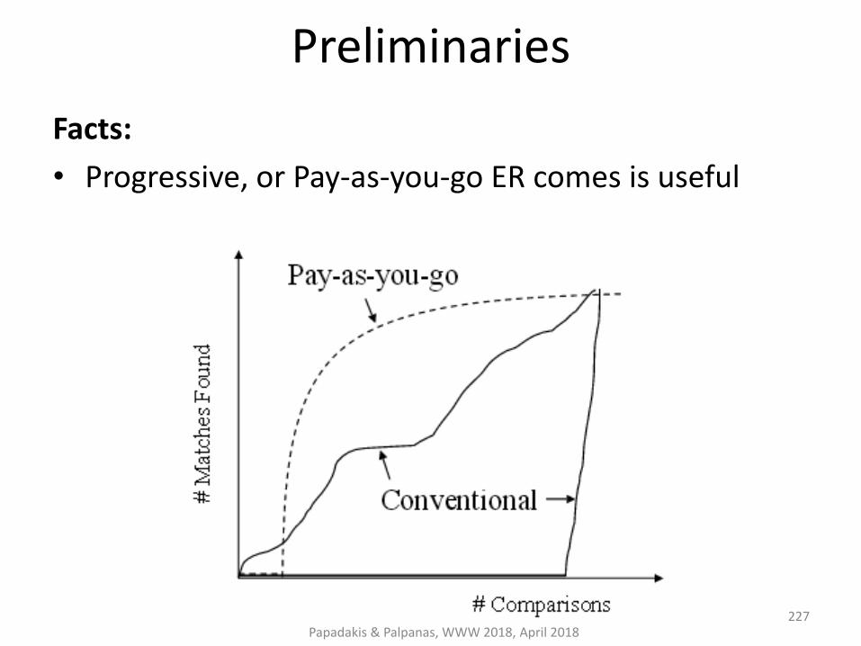
Papadakis & Palpanas, WWW 2018, April 2018
Preliminaries
Facts:
• Progressive, or Pay-as-you-go ER comes is useful
227

Papadakis & Palpanas, WWW 2018, April 2018
Preliminaries
Facts:
• Progressive, or Pay-as-you-go ER comes is useful
get most of the benefit much earlier
228
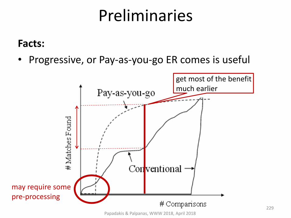
Papadakis & Palpanas, WWW 2018, April 2018
Preliminaries
Facts:
• Progressive, or Pay-as-you-go ER comes is useful
get most of the benefit much earlier
may require some pre-processing
229

Progressive Entity Resolution
• requires: – Improved Early Quality
– Same Eventual Quality
• defines optimal processing order for a set of entities
• Use cases: – Limited, unknown time for ER (online ER)
– Exploratory ER
• Empirical by nature, based on heuristics
Papadakis & Palpanas, WWW 2018, April 2018 230

Static Progressive Methods
• Guide which records to compare first, independently of Entity Matching results
• Three flavors – Sorted list of pairs: a list of record pairs, ranked by the likelihood that the
pairs match
– Hierarchy of partitions: likely matching records in the form of partitions with different levels of granularity
– Sorted list of records: maximize the number of matching records identified when the list is resolved sequentially
Papadakis & Palpanas, WWW 2018, April 2018 Courtesy of Steven Euijong Whang 231

Sorted Neighborhood
(SN)
Standard Blocking
Suffix Arrays Blocking
(SAB)
Progressive SN (PSN)
Schema-Agnostic PSN (SA-PSN)
Meta-blocking (Blocking Graph)
Ordered List of Records (OLR)
Hierarchy of Record Partitions (HRP)
Local SA-PSN (LS-PSN)
Global SA-PSN (GS-PSN)
Progressive Block Scheduling (PBS)
Progressive Suffix Arrays Blocking
(SA-PSAB)
Token Blocking
Progressive Profile Scheduling (PPS)
Batch
P
rogressive
Sch
ema-
bas
ed
Naï
ve
Ad
van
ced
Sch
ema-
agn
ost
ic
Comparison-based Block-based Profile-based Hybrid
Taxonomy of Progressive Methods
Papadakis & Palpanas, WWW 2018, April 2018 232

Progressive Sorted Neighborhood (PSN) [Whang et al, IEEE TKDE, 2013]
233
A B C D E F G H I J K L M N O P
A
B
C
D
E
F
G
H
I
J
K
L
M
N
O
P
The Comparison Matrix
Record
Comparison
Duplicate
10
6 3 1 0
Courtesy of Thorsten Papenbrock Papadakis & Palpanas, WWW 2018, April 2018

Sorted Neighborhood
(SN)
Standard Blocking
Suffix Arrays Blocking
(SAB)
Progressive SN (PSN)
Schema-Agnostic PSN (SA-PSN)
Meta-blocking (Blocking Graph)
Ordered List of Records (OLR)
Hierarchy of Record Partitions (HRP)
Local SA-PSN (LS-PSN)
Global SA-PSN (GS-PSN)
Progressive Block Scheduling (PBS)
Progressive Suffix Arrays Blocking
(SA-PSAB)
Token Blocking
Progressive Profile Scheduling (PPS)
Batch
P
rogressive
Sch
ema-
bas
ed
Naï
ve
Ad
van
ced
Sch
ema-
agn
ost
ic
Comparison-based Block-based Profile-based Hybrid
Taxonomy of Progressive Methods
Papadakis & Palpanas, WWW 2018, April 2018 234

Hierarchy of Partitions [Whang et al, IEEE TKDE, 2013]
1. Compare {r1, r2} and {r4, r5}.
2. If there is more budget, compare {r1, r2, r3}.
3. If there is still more budget, compare {r1, r2, r3, r4, r5}.
235 Courtesy of Steven Euijong Whang Papadakis & Palpanas, WWW 2018, April 2018

Sorted Neighborhood
(SN)
Standard Blocking
Suffix Arrays Blocking
(SAB)
Progressive SN (PSN)
Schema-Agnostic PSN (SA-PSN)
Meta-blocking (Blocking Graph)
Ordered List of Records (OLR)
Hierarchy of Record Partitions (HRP)
Local SA-PSN (LS-PSN)
Global SA-PSN (GS-PSN)
Progressive Block Scheduling (PBS)
Progressive Suffix Arrays Blocking
(SA-PSAB)
Token Blocking
Progressive Profile Scheduling (PPS)
Batch
P
rogressive
Sch
ema-
bas
ed
Naï
ve
Ad
van
ced
Sch
ema-
agn
ost
ic
Comparison-based Block-based Profile-based Hybrid
Taxonomy of Progressive Methods
Papadakis & Palpanas, WWW 2018, April 2018 236
Ordered List of Records [Whang et al, IEEE TKDE, 2013]
Goal: maximize the number of matching records identified while resolving the
list sequentially
Advantages: • zero space requirements
• no change in resolution algorithm
Generation: Sort all entities according to a weight derived from the partitions that involve them, under the assumption that each partition is equally likely to be the correct ER outcome.
Papadakis & Palpanas, WWW 2018, April 2018 237

Schema-agnostic Progressive ER [Simonini et. al., ICDE 2018]
• Previous works assume structured data. – (Multiple) Schema-based blocking methods.
• Problems: – Inapplicable to Big Data, due to Volume and Variety.
– Plenty of room for improvement
• even for schema-based methods!
Papadakis & Palpanas, WWW 2018, April 2018 238

Schema-agnostic Progressive ER [Simonini et. al., ICDE 2018]
• state of the art schema-based solution: PSN
Papadakis & Palpanas, WWW 2018, April 2018 239

Schema-agnostic Progressive ER [Simonini et. al., ICDE 2018]
• state of the art schema-based solution: PSN
• when optimal finds 100% of matches, PSN finds 2-35% of matches
Papadakis & Palpanas, WWW 2018, April 2018 240

Schema-agnostic Progressive ER [Simonini et. al., ICDE 2018]
• state of the art schema-based solution: PSN
• when optimal finds 100% of matches, PSN finds 2-35% of matches
• after 10x the comparisons optimal needs, PSN finds 15-85% of matches
Papadakis & Palpanas, WWW 2018, April 2018 241

Schema-agnostic Progressive ER [Simonini et. al., ICDE 2018]
• state of the art schema-based solution: PSN
• when optimal finds 100% of matches, PSN finds 2-35% of matches
• after 10x the comparisons optimal needs, PSN finds 15-85% of matches
• after 100x the comparisons optimal needs, PSN finds 80-99% of matches
Papadakis & Palpanas, WWW 2018, April 2018 242

Schema-agnostic Progressive ER [Simonini et. al., ICDE 2018]
• Solution: – schema-agnostic methods that are able to handle large, semi-structured,
heterogeneous data
– proposed solutions also applicable to structured data
Papadakis & Palpanas, WWW 2018, April 2018 243

Sorted Neighborhood
(SN)
Standard Blocking
Suffix Arrays Blocking
(SAB)
Progressive SN (PSN)
Schema-Agnostic PSN (SA-PSN)
Meta-blocking (Blocking Graph)
Ordered List of Records (OLR)
Hierarchy of Record Partitions (HRP)
Local SA-PSN (LS-PSN)
Global SA-PSN (GS-PSN)
Progressive Block Scheduling (PBS)
Progressive Suffix Arrays Blocking
(SA-PSAB)
Token Blocking
Progressive Profile Scheduling (PPS)
Batch
P
rogressive
Sch
ema-
bas
ed
Naï
ve
Ad
van
ced
Sch
ema-
agn
ost
ic
Comparison-based Block-based Profile-based Hybrid
Taxonomy of Progressive Methods
Papadakis & Palpanas, WWW 2018, April 2018 244

Schema-agnostic PSN [Simonini et. al., ICDE 2018]
• Use all attribute values as blocking keys – regardless of attribute values
• Sort them alphabetically
• Sort the entities accordingly → Neighbor List – The same entity might be placed in consecutive places
• Slide the incremental window over the Neighbor List
• Execute the valid comparisons
Papadakis & Palpanas, WWW 2018, April 2018 245

Example of Schema-agnostic PSN
Papadakis & Palpanas, WWW 2018, April 2018
Data Lake
Blocking Keys
Neighbor List
Sliding Window
246

Sorted Neighborhood
(SN)
Standard Blocking
Suffix Arrays Blocking
(SAB)
Progressive SN (PSN)
Schema-Agnostic PSN (SA-PSN)
Meta-blocking (Blocking Graph)
Ordered List of Records (OLR)
Hierarchy of Record Partitions (HRP)
Local SA-PSN (LS-PSN)
Global SA-PSN (GS-PSN)
Progressive Block Scheduling (PBS)
Progressive Suffix Arrays Blocking
(SA-PSAB)
Token Blocking
Progressive Profile Scheduling (PPS)
Batch
P
rogressive
Sch
ema-
bas
ed
Naï
ve
Ad
van
ced
Sch
ema-
agn
ost
ic
Comparison-based Block-based Profile-based Hybrid
Taxonomy of Progressive Methods
Papadakis & Palpanas, WWW 2018, April 2018 247
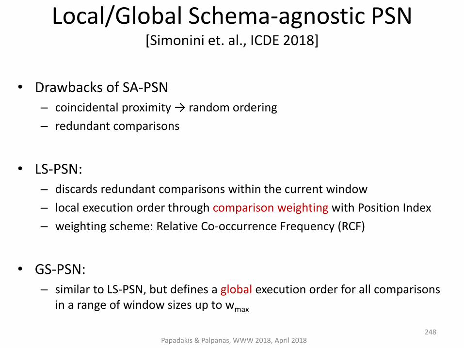
Local/Global Schema-agnostic PSN [Simonini et. al., ICDE 2018]
• Drawbacks of SA-PSN – coincidental proximity → random ordering
– redundant comparisons
• LS-PSN: – discards redundant comparisons within the current window
– local execution order through comparison weighting with Position Index
– weighting scheme: Relative Co-occurrence Frequency (RCF)
• GS-PSN: – similar to LS-PSN, but defines a global execution order for all comparisons
in a range of window sizes up to wmax
Papadakis & Palpanas, WWW 2018, April 2018 248

Example of LS-PSN
Papadakis & Palpanas, WWW 2018, April 2018
Data Lake
Blocking Keys
Neighbor List
Sliding Window
Comparison Sorting
Comparison Weighting
249

Sorted Neighborhood
(SN)
Standard Blocking
Suffix Arrays Blocking
(SAB)
Progressive SN (PSN)
Schema-Agnostic PSN (SA-PSN)
Meta-blocking (Blocking Graph)
Ordered List of Records (OLR)
Hierarchy of Record Partitions (HRP)
Local SA-PSN (LS-PSN)
Global SA-PSN (GS-PSN)
Progressive Block Scheduling (PBS)
Progressive Suffix Arrays Blocking
(SA-PSAB)
Token Blocking
Progressive Profile Scheduling (PPS)
Batch
P
rogressive
Sch
ema-
bas
ed
Naï
ve
Ad
van
ced
Sch
ema-
agn
ost
ic
Comparison-based Block-based Profile-based Hybrid
Taxonomy of Progressive Methods
Papadakis & Palpanas, WWW 2018, April 2018 250

Progressive Suffix Arrays Blocking [Simonini et. al., ICDE 2018]
• Every token in any attribute value is a blocking key
• Every key is converted to all suffixes with at least lmin characters
• Every suffix of minimum length creates a tree with that suffix at its root → Hierarchy of Partitions
Papadakis & Palpanas, WWW 2018, April 2018 251

Sorted Neighborhood
(SN)
Standard Blocking
Suffix Arrays Blocking
(SAB)
Progressive SN (PSN)
Schema-Agnostic PSN (SA-PSN)
Meta-blocking (Blocking Graph)
Ordered List of Records (OLR)
Hierarchy of Record Partitions (HRP)
Local SA-PSN (LS-PSN)
Global SA-PSN (GS-PSN)
Progressive Block Scheduling (PBS)
Progressive Suffix Arrays Blocking
(SA-PSAB)
Token Blocking
Progressive Profile Scheduling (PPS)
Batch
P
rogressive
Sch
ema-
bas
ed
Naï
ve
Ad
van
ced
Sch
ema-
agn
ost
ic
Comparison-based Block-based Profile-based Hybrid
Taxonomy of Progressive Methods
Papadakis & Palpanas, WWW 2018, April 2018 252

Progressive Block Scheduling (PBS) [Simonini et. al., ICDE 2018]
• Based on redundancy-positive blocking methods
• Orders blocks in increasing comparisons
• For each block: – Estimate the weight of all comparisons
– Sort and process the non-redundant comparisons in decreasing weight
– Relies on Entity (Profile) Index
Papadakis & Palpanas, WWW 2018, April 2018 253

Example of PBS
Papadakis & Palpanas, WWW 2018, April 2018
Data Lake
Block Collection
Block Processing
254

Sorted Neighborhood
(SN)
Standard Blocking
Suffix Arrays Blocking
(SAB)
Progressive SN (PSN)
Schema-Agnostic PSN (SA-PSN)
Meta-blocking (Blocking Graph)
Ordered List of Records (OLR)
Hierarchy of Record Partitions (HRP)
Local SA-PSN (LS-PSN)
Global SA-PSN (GS-PSN)
Progressive Block Scheduling (PBS)
Progressive Suffix Arrays Blocking
(SA-PSAB)
Token Blocking
Progressive Profile Scheduling (PPS)
Batch
P
rogressive
Sch
ema-
bas
ed
Naï
ve
Ad
van
ced
Sch
ema-
agn
ost
ic
Comparison-based Block-based Profile-based Hybrid
Taxonomy of Progressive Methods
Papadakis & Palpanas, WWW 2018, April 2018 255

Progressive Profile Scheduling (PPS) [Simonini et. al., ICDE 2018]
• Based on redundancy-positive blocking methods
• Orders entities in decreasing duplication likelihood
• Simultaneously, it aggregates the top-weighted comparison per entity → these are the first comparisons to be processed
• Processes one entity at a time – For each entity, it considers the k top-weighted co-occurring ones in
decreasing edge weight
Papadakis & Palpanas, WWW 2018, April 2018 256

Example of PPS
Papadakis & Palpanas, WWW 2018, April 2018
Data Lake
Block Collection
Blocking Graph
Sorted Profile List
Local Comparison List for p2
257

Experimental Results [Simonini et. al., ICDE 2018]
• datasets used:
Papadakis & Palpanas, WWW 2018, April 2018 258

Experimental Results [Simonini et. al., ICDE 2018]
• datasets used:
Papadakis & Palpanas, WWW 2018, April 2018 259
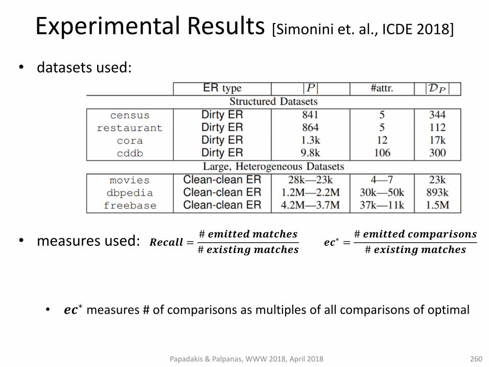
Experimental Results [Simonini et. al., ICDE 2018]
• datasets used:
• measures used: 𝑹𝒆𝒄𝒂𝒍𝒍 =# 𝒆𝒎𝒊𝒕𝒕𝒆𝒅 𝒎𝒂𝒕𝒄𝒉𝒆𝒔
# 𝒆𝒙𝒊𝒔𝒕𝒊𝒏𝒈 𝒎𝒂𝒕𝒄𝒉𝒆𝒔 𝒆𝒄∗ =
# 𝒆𝒎𝒊𝒕𝒕𝒆𝒅 𝒄𝒐𝒎𝒑𝒂𝒓𝒊𝒔𝒐𝒏𝒔
# 𝒆𝒙𝒊𝒔𝒕𝒊𝒏𝒈 𝒎𝒂𝒕𝒄𝒉𝒆𝒔
• 𝒆𝒄∗ measures # of comparisons as multiples of all comparisons of optimal
Papadakis & Palpanas, WWW 2018, April 2018 260

Experimental Results [Simonini et. al., ICDE 2018]
• datasets used:
• measures used: 𝑹𝒆𝒄𝒂𝒍𝒍 =# 𝒆𝒎𝒊𝒕𝒕𝒆𝒅 𝒎𝒂𝒕𝒄𝒉𝒆𝒔
# 𝒆𝒙𝒊𝒔𝒕𝒊𝒏𝒈 𝒎𝒂𝒕𝒄𝒉𝒆𝒔
𝒂𝒓𝒆𝒂 𝒖𝒏𝒅𝒆𝒓 𝒄𝒖𝒓𝒗𝒆: 𝑨𝑼𝑪𝒎∗ @𝒆𝒄∗ =
𝑹𝒆𝒄𝒂𝒍𝒍 𝑪𝒖𝒓𝒗𝒆 𝒐𝒇 𝒎
𝒊𝒅𝒆𝒂𝒍 𝑹𝒆𝒄𝒂𝒍𝒍 𝑪𝒖𝒓𝒗𝒆
𝒆𝒄∗
𝟎
𝒆𝒄∗ =# 𝒆𝒎𝒊𝒕𝒕𝒆𝒅 𝒄𝒐𝒎𝒑𝒂𝒓𝒊𝒔𝒐𝒏𝒔
# 𝒆𝒙𝒊𝒔𝒕𝒊𝒏𝒈 𝒎𝒂𝒕𝒄𝒉𝒆𝒔
• 𝒆𝒄∗ measures # of comparisons as multiples of all comparisons of optimal • 𝑨𝑼𝑪𝒎
∗ @𝒆𝒄∗ measures performance of method m for effort 𝒆𝒄∗ • the higher the 𝑨𝑼𝑪𝒎
∗ @𝒆𝒄∗, the better (optimal has 𝑨𝑼𝑪𝒎∗ @𝒆𝒄∗=1)
Papadakis & Palpanas, WWW 2018, April 2018 261

Experimental Results [Simonini et. al., ICDE 2018]
Papadakis & Palpanas, WWW 2018, April 2018
• performance over heterogeneous datasets
262

Experimental Results [Simonini et. al., ICDE 2018]
Papadakis & Palpanas, WWW 2018, April 2018
• performance over heterogeneous datasets
263
• methods based on redundancy-positive blocking perform significantly better
• PPS is the winner

Experimental Results [Simonini et. al., ICDE 2018]
Papadakis & Palpanas, WWW 2018, April 2018
264
• performance over structured datasets

Experimental Results [Simonini et. al., ICDE 2018]
Papadakis & Palpanas, WWW 2018, April 2018
265
• performance over structured datasets
• the LS/GS-PSN methods perform significantly better

Experimental Results [Simonini et. al., ICDE 2018]
Papadakis & Palpanas, WWW 2018, April 2018
266
• performance over structured datasets
• the LS/GS-PSN methods perform significantly better • PPS achieves almost the same performance

Experimental Results [Simonini et. al., ICDE 2018]
Papadakis & Palpanas, WWW 2018, April 2018
267
• performance over structured datasets
• the LS/GS-PSN methods perform significantly better • PPS achieves almost the same performance
• overall, PPS is method of choice for progressive ER on both structured/ heterogeneous data

Dynamic Progressive Methods
• Problem of Static Methods: – The order of comparisons is immutable.
• Impact: – The algorithm cannot react to a skewed distribution of duplicates.
• Solution: – If (i,j) is a duplicate, then check (i+1,j) and (i,j+1) as well.
– Assumption:
• Oracle for Entity Matching
Papadakis & Palpanas, WWW 2018, April 2018 268

Dynamic Progressive SN [Papenbrock et a., IEEE TKDE, 2015]
269
Courtesy of Thorsten Papenbrock Papadakis & Palpanas, WWW 2018, April 2018

Papadakis & Palpanas, WWW 2018, April 2018
Part 10:
JedAI Toolkit
270
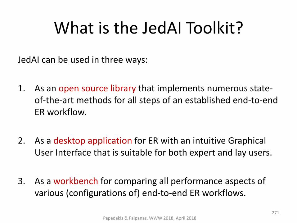
What is the JedAI Toolkit?
JedAI can be used in three ways:
1. As an open source library that implements numerous state-of-the-art methods for all steps of an established end-to-end ER workflow.
2. As a desktop application for ER with an intuitive Graphical User Interface that is suitable for both expert and lay users.
3. As a workbench for comparing all performance aspects of various (configurations of) end-to-end ER workflows.
Papadakis & Palpanas, WWW 2018, April 2018 271

JedAI vs other tools
Magellan
× limited variety of (blocking) methods
rich variety available methods for every step in the end-to-end workflow
Papadakis & Palpanas, WWW 2018, April 2018 272
JedAI

JedAI vs other tools
Magellan
× limited variety of (blocking) methods
× restricted to relational data only
rich variety available methods for every step in the end-to-end workflow
applies to both structured and non-structured data
Papadakis & Palpanas, WWW 2018, April 2018 273
JedAI

JedAI vs other tools
Magellan
× limited variety of (blocking) methods
× restricted to relational data only
× targeted to expert users, focusing on development of tailor-made methods
rich variety available methods for every step in the end-to-end workflow
applies to both structured and non-structured data
hands-off functionality through default configuration of every method, but also extensible
Papadakis & Palpanas, WWW 2018, April 2018 274
JedAI

JedAI vs other tools
Magellan
× limited variety of (blocking) methods
× restricted to relational data only
× targeted to expert users, focusing on development of tailor-made methods
× offers command-line interface, no GUI
rich variety available methods for every step in the end-to-end workflow
applies to both structured and non-structured data
hands-off functionality through default configuration of every method, but also extensible
intuitive GUI with guidelines even for novice users
Papadakis & Palpanas, WWW 2018, April 2018 275
JedAI

JedAI vs other tools
Magellan
× limited variety of (blocking) methods
× restricted to relational data only
× targeted to expert users, focusing on development of tailor-made methods
× offers command-line interface, no GUI
JedAI
rich variety available methods for every step in the end-to-end workflow
applies to both structured and non-structured data
hands-off functionality through default configuration of every method, but also extensible
intuitive GUI with guidelines even for novice users
multi-core execution (coming soon)
Papadakis & Palpanas, WWW 2018, April 2018 276

How does the JedAI Toolkit work?
JedAI implements the following schema-agnostic, end-to-end workflow for both Clean-Clean and Dirty ER:
Data Reading
Block Building
Block Cleaning
Comparison Cleaning
Entity Matching
Entity Clustering
Evaluation & Storing
Step 5 Step 2 Step 3 Step 4 Step 6 Step 1 Step 7
Reads files containing the entity
profiles and the golden standard.
Creates overlapping
blocks.
Optional step that cleans blocks from
useless comparisons
(repeated, superfluous).
Optional step that operates on
the level of individual
comparisons to remove the
useless ones.
Executes all retained
comparisons.
Partitions the similarity graph into equivalence
clusters.
Stores and presents
performance results w.r.t.
numerous measures.
Papadakis & Palpanas, WWW 2018, April 2018 277

How is the JedAI Toolkit structured?
???
Papadakis & Palpanas, WWW 2018, April 2018
• Modular architecture – one module per workflow step
• Extensible architecture – e.g., ontology matching module
278
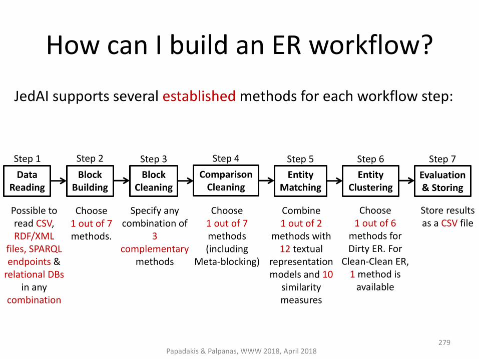
How can I build an ER workflow?
JedAI supports several established methods for each workflow step:
Data Reading
Block Building
Block Cleaning
Comparison Cleaning
Entity Matching
Entity Clustering
Evaluation & Storing
Step 5 Step 2 Step 3 Step 4 Step 6 Step 1 Step 7
Possible to read CSV, RDF/XML
files, SPARQL endpoints &
relational DBs in any
combination
Choose 1 out of 7 methods.
Specify any combination of
3 complementary
methods
Choose 1 out of 7 methods (including
Meta-blocking)
Combine 1 out of 2
methods with 12 textual
representation models and 10
similarity measures
Choose 1 out of 6
methods for Dirty ER. For
Clean-Clean ER, 1 method is
available
Store results as a CSV file
Papadakis & Palpanas, WWW 2018, April 2018 279

Which Data Formats are supported?
Papadakis & Palpanas, WWW 2018, April 2018 280
Data Formats
CSV files
Relational databases
XML/RDF/OWL files
SPARQL endpoints
Java Serialized Objects (using JedAI data model)

Which Blocking Methods are supported?
Block Building Block Cleaning Comparison Cleaning
Token Blocking Block Filtering Comparison Propagation
Sorted Neighborhood Size-based Block Purging Cardinality Edge Pruning (CEP)
Extended Sorted Neighborhood
Cardinality-based Block Purging
Cardinality Node Pruning (CNP)
Q-Grams Blocking Block Scheduling Weighted Edge Pruning (WEP)
Extended Q-Grams Blocking Weighted Node Pruning (WNP)
Suffix Arrays Reciprocal CNP
Extended Suffix Arrays Reciprocal WNP
Papadakis & Palpanas, WWW 2018, April 2018 281

Which Entity Matching/Clustering Methods are supported?
Papadakis & Palpanas, WWW 2018, April 2018 282
Entity Matching Entity Clustering
Group Linkage* Center Clustering
Profile Matcher* Connected Components
Cut Clustering
* In combination with bag and graph textual models based on token and character n-grams and various established string similarity measures
Markov Clustering
Merge-Center Clustering
Ricochet SR Clustering
Unique Mapping Clustering

Which Datasets are included?
Clean-Clean ER (real)
D1 Entities
D2 Entities
Abt-Buy 1,076 1,076
DBLP-ACM 2,616 2,294
DBLP-Scholar 2,516 61,353
Amazon-GP 1,354 3,039
Movies 27,615 23,182
DBPedia 1,190,733 2,164,040
Papadakis & Palpanas, WWW 2018, April 2018
Dirty ER (synthetic)
Entities
10K 10,000
50K 50,000
100K 100,000
200K 200,00
300K 300,00
1M 1,000,000
2M 2,000,000
can be used for Dirty ER, too
Several datasets are available for testing
283
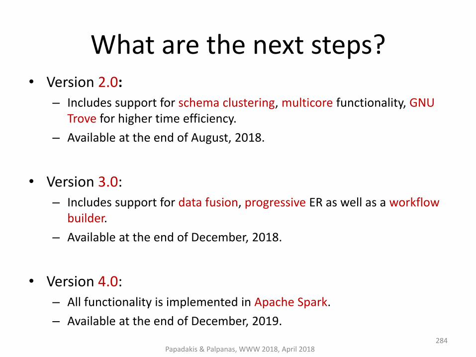
What are the next steps? • Version 2.0:
– Includes support for schema clustering, multicore functionality, GNU Trove for higher time efficiency.
– Available at the end of August, 2018.
• Version 3.0: – Includes support for data fusion, progressive ER as well as a workflow
builder.
– Available at the end of December, 2018.
• Version 4.0: – All functionality is implemented in Apache Spark.
– Available at the end of December, 2019.
Papadakis & Palpanas, WWW 2018, April 2018 284

Where can I find JedAI Toolkit? • Project website: http://jedai.scify.org
• Documentation (slides, videos, etc) available at github
• Github repositories: – JedAI Library: https://github.com/scify/JedAIToolkit
– JedAI Desktop Application and Workbench: https://github.com/scify/jedai-ui .
– All code is implemented using Java 8.
– All code is publicly available under Apache License V2.0.
Papadakis & Palpanas, WWW 2018, April 2018 285

Where can I find JedAI Toolkit? • Project website: http://jedai.scify.org
• Documentation (slides, videos, etc) available at github
• Github repositories: – JedAI Library: https://github.com/scify/JedAIToolkit
– JedAI Desktop Application and Workbench: https://github.com/scify/jedai-ui .
– All code is implemented using Java 8.
– All code is publicly available under Apache License V2.0.
• JedAI already used in the industry, and in university courses
• When using JedAI, please cite: George Papadakis, Leonidas Tsekouras, Emmanouil Thanos, George Giannakopoulos, Themis Palpanas and Manolis Koubarakis: "JedAI: The Force behind Entity Resolution", in ESWC 2017
Papadakis & Palpanas, WWW 2018, April 2018 286

Papadakis & Palpanas, WWW 2018, April 2018
Part 11:
Challenges
287

Papadakis & Palpanas, WWW 2018, April 2018
Automatic Configuration
Facts:
• Several parameters in every blocking workflow – Both for lazy and proactive methods
• Blocking performance sensitive to internal configuration – Experimentally verified in [Papadakis et. al., VLDB 2016]
• Manual fine-tuning required
Open Research Directions:
• Plug-and-play blocking
• Data-driven configuration
288

Papadakis & Palpanas, WWW 2018, April 2018
Privacy Preserving Blocking
Facts:
• several applications ask for privacy-preserving ER
• lots of interest in this area
[Christen, PADM 2006][Karakasidis et al., 2012][Ziad et al, BTW 2015]
Open Research Directions:
• What is the role of blocking workflow techniques? – block building, block filtering, comparison cleaning
• How can existing blocking techniques be adjusted?
• Novel blocking methods for this context
289

Papadakis & Palpanas, WWW 2018, April 2018
Incremental Blocking
Facts:
• Velocity in Web Data
• Dynamic ER
• Incremental ER [Gruenheid et. al., VLDB 2014] – Blocking → black box
Open Research Directions:
• Incremental (Meta-)Blocking
290

Papadakis & Palpanas, WWW 2018, April 2018
Distributed Blocking
Facts: • Velocity in Big Data
• Need for even faster/more scalable ER solutions
Open Research Directions: • What is the best way to use the modern distributed platforms/paradigms?
– Flink/Spark
• How can we further improve performance of Parallel Meta-blocking?
– Gelly/Gradoop/GraphX
• Minimize both time performance and total CPU cycles
291

Papadakis & Palpanas, WWW 2018, April 2018
Part 12:
Conclusions
292

Conclusions – Block Building
• Traditional proactive blocking methods only suitable for relational data – background schema knowledge should be available for their
configuration
• Recent lazy blocking methods scale well to heterogeneous, semi-structured Big Data – Variety is addressed with schema-agnostic keys
– Volume is addressed with Block and Comparison Cleaning methods → they trade slightly lower recall, for much higher precision
– Token Blocking → the only parameter-free blocking method
Papadakis & Palpanas, WWW 2018, April 2018 293
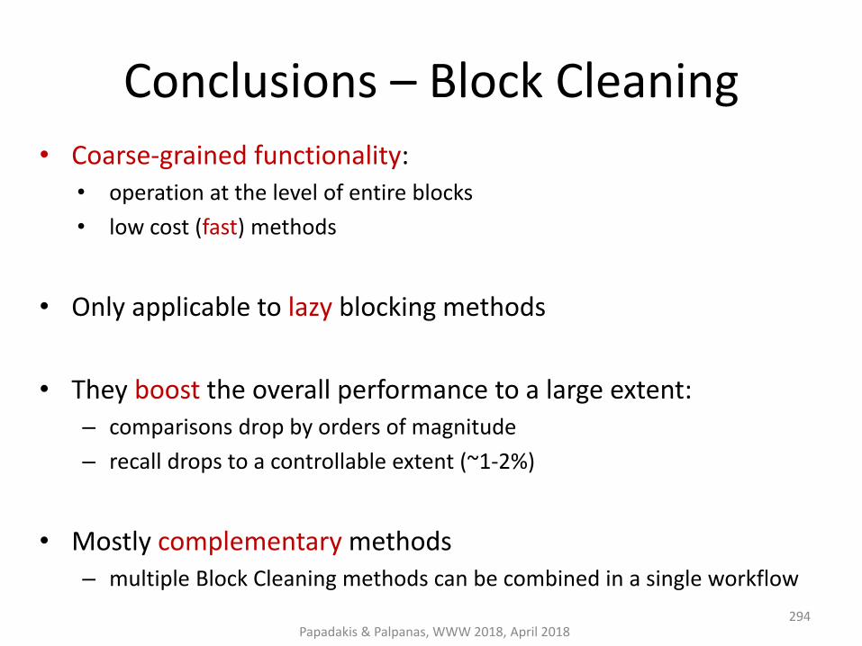
Conclusions – Block Cleaning
• Coarse-grained functionality: • operation at the level of entire blocks
• low cost (fast) methods
• Only applicable to lazy blocking methods
• They boost the overall performance to a large extent: – comparisons drop by orders of magnitude
– recall drops to a controllable extent (~1-2%)
• Mostly complementary methods – multiple Block Cleaning methods can be combined in a single workflow
Papadakis & Palpanas, WWW 2018, April 2018 294

Conclusions – Comparison Cleaning
• Fine-grained functionality: – operate at the level of individual comparisons → computationally intensive
process
• Apply to both lazy and proactive methods
• Meta-blocking is the current state-of-the-art – Discards both superfluous and redundant comparisons
– Necessary for reducing comparisons to manageable levels
• reduces comparisons by orders of magnitude, with recall > 98%
– Naturally parallelizable
Papadakis & Palpanas, WWW 2018, April 2018 295

Big Data Research (BDR) Journal http://www.journals.elsevier.com/big-data-research/
• New Elsevier journal on topics related to big data – advances in big data management/processing
– interdisciplinary applications
• Editor in Chief for BDR – submit your work
– propose special issues
• google: bdr journal
Papadakis & Palpanas, WWW 2018, April 2018 296

thank you!
questions?
http://sourceforge.net/projects/erframework
google: themis palpanas
-> publications -> tutorials
Papadakis & Palpanas, WWW 2018, April 2018 297
References – Part A [Aizawa et. al., WIRI 2005] Akiko N. Aizawa, Keizo Oyama, "A Fast Linkage Detection Scheme for Multi-Source Information Integration" in WIRI, 2005.
[Baxter et. al., KDD 2003] R. Baxter, P. Christen, T. Churches, “A comparison of fast blocking methods for record linkage”, in Workshop on Data Cleaning, Record Linkage and Object Consolidation at KDD, 2003.
[Bilenko et. al., ICDM 2006] Mikhail Bilenko, Beena Kamath, Raymond J. Mooney, "Adaptive Blocking: Learning to Scale Up Record Linkage", in ICDM 2006.
[Christen, PADM 2006] Christen P: Privacy-preserving data linkage and geocoding: Current approaches and research directions. PADM held at IEEE ICDM, Hong Kong, 2006.
[Christen, TKDE 2011] P. Christen, "A survey of indexing techniques for scalable record linkage and deduplication.” in IEEE TKDE 2011.
[Efthymiou et. al., BigData 2015] Vasilis Efthymiou, George Papadakis, George Papastefanatos, Kostas Stefanidis, Themis Palpanas, "Parallel meta-blocking: Realizing scalable entity resolution over large, heterogeneous data", in IEEE Big Data 2015.
[Fellegi et. al., JASS 1969] P. Fellegi, A. Sunter, “A theory for record linkage,” in Journal of the American Statistical Society, vol. 64, no. 328, 1969.
[Fisher et. al., KDD 2015] Jeffrey Fisher, Peter Christen, Qing Wang, Erhard Rahm, "A Clustering-Based Framework to Control Block Sizes for Entity Resolution" in KDD 2015.
[Gravano et. al., VLDB 2001] L. Gravano, P. Ipeirotis, H. Jagadish, N. Koudas, S. Muthukrishnan, D. Srivastava, “Approximate string joins in a database (almost) for free’, in VLDB, 2001.
[Gruenheid et. al., VLDB 2014] Anja Gruenheid, Xin Luna Dong, Divesh Srivastava, "Incremental Record Linkage", in PVLDB 2014.
[Hernandez et. al., SIGMOD 1995] M. Hernandez, S. Stolfo, “The merge/purge problem for large databases”, in SIGMOD, 1995.
Papadakis & Palpanas, WWW 2018, April 2018 298

References – Part B [Karakasidis et al., SAC 2012] Karakasidis A and Verykios VS: Reference table based k-anonymous private blocking. Symposium on Applied Computing, 2012.
[Kenig et. al., IS 2013] Batya Kenig, Avigdor Gal, "MFIBlocks: An effective blocking algorithm for entity resolution", in Inf. Syst. 2013.
[Ma et. Al., WSDM 2013] Y. Ma, T. Tran, "TYPiMatch: type-specific unsupervised learning of keys and key values for heterogeneous web data integration", in WSDM 2013.
[McCallum et. al., KDD 2000] A. McCallum, K. Nigam, L. Ungar, “Efficient clustering of high-dimensional data sets with application to reference matching”, in KDD, 2000.
[Michelson et. al., AAAI 2006] Matthew Michelson, Craig A. Knoblock, "Learning Blocking Schemes for Record Linkage", in AAAI 2006.
[Papadakis et. al., EDBT 2016] George Papadakis, George Papastefanatos, Themis Palpanas, Manolis Koubarakis, "Scaling Entity Resolution to Large, Heterogeneous Data with Enhanced Meta-blocking", in EDBT 2016.
[Papadakis et al., iiWAS 2010] G. Papadakis, G. Demartini, P. Fankhauser, P. Karger, "The missing links: discovering hidden same-as links among a billion of triples”, in iiWAS 2010.
[Papadakis et al., JCDL 2011] G. Papadakis, E. Ioannou, C. Niederee, T. Palpanas, W. Nejdl, “Eliminating the redundancy in blocking-based entity resolution methods”, in JCDL 2011.
[Papadakis et al., SWIM 2011] G. Papadakis, E. Ioannou, C. Niederee, T. Palpanas, W. Nejdl, “To Compare or Not to Compare: making Entity Resolution more Efficient”, in SWIM workshop (collocated with SIGMOD), 2011.
[Papadakis et. al., TKDE 2013] George Papadakis, Ekaterini Ioannou, Themis Palpanas, Claudia Niederee, Wolfgang Nejdl, "A Blocking Framework for Entity Resolution in Highly Heterogeneous Information Spaces", in IEEE TKDE 2013.
Papadakis & Palpanas, WWW 2018, April 2018
299

References – Part C [Papadakis et. al., TKDE 2014] George Papadakis, Georgia Koutrika, Themis Palpanas, Wolfgang Nejdl, "Meta-Blocking: Taking Entity Resolution to the Next Level", in IEEE TKDE 2014.
[Papadakis et. al., VLDB 2014] G. Papadakis, G. Papastefanatos, G. Koutrika, "Supervised Meta-blocking", in PVLDB 2014.
[Papadakis et. al., VLDB 2015] George Papadakis, George Alexiou, George Papastefanatos, Georgia Koutrika, “Schema-agnostic vs Schema-based Configurations for Blocking Methods on Homogeneous Data”, in PVLDB 2015.
[Papadakis et. al., VLDB 2016] George Papadakis, Jonathan Svirsky, Avigdor Gal, Themis Palpanas, “Comparative Analysis of Approximate Blocking Techniques for Entity Resolution”, in PVLDB 2016.
[Papadakis et al., WSDM 2011] G. Papadakis, E. Ioannou, C. Niederee, P. Fankhauser, “Efficient entity resolution for large heterogeneous information spaces”, in WSDM 2011.
[Papadakis et al., WSDM 2012] G. Papadakis, E. Ioannou, C. Niederee, T. Palpanas, W. Nejdl, “Beyond 100 million entities: large-scale blocking-based resolution for heterogeneous data”, in WSDM 2012.
[Papenbrock et. al., TKDE 2015] Thorsten Papenbrock, Arvid Heise, Felix Naumann, "Progressive Duplicate Detection", in IEEE TKDE 2015.
[Sarma et. al, CIKM 2012] Anish Das Sarma, Ankur Jain, Ashwin Machanavajjhala, Philip Bohannon, "An automatic blocking mechanism for large-scale de-duplication tasks" in CIKM 2012.
[Simonini et. al, VLDB 2017] Giovanni Simonini, Sonia Bergamaschi and H.V. Jagadish, "Blast: a Loosely schema-aware Meta-blocking Approach for Entity Resolution" in VLDB 2017.
[Whang et. Al, SIGMOD 2009] Whang, D. Menestrina, G. Koutrika, M. Theobald, H. Garcia-Molina, "Entity resolution with iterative blocking", in SIGMOD 2009.
[Whang et. al., TKDE 2013] Steven Euijong Whang, David Marmaros, Hector Garcia-Molina, "Pay-As-You-Go Entity Resolution", in IEEE TKDE 2013.
[Ziad et al, BTW 2015] Ziad Sehili, Lars Kolb, Christian Borgs, Rainer Schnell, Erhard Rahm, “Privacy Preserving Record Linkage with PPJoin”, in BTW 2015.
Papadakis & Palpanas, WWW 2018, April 2018 300
301
References – Part D [APR-JGraph04] J. A. Aslam, E. Pelekhov, D. Rus, “The star clustering algorithm for static and dynamic information organization”, in Journal of Graph Algorithms and Appl 2004. [BBC-ML04] N. Bansal, A. Blum, S. Chawla, “Correlation clustering”, in Machine Learning” 2004. [BCKT-VLDB07] N. Bansal, F. Chiang, N. Koudas, F. W. Tompa, “Seeking stable clusters in the blogosphere”, in VLDB 2007. [Dongen-Thesis00] S. van Dongen, “Graph clustering by flow simulation”, PhD thesis, University of Utrecht, 2000. [Jain&Dubes88] A. Jain, R. Dubes, “Algorithms for Clustering Data”, Prentice Hall, 1988. [FTT-IM04] G. W. Flake, R. E. Tarjan, K. Tsioutsiouliklis, “Graph clustering and minimum cut trees”, in Internet Mathematics 2004. [HGI-WebDB'00] T. H. Haveliwala, A. Gionis, P. Indyk, “Scalable Techniques for Clustering the Web”, in WebDB 2000. [HM-VLDBJ09] O. Hassanzadeh, R. J. Miller, “Creating Probabilistic Databases from Duplicated Data”, VLDB J. 2009. [WB-TR07] D. T. Wijaya, S. Bressan, “Ricochet: A family of unconstrained algorithms for graph clustering”, Technical report, National University of Singapore, 2007. [WB-DASFAA'09] D. T. Wijaya, S. Bressan. Ricochet: A Family of Unconstrained Algorithms for Graph Clustering. In Proc. of the Int’l Conf. on Database Systems for Advanced Applications (DASFAA), pages 153–167, Brisbane, Australia, 2009. [On et al., ICDE 2007] Byung-Won On, Nick Koudas, Dongwon Lee, Divesh Srivastava, “Group Linkage”, in ICDE 2007. [Lacoste-Julien et al., KDD 2013] Simon Lacoste-Julien, Konstantina Palla, Alex Davies, Gjergji Kasneci, Thore Graepel, Zoubin Ghahramani, “SIGMa: simple greedy matching for aligning large knowledge bases”, in KDD 2013. [Suchanek et al., PVLDB 2011] Fabian M. Suchanek, Serge Abiteboul, Pierre Senellart, “PARIS: Probabilistic Alignment of Relations, Instances, and Schema”, in PVLDB 2011. [Simonini et. al., ICDE 2018] Giovanni Simonini, George Papadakis, Themis Palpanas, Sonia Bergamaschi, “Schema-agnostic Progressive Entity Resolution”, in ICDE 2018.
Papadakis & Palpanas, WWW 2018, April 2018

References – Part E [Dong et al., Book 2015] Xin Luna Dong, Divesh Srivastava, “Big Data Integration”, in Synthesis Lectures on Data Management, Morgan & Claypool Publishers, 2015.
[Elmagarmid et al., TKDE 2007] Ahmed K. Elmagarmid, Panagiotis G. Ipeirotis, Vassilios S. Verykios, “Duplicate Record Detection: A Survey”, in IEEE TKDE 2007.
[Papadakis et al., Semantics 2017] George Papadakis, Konstantina Bereta, Themis Palpanas, Manolis Koubarakis, “Multi-core Meta-blocking for Big Linked Data”, in SEMANTICS 2017.
[Böhm et al., CIKM 2012] Christoph Böhm, Gerard de Melo, Felix Naumann, Gerhard Weikum, “LINDA: distributed web-of-data-scale entity matching”, in CIKM 2012.
[Efthymiou et al., IS 2017] Vasilis Efthymiou, George Papadakis, George Papastefanatos, Kostas Stefanidis, Themis Palpanas, “Parallel meta-blocking for scaling entity resolution over big heterogeneous data” in Information Systems 2017.
[Hassanzadeh et al., VLDB 2009] Oktie Hassanzadeh, Fei Chiang, Renée J. Miller, Hyun Chul Lee, “Framework for Evaluating Clustering Algorithms in Duplicate Detection”, in PVLDB 2009.
[Stefanidis et al, WWW 2014] Kostas Stefanidis, Vasilis Efthymiou, Melanie Herschel, Vassilis Christophides, “Entity resolution in the web of data”, in WWW (Companion Volume) 2014.
[Benjelloun et al., VLDBJ 2009] Omar Benjelloun, Hector Garcia-Molina, David Menestrina, Qi Su, Steven Euijong Whang, Jennifer Widom, “Swoosh: a generic approach to entity resolution”, in VLDB Journal 2009.
[Kolb et al., PVLDB 2012] Lars Kolb, Andreas Thor, Erhard Rahm, “Dedoop: Efficient Deduplication with Hadoop”, in PVLDB, 2012.
[Singh et al., PVLDB 2017] Rohit Singh, Venkata Vamsikrishna Meduri, Ahmed K. Elmagarmid, Samuel Madden, Paolo Papotti, Jorge-Arnulfo Quiané-Ruiz, Armando Solar-Lezama, Nan Tang, “Synthesizing Entity Matching Rules by Examples”, in PVLDB 2017.
Papadakis & Palpanas, WWW 2018, April 2018 302
References – Part F
[Dal Bianco et al., Information Systems, 2018] Guilherme Dal Bianco, Marcos André Gonçalves, Denio Duarte, “BLOSS: Effective meta-blocking with almost no effort”, in Information Systems 2018.
Papadakis & Palpanas, WWW 2018, April 2018 303