Probability

Stem and Leaf Plot in R

A Stem and Leaf Diagram, also called Stem and Leaf plot in R, is a special table where each numeric value split into a stem (First digit(s) ) and a leaf (last Digit).

For example, 57 split into 5 as stem and 7 as a leaf. In this article, we show you how to make a Stem and Leaf plot in R Programming language with example.

first, we declared a variables 10, 15, 22, 25, 28, 23, 29, 31, 36, 45, 48. From those values, the First digit assigned to stem and last Digit is a leaf.

x<-c(10, 15, 22, 25, 28, 23, 29, 31, 36, 45,48)

> stem(x)

The decimal point is 1 digit(s) to the right of the |

1 | 05 2 | 23589 #(first digit is stem and rest is leaf—22,23,25,28,29) 3 | 16 4 | 58

-------------------------------------------------------------------------------------> x<-c(2.49,3.34,1.23,5.78,6.32,7.12,4.123)> stem(x)

The decimal point is at the |

0 | 2 (since ..1.23 ) 2 | 53 (2.49 (rounded), 3.34) 4 | 18 6 | 31

> x<-c(2.83,3.34,1.23,5.78,6.32,7.12,4.123)> stem(x)

The decimal point is at the |

0 | 2 2 | 83 4 | 18 6 | 31

summary() function is a generic function used to produce result summaries of the results of various model fitting functions. The function invokes particular methods which depend on the class of the first argument.

> summary(x) Min. 1st Qu. Median Mean 3rd Qu. Max. 1.230 3.085 4.123 4.392 6.050 7.120

A five-number summary is especially useful in descriptive analyses or during the preliminary investigation of a large data set. A summary consists of five values: the most extreme values in the data set (the maximum and minimum values), the lower and upper quartiles, and the median.

> fivenum(x)[1] 1.230 3.085 4.123 6.050 7.120

One- and two-sample tests A one sample t-test is used to compare the mean of a sample to a known value (often 0, but not always).

A two sample t test is used to compare the means of two different samples.

In statistics, t-tests are a type of hypothesis test that allows you to compare means. They are called t-tests because each t-test boils your sample data down to one number, the t-value. 

Many people are confused about when to use a paired t-test and how it works. I’ll let you in on a little secret. The paired t-test and the 1-sample t-test are actually the same test in disguise! As we saw above, a 1-sample t-test compares one sample mean to a null hypothesis value. A paired t-test simply calculates the difference between paired observations (e.g., before and after) and then performs a 1-sample t-test on the differences.

Boxplots provide a simple graphical comparison of the two samples.

A <- scan() 79.98 80.04 80.02 80.04 80.03 80.03 80.04 79.97 80.05 80.03 80.02 80.00 80.02 B <- scan() 80.02 79.94 79.98 79.97 79.97 80.03 79.95 79.97 boxplot(A, B)which indicates that the first group tends to give higher results than the second.

To test for the equality of the means of the two examples, we can use an unpaired t-test by > t.test(A, B) Welch Two Sample t-test data: A and B t = 3.2499, df = 12.027, p-value = 0.00694 alternative hypothesis: true difference in means is not equal to 0 95 percent confidence interval: 0.01385526 0.07018320 sample estimates: mean of x mean of y 80.02077 79.97875which does indicate a significant difference, assuming normality. By default the R function does not assume equality of variances in the two samples (in contrast to the similar S-Plus t.test function). We can use the F test to test for equality in the variances, provided that the two samples are from normal populations. > var.test(A, B) F test to compare two variances

data: A and B F = 0.5837, num df = 12, denom df = 7, p-value = 0.3938 alternative hypothesis: true ratio of variances is not equal to 1 95 percent confidence interval: 0.1251097 2.1052687 sample estimates: ratio of variances0.5837405

All these tests assume normality of the two samples. The two-sample Wilcoxon (or Mann- Whitney) test only

assumes a common continuous distribution under the null hypothesis. > wilcox.test(A, B) Wilcoxon rank sum test with continuity correction data: A and B W = 89, p-value = 0.007497 alternative hypothesis: true location shift is not equal to 0 Warning message: Cannot compute exact p-value with ties in: wilcox.test(A, B)

What Is a Null Hypothesis?A null hypothesis is a type of hypothesis used in statistics that proposes that there is no difference between certain characteristics of a population (or data-generating process).

Null hypothesis, H0: The world is flat.Alternate hypothesis: The world is round.

Several scientists, including Copernicus, set out to disprove the null hypothesis. This eventually led to the rejection of the null and the acceptance of the alternate. Most people accepted it — the ones that didn’t created the Flat Earth Society!. What would have happened if Copernicus had not disproved the it and merely proved the alternate? No one would have listened to him. In order to change people’s thinking, he first had to prove that their thinking was wrong.

CHAPTER 9 General Statistics

Ch.2(only 2.6), Ch 9 (9.1- 9.11)(R cookbook)

Null Hypotheses, Alternative Hypotheses, and p-Values

Many of the statistical tests in this chapter use a time-tested paradigm of statistical inference. In the paradigm, we have one or two data samples. We also have two com- peting

hypotheses, either of which could reasonably be true. One hypothesis, called the null hypothesis, is that nothing happened: the mean was unchanged; the treatment had no effect; you got the expected answer; the model did not improve; and so forth. The other hypothesis, called the alternative hypothesis, is that something happened: the mean rose; the treatment improved the patients’ health; you got an unexpected answer; the model fit better; and so forth. We want to determine which hypothesis is more likely in light of the data: 1. To begin, we assume that the null hypothesis is true.

2. We calculate a test statistic. It could be something simple, such as the mean of the sample, or it could be quite complex. The critical requirement is that we must know the statistic’s distribution. We might know the distribution of the sample mean, for example, by invoking the Central Limit Theorem.

3. From the statistic and its distribution we can calculate a p-value, the probability of a test statistic value as extreme or more extreme than the one we observed, while assuming that the null hypothesis is true.

4. If the p-value is too small, we have strong evidence against the null hypothesis. This is called rejecting the null hypothesis.

5. 5. If the p-value is not small then we have no such evidence. This is called failing to reject the null hypothesis.

6. There is one necessary decision here: When is a p-value “too small”?

But the real answer is, “it depends”. Your chosen significance level depends on your problem domain. The conventional limit of p < 0.05 works for many problems. In my work, the data is especially noisy and so I am often satisfied with p < 0.10. For someone working in high-risk areas, p < 0.01 or p < 0.001 might be necessary. Conventionally, a p-value of less than 0.05 indicates that the variables are likely not independent whereas a p-value exceeding 0.05 fails to provide any such evidence.

This is a compact way of saying: The null hypothesis is that the variables are independent.

The alternative hypothesis is that the variables are not independent.

For α = 0.05, if p < 0.05 then we reject the null hypothesis, giving strong evidence that the variables are not independent; if p > 0.05, we fail to reject the null hypothesis.

You are free to choose your own α, of course, in which case your decision to reject or fail to reject might be different.

9.1 Summarizing Your Data (refer cookbook for this topic)

9.2 Calculating Relative Frequencies

Relative Frequency :A frequency count is a measure of the number of times that an event occurs.

To compute relative frequency, one obtains a frequency count for the total population and a

frequency count for a subgroup of the population. The relative frequency for the subgroup is:

Relative frequency = Subgroup count / Total count

Problem

You want to count the relative frequency of certain observations in your sample

Solution

Identify the interesting observations by using a logical expression; then use the mean function to calculate the fraction of observations it identifies. For example, given a vector x, you can find the relative frequency of positive values in this way: > mean(x > 0)

Discussion

A logical expression, such as x > 0, produces a vector of logical values (TRUE and FALSE), one for each element of x. The mean function converts those values to 1s and 0s, respectively, and computes the average. This gives the fraction of values that are TRUE—in other words, the relative frequency of the interesting values. In the Solution, for example, that’s the relative frequency of positive values. The concept here is pretty simple. The tricky part is dreaming up a suitable logical expression. Here are some examples: mean(lab == “NJ”)Fraction of lab values that are New Jersey

mean(after > before)Fraction of observations for which the effect increases mean(abs(x-mean(x)) > 2*sd(x))Fraction of observations that exceed two standard deviations from the mean mean(diff(ts) > 0)Fraction of observations in a time series that are larger than the previous observation

Example:

Twenty students were asked how many hours they worked per day. Their responses, in hours, are listed below, followed by a frequency table listing the different data values in ascending order and their frequencies.

5, 6, 3, 3, 2, 4, 7, 5, 2, 3, 5, 6, 5, 4, 4, 3, 5, 2, 5, 3

As you can imagine, it is pretty straightforward to do something like this in R. The following functions apply:

1. Frequencies: table().2. Relative frequencies: table() divided by length() (which tells us how

many items are in an R object).

What are Contingency Tables in R?

A contingency table is particularly useful when a large number of observations need to be condensed into a smaller format whereas a complex (flat) table is a type of contingency table that is used when creating just one single table as opposed to multiple ones.You can manipulate, alter, and produce table objects using the table() command to summarize a data sample like vector, matrix, list, and data frame objects. You can also create a few special kinds of table objects, like contingency tables and complex (flat) contingency tables using table() command.Additionally, you can also use cross-tabulation to reassemble data into a tabular format as necessary.Vector is the simplest data object from which you can create a contingency table. In the following example, you have a simple numeric vector of values.

1. > #Author DataFlair2. > vec = c(3,5,7,9,11,3,6,2,1,9,0,5,4)

3. > table(vec)

4.

How to Create Custom Contingency Tables in R? (https://data-flair.training/blogs/r-contingency-tables/)

The contingency table in R can be created using only a part of the data which is in contrast with collecting data from all the rows and columns. In situations like these, we can perform a selection of each row and column that is to be used.

You can create a custom contingency table in R using the following ways: Performing column selection for use in the contingency table. Performing selection of the rows that are to be used. Carrying out the rotation of data frames. Making use of data objects. Using data frames.

1. Selecting Columns to Use in an R Contingency Table

With the help of table() command, we are able to specify the columns with which the contingency tables can be created. In order to do so, you only need to mention the name of vector objects as follows:

1. table(table1$A)This can also be written as:

1. table(table1[,1])

9.3 Tabulating Factors and Creating Contingency Tables

Problem: You want to tabulate one factor or to build a contingency table from multiple factors.

Solution

The table function produces counts of one factor: > table(f)

It can also produce contingency tables (cross-tabulations) from two or more factors:

table(f1, f2)

Discussion

This table shows that the combination of initial = Yes and outcome = Fail occurred 13times,thecombination of initial = Yes and outcome = Pass occurred 24times, and so forth.

See Also

The xtabs function can also produce a contingency table. It has a formula interface, which some people prefer.

Example:

> v<-factor(rep(c("yes","no","yes"),times=2))> v1<-factor(rep(c("pass","fail","pass"),times=2))> table(v)v no yes 2 4 > table(v1)v1fail pass 2 4 > table(v,v1) #contigency table v1 v fail pass no 2 0 yes 0 4

> xtabs(~v+v1) v1 v fail pass no 2 0 yes 0 4

Note: table (v, v1) : all arguments must have the same length

xtabs(~v+v1) v1 v fail pass

no 2 0 yes 0 4

-----------------------------------------------------------------------------------------

Chi-Square test in R is a statistical method which used to determine if two categorical variables have a significant correlation between them. 

9.4 Testing Categorical Variables for Independence Problem

You have two categorical variables that are represented by factors. You want to test them for independence using the chi-squared test.

Solution

Use the table function to produce a contingency table from the two factors. Then use the summary function to perform a chi-squared test of the contingency table: > summary(table(fac1,fac2))

The output includes a p-value. Conventionally, a p-value of less than 0.05 indicates that the variables are likely not independent whereas a p-value exceeding 0.05 fails to provide any such evidence.

EXAMPLE (refer to previous example)

What is a Quantile?

The word “quantile” comes from the word quantity. In simple terms, a quantile is where a sample   is divided into equal-sized, adjacent, subgroups (that’s why it’s sometimes called a “fractile“). It can also refer to dividing a probability distribution into areas of equal probability.The median   is a quantile; the median is placed in a probability distribution so that exactly half of the data is lower than the median and half of the data is above the median. The median cuts a distribution into two equal areas and so it is sometimes called 2-quantile.

Quartiles are also quantiles; they divide the distribution into four equal parts. Percentiles are quantiles that divide a distribution into 100 equal parts and deciles are quantiles that divide a distribution into 10 equal parts.Some authors refer to the median as the 0.5 quantile, which means that the proportion 0.5 (half) will be below the median and 0.5 will be above it. This way of defining quartiles makes sense if you are trying to find a particular quantile in a data set (i.e. the median). ith observation = q (n + 1)where q is the quantile, the proportion below the ith value that you are looking forn is the number of items in a data set

How to Find Quantiles?Sample question: Find the number in the following set of data where 20 percent of values fall below it, and 80 percent fall above:1 3 5 6 9 11 12 13 19 21 22 32 35 36 45 44 55 68 79 80 81 88 90 91 92 100 112 113 114 120 121 132 145 146 149 150 155 180 189 190Step 1: Order the data from smallest to largest. The data in the question is already in ascending order.Step 2: Count how many observations you have in your data set. this particular data set has 40 items.Step 3: Convert any percentage to a decimal for “q”. We are looking for the number where 20 percent of the values fall below it, so convert that to .2.

Step 4: Insert your values into the formula:ith observation = q (n + 1)ith observation = .2 (40 + 1) = 8.2Answer: The ith observation is at 8.2, so we round down to 8 (remembering that this formula is an estimate). The 8th number in the set is 13, which is the number where 20 percent of the values fall below it.

9.5 Calculating Quantiles (and Quartiles) of a Dataset

Problem

Given a fraction f, you want to know the corresponding quantile of your data. That is, you seek the observation x such that the fraction of observations below x is f.

Solution

Use the quantile function. The second argument is the fraction, f:>quantile(vec, f)

For quartiles, simply omit the second argument altogether: > quantile(vec)

9.6 Inverting a Quantile (refere R Cookbook)

Problem: Given an observation x from your data, you want to know its corresponding quantile. That is, you want to know what fraction of the data is less than x.

Solution

Assuming your data is in a vector vec, compare the data against the observation and then use mean to compute the relative frequency of values less than x: > mean(vec < x)

Discussion

The expression vec < x compares every element of vec against x and returns a vector of logical values, where the nth logical value is TRUE if vec[n] < x. The mean function converts those logical values to 0 and 1: 0 for FALSE and 1 for TRUE. The average of all those 1s and 0s is the fraction of vec that is less than x, or the inverse quantile of x.

----------------------------------------------------------------------------------

What is a Z-Score?Simply put, a z-score (also called a standard score) gives you an idea of how far from the mean a data point is. But more technically it’s a measure of how many standard deviations below or above the population mean a raw score is.

A z-score can be placed on a normal distribution curve. Z-scores range from -3 standard deviations (which would fall to the far left of the normal distribution curve) up to +3 standard deviations (which would fall to the far right of the normal distribution curve). In order to use a z-score, you need to know the mean μ and also the population standard deviation σ.

The Z Score Formula: One SampleThe basic z score formula for a sample is:z = (x – μ) / σFor example, let’s say you have a test score of 190. The test has a mean (μ) of 150 and a standard deviation (σ) of 25. Assuming a normal distribution, your z score would be: z = (x – μ) / σ = (190 – 150) / 25 = 1.6.

The z score tells you how many standard deviations from the mean your score is. In this example, your score is 1.6 standard deviations above the mean.

9.7 Converting Data to Z-Scores

Problem You have a dataset, and you want to calculate the corresponding z-scores for all data elements. (This is sometimes called normalizing the data.)

Solution

Use the scale function: > scale(x)

This works for vectors, matrices, and data frames. In the case of a vector, scale returns the vector of normalized values. In the case of matrices and data frames, scale nor- malizes each column independently and returns columns of normalized values in a matrix.

Discussion

You might also want to normalize a single value y relative to a dataset x. That can be done by using vectorized operations as follows: > (y - mean(x)) / sd(x)

Example

> v<-c(12,22,33,10,30,45,56,23)> (12-mean(v))/sd(v) # for one vector[1] -1.071294

> z.score<-(v-mean(v))/sd(v)> z.score[1] -1.07129362 -0.43645296 0.26187177 -1.19826176 0.07141957 1.02368057 1.72200530[8] -0.37296889

#Second method to calculate Z-Score

> scale(v) [,1][1,] -1.07129362[2,] -0.43645296[3,] 0.26187177[4,] -1.19826176[5,] 0.07141957[6,] 1.02368057[7,] 1.72200530[8,] -0.37296889attr(,"scaled:center")

[1] 28.875attr(,"scaled:scale")[1] 15.75198

Note: If dataframe is there then –scale(dataframe$colunm_name)

The t test tells you how significant the differences between groups are; In other words it lets you know if those differences (measured in means/averages) could have happened by chance.

The T Score.

The t score is a ratio   between the difference between two groups and the difference within the groups. The larger the t score, the more difference there is between groups. The smaller the t score, the more similarity there is between groups. A t score of 3 means that the groups are three times as different from each other as they are within each other. When you run a t test, the bigger the t-value, the more likely it is that the results are repeatable. A large t-score tells you that the groups are different. A small t-score tells you that the groups are similar.

What is the Definition of a Confidence Interval?

A confidence interval is how much uncertainty   there is with any particular statistic. Confidence intervals are often used with a margin of error. It tells you how confident you can be that the results from a poll or survey reflect what you would expect to find if it were possible to survey the entire population. Confidence intervals are intrinsically connected to confidence levels.

Confidence Intervals vs. Confidence Levels

Confidence levels are expressed as a percentage (for example, a 95% confidence level). It means that should you repeat an experiment or survey over and over again, 95 percent of the time your results will match the results you get from a population (in other words, your statistics would be sound!). Confidence intervals are your results…usually numbers. For example, you survey a group of pet owners to see how many cans of dog food they purchase a year. You test your statistics at the 99 percent confidence level and get a confidence interval of (200,300). That means you think they buy between 200 and 300 cans a year. You’re super confident (99% is a very high level!) that your results are sound, statistically.

What is one-sample t-test? (Refer this website for more detail http://www.sthda.com/english/wiki/one-sample-t-test-in-r )

one-sample t-test is used to compare the mean of one sample to a known standard (or theoretical/hypothetical) mean (μ).

Generally, the theoretical mean comes from:

a previous experiment. For example, compare whether the mean weight of mice differs from 200 mg, a value determined in a previous study.

or from an experiment where you have control and treatment conditions. If you express your data as “percent of control”, you can test whether the average value of treatment condition differs significantly from 100.

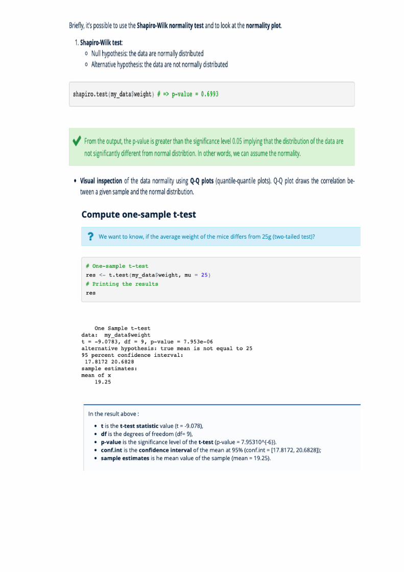
Note that, one-sample t-test can be used only, when the data are normally distributed (data should be of bell-shape, the mean and median are equal, and 68% of the data fall within 1 standard deviation). This can be checked using Shapiro-Wilk test.

http://www.sthda.com/english/wiki/one-sample-t-test-in-r

9.8 Testing the Mean of a Sample (t Test) (read

from R-cookbook)

Problem: You have a sample from a population. Given this sample, you want to know if the mean of the population could reasonably be a particular value m.

Solution

Apply the t.test function to the sample x with the argument mu=m:

> t.test(x, mu=m)

The output includes a p-value. Conventionally, if p < 0.05 then the population mean is unlikely to be m whereas p > 0.05 provides no such evidence. If your sample size n is small, then the underlying population must be normally distributed in order to derive meaningful results from the t test. A good rule of thumb is that “small” means n < 30.

t.test(x, ...) ## Default S3 method: t.test(x, y = NULL, alternative = c("two.sided", "less", "greater"), mu = 0, paired = FALSE, var.equal = FALSE, conf.level = 0.95, ...)

ArgumentsX a (non-empty) numeric vector of data values.

Y an optional (non-empty) numeric vector of data values.

alternative a character string specifying the alternative hypothesis, must be one of "two.sided"(default), "greater" or "less". You can specify just the initial letter.

Mu a number indicating the true value of the mean (or difference in means if you are performing a two sample test).

paired a logical indicating whether you want a paired t-test.

Calculating the Statistic / Test TypesThere are three main types of t-test: An Independent Samples t-test compares the means   for two

groups. A  Paired sample t-test  compares means from the same group at

different times (say, one year apart). A one-sample t-test tests the mean of a single group against a

known mean.

--------------------------------------------------------------------------------

9.9 Forming a Confidence Interval for a Mean (read from R

cookbook)

--------------------------------------------------------------------------------

9.10 Forming a Confidence Interval for a Median

> wilcox.test(x, conf.int=TRUE) Wilcoxon signed rank test

data: x

V = 465, p-value = 1.863e-09

alternative hypothesis: true location is not equal to 0

95 percent confidence interval:

0.4235421 0.8922106

sample estimates: (pseudo)median 0.6249297

You can change the confidence level by setting conf.level, such as conf.level=0.99 or other such values. The output also includes something called the pseudomedian, which is defined on the help page. Don’t assume it equals the median; they are different: > median(x) [1] 0.547129

Discussion Suppose you encounter some loudmouthed fan of the Chicago Cubs early in the base- ball season. The Cubs have played 20 games and won 11 of them, or 55% of their games. Based on that evidence, the fan is “very confident” that the Cubs will win more than half of their games this year. Should he be that confident? The prop.test function can evaluate the fan’s logic. Here, the number of observations is n = 20, the number of successes is x = 11, and p is the true probability of winning a game. We want to know whether it is reasonable to conclude, based on the data, that p > 0.5. Normally, prop.test would check for p not equal to 0.05 but we can check for p > 0.5 instead by setting alternative="greater":

Questions Related to this Topic

2. for question 11, calculate Z-Score

15. ## Hamilton depression scale factor measurements in 9 patients with ## mixed anxiety and depression, taken at the first (x) and second ## (y) visit after initiation of a therapy (administration of a ## tranquilizer). x <- c(1.83, 0.50, 1.62, 2.48, 1.68, 1.88, 1.55, 3.06, 1.30) y <- c(0.878, 0.647, 0.598, 2.05, 1.06, 1.29, 1.06, 3.14, 1.29)Use Wilcox.test and analyze the result.

Notes

To study more on t-test---https://www.analyticsvidhya.com/blog/2019/05/statistics-t-test-introduction-r-implementation/

What is Dispersion in Statistics?

Dispersion is the state of getting dispersed or spread. Statistical dispersion means the extent to which a numerical data is likely to vary about an average value. In other words, dispersion helps to understand the distribution of the data.

Measures of Dispersion

In statistics, the measures of dispersion help to interpret the variability of data i.e. to know how much homogenous or heterogenous the data is. In simple terms, it shows how squeezed or scattered the variable is.

Types of Measures of Dispersion

There are two main types of dispersion methods in statistics which are:

Absolute Measure of Dispersion Relative Measure of Dispersion

Absolute Measure of DispersionAn absolute measure of dispersion contains the same unit as the original data set. Absolute dispersion method expresses the variations in terms of the average of deviations of observations like standard or means deviations. It includes range, standard deviation, quartile deviation, etc.

The types of absolute measures of dispersion are:

1. Range: It is simply the difference between the maximum value and the minimum value given in a data set. Example: 1, 3,5, 6, 7 => Range = 7 -1= 6

2. Variance: Deduct the mean from each data in the set then squaring each of them and adding each square and finally dividing them by the total no of values in the data set is the variance. Variance (σ2)=∑(X−μ)2/N

3. Standard Deviation: The square root of the variance is known as the standard deviation i.e. S.D. = √σ.

4. Quartiles and Quartile Deviation: The quartiles are values that divide a list of numbers into quarters. The quartile deviation is half of the distance between the third and the first quartile.

5. Mean and Mean Deviation: The average of numbers is known as the mean and the arithmetic mean of the absolute deviations of the observations from a measure of central tendency is known as the mean deviation.

Example: Sample From a PopulationSample 2 items from x

>x

[1] 1 3 5 7 9 11 13 15 17 > # sample 2 items from

x

> sample(x, 2)

[1] 13 9

example to simulate a coin toss for 10 times.

> sample(c("H","T"),10, replace = TRUE)

[1] "H" "H" "H" "T" "H" "T" "H" "H" "H" "T"

https://www.dezyre.com/article/100-data-science-in-r-interview-questions-and-answers-for-2018/187