€¦ · web viewsince the return to democracy in 1990, chile has pursued a development strategy...

LACEA 2104 Submission

How well has Social Protection Scheme Reduced Household Vulnerability in Chile?

Javier Bronfman1 and Maria S. Floro

Abstract: This paper empirically investigates the impact of Chile’s social protection’s monetary subsidies on vulnerability to poverty during 1996-2006. Using the National Socioeconomic Characterization household panel survey data, we adopt the Chaudhuri et al. (2002) method to estimate vulnerability. Since access to monetary transfers is not random, we use the propensity score matching method to address the problem of selection bias in testing the effect of these transfers. The effect of social protection subsidies on vulnerability is also examined on two groups namely, the transitory poor and the chronic poor. Our results suggest that the impact of the monetary transfers is mixed. They tend to help lower the vulnerability of individuals in chronic poor households who received continuous monetary transfers, but not those in transient poor households. The results suggest possible miss-targeting of the monetary subsidies and the presence of “vulnerability traps” for which these monetary transfers are inadequate.

Keywords: Vulnerability; social protection; monetary subsidies; poverty reduction; Chile. JEL Codes: I32; I38.

1 PhD student School of Public Affairs, American University and Associate Professor, Department of Economics, American University respectively. Email correspondence: [email protected] , The authors would like to thank the paper discussants at the 2012 Eastern Economics Association Meetings, 2012 and Paul Winters for their helpful comments and suggestions.

1

mailto:[email protected]


I. Introduction

One of the main accomplishments of Chile during the past two decades has been the significant reduction in poverty, from 39% in 1990 to 14% in 2006.2 Since the return to democracy in 1990, Chile has pursued a development strategy that has emphasized growth with equity, based on the notion that both are necessary in order to attain sustainable economic progress and human development. A number of studies highlighted two major reasons for this substantial poverty reduction (Larrañaga, 1994; Contreras, 1996; Contreras, 2001; Pizzolito, 2005). One was the significant growth in employment and wage earnings that accompanied the overall economic growth (at least until the economic crisis of the late 1990s).3 A second major reason was the government provisioning of social protection since 1990 through the expansion of social services and the provision of monetary transfers to vulnerable groups and to combat poverty.4 These social programs did not represent a dramatic shift away from the market liberalization and privatization policies adopted in the early eighties but rather, allowed an expanded set of social programs called Red de Protección Social (PROTEGE) to be established alongside these economic policies.

The government of Patricio Aylwin first undertook a number of poverty reduction and social protection programs under the Red de Protección Social scheme in order to uplift the poor by providing monetary subsidies to the elderly, indigenous groups, the disabled and women micro-entrepreneurs. Throughout the 1990s and early 2000, the government of Chile continued to improve the quality of the programs and employed better targeting mechanisms.5 In recent years however, there is growing concern on the extent of vulnerability among low-income households in Chile, particularly on their ability to cope with the multiple risks they face amidst a climate of heightened uncertainty. Much of this concern is related to the adverse effects of market liberalization policies leading to the persistence of high inequality and growing employment insecurity. In spite of the reduction of poverty in the last 20 years, evidence shows that vulnerability to poverty remains a problem. In fact, it is estimated that about 30 percent of the population in mid-2000 have incomes within 40 percent above of the official poverty line (Lopez and Miller 2008). Significant segments of the population could fall into poverty if hit by adverse shocks (Solimano, 2008, p. 26).

In recent years, several studies have indicated that standard measures of poverty, based on defined income-based or consumption-based poverty lines, do not convey

2 MIDEPLAN (2010)3 Investment rate in the 1990s reached up to more that 25 percent of the GDP and domestic savings rate was substantially high as well.4 The strong export growth experienced by Chile along with good fiscal management enabled the country to turn its budget deficit during the 1980s into a surplus. Accompanied with tax reforms, new concessions and private-public partnerships (particularly in large infrastructure projects) provided additional financial resources for the social protection scheme.5 Arellano, (2004)

2


adequate information on the vulnerable state that many households face, particularly in the face of income or consumption shocks. Households, even those that are above the poverty line, can fall into poverty due to a decline in their earnings and/or job security or, simply, to their inability to smooth their incomes amidst persistent variability in earnings. Households may also experience consumption shocks e.g., serious health/illness, increase in food prices or schooling expenditures, etc., which can shift their relative asset or resource position and thereby move them to poverty. A focus on the likelihood of being poor, rather than on observed levels of poverty at a given time, can provide a better understanding of poverty as a process and the longer-term consequences in well-being.

While a number of studies have examined the impact of Chile’s social protection scheme on poverty, none have analyzed its impact on household vulnerability.6 This paper attempts to fill in this gap by empirically investigating the vulnerability effect of Chile’s poverty social protection programs during 1996-2006 period. It makes use of 10,287 individuals respondents who were surveyed in the 1996, 2001 and 2006 waves of the CASEN (Encuesta de Caracterización Socioeconómica Nacional) panel household survey. We define vulnerability to poverty in our paper as a forward-looking measure of the level of exposure to future risks, shocks and proneness to economic insecurity that can undermine the household’s survival and the development of its members’ capabilities. For the non-poor, it refers to the risk of falling into poverty; and among the poor, staying poor or becoming even poorer (Kamanou and Morduch, 2005). For our study, we adopt the Chaudhuri, Jalan and Suryahadi, (2002) method for estimating vulnerability and use Average Treatment Effect on the Treated (ATT) approach with propensity score matching adjustments for evaluating the effect of Chile’s monetary transfer-based social protection schemes on vulnerability.7 We also examine the effect of these schemes on two groups, the transitory poor and the chronic poor.

This paper is organized as follows. Section 2 describes Chile’s social policy during the period 1990-2006. A review of the relevant literature on poverty dynamics and vulnerability is given in Section 3. The next section (Section 4) explains the data and methodology used in our empirical analysis and presents the results. A summary of the main study findings and their implications for policy and future research concludes the paper.

II. Chile’s social protection program after 1990One of the defining features of the Chilean government policies, after the country’s return to democracy in 1990, was the expansion of social protection and poverty alleviation programs as part of the “growth with equity” development strategy.8 Chile’s market

6 See: Arellano (2004); Agostini, Brown and Góngora (2010); Agostini and Brown (2011); Contreras (2003) among others.7 Also in Chaudhuri (2003).8 Chile’s social protection scheme encompasses the work of various ministries which implement programs and benefits such as scholarships, monetary transfers, health services, disability and unemployment insurance, etc. (Waissbluth,

3


liberalization policies in the eighties enhanced economic growth but have also increased poverty for large segments of the population. Although Chile experienced per capita growth as shown in Figure 1, averaging 5.5 % annually since the mid-eighties, it had a high poverty rate of 38% in 1990.

Figure 1. Chile’s per capita gross domestic product growth rate 1985-2009 and social expenditure as a percentage of GDP 1985-2009

-5.0

0.0

5.0

10.0

15.0

20.0Yearly per capita GDP growth rate

Social expendi-ture as a per-centage of GDP

Perc

enta

ge r

ate

Source: Statistical yearbook for Latin America and the Caribbean, ECLAC (2010), and Estadísticas de las Finanzas Públicas. DIPRES, Chilean Ministry of Finance. Note: Annual percentage growth rate of GDP at market prices based on constant local currency.

For the newly elected Aylwin government and its successors, improved access to social safety nets such as social security, unemployment and disability insurance as well as basic health and social services were deemed critical to prevent those with the least resources from falling (deeper) into poverty and to help generate better opportunities for the poor. Government social expenditures as a percentage of the total government expenditures rose from 61% in 1990 to 67% in 2006 (see Appendix A). Much of the increase in public spending was financed by the 1990 tax reforms and increased government revenues resulting from high levels of export and economic growth. The tax reform helped increased Chile’s tax revenue from 14% of GDP in 1990 to 16.4% of GDP in 2002, thus providing the needed funds to advance its social policy without incurring large fiscal deficits (Arellano 2004). Moreover, the government not only increased the level of social spending but also implemented reforms aimed at improving the effectiveness and quality of the existing social programs. The importance of social spending in poverty reduction is highlighted in Weyland (1999) and Solimano (2008)

2005, p.75)

4


who noted that each percentage point of economic growth contributed 50% more towards reducing poverty under the Concertación9 from 1990 to 1996.

To allocate monetary subsidies, the government of Chile has developed in the eighties, a social characterization record card called “Ficha CAS”. During the period 1990-2005, the “Ficha CAS” was used to identify the potential beneficiaries of social programs and government assistance by distinguishing poor and non-poor households and by sorting them according to their needs.10 This tool applied conventional measures of poverty and made use of several social and economic indicators that were then weighted, yielding a computed poverty score that ranges from 380 to 770 points.11 Households that scored below 501 points were considered severely poor, and those with 501-540 points were considered poor (see Appendix B). It allowed for the decentralization of resource allocation and government assistance, and was implemented at the municipal level, although the Ministry of Planning, Mideplan, remained in charge of providing the information for identifying the beneficiaries. The Red de Protección Social (PROTEGE) involves a number of programs that provided monetary subsidies (see Appendix C). Household eligibility for these subsidies during the 1996-2006 period was based on their score (in the Ficha CAS) that places them in the second quintile of “social vulnerability”. Their score is based on the evaluation of the local government using the “Ficha CAS” criteria. Hence, there is likely to be some self-selection with regards to access and participation in the PROTEGE social programs. This is an issue that we later address in the methodology section of the paper.III. Examining Poverty and Household Vulnerability in Chile

9 “Concertación”: Concertación de Partidos por la Democracia represents a center-left political parties coalition founded in 1988, with the purpose to with the presidential elections and end the military government. 10 The original “Ficha CAS”, developed in 1980, was based on the following components: housing characteristics (number of rooms, construction materials, access to water and sanitation, access to electricity and overcrowding), education (household head’s years of schooling), occupation (referring to the highest occupational category between spouses or that of household head), household income, and value of assets. This allocation instrument was revised in 1987 and referred to as “Ficha CAS-II”. It made use of fifty characteristics, which were assessed using principal component and discriminant factor analysis. In 1999, the CAS-II was updated by excluding some variables that were considered ineffective predictors of poverty. See Clerk and Wodon (2001) and Larrañaga (2005) for a detailed discussion of “Ficha CAS”. 11 In 2006, the “Ficha CAS II” adopted a new framework, one that is based on the notion of entitlements. The eligibility criteria for accessing social protection programs and government assistance has shifted from being mainly based on income poverty status to a more comprehensive list of vulnerability indicators and adopted a new name “Ficha de Protección Social” (FPS). The FPS identifies vulnerability according to three sources namely: a) access to economic resources, b) household needs, and c) risks faced by households. Economic resources include income generation capacity or work skills of individuals, access to potable water and sewer system, home ownership, and relationship between family size and house size. Needs are based on household size, family composition and related characteristics. Risks include individual-based risks such as health condition, disability and job insecurity, as well as geographical location-based risks such urban-rural area and local unemployment rate. The new instrument, called the Social Protection Record Card or “Ficha de protección social (FPS)”, acknowledges the multiple dimensions of poverty. It should be noted however that poverty reduction and social protection programs do not solely base their eligibility on the calculated score; some also specify other requirements that prevails over the estimated FPS score such as disability, old age, childbearing etc.

5


Several studies have attributed Chile’s success in poverty reduction to a variety of factors. Arellano (2004) study highlights the role of fiscal prudence and management in enabling the government to increase social spending and reduce poverty. This involved a reduction of the government infrastructure spending by focusing on those projects which have large social benefits and which the private sector was underproviding. The government also reduced the defense budget from 2.3% of GDP in 1990 to 1.2% by 2006.12 Such efforts to maintain fiscal responsibility have helped reduce the national debt to a quarter of its 1990 level, further freeing up additional resources. It also promoted public-private sector partnerships in several of its social programs, thereby increasing the financing of (government-guaranteed) education loans, microenterprise development, and housing loans among others. The above initiatives helped expand the coverage and improve the effectiveness of the social programs, thereby reducing income poverty to 23.2% in 1996 and further to 13.7% by 2006 (Figure 2).

Figure 2.Poverty and extreme poverty rate 1990-2006

1990 1992 1994 1996 1998 2000 2003 200605

1015202530354045

38.632.9

27.623.2 21.7 20.2 18.7

13.7139 7.6 5.7 5.6 5.6 4.7 3.2

Total PovertyExtreme poverty

Source: Authors’ calculations using CASEN data for each year. Poverty and severe poverty rates are based on the national (income) poverty line and the national (income) extreme poverty line respectively. See Mideplan (2009) for estimation.

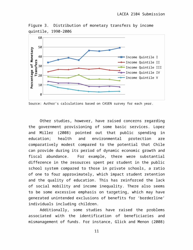
Larrañaga (1994) and Contreras (2003) argued that poverty reduction in Chile has been due to the pro-poor growth strategies implemented since 1990. Using the Datt-Ravallion decomposition, they estimated that economic growth accounted for over an 80% of the reduction in poverty in the period 1990-1996. By examining quintile-level income changes over time, Contreras, Cooper, Hermann and Neilson (2005) argued that Chile’s growth benefited poor people in the sense that they experienced a larger share of the income growth, compared to individuals in higher quintiles. This positive effect is also due to the social protection programs that provided safety nets in the form of cash transfers and subsidies especially to the lowest quintile. Table 1 and Figure 3 show the percent distribution of monetary transfers and subsidies from 1990 to 2006 by income quintile. The proportion received by those in the lowest quintile increased from 34% in 1990 to 36.2% in 1996 to nearly 50% by 2006. Over the same period, the proportion of

12 Estado de operaciones del Gobierno Central www.dipres.gov.cl/572/articles-45410_doc_pdf_Funcional 3.pdf

6


total monetary subsidies received by the richest (quintile declined from 10.2% in 1990 to 3.2% in 2006.

Table 1. Percentage of total monetary subsidies received by income quintile 1990-2006Income Quintile

Year I II III IV V1990 33.7 23.8 18.5 13.8 10.21992 36.6 26.3 17.7 12.0 7.41994 38.7 26.2 17.3 12.1 5.71996 36.2 27.7 20.5 11.5 4.11998 46.3 26.5 15.9 8.5 2.92000 45.7 27.4 16.0 8.3 2.62003 46.8 25.7 15.7 8.7 3.12006 49.3 25.2 14.3 8.0 3.2

Source: Authors’ calculations from using CASEN data (Mideplan, 2009).

Figure 3. Distribution of monetary transfers by income quintile, 1990-2006

1990 1992 1994 1996 1998 2000 2003 20060

10

20

30

40

50

60

Income Quintile IIncome Quintile IIIncome Quintile IIIIncome Quintile IVIncome Quintile V

Perc

enta

ge o

f Mon

etar

y T

rans

fers

Source: Author’s calculations based on CASEN survey for each year.

Other studies, however, have raised concerns regarding the government provisioning of some basic services. Lopez and Miller (2008) pointed out that public spending in education; health and environmental protection are comparatively modest compared to the potential that Chile can provide during its period of dynamic economic growth and fiscal abundance. For example, there were substantial difference in the resources spent per student in the public school system compared to those in private schools, a ratio of one to four approximately, which impact student retention and the quality of education. This has reinforced the lack of social mobility and income

7


inequality. There also seems to be some excessive emphasis on targeting, which may have generated unintended exclusions of benefits for ‘borderline’ individuals including children.

Additionally, some studies have raised the problems associated with the identification of beneficiaries and mismanagement of funds. For instance, Glick and Menon (2008) mentioned that some households might purposely underreport incomes and assets in order to avail of the subsidies. Evidence is provided by Agostini and Brown (2007) who found that a proportionately larger share of monetary transfers (using 2003 data) went to households in the top half of the income distribution. Misrepresentation seems to have occurred at higher levels of aggregation as well.13 Hence, the social protection and poverty alleviation programs may not be well targeted and could have been subjected to mismanagement. In addition these social programs did not necessarily represent a dramatic shift away from the market liberalization policies adopted in the early eighties, rather they were establish alongside these economic policies. As a result, social reforms have not been able to address the high levels of inequality, particularly evident in health and educational outcomes (World Bank, 1997).

IV. Literature reviewPoverty is a paramount concern when monitoring development progress. However, standard poverty indicators are ex-post measures which overlook the multiple risks that individuals or household may face and their ability/resources (or lack thereof) to cope and avoid becoming poor (or poorer) in the future. There are, by now, some evidence, which indicate that a large proportion of the population in developing countries is vulnerable to poverty. The Chronic Poverty Report (2005), for example, indicates that although the estimated population share who are chronic poor in Latin America ranges from 30 to 40 percent, those considered to be transitory poor (i.e., individuals that at least once during the period of study fell below a poverty threshold) appears to be relatively much larger. Income variability that arises from fluctuations in earnings particularly in temporary or informal employment, can affect households’ ability to manage risk and cope with shocks. Poor quality of public services e.g., healthcare can aggravate household exposure to health shocks. Thus, even though average household incomes do not fall into poverty levels, the degree of household vulnerability can be high, leading to increased debt or sale or pawning of assets.

Given the inadequacy of poverty measures to deal with the future economic situation of households, a growing number of studies have focused on measuring vulnerability to poverty. To date, there exist a number of vulnerability measures but for the most part, they require longitudinal datasets to explore the dynamics of poverty, which are scarce in developing countries (Günther and Harttgen 2009).

13 For example, although municipalities know best what their needs are, decisions regarding development spending are taken at the nation-wide level. As a consequence, “…municipalities have an incentive to exaggerate their list of planned projects…” , presumably in order to influence government spending. (Cited in Glick and Menon 2008).

8


Chaudhuri et al. (2002) proposes a method of estimating vulnerability that allows the use of limited longitudinal household data. Their approach overcomes the data availability issue by utilizing two or more time period cross-sectional data and focusing on the error term. It assumes that a household’s vulnerability level derives from the stochastic properties of the (unobserved) inter-temporal consumption stream that it faces, and these in turn, depend on pertinent individual and household characteristics and the characteristics of the environment it operates.

The Chaudhuri et al. approach has been utilized in a number of studies on vulnerability. Günther and Harttgen (2009) expanded the Chaudhuri et al. (2002) approach in their multi-level analysis of vulnerability for Madagascar. The study takes into account the effects on household consumption of idiosyncratic and covariate shocks in the rural and urban areas. Bourguignon and Goh (2004) estimated vulnerability by using repeated cross-sectional data to create a pseudo-panel data and then compared their results with actual panel data. They concluded that under certain assumptions, both estimates are very similar (particularly in trend and average estimates). Their findings indicate job loss as the most important factor affecting vulnerability.

Zhang and Wan (2008) also adopted the Chaudhuri et al. approach using panel data from China to estimate household vulnerability and test their reliability. Their findings indicate that vulnerability measures are more reliable when using the 2 USD (instead of the 1 USD) as poverty line, when the estimation of permanent income assumes a log-normal distribution, and when the vulnerability threshold is set at 50 per cent of probability of being poor in the future. The Chaudhuri et al. method has also been adopted by Imai, Wang and Kang (2009) in their analysis of the impact of taxation on poverty and vulnerability in rural China. Likewise, Jha, Imai and Gaiha (2009) assessed the impact of two public works and food subsidies programs in India on (consumption) poverty and vulnerability. Using a treatment effect model with propensity score matching approach, the authors found a significant and negative effect of participation on poverty, malnutrition and vulnerability.

A number of studies have examined poverty dynamics and income mobility in Chile. One of the early works is by Scott (2000), who used a small rural household panel data from 1968-1986. His findings suggest very small income mobility among the rural population; any poverty reduction during the period was mainly due to social policy transfers and subsidies. Aguilar (2002), using the first wave of the Panel CASEN survey for 1996-2001 also analyzed income mobility in Chile and found that household size and lack of or low quality of employment to be main determinants of poverty. He also found that poor households do not make extensive use of government safety nets when faced with negative shocks; instead, they resort to assistance by kin. Using the same dataset as Aguilar (2002), Castro and Kast (2004) found evidence of income mobility, with 32% of people in Chile having lived below the poverty line at some point during the five year- survey period. Their study also showed correlation between poverty and labor market employment, particularly the nature of informal employment. This finding is confirmed

9


by Neilson, Contreras, Cooper and Hermann (2008).14 Chronic poverty in particular, is found to be directly related to unemployment and lack of human capital (as measured by level of education). The effect of household size and composition as well as female headship on poverty and income mobility is pronounced in Zubizarreta (2005).

The issue of vulnerability has been directly examined by Rodriguez, Dominguez, Undurraga and Zubizarreta (2008) and Bronfman (2010), using CASEN panel data for 1996-2001 and 1996-2006 periods respectively. Rodriguez et al. (2008) constructed an adjusted poverty index using vulnerability and explored its determinants. Their results indicate that lack of human capital and certain household characteristics such as household size and proportion of elderly members significantly determine vulnerability. However, this article only looks at the working population in the Metropolitan region. The Bronfman (2010) study confirmed the findings reached by Neilson et al. (2008) and Castro and Arzola (2008) regarding movements of a large segment of the population in and out of poverty. More recently, Cruces et al. (2010), in a cross-country study of Latin America, point to a much higher rate of vulnerability compared to poverty estimates, although he argued that aggregate vulnerability in the region has decreased over the period early 1990s-mid 2000.15 None of these studies however have examined directly the effect of social protection on vulnerability. A few studies that examined the impact of government cash transfers or monetary subsidies in Chile focused on poverty. For example, Agostini and Brown (2007a, 2007b) found that monetary subsidies had a positive effect on reducing poverty and inequality at the aggregate level. A later study by Agostini, Brown and Góngora (2008) emphasized the role of local government finance and strength of government mandates in mediating the effectiveness of monetary subsidies. More specifically, they found evidence regarding the significant impact of public expenditures on the efficiency of monetary transfers and a weak influence by the strength of the mayor´s mandate.

Our paper builds on the previous work on vulnerability and poverty dynamics in Chile and other developing countries by updating previous vulnerability estimations and more substantively by examining the effect of social protection on vulnerability to poverty, using Chile’s social protection scheme of allocating monetary subsidies during 1996-2006 period as case study. In particular, we assess how access to monetary transfers affects household vulnerability using a the ATT estimation approach. Unlike previous impact studies on these programs, we make use of propensity score matching in order to correct for selection and endogeneity bias in our estimations.V. Empirical Analysis and Results

a. Data and Methodology

14 Differentiating between chronic and transitory poor, Neilson et al (2008) estimated that 20,2% and 18.3% of the population were poor in 1996 and 2001 respectively. However, more than 30% of the people lived under the poverty line for at least in one of the periods, and 9% were chronically poor (poor in both years).15 The study made use of the $2 and $4 per person per day international poverty lines in their poverty estimates.

10


Our analysis makes use of the 10,287 survey-respondents in the 1996, 2001 and 2006 waves of the National Socio Economic Characterization Survey (“Encuesta de Caracterización Socioeconómica Nacional”, better known as CASEN).16 Although the CASEN surveys typically do not have the same household sample for each year, a special subsample based on the 1996 National Socio Economic Characterization Survey respondents from 4 regions were randomly re-surveyed in 2001(second wave) and 2006 (third wave).17 Figure 4 shows the attrition rate associated with the panel survey data, with the number of retained or original (1996) survey respondents in the subsequent (2001, 2006) samples represented by the dark areas. The decline in the number of retained respondents shows the extent of the attrition problem over time. The light gray section of the bar represents the newly added respondents. Since the survey is based on households as well as individuals, new members of original families became part of the latter samples. The attrition rate for the 1996-2001 period is 28.1%, and 50.9% for the 1996-2006 period.18 To address this issue, population weights, which were constructed by the Ministry of Planning and the University Alberto Hurtado “Fundación para la Superación de la Pobreza”, are used in the 2001 and 2006 surveys in order to correct for any attrition bias and to maintain representativeness of the survey sample.19

Figure 4. Number of interviewed individuals in different waves of the CASEN data

Source: Bendezú et al. (2007). The “new respondents” came from the original families interviewed in 1996 who have established their own households.

We adopt Chaudhuri’s et al. (2002) estimation method and use the average treatment effect (ATT) on the treated estimation with propensity score matching (PSM)

16 National and regional representative surveys have been conducted every two or three years (1985, 1987, 1990, 1992, 1994, 1996, 1998, 2000, 2003, 2006 and 2009) and are deemed reliable.17 Chile has 13 regions at the time of the survey; the 4 regions namely: III, VII, VIII and the Metropolitan Region. were covered in the CASEN, representing 60% of total population.18 This attrition rate is considered reasonable for a 10-year, three-wave panel data.19 For a complete discussion on the panel CASEN attrition problem and data quality, see Bendezú et al. (2007) and PNUD (2009).

11

Vulht Pr Yh,t1PL


approach to evaluate the effect of monetary transfers on vulnerability. Our estimation of vulnerability is based on the assumption of a unitary household and is expressed as:20

where vulnerability of household h in time t is equal to the probability of future income Yh, t+1 being below a threshold i.e. income-based poverty line, PL.21 The future income is estimated as a function of observable characteristics, Xh and an error term eh that captures the idiosyncratic shocks as shown in:

(2)

Substituting (2) into (1) equation yields the following vulnerability equation:

(3)

We then estimate the log income equation:

(4)

where Yh,t is the household income per capita in time t, and Xh,t represents the set of pertinent individual (head) and household characteristics. These include: sex, life cycle stage (age, age square) years of education, wealth proxy (home ownership dummy), labor force status-based proxy variables for earnings insecurity (unemployed dummy, domestic service worker dummy, self-employed dummy), household structure, household size, presence of children (under 7 years old), and employed members to household size ratio. We also include regional dummy variables to control for region-level fixed effects.

Keeping the predicted output = and the residual , we next estimate the

expected log income, and variance for each household, using a three step

feasible generalized least square (Amemiya, 1977) yielding:

20 Given data limitations, we make use of the unitary household model that assumes income and resources are pooled and are shared equally among members of the household. 21 Both household income and income poverty line are expressed in per capita terms.

12

Vulh Pr LnYh LnPL LnPL Xh

Xh


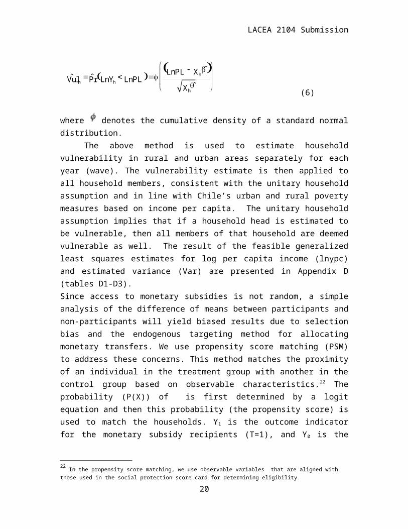
(5a,b) Assuming a log normal distribution for income, we estimate vulnerability using the reduced form:

(6)

where denotes the cumulative density of a standard normal distribution. The above method is used to estimate household vulnerability in rural and urban areas separately for each year (wave). The vulnerability estimate is then applied to all household members, consistent with the unitary household assumption and in line with Chile’s urban and rural poverty measures based on income per capita. The unitary household assumption implies that if a household head is estimated to be vulnerable, then all members of that household are deemed vulnerable as well. The result of the feasible generalized least squares estimates for log per capita income (lnypc) and estimated variance (Var) are presented in Appendix D (tables D1-D3). Since access to monetary subsidies is not random, a simple analysis of the difference of means between participants and non-participants will yield biased results due to selection bias and the endogenous targeting method for allocating monetary transfers. We use propensity score matching (PSM) to address these concerns. This method matches the proximity of an individual in the treatment group with another in the control group based on observable characteristics.22 The probability (P(X)) of is first determined by a logit equation and then this probability (the propensity score) is used to match the households. Y1 is the outcome indicator for the monetary subsidy recipients (T=1), and Y0 is the outcome indicator for the non-recipients (T=0), then equation (7) denotes the mean impact:

(7)

where the propensity score matching estimator is the mean difference in the outcomes over common support, weighted by the propensity score distribution of recipients. Since the probability of two households being exactly matched is close to zero, distance measures are used to match households so we use the nearest neighbor (NN) algorithm.23 This algorithm is the most straightforward and matches partners according to their 22 In the propensity score matching, we use observable variables that are aligned with those used in the social protection score card for determining eligibility.

13

)(,0|)(,1| 01 XPTYEXPTYE


propensity score. We also estimate the Kernel method, which uses the weighted average of nearly all individuals in the control group to construct the counterfactual outcome. Bootstrapped standard errors for the above procedures are used as well.

It should be noted that the vulnerability thresholds in these models are admittedly arbitrary. We therefore follow Chaudhuri’s proposed thresholds and compare our estimations using two different “vulnerability thresholds”. First, a household is considered vulnerable if the calculated probability of their predicted log per capita income is below the national poverty rate. Second, we consider a high vulnerability threshold of at least 50% probability of becoming poor in the future.

b. ResultsPoverty, vulnerability and high-vulnerability estimates for rural and urban respondents in 1996, 2001 and 2006 are presented in Table 2. Both household and per capita (individual) vulnerability estimates are reported, with the latter typically being slightly higher than household-level estimates.24 Throughout the period 1996-2006, the estimated vulnerability rates are shown to be much higher than the observed poverty rates, particularly in the urban areas. Although poverty rates continued to decline, we observe an initial decline in individual vulnerability from 49.3% in 1996 to 42.5% in 2001, but this rises to 49.2% in 2006. (Similar trends are found for household-level vulnerability). This trend is also true in terms of high vulnerability (50% or above probability of becoming poor), at least for the urban respondents. In the rural areas, per capita or individual high vulnerability estimates appear to decline significantly between 1996 and 2001, then continues to do so more slowly in 2001-2006. This trend however is not observed for rural household high vulnerability rates, which suggests that the observed decline in per capita high vulnerability between 2001 and 2006 may be due to a reduction in household size. Overall, the estimates in Table 2 show that even though poverty has fallen significantly throughout the reference period, vulnerability to poverty has not showed the same trend over time. In particular, urban households and individuals experienced a significant increase in their vulnerability from 2001 to 2006, showing a convergence with the rural areas.

23 For further discussion on difference in difference PSM, see Becker and Ichino (2002), Caliendo and Kopeining (2005), Abadie et al. (2004), Abadie and Imbens (2002), Imbens (2004), Heckman, Ichimura, and Todd (1998), and Wooldridge (2002) among others. 24 This may be explained by the fact that poorer households tend to be larger in size.

14


Table 2. Poverty, vulnerability and high vulnerability rates for 1996, 2001, 2006, urban and rural households and individuals.

1996 2001 2006Urban Rural Total Urban Rural Total Urban Rural Total

Household Poverty rate 18.6% 28.6% 19.8% 15.3% 20.7% 15.9% 9.2% 12.1% 9.6%Individual Poverty rate 22.9% 33.6% 23.6% 19.6% 25.1% 20.2% 10.2% 13.0% 10.5%Household Vulnerability 41.8% 43.2% 41.9% 34.4% 34.9% 34.6% 47.6% 45.9% 47.4%Individual Vulnerability 48.9% 51.3% 49.3% 42.7% 41.1% 42.5% 49.1% 49.5% 49.2%Household High-Vulnerability (50%)

13.6% 24.2% 14.8% 12.0% 14.7% 12.4% 16.7% 17.0% 16.7%

Individual High-Vulnerability (50%)

17.3% 30.3% 18.8% 16.4% 18.2% 16.6% 17.2% 16.9% 17.2%

Source: Authors’ calculations using the CASEN 1996-2001-2006 panel data.

We next examine the predictive power of the vulnerability estimates by cross-tabulating vulnerability and high-vulnerability in 1996 and 2001 with the actual poverty rates in 2001 and 2006 respectively. We present the results for individual (per capita) in Tables 3 and 4; similar tables for household estimates are provided in Appendix F.25 About 34% of those individuals deemed vulnerable in 1996 fell into poverty in 2001, however only 10% of those considered vulnerable in 2001 became poor in 2006. The difference in the predictive power of individual vulnerability estimates between the two periods may be due to unexpected shocks faced by households in 1998-99 resulting from the economic crisis and/or to improvements in social protection targeting after 1999, enabling the monetary transfers to better assist those who are deemed vulnerable. Our high-vulnerability estimate yield higher poverty predictive power with 46.7% and 25% of those deemed as highly vulnerable.26

Table 3. Comparison of 1996 estimated individual vulnerability rate and 2001 poverty rate.

Poor in 2001No Yes

Vulnerability 1996No 93.0% 7.0%Yes 66.2% 33.8%

25 The household vulnerability estimates predict correctly the future poverty status for 28.2% and 17.1% of respondents in 1996 and 2001 respectively. About 6% of the predicted non-vulnerable households in 1996 and 4% in 2001 became poor in 2001 and in 2006 correspondingly.26 The tables providing the comparisons of vulnerability, high vulnerability and poverty rates for total population sample as well as for transitory poor and chronic poor groups are given in Appendix F.

15


High-Vulnerability 1996No 86.0% 14.0%Yes 53.3% 46.7%


Table 4. Comparison of 2001 estimated individual vulnerability rate and 2006 poverty rate

Poor in 2006No Yes

Vulnerability 2001No 95.3% 4.7%Yes 89.7% 10.3%High-Vulnerability 2001No 92.6% 7.4%Yes 75.0% 25.0%


A simple comparison of the percentage changes in vulnerability on the basis of access to and frequency of participation in the social programs is likely to suffer from selection bias, since local authorities select the social protection program recipients based on their household score of the proxy means-test targeting allocation tool. Therefore any mean differences could be a result of program participants’ selection process. We therefore need examine the impact of social protection monetary transfers on vulnerability analysis using multiple algorithms that take the selection bias from participation into account. Heckman et al. (1997) suggest that in small samples, the choice of the matching algorithm can be important due to trade-offs between bias and variances.

We first infer the counter-factual regarding what would have been the value of the outcome indicator in the absence of monetary subsidies, hence the role of non-recipients (control group) for each year (wave). Appropriate comparisons with control groups can then be made to assess the impact of the monetary subsidies on the recipients (treatment group). We use the propensity score matching (PSM) method to statistically create the treatment and comparison groups. To obtain a comparable group, the propensity score is estimated using proxy variables that are similar to those used in program targeting. The PSM uses the “Propensity Score” or the conditional probability of participation to identify a counterfactual group of non-recipients, given conditional independence. We adopt the observable characteristics used by the government in allocating monetary transfers in the PSM to address the problem of selection bias in our impact evaluation. Next, we apply the Average Treatment Effect on the Treated (ATT) method to compare the treatment and control groups for 1996 and 2001 waves in terms of changes in vulnerability estimates over time relative to the outcome observed in pre-

16


intervention baseline.27 This allows for conditional dependence on the levels arising from additive time-invariant latent heterogeneity.28 We use two different algorithms for propensity score matching to identify the comparison group. First, we use the Nearest Neighbor matching algorithm (NN) that matches each treated observation to a control observation with the closest propensity score.

We first estimate the ATT on two “treatment group waves” with respect to their vulnerabilities in the next period. The ATT is estimated using nearest neighbor as well as the kernel methods.

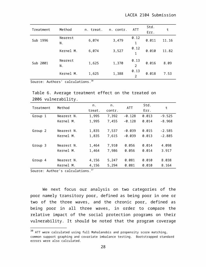
Table 5 presents the ATT impact estimations on 2001 vulnerability for individuals in households that received monetary transfers in 1996 (referred as 1996 treatment group) as well as on 2006 vulnerability for those individuals who received monetary transfers in 2001 (2001 treatment group). The results show a positive and statistically significant impact for both waves, which imply that having access to monetary transfers in 1996 seem to have increased vulnerability by 12% in 2001, both using nearest neighbor and kernel estimation methods. For those individuals in monetary transfer-recipient households in 2001, the effect on their vulnerability in 2006 is also positive and statistically significant, with a 13% increase in vulnerability. These may be due to the presence of a “vulnerability trap” in the sense that the monetary transfers were inadequate in assisting the individuals and their households to deal with sudden large shocks including serious illness, decline in earnings, increase in school expenditures, or job loss. We next categorize the individuals in the sample on the basis of household access to and frequency of participation in the program in order to explore the effects of monetary subsidies on vulnerability. Group 1 includes those individuals who did not received monetary subsidies in both 1996 and 2001. Since not all household beneficiaries received social protection cash transfers throughout the time period, we group them on the basis of frequency. Group 2 refers to those who received subsidies in 1996 but not in 2001. Group 3 refers to those who received subsidies in 2001 but not in 1996. Finally, Group 4 includes individuals who received subsidies in both 1996 and 2001.29

Table 6 presents the PSM-based average treatment effect on the treated (ATT) on individual vulnerability estimates for each group in 2006. The ATT estimates show the effectiveness of 1996 monetary transfers in decreasing vulnerability in 2006 for those in group 2, namely those individuals in households that received them in 1996 but not in 2001, experienced lower levels of vulnerability in 2006. However, individuals in groups 3 and 4, i.e. those who received monetary transfers in 2001 but not in 1996 as well as those receiving in both years appear to be worse off in terms of vulnerability, which indicate that the monetary subsidies received were not sufficient in lowering their 27 The PSM and ATT were calculated using full Mahalanobis, propensity score matching, common support graphing, and covariate imbalance testing methods. Bootstrapped standard errors were computed as well.28 The changes over time in the vulnerability estimator will likely contain some heterogeneity in the observables, which would bias an unmatched DID. Propensity score matching addresses possible observable heterogeneity between the two groups.29 Appendix E (tables E1-E6) shows the estimated individual vulnerability for each group category.

17


vulnerability. Not surprisingly, individuals in group 1 seem able to lower their vulnerability without any program assistance. Table 5. Average treatment effect on the treated (ATT) on vulnerability in next wave.Treatment Method n. treat. n. contr. ATT Std. Err. tSub 1996 Nearest N. 6,074 3,479 0.121 0.011 11.16

Kernel M. 6,074 3,527 0.121 0.010 11.82

Sub 2001 Nearest N. 1,625 1,370 0.132 0.016 8.09Kernel M. 1,625 1,388 0.132 0.018 7.53

Source: Authors’ calculations.30

Table 6. Average treatment effect on the treated on 2006 vulnerability.Treatment Method n. treat. n. contr. ATT Std. Err. tGroup 1 Nearest N. 1,995 7,392 -0.128 0.013 -9.525

Kernel M. 1,995 7,455 -0.128 0.014 -8.968

Group 2 Nearest N. 1,835 7,537 -0.039 0.015 -2.585Kernel M. 1,835 7,615 -0.039 0.013 -2.885

Group 3 Nearest N. 1,464 7,910 0.056 0.014 4.098Kernel M. 1,464 7,986 0.056 0.014 3.917


Source: Author’s calculations.37

We next focus our analysis on two categories of the poor namely transitory poor, defined as being poor in one or two of the three waves, and the chronic poor, defined as being poor in all three waves, in order to compare the relative impact of the social protection programs on their vulnerability. It should be noted that the program coverage was more extensive for the chronic poor, compared to the transitory poor and the entire population. We adopt the same four group categories in our application of the ATT approach. We perform two ATT tests for each of the poverty groups; the first is to assess the impact of the subsidies on vulnerability in the subsequent waves, and the second is to assess the overall impact of subsidies received in previous periods on individual vulnerability in 2006.

Table 7 shows the impact of monetary transfers in 1996 and 2001 on the vulnerability of the transitory poor in subsequent waves. The positive and significant signs show that access to monetary subsidies in 1996 increases the vulnerability in 2001; similarly access to monetary transfers in 2001 increased vulnerability in 2001. These

30 ATT were calculated using full Mahalanobis and propensity score matching, common support graphing and covariate imbalance testing. Bootstrapped standard errors were also calculated.

18


results could be driven individuals in group 4, who experienced an increased in vulnerability in 2006 as shown in Table 8.

The ATT results among transient poor households in Table 8 show that only individuals in group 1, i.e. those who didn’t receive any subsidies, showed a statistically significant decline in vulnerability. On the other hand, the transitory poor belonging to group 4 and who received subsidies both in 1996 and 2001 still experienced an increase in their vulnerability in 2006, a further indication of a vulnerability trap. However, we find a null effect for those households receiving subsidies in one of the waves (Groups 2 and 3). This indicates that after accounting for selection bias the vulnerability levels of transient poor who received monetary subsidies in 1996 only and in 2001 only, are not statistically significant different from those who did not.

Table 7. Average treatment effect on the treated on vulnerability in next wave: among the transient poor.

Treatment Method n. treat. n. contr. ATT Std. Err. tSub 1996 Nearest N. 3,079 1,417 0.066 0.013 4.995

Kernel M. 3,079 1,452 0.066 0.013 4.970

Sub 2001 Nearest N. 3,015 1,407 0.053 0.016 3.298Kernel M. 3,015 1,423 0.053 0.015 3.605


Table 8. Average treatment effect on the treated on vulnerability 2006: among the transient poor.Treatment Method n. treat. n. contr. ATT Std. Err. tGroup 1 Nearest N. 637 3,760 -0.073 0.019 -3.857

Kernel M. 637 3,801 -0.073 0.020 -3.661

Group 2 Nearest N. 786 3,607 -0.018 0.016 -1.128Kernel M. 786 3,652 -0.018 0.016 -1.117

Group 3 Nearest N. 772 3,620 0.007 0.020 0.337Kernel M. 772 3,666 0.007 0.018 0.372



For the chronic poor however, the ATT results presented in table 9 show no statistically significant effects on vulnerability 2001 and 2006 as a result of the social protection subsidies in 1996 and 2001 respectively. The group- specific effects of the monetary subsidies among the chronic poor may explain these results, as shown in Table 10. The nearest neighbor and kernel matching algorithms show statistically significant and negative effects on vulnerability among chronic poor individuals in households that

19


had access to subsidies in 1996 and 2001 (Group 4), which suggests that continuous provision of monetary transfers seem to have helped reduce the vulnerability of the chronic poor. However, those individuals who received subsidies in 1996 but were dropped in 2001 (group 2) experienced an increase in vulnerability by 2006. The null effect on group 3, as with group 1, indicate the insignificant impact of the social programs on their vulnerability, after accounting for selection bias, compared to those who did not. Table 9. Average treatment effect on the treated on vulnerability in next wave: among the chronic poor.

Treatment Method n. treat. n. contr. ATT Std. Err. tSub 1996 Nearest N. 495 45 0.079 0.062 1.274

Kernel M. 495 182 0.079 0.060 1.319

Sub 2001 Nearest N. 493 176 -0.035 0.018 -1.955Kernel M. 493 179 -0.035 0.016 -2.170


Table 10. Average treatment effect on the treated on vulnerability 2006: among the chronic poor.Treatment Method n. treat. n. contr. ATT Std. Err. tGroup 1 Nearest N. 66 603 -0.004 0.033 -0.117

Kernel M. 66 606 -0.004 0.036 -0.106

Group 2 Nearest N. 113 553 0.051 0.018 2.914Kernel M. 113 559 0.051 0.016 3.257

Group 3 Nearest N. 113 554 0.029 0.019 1.533Kernel M. 113 559 0.029 0.021 1.380

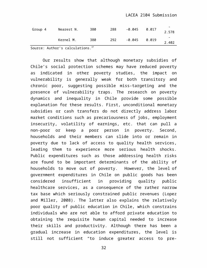
Group 4 Nearest N. 380 288 -0.045 0.017 -2.578Kernel M. 380 292 -0.045 0.019 -2.402


Our results show that although monetary subsidies of Chile’s social protection schemes may have reduced poverty as indicated in other poverty studies, the impact on vulnerability is generally weak for both transitory and chronic poor, suggesting possible miss-targeting and the presence of vulnerability traps. The research on poverty dynamics and inequality in Chile provide some possible explanation for these results. First, unconditional monetary subsidies or cash transfers do not directly address labor market conditions such as precariousness of jobs, employment insecurity, volatility of earnings, etc. that can pull a non-poor or keep a poor person in poverty. Second, households and their members can slide into or remain in poverty due to lack of access to quality health services, leading them to experience more serious health shocks. Public expenditures such as those addressing health risks are found to be important determinants of the ability of households to move out of poverty. However, the level of government expenditures in

20


Chile on public goods has been considered insufficient in providing quality public healthcare services, as a consequence of the rather narrow tax base which seriously constrained public revenues (Lopez and Miller, 2008). The latter also explains the relatively poor quality of public education in Chile, which constrains individuals who are not able to afford private education to obtaining the requisite human capital needed to increase their skills and productivity. Although there has been a gradual increase in education expenditures, the level is still not sufficient “to induce greater access to pre-primary education and good quality of public education… (thereby condemning low-income households)… to under-invest in human capital” (Lopez and Miller, 2008, p. 6).31 As with health shocks, monetary subsidies are inadequate in dealing with education disparities, an important factor in the perpetuation of inequality in Chile.

VI. Concluding remarksUndoubtedly, Chile has experienced remarkable achievements in poverty reduction since its return to democracy in 1990. This success is a result of the combination of high economic growth and provisioning of social protection through a variety of monetary subsidies program. Although Chile has been successful in lowering its poverty rate from 39% to 14% from 1990 to 2006, a large proportion of the population appears to be vulnerable to falling into poverty, thus raising the need to also assess the impact of social protection programs on vulnerability.

Using propensity score matching and average treatment effect on the treated estimations, our results suggest that the impact of the monetary transfers on vulnerability is somewhat mixed. It seems to help lower the vulnerability in some cases but has little or no positive impact on the transient and chronic poor. Our results appear to be robust to the estimation method used (nearest neighbor and kernel methods).

The results presented in this study are suggestive; they illustrate the importance of assessing the effects of economic and social policies and poverty reduction programs on vulnerability and not just poverty. We recommend further research on vulnerability particularly on the existence of so-called ‘vulnerability traps’ that may have been brought about by the deterioration of labor market conditions and persistence of inequality. This however, is beyond the scope of the present study.

31 Lopez and Miller (2008) also shows that Chile is one of the countries that spend the least per student about 50% less than Korea, for example, despite its steady economic growth.

21


ReferencesAbadie, A., Drukker, Leber J. & Imbens, G. (2004). Implementing matching estimators for average treatment effects in Stata. Stata Journal, 4, 290–311.

Agostini, C. & Brown, P. (2011). Cash transfers and poverty reduction in Chile. Journal of Regional Science, 51, 604–625

Agostini, C., Brown, P., & Góngora, D. (2010). Public Finance, Governance, and Cash Transfers in Alleviating Poverty and Inequality in Chile. Public Budgeting & Finance, 30(2), 1-23

Agostini, C., Brown, P. & Góngora, D. (2008). Spatial Distribution of Poverty in Chile. Estudios de Economía, 25(1), 79-110.

Aguilar, O. (2002). Dinámica de la Pobreza: Resultados de la Encuesta Panel 1996-2001, Technical report, MIDEPLAN, Santiago, Chile.

Amemiya, T. (1977). The maximum likelihood estimator and the non-linear three stage least squares estimator in the general nonlinear simultaneous equation model. Econometrica, 45, 955-968.

Arellano, J. (2004). Políticas sociales para el crecimiento con equidad Chile 1990-2002. Serie Estudios Socio/Económicos, 26, Santiago de Chile.

Baulch, B. & Hoddinott, J. (2000). Economic Mobility and Poverty Dynamics in Developing Countries. Journal of Development Studies, 36(6), 1–24.

Bendezú, L., Denis, A., Sánchez, C., Ugalde, P. & Zubizarreta, J. (2007). La Encuesta Panel CASEN: Metodología y Calidad de los Datos Versión 1.0. Report Observatorio Social Universidad Alberto Hurtado.

Becker, S. & Caliendo, M. (2007). Sensitivity analysis for average treatment effects. The Stata Journal, 7(1), 71–83.

Becker, S. & Ichino, A. (2002). Estimation of Average Treatment Effects based on Propensity Scores. The Stata Journal, 2(4), 358-377.

Heinrich C., Maffioli, A & Vázquez, G. (2010). A Primer for Applying Propensity Score Matching. Impact-Evaluation Guidelines Technical Notes No. IDB-TN-161.

22


Bourguignon, F. & Goh, C. (2004). Estimating individual vulnerability to poverty with pseudo-panel data. The World Bank, and DaeIl Kim, Seoul National University. World Bank Policy Research Working Paper 3375.

Bronfman, J. (2010). Measuring vulnerability in Chile using the panel National SocioEconomic Characteristics Survey for 1996-2001-2006.” Working Paper School of Public Affairs, American University. Presented at LACEA 2011 annual meeting, Nov, 2011.

Caliendo, M. & Kopeinig, S. (2005). Some practical guidance for the implementation of propensity score matching. IZA Discussion Paper No. 1588. Bonn, Germany.

Calvo, C. & Dercon, S. (2005). Measuring Individual Vulnerability. Department of Economics discussion paper series. University of Oxford, March.

Castro, R. & Arzola, M. (2008). Determinantes de la Movilidad de la Pobreza en Chile (1996-2006). Instituto Libertad y Desarrollo, Serie Informe Social, 112.

Castro, R. & Kast, F. (2004). Movilidad de la pobreza en Chile. Análisis de la Encuesta Panel 1996 – 2001. Instituto Libertad y Desarrollo, Serie Informe Social, 85.

Chaudhuri, S., Jalan, J. & Suryahadi, A. (2002). Assessing household vulnerability to poverty from cross-sectional data: A methodology and estimates from Indonesia. Columbia University Department of Economics Discussion Paper Series, 0102-52.

Chaudhuri, S. (2003). Assessing vulnerability to poverty: concepts, empirical methods and illustrative examples. Department of Economics Columbia University. Available at: http://info.worldbank.org/etools/docs/library/97185/Keny_0304/Ke_0304/vulnerability-assessment.pdf.

Chronic Poverty Research Centre (2005). The Chronic Poverty Report, 2004–05, Manchester, UK. Available at: http://cprc.abrc.co.uk/pdfs/CPRfinCOMPLETE.pdf.

Clert, C. & Wodon, Q. (2002). The Targeting of Government Programs in Chile: A Quantitative and Qualitative Assessment. Published in: Chile’s High Growth Economy: Poverty and Income Distribution 1987-1998. World Bank Country Study, Washington, DC, 143-166.

Cochran, W. & Rubin, D. (1973). Controlling Bias in Observational Studies: A Review. Sankhya, Series A, 35 (4), 417–446.

23


Contreras, D. (1996). Pobreza y Desigualdad en Chile 1987-1992: Discurso, Metodología y Evidencia empirica. Estudios Públicos, 65, 57-94

Contreras, D. (2003). Poverty and Inequality in a Rapid Growth Economy: Chile 1990-96. Journal of Development Studies, 39(3), 181-200.

Contreras, D., Cooper, R., Hermann, J. & Neilson, C. (2005). ¿Ha sido en crecimiento pro pobre en Chile? Presented at X Congreso Internacional del CLAD sobre la Reforma del Estado y de la Administración Pública, Santiago Chile, October 18-21. Cruces, G., Gasparini, L., Bérgolo, M. & Ham, A. (2010). Vulnerability to Poverty in Latin America. CEDLAS and CONICET, report prepared for the Chronic Poverty Research Centre.

Direccióin de Presupuesto, Gobierno de Chile. Estadísticas de las finanzas públicas, Dipres. Available at: http://www.dipres.gob.cl/

The Economic Commission for Latin America (ECLAC), (2010). Statistical yearbook for Latin America and the Caribbean. United Nations. ISBN 978-92-1-021073-7.

Elbers, C., Lanjouw, J. & Lanjouw, P. (2003). Micro-Level Estimation of Poverty and Inequality.” Econometrica 71(1), 355-364.

Elbers, C. & Gunning, J. (2003). Estimating Vulnerability. Free University, Amsterdam. Paper presented at the conference Staying Poor: Chronic Poverty and Development Policy. University of Manchester April 7-9, 2003.

Günther, I. & Harttgen, K. (2009). Estimating Households Vulnerability to Idiosyncratic and Covariate Shocks: A Novel Method Applied in Madagascar. World Development, 37(7), 1222-1234.

Haughton, J. & Khandker, S. (2009). Handbook on Poverty and Inequality. The World Bank, Washington D.C.

Heckman, J., Ichimura, H., Smith, J. & Todd, P. (1998). Characterizing selection bias using experimental data. Econometrica, 66(5), 1017–1098.

Hoddinott, J. & Quisumbing, A. (2003). Methods for Microeconometric Risk and Vulnerability Assessments. Social Protection Discussion Paper Series No. 0324, The World Bank, Washington D.C.

24


Imai, K., Wang, X. & Kang, W. (2009). Poverty and Vulnerability in rural China: effects of taxation. Chronic Poverty Research Centre, Working paper 156.

Imbens, G. (2004). Nonparametric estimation of average treatment effects under exogeneity: A review. Review of Economics and Statistics, 86(1), 4–29.

Jha, R. Imai, K. & Gaiha, R. (2009). Poverty undernutrition and vulnerability in rural India: public works versus food subsidy. Chronic Poverty Research Centre, Working paper 135.

Kamanou, G. & Morduch, J. (2002). Measuring Vulnerability to Poverty. WIDER discussion paper 2002/58. Helsinki: UNU-WIDER.

Larrañaga, O. (1994). Pobreza, crecimiento y desigualdad: Chile 1987-1992. Revista de Análisis Económico , 9 (2), 69-92.

Leuven, E. & Sianesi. B, (2003). PSMATCH2: Stata module to perform full Mahalanobis and propensity score matching, common support graphing, and covariate imbalance testing. http://ideas.repec.org/c/boc/bocode/s432001.html.

Ligon, E. & Schechter, L. (2003). Measuring vulnerability. The Economic Journal, 113, March.

Mideplan, (2010). Resultados de la Encuesta CASEN 2009. Available at: http://www.ministeriodesarrollosocial.gob.cl/casen2009/RESULTADOS_CASEN_2009.pdf

Neilson, C., Contreras, D., Cooper, R. & Hermann, J. (2008). The Dynamics of Poverty in Chile” Journal of Latin American Studies, 40, 251–273.

Observatorio Social, Unversidad Alberto Hurtado (2007). La encuesta Panel CASEN: Manual de Usuario.

Pizzolitto, G. (2005). Poverty and Inequality in Chile: Methodological Issues and a Literature Review. CEDLAS, Working Papers 0020, CEDLAS, Universidad Nacional de La Plata.

PNUD Chile, (2009). Análisis de la Encuesta Panel CASEN. Programa Equidad, Santiago Chile.

25


Ravallion, M. (2003). Assessing the Poverty Impact of an Assigned Program. Chapter 5 in The Toolkit for Evaluating the Poverty and Distributional Impact of Economic Policies, Washington DC: The World Bank, EDI Development Studies.

Rodriguez, C., Dominguez, P., Undurraga, E., & Zubizarreta, J. (2008). Identificación y características de la población vulnerable: elementos para la introducción del riesgo. Chapter X on Camino al Bicentenario Propuestas para Chile, Pontificia Universidad Católica de Chile.

Rosenbaum, P. & Rubin, D. (1983). The Central Role of the Propensity Score in Observational Studies for Causal Effects. Biometrika, 70(1), 41-55.

Rosenbaum, P. & Rubin, D. (1985). Constructing a control group using multivariate matched sampling methods that incorporate the propensity score. The American Statistician 39, 33–38.

Rubin, D. & Thomas, N. (1992). Characterizing the effect of matching using linear propensity score methods with normal distributions, Biometrika, 79, 797-809.

Scott, C. (2000). Mixed fortunes: A study of poverty mobility among small farm households in Chile, 1968-86. Journal of Development Studies, 36(6), 155-180.

Stallings, B. & Peres, W. (2000). Growth, Employment and Equity, Brookings Institution Press, Washington D.C.

Thomas, T. (2003). A Macro-Level Methodology for Measuring Vulnerability to Poverty, with a Focus on MENA Counties. Paper presented at the Fourth Annual Global Development Conference, Globalization and Equity, Cairo, Egypt, January 21.

Waissbluth, M. (2005). La Reforma del Estado en Chile 1990-2005. Diagnóstico y Propuestas de Futuro. Serie Gestion 76 Santiago: Universidad de Chile, 2005. Available at http://www.dii.uchile.cl/~ceges/publicaciones/ceges76.pdf .

Wooldridge, J. (2002). Econometric Analysis of Cross Section and Panel Data. MIT Press.

You, J. (2010). Evaluating poverty duration and transition: A spell-approach to rural China. BWPI Working paper 134, Forthcoming in Applied Economic Letters, 2011.

Zhang, Y. and Wan, G. (2008). Can We Predict Vulnerability to Poverty? United Nations University UNU-WIDER Research Paper 2008/82.

26

http://www.dii.uchile.cl/~ceges/publicaciones/ceges76.pdf


Zubizarreta, J. (2005). Dinámica de la Pobreza: el Caso de Chile 1996-2001. Unpublished Memoria para optar al título de Ingeniero Civil de Industrias, con Diploma en Ingeniería Matemática, Pontificia Universidad Católica de Chile.

27


Appendix A. Composition of Government Social Expenditure (as a percentage of GDP)

1987 1988 1989 1990 1991 1992 1993 1994 1995 1996 1997 1998 1999 2000 2001 2002 2003 2004 2005 2006 2007 2008 2009

Environment Protection 0 0.1 0 0 0 0 0 0.1 0.1 0.1 0.1 0.1 0.1 0.1 0.1 0.1 0.1 0.1 0.1 0.1 0.1 0.1 0.1

Housing and Community Services

0.2 0.2 0.2 0.2 0.1 0.2 0.2 0.2 0.2 0.2 0.2 0.2 0.3 0.3 0.2 0.2 0.2 0.2 0.2 0.2 0.3 0.3 0.4

Health Services 2 2.1 2 1.9 2 2.2 2.3 2.4 2.3 2.4 2.4 2.6 2.8 2.8 3 3 3 2.8 2.8 3 3 3.3 4

Recreation, Culture and Religion

0.1 0.1 0.1 0.1 0.1 0.1 0.1 0.1 0.1 0.1 0.1 0.1 0.1 0.1 0.1 0.1 0.1 0.1 0.1 0.1 0.1 0.2 0.2

Education 3 2.6 2.4 2.3 2.3 2.4 2.5 2.5 2.5 2.8 2.9 3.3 3.8 3.7 3.9 4 3.9 3.6 3.3 3 3.2 3.9 4.4

Social Protection 10.3 9.3 8.8 8.1 8.2 7.8 7.9 7.5 7 7.3 7 7.4 7.9 7.9 7.9 7.7 7.5 6.6 6.4 5.8 5.7 6.3 7.4

Total Government Social Expenditure

15.6 14.4 13.5 12.6 12.7 12.7 13 12.8 12.2 12.9 12.7 13.7 15 14.9 15.2 15.1 14.8 13.4 12.9 12.2 12.4 14.1 16.5

Source: Estadísticas de las finanzas públicas, Dipres, years 2004 y 2010. Protection of the environment includes: reduction of contamination, protection of biological diversity and landscape and protection of the environment. Health includes: hospital services, public health services and health. Recreation, culture and religion include: recreational and sporting services and cultural services. Education includes: preschool and primary and secondary education, tertiary education, education not definable by level, education auxiliary services and education. Social protection includes: elderly, family and children, unemployment, housing, research and development related to social protection and social protection.

28


Appendix B. Structure of the “Ficha CAS-II” score and weights

Factor Weight Sub factor Weight Variable Weight

Housing 0.26Protection from the environment

0.4 Walls 0.35

Floor 0.35

Roof 0.3

Overcrowding 0.22 People to rooms ratio 1

Sanitation and comfort 0.38 Water 0.35

Sanitation 0.3

Shower/bath 0.35

Education 0.25 Years of education HH head 1

Occupation 0.22Highest occupation category within the couple or HH head

1

Income/Assets 0.27 Income 0.43 Per capita income 1

Housing 0.13 Property of the land 1

House equipment 0.44 Refrigerator 0.5

Heating system 0.5

Source: Larrañaga (2005)

29


Appendix C.List of Monetary Subsidies provided under Social Protection Program “PROTEGE”I. Potable water subsidy (Subsidio de Agua Potable, SAP)

Household receive a monetary subsidy that ranges from 50%, 77% or 100% of their water services monthly bill applicable to a 15 m3 of water consumption. The eligibility criteria are: must be permanent resident of the rural or urban area, must be a tenant, owner or usufruct, have a connection to the potable water system, must be able to meet the payments and present a application to the municipality of residency.

II. Welfare pension (Pension Asistencial, PASIS)

There are three types of pensions provided:

a) Elderly pension: Consists of a non-conditional monetary subsidy for senior citizens (65 years and older), whose monthly household per capita income is lower than 50% of the minimum wage.

b) Disabled aid: Consists of non-conditional monetary subsidy for people between 18 years old to 64 years that have been declare disable by the government medical commissions, whose monthly household per capita income is lower than 50% of the minimum wage.

c) Mentally disabled aid: This is equal to the disabled subsidy but without the age requirement.

III. Unemployment insurance

Unemployment insurance is mandatory in Chile and it covers formal workers under the labor law. This insurance is financed in part by an individual account, paid by the employee, and in part by a solidarity fund composed by payments done by the employer and the government.

IV. Family subsidy (Subsidio Único Familiar, SUF)

This benefit is targeted to pregnant women and people who bear children under the age of 18. In order to receive this subsidy they cannot be recipients of private or public assistance though the pension system. Pregnant women, mothers, children bearing adults, and disable people not receiving PASIS are thus eligible for this subsidy.

30


Appendix D.For the vulnerability regression we estimated vulnerability based on the household head and its household variables. Some household did not report having a household head thus we re-coded as household head those adults reported as spouse or partners for the missing household heads in the sample. This way we were able to incorporate 301, 293 and 250 household for 1996, 2001 and 2006 respectively.

Note on variables used in FGLS regressions: Age represents the household head years of age, age square; Education variable corresponds to the total years of education of the household head; Home ownership equal to one if the family own their dwelling; Labor participation dummies as follow, unemployed correspond to those household heads that are not working but looking actively for a job, two categories of self employed, one with paid workers and one with out paid workers, wage paid employee and domestic servant dummy, the one category left aside is not in the labor force. In terms of household composition we controlled for the household size that corresponds to the total number of members, a dummy for couple households, (meaning that the household head is married or lives with a partner), male headship dummy, number of children below 7 years old in the household, and the ratio of employed to non-employed members in the household. We also control for regional fix-effects (the 3d region is excluded from the regression).

31


Table D1. FGLS Regression Estimates for 1996 log per capita income and income per capita variance, Urban and Rural households.

VARIABLES Urban Urban Rural Rural

in 1996Income per

capitaIncome

VarianceIncome per

capitaIncome

VarianceAge 0.0108 0.0284** 0.0145 0.0426***

(0.0073) (0.0129) (0.0143) (0.0151)Age square 5.41E-05 -0.000314** 4.42E-05 -0.000411***

(0.0001) (0.0001) (0.0001) (0.0002)Education (years) 0.0689*** -0.00255 0.0494*** 0.0248**

(0.0041) (0.0106) (0.0097) (0.0111)Home ownership dummy 0.338*** -0.241** 0.253*** -0.143**

(0.0393) (0.1100) (0.0641) (0.0634)Unemployed -0.772*** 0.237 -0.372 -0.178

(0.1130) (0.2060) (0.2350) (0.1570)Domestic servant worker -0.401*** -0.243** 0.304 -0.434***

(0.0912) (0.1220) (0.1850) (0.1430)Self-empl. w/o paid workers -0.239*** -0.155* 0.0277 -0.116

(0.0538) (0.0939) (0.1310) (0.1210)Self-emp. w/ paid workers 0.326*** -0.09 0.787*** -0.362**

(0.1060) (0.1100) (0.2280) (0.1440)Waged salaried empl. -0.165*** -0.156* -0.0204 -0.302**

(0.0495) (0.0863) (0.1330) (0.1260)Male household head 0.0966** 0.0196 0.211* 0.0355

(0.0398) (0.0583) (0.1100) (0.0958)Couple HH 0.00749 -0.032 -0.195** -0.0293

(0.0417) (0.0568) (0.0984) (0.1140)Single adult HH 0.126** 0.0708 -0.127 -0.0378

(0.0554) (0.0750) (0.1360) (0.1530)Household size -0.0964*** -0.0231 -0.0846*** -0.0705**

(0.0123) (0.0226) (0.0279) (0.0336)Number of young children -0.0675*** -0.0377 -0.092 0.086

(0.0235) (0.0426) (0.0571) (0.0674)Empl. to HH size ratio 0.840*** -0.0161 0.805*** -0.16

(0.0672) (0.1270) (0.1320) (0.1160)7th Region -0.0959 0.0758 0.229** -0.129

(0.0614) (0.0552) (0.1070) (0.1440)8th Region -0.0314 0.0477 -0.0185 -0.093

(0.0555) (0.0508) (0.1100) (0.1510)Metropolitan Reg. 0.257*** 0.104* 0.399*** -0.205

(0.0545) (0.0606) (0.1180) (0.1480)Constant 9.437*** 0.159 9.140*** -0.0939

(0.1820) (0.2660) (0.3450) (0.3170)Observations 2,299 2,042 552 552R-squared 0.465 0.018 0.398 0.082

Source: Author’s calculations using the Panel CASEN 1996-2001-2006. Robust standard errors in parentheses, *** p<0.01, ** p<0.05, * p<0.1

32




in 2001Income per

capitaIncome

VarianceIncome per

capitaIncome

VarianceAge 0.0330*** -0.000276 0.0117 0.00142

(0.0062) (0.0066) (0.0116) (0.0122)Age square -0.000106* -2.48E-05 6.96E-05 -2.08E-05

(0.0001) (0.0001) (0.0001) (0.0001)Education (years) 0.0683*** 0.00507 0.0303*** -0.00385

(0.0035) (0.0038) (0.0081) (0.0078)Home ownership 0.388*** -0.110** 0.310*** -0.0912*

(0.0363) (0.0485) (0.0554) (0.0552)

Unemployed -0.553*** 0.0241 -0.466*** 0.0586

(0.0688) (0.0876) (0.1410) (0.1000)

Domestic servant worker -0.244*** 0.064 -0.217 -0.216**

(0.0898) (0.1060) (0.2030) (0.1020)Self-empl. w/o paid workers -0.169*** -0.0277 0.0168 0.0594

(0.0492) (0.0608) (0.0962) (0.0860)

Self-emp. w/ paid workers 0.322*** -0.130* 0.890*** 0.34

(0.0772) (0.0737) (0.2750) (0.2990)

Waged salaried empl. -0.0403 -0.169*** 0.00438 0.0551

(0.0436) (0.0590) (0.0968) (0.0942)

Male household head 0.0374 0.0451 -0.0267 -0.107

(0.0371) (0.0435) (0.0843) (0.0790)

Couple HH -0.0551 -0.0241 -0.0663 -0.0723

(0.0372) (0.0384) (0.0808) (0.0732)

Single adult HH 0.103** 0.0505 -0.0881 -0.0405

(0.0458) (0.0494) (0.0958) (0.1280)

Household size -0.130*** -0.0358*** -0.106*** -0.0484**

(0.0105) (0.0104) (0.0188) (0.0198)

Number of young children -0.0109 0.103* -0.0306 -0.0623

(0.0424) (0.0560) (0.0739) (0.0665)Empl. to HH size ratio 0.603*** 0.105* 0.572*** 0.153

(0.0523) (0.0570) (0.1060) (0.1090)7th Region -0.0952 -0.16 -0.211** -0.0608

(0.0685) (0.1100) (0.0918) (0.0899)8th Region -0.129** -0.111 -0.216** -0.0481

(0.0653) (0.1110) (0.0946) (0.0919)

Metropolitan Reg. 0.0826 -0.192* 0.0805 -0.171*

(0.0636) (0.1060) (0.1010) (0.0874)Constant 9.199*** 0.757*** 9.969*** 0.659*

(0.1760) (0.2410) (0.3410) (0.3970)Observations 2,547 2,547 635 635R-squared 0.458 0.035 0.389 0.05


33




in 2006Income per

capitaIncome

VarianceIncome per

capitaIncome

VarianceAge 0.0323*** 0.000424 0.0227** 0.0081

-0.00617 -0.00748 -0.0115 -0.0133Age square -0.000103* -3.55E-05 -7.92E-05 -8.10E-05

-5.55E-05 -6.96E-05 -9.62E-05 -0.000108Education (years) 0.0679*** 0.0164*** 0.0422*** 0.00713

-0.00356 -0.00413 -0.00887 -0.00881Home ownership 0.312*** -0.158*** 0.328*** -0.0867

-0.0346 -0.0499 -0.0558 -0.0612Unemployed -0.343*** 0.193 -0.655*** 0.0508

-0.0957 -0.185 -0.19 -0.197Domestic servant worker -0.274*** -0.274*** -0.349 0.0704

-0.0794 -0.0725 -0.213 -0.163Self empl. w/o paid workers -0.141*** -0.0477 0.0423 0.0192

-0.0492 -0.0517 -0.0949 -0.0887Self emp. w/ paid workers 0.410*** 0.0989 0.740*** 0.215

-0.102 -0.105 -0.218 -0.168Waged salaried empl. 0.0354 -0.172*** -0.029 -0.112

-0.0452 -0.0549 -0.0866 -0.0893Male household head -0.0677 0.0991 -0.140* -0.0199

-0.0418 -0.0605 -0.0779 -0.0845Couple HH 0.0903** -0.168*** -0.0795 0.0816

-0.0425 -0.0615 -0.0838 -0.0961Single adult HH 0.147*** 0.0763 -0.071 0.274***

-0.0471 -0.066 -0.0843 -0.0839Household size -0.0680*** -0.0244** -0.103*** 0.0106

-0.0111 -0.0106 -0.0206 -0.0158Number of young children -0.0987 -0.0146 -0.119 -0.000516

-0.062 -0.053 -0.215 -0.114Empl. to HH size ratio 0.648*** -0.0332 0.533*** 0.000674

-0.0506 -0.0589 -0.0922 -0.1037th Region -0.215*** 0.0354 -0.0111 0.0472

-0.0633 -0.0687 -0.0917 -0.1548th Region -0.266*** -0.0336 -0.0825 -0.0629

-0.0574 -0.0617 -0.0918 -0.161Metropolitan Reg. -0.0658 -0.0315 0.272*** -0.0714

-0.0573 -0.0618 -0.104 -0.161Constant 9.253*** 0.640*** 9.905*** 0.0787Observations -0.182 -0.216 -0.384 -0.486R-squared 0.374 0.051 0.328 0.049


Appendix E.

34


Table E1. Mean vulnerability and poverty rate estimates for total population, by groups for 1996, 2001 and 2006 (in percentage).

NPoverty 1996

Vulnerability 1996

Poverty 2001

Vulnerability 2001

Poverty 2006

Vulnerability 2006

Group 1 2191 10.9% 29.0% 9.7% 27.0% 7.1% 42.0%Group 2 1994 24.1% 54.0% 21.5% 43.0% 9.6% 51.0%Group 3 1629 21.5% 45.0% 18.3% 38.0% 12.0% 49.0%Group 4 4473 26.1% 63.0% 28.1% 56.0% 12.9% 53.0%Total 10287 23.6% 49.0% 20.2% 43.0% 10.5% 49.0%

Source: Author’s calculations using the Panel CASEN 1996-2001-2006

Table E2. Mean vulnerability and poverty rate estimates for the transitory poor, by groups for 1996, 2001 and 2006 (in percentage).

NPoverty 1996

Vulnerability 1996

Poverty 2001

Vulnerability 2001

Poverty 2006

Vulnerability 2006



Table E3. Mean vulnerability and poverty rate estimates for the chronic poor, by groups for 1996, 2001 and 2006 (in percentage).

NPoverty 1996

Vulnerability 1996

Poverty 2001

Vulnerability 2001

Poverty 2006

Vulnerability 2006

Group 1 77 100% 96.0% 100% 95.0% 100% 96.0%Group 2 119 100% 73.0% 100% 97.0% 100% 97.0%Group 3 125 100% 94.0% 100% 85.0% 100% 95.0%Group 4 403 100% 97.0% 100% 94.0% 100% 92.0%Total 724 100% 91.0% 100% 93.0% 100% 94.0%


Table E4. Mean high-vulnerability and poverty rate estimates for total population, by groups for 1996, 2001 and 2006 (in percentage).

NPoverty 1996

Vulnerability 1996

Poverty 2001

Vulnerability 2001

Poverty 2006

Vulnerability 2006



35


Table E5. Mean high-vulnerability and poverty rate estimates for the transitory poor, by groups for 1996, 2001 and 2006 (in percentage).

NPoverty 1996

Vulnerability 1996

Poverty 2001

Vulnerability 2001

Poverty 2006

Vulnerability 2006



Table E6. Mean high-vulnerability and poverty rate estimates for the chronic poor, by groups for 1996, 2001 and 2006 (in percentage).

NPoverty 1996

Vulnerability 1996

Poverty 2001

Vulnerability 2001

Poverty 2006

Vulnerability 2006

Group 1 77 100% 69.5% 100% 40.4% 100% 29.5%Group 2 119 100% 54.2% 100% 45.3% 100% 43.5%Group 3 125 100% 64.5% 100% 65.7% 100% 31.8%Group 4 403 100% 90.1% 100% 69.5% 100% 48.6%Total 724 100% 75.1% 100% 60.2% 100% 42.6%

Source: Author’s calculations using the Panel CASEN 1996-2001-2006.

36

€¦ · web viewsince the return to democracy in 1990, chile has pursued a development strategy...

Documents