wedge theory / compound matrices: properties and applications
TRANSCRIPT

REPORT NO: NAWCADPAX--96-220-TR COPY NO. •« <9
WEDGE THEORY / COMPOUND MATRICES: PROPERTIES AND APPLICATIONS
DebraL. Boutin, M.S. Department of Mathematics Cornell University Ithaca, NY 14853
Ronald F. Gleeson, Ph.D. Department of Physics Trenton State College Trenton, NJ 08650
Robert M. Williams, Ph.D. Mission Avionics Technology Dept. (Code 455100R07) Naval Air Systems Team Warminster, PA 18974-5000
2 AUGUST 1996
FINAL REPORT Period Covering June 1995 to August 1996
Approved for Public Release; Distribution is Unlimited.
cn Prepared for OFFICE OF NAVAL RESEARCH 800 N. Quincy Street Arlington, VA 22217
DTIG QüiiLITY IKbPBCTBD I
ro

NAWCADPAX--96-220-TR
PRODUCT ENDORSEMENT- The discussion or instructions con- cerning commercial products herein do not constitute an endorsement by the Government nor do they convey or imply the license or right to use such products.
Reviewed By: / JU^l^ ate: (a)Q>/ 7 (r
Author/COTR
Reviewed By1
Author/COTR
<T, '*/}£
Reviewed By:
Author/COTR
Date: . 2/W6
Released By ■ i^ Level III Manager
Date . jtfL/fc

REPORT DOCUMENTATION PAGE Form Approved
OMB No. 0704-0188
Public reoortinq burden for this collection of information is estimated to average 1 hour per response, including the time for reviewing instructions, searching existing data sources, aathenngand maintaining the data needed, and completing and reviewing the collection of information. Send comments regarding this burden estimate or any other aspect of this collection of information including suggestions for reducing this burden, to Washington Headquarters Services. Directorate for Information Operations and Reports, 1215 Jefferson Davis Highway Suite 1204 Arlington, VA 22202-4302. and to the Office of Management and Budget. Paperwork Reduction Project (0704-0188), Washington, DC 20503.
1. AGENCY USE ONLY (Leave blank) 2. REPORT DATE
2 August 1996 3. REPORT TYPE AND DATES COVERED
June 1995 to August 1996 4. TITLE AND SUBTITLE
WEDGE THEORY /COMPOUND MATRICES: APPLICATIONS
PROPERTIES AND
6. AUTHOR(S)
*Debra Boutin, M.S. **Ronald F. Gleeson, Ph.D.
Robert M. Williams, Ph.D.
5. FUNDING NUMBERS
7. PERFORMING ORGANIZATION NAME(S) AND ADDRESS(ES)
Naval Air Warfare Center Aircraft Division Warminster Code 455100R07 Warminster, PA 18974-0591
8. PERFORMING ORGANIZATION REPORT NUMBER
NAWCADPAX—96-220-TR
9. SPONSORING/MONITORING AGENCY NAME(S) AND ADDRESS(ES)
Office of Naval Research 800 N. Quincy Street Arlington, VA 22217
10. SPONSORING /MONITORING AGENCY REPORT NUMBER
11. SUPPLEMENTARY NOTES
♦Department of Mathematics Cornell University Ithaca, NY 14853
**Department of Physics Trenton State College Trenton, NJ 08650
12a. DISTRIBUTION/AVAILABILITY STATEMENT
Approved for Public Release; Distribution is Unlimited
12b. DISTRIBUTION CODE
13. ABSTRACT (Maximum 200 words)
The Navy utilizes matrices to analyze radar signals to determine the direction and velocity of aircraft. Matrix analysis is also useful in the sonar classification of submarines. One powerful tool for obtaining information about matrices is wedge theory. (The traditional terminology is "compound matrix theory", whereas modern texts speak of "mappings on the exterior algebra".) Wedge theory is a fundamental tool in multilinear algebra with important applications to group representations and tensor analysis. Current research indicates that it may also be useful in analyzing noisy data matrices, but this potential has not yet been fully explored. The purpose of this report is to collect details about wedge theory, in one accessible place, to facilitate future exploration of this topic. First, basic properties of the wedge operation are given along with definitions and examples. Then, an application to calculating the rank of a matrix with noise is considered. Finally, since the basic constructions can now be easily implemented on desktop computer algebra systems, the procedures for several such packages are illustrated.
14. SUBJECT TERMS Wedge theory, exterior algebra, multilinear algebra, compound matrix, matrix rank, computer algebra.
15. NUMBER OF PAGES
44 16. PRICE CODE
17. SECURITY CLASSIFICATION OF REPORT
UNCLASSIFIED
18. SECURITY CLASSIFICATION OF THIS PAGE
UNCLASSIFIED
19. SECURITY CLASSIFICATION OF ABSTRACT
UNCLASSIFIED
20. LIMITATION OF ABSTRACT
UL NSN 7540-01-280-5500 Standard Form 298 (Rev. 2-89)
Prescribed by ANSI Std Z39-18 298-10?

NAWCADPAX--96-220-TR
Table of Contents
Abstract 1
I. Introduction 2
II. Theoretical Background 2
A. Definitions 2
B. Properties of the Wedge Operator 5
C. Eigenvalues of the Wedge Product 8
D. The Characteristic Polynomial of the Wedge Product 9
E. Different Types of Compound Determinants 12
III. Example of Usefulness 18
IV. Conclusion 20
Acknowledgments 20
Appendix A 21
Appendix B 27
Appendix C : 37
References 38

NAWCADPAX-96-220-TR
WEDGE THEORY / COMPOUND MATRICES: PROPERTIES AND APPLICATIONS
Debra L. Boutin, M.S.* Ronald F. Gleeson, Ph.D.
Robert M. Williams, Ph.D.
2 August 1996
ABSTRACT
The Navy utilizes matrices to analyze radar signals to determine the direction and velocity of aircraft. Matrix analysis is also useful in the sonar classification of submarines. One powerful tool for obtaining information about matrices is wedge theory. (The tradi- tional terminology is "compound matrix theory", whereas modern texts speak of "map- pings on the exterior algebra".) Wedge theory is a fundamental tool in multilinear algebra with important applications to group representations and tensor analysis. Current research indicates that it may also be useful in analyzing noisy data matrices, but this potential has not yet been fully explored. The purpose of this report is to collect details about wedge theory, in one accessible place, to facilitate future exploration of this topic. First, basic properties of the wedge operation are given along with definitions and examples. Then, an application to calculating the rank of a matrix with noise is considered. Finally, since the basic constructions can now be easily implemented on desktop computer algebra systems, the procedures for several such packages are illustrated.
Supported by National Defense Science and Engineering Graduate Fellowship.

NAWCADPAX--96-220-TR
I. INTRODUCTION
The Navy utilizes matrices to analyze radar signals to determine the direction and velocity of aircraft. Matrix analysis is also useful in the sonar classification of submarines. The role of matrices in Navy data analysis and a tool for extracting information from these matrices have been discussed in an earlier report (NAWCADWAR-96-21-TR) by Gleeson, Stiller and Williams.
Another tool for squeezing information out of matrices is wedge theory. In the older literature wedge theory is referred to as compound matrix theory. In more modern texts one speaks of mappings on the exterior algebra. Wedge theory appears to have the potential to be quite useful in analyzing noisy data matrices, but this potential has not yet been fully explored. The purpose of this report is to collect details about wedge theory, in one accessible place, to facilitate future exploration of this topic.
The wedge product of a matrix is defined in Section II. Also, certain basic facts and properties of the wedge product are discussed. In addition, the eigenvalues and character- istic equation for the wedge product, along with a method for efficiently computing the coefficients of the characteristic equation, will be considered. Finally, we examine theorems relating to different types of compound determinants.
In Section III we create a rank three 4x4 matrix with noise deliberately added. We then show that the wedge products of this matrix have a proportionally larger nullity than the original matrix. This increased nullity may afford a method for gaining greater sensitivity in determining the effective rank of the matrix.
Tools such as the wedge product have become more feasible with the development of desktop computer algebra software packages. We will show in Appendix A how to produce the wedge products using Maple, Mathematica and Fermat.
II. THEORETICAL BACKGROUND
A. DEFINITIONS
Given a matrix A, our goal is to define AP(A), a matrix whose entries are the p x p minors of A. This matrix has been called the pth "wedge" of A, "compound" of A or "exterior product" of A, depending on the literature. In this paper we shall refer to AP(A) as the pth wedge of A or as the order p wedge of A.
First a little necessary notation.

NAWCADPAX--96-220-TR
Definition: Let A be an n x n matrix whose entry in the ith row and jth column is
denoted by aij.
A =
/fli.i ai,2 ••• ai,n\ «2,1 «2,2 • • • «2,n
\an,i an,2 ••• S»'
Lexicographically ordered p-sets: Fix a number p between 1 and n, inclusive. Consider all possible sets of p distinct numbers between 1 and n. Order the elements of each set by increasing magnitude. Order the sets by increasing magnitude of the first elements, and when the first elements are equal, by increasing magnitude of the second elements, and when the first and second elements are equal, by increasing magnitude of the third elements, etc. That is, order the sets using a lexicographic or dictionary order. Denote these sets by Si, 52,... , S/n\ so that Si < S2 < • • • < S(*y
Example: Let n = 4 andp = 2. Then Si = {1,2}, S2 = {1,3}, S3 = {1,4}, S4 = {2,3}, S5 = {2,4}, S6 = {3,4}.
Definition: Let Aij be the p x p matrix formed by the intersection, in A, of the rows whose numbers are in the set S,- and the columns whose numbers are in the set Sj. That is, Aij is formed by the entries ahik of A where h is an element of Si and k is an element of Sj, maintaining the relative placement of the entries.
Note: The determinant of any p x p submatrix of A is called an order p minor of A, or alternately, a p x p minor of A. This terminology will be used throughout the paper.
Example: Let A be an abstract 4x4 matrix. Letp = 2. Then S2 = {1,3} and S5 = {2,4}, so A2,5 has entries from the intersection of rows 1 and 3 with columns 2 and 4 of A. Thus
(«1,2 «1,4 2,5 , „ 1 03,2 «3,4
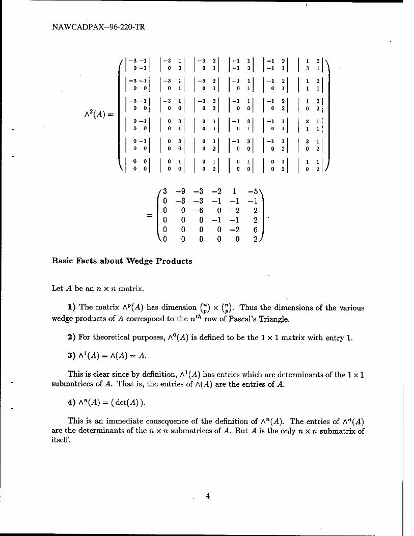
Definition: Let A'(A) be the matrix of size (£) x (J) whose (i, j)th entry is the determinant of the matrix Aij.
-3-1 1 2' 0-131 Example: Let A = I 0 0 x 1 ] • Then,
V 0 0 0 2-
NAWCADPAX-96-220-TR
/
A\A) =
-3 -1 -3 1 -3 2 -1 1 -1 2 1 2 0 -1 0 3 0 1 -1 3 -1 1 3 1
-3 -1 -3 1 -3 2 -1 1 -1 2 1 2 0 0 0 1 0 1 0 1 0 1 1 1
\
-3 -1 -3 1 -3 2 -1 1 -1 2 1 2 0 0 0 0 0 2 0 0 0 2 0 2
0 -1 0 3 0 1 -1 3 -1 1 3 1 0 0 0 1 0 1 0 1 0 1 1 1
0 -1 0 3 0 1 -1 3 -1 1 3 1 0 0 0 0 0 2 0 0 0 2 0 2
0 0 0 1 0 1 0 1 0 1 1 1 0 0 0 0 0 2 0 0 0 2 0 2
(Z -9 -3 -2 1 ~5\
0 -3 -3 -1 -1 -1 0 0 -6 0 -2 2 0 0 0 -1 -1 2 0 0 0 0 -2 6
Vo 0 0 0 0 2/
Basic Facts about Wedge Products
Let A be an n x n matrix.
1) The matrix AP(A) has dimension (£) x (£). Thus the dimensions of the various
wedge products of A correspond to the nth row of Pascal's Triangle.
2) For theoretical purposes, A0(A) is defined to be the lxl matrix with entry 1.
3) AJ(i4) = A(A) = A.
This is clear since by definition, A1 (A) has entries which are determinants of the lxl submatrices of A. That is, the entries of A(A) are the entries of A.
4) An(A) = (det(A)).
This is an immediate consequence of the definition of An(A). The entries of An(A) are the determinants of the nxn submatrices of A. But A is the only n x n submatrix of itself.

NAWCADPAX-96-220-TR
B. PROPERTIES OF THE WEDGE OPERATOR
The beauty and usefulness of the wedge operator is demonstrated in the following properties. A good reference for most of these properties is Determinants and Matrices by A. C. Aitken, [1]. In particular, properties 1), 4), 6), 10) and 11) can be found there. Property 2) can be found in Algebra. Volume 2 by P. M. Cohn, [2].
Theorem: Let A and B be n x n matrices. Let A be a real number. Let I and I' be identity matrices of appropriate dimensions. Then:
Property 1) A*(I) = I'.
This can be seen easily from the definition of AP(A).
Property 2) AP(AB) = A'(A) A' (B).
Example: Let A =
so we can compute A3(AB) =
and B =
2-3 5-6 0-3 3 6 0 0-6 12
. 0 0 0-6
Then AB =
Further, A3 (A) =
A3(£) =
equal to A3(AB).
Now we can compute A3 (A) A3 (B) = which is
Property 3) AP(AA) = A? • AP(A).
In the case A = 1 an easy computation yields AP(AI) = XPI'. If A ^ I, we can write AA = A JA. Using 2), the wedge product becomes AP(AA) = AP(AJA) = AP(AJ) Ap (A) = \pI' Ap (A) = \p Ap (A).
Example: Let A =
A3(2A) =
Then we can compute 2A = liii 0-111 0 0 2 1 0 0 0 3
-16 -8 -8 -16\
0 _204 48 48 ) ' Which Can 6aSily be SGen t0 be 23/v3(A) = 8
0 0 0 -48/
-1 Property 4) (A' (A)) = A^A"1)
NAWCADPAX-96-220-TR
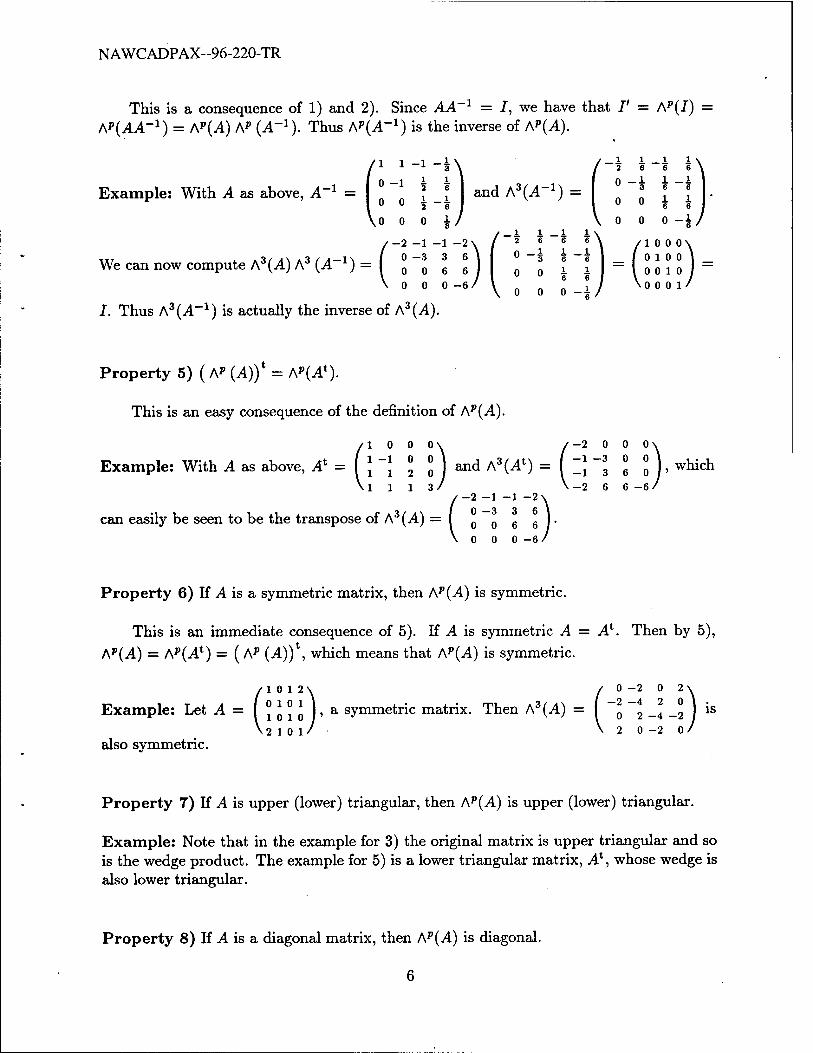
This is a consequence of 1) and 2). Since AA 1 = I, we have that /' = AP(J) AP(AA-1) = AP(A) Ap (A'1). Thus AP(A_1) is the inverse of AP(A).
i l -l -\
Example: With A as above, A-1 = | ° ~* J _J | and A3(A_1) =
We can now compute A3(A) A3 (A 1) =
I. Thus A3(A-1) is actually the inverse of A3(A).
Property 5) ( A' (A))1 = A?(A*).
This is an easy consequence of the definition of AP(A).
(1 0 0 0\ / -2 0 0 0 >
\~\ j o I and A3(^) = ( Z\ 3 6 0 )' wnicn
1113/ V-2 66-6- (-2 -1 -1 -2-
0 0 6 6 0 0 0 -6.
Property 6) If A is a symmetric matrix, then AP(A) is symmetric.
This is an immediate consequence of 5). If A is symmetric A = A1. Then by 5), Ap(A) = Ap(At) = ( AP (A))\ which means that AP(A) is symmetric.
(1012\ / 0 -2 0 2\
loio I' a symmet"c matrix. Then A3 (A) = I ~0 ~2 _4 _2 1 1S
2101/ V20-20/ also symmetric.
Property 7) If A is upper (lower) triangular, then AP(A) is upper (lower) triangular.
Example: Note that in the example for 3) the original matrix is upper triangular and so is the wedge product. The example for 5) is a lower triangular matrix, A*, whose wedge is also lower triangular.
Property 8) If A is a diagonal matrix, then AP(A) is diagonal.
6

NAWCADPAX--96-220-TR
This is an immediate consequence of 7). If A is diagonal matrix, then it is both upper and lower triangular; by 7) so is AP(A).
(1 o o 0\ /6 o o o \
H 1° I . Then A3(A) = f ° o i°2 o ) is dso diagonal. 0004/ \000 24/
Property 9) The complex conjugate of AP(A) is the pth wedge of the complex conjugate of A
(l-t 1 2-t -2t \ /2« 2«' -4« 5-3« \
; »* -> •+*). Th«A'(A) = J f £| -^ ) and 0 0 0-*/ V 0 0 0 1+* /
1 + t 1 2+t 2*
Ä = [ ° 1_i ~x 1~2' ] is the complex conjugate of A. We can then compute ooo«'
-2» -2i 4i 5+3« 0 2« 1-i -1-4« 0 0 1+ 0 0 0 1-«'
A3(A) = ( I 20' }"^ ~1
1"4' ) which is the complex conjugate of A3(A).
Property 10) The Hermitian conjugate of Ap(^4) is the pth wedge of the Hermitian con- jugate of A.
Since the Hermitian conjugate of a matrix is the complex conjugate transposed, this is a straightforward consequence of 9) and 5).
Property 11) (Sylvester) det(A*(A)) = (det(A))^-1^.
Example: In the example for 3), det(A) = -6 while det(A3(A)) = -216 = (-6)®.
Property 12) As a linear operator on a vector space of dimension (£), AP(A) is injective (surjective) if and only if A is injective (surjective) as a linear operator on a vector space of dimension n.
For those who are less familiar with injectivity and surjectivity, we provide the fol- lowing:
A linear operator A is said to be injective if for any two vectors x and y, Ax = Ay only if x = y. That is, no two distinct vectors have the same image under the linear operator.
NAWCADPAX--96-220-TR
A linear operator is said to be surjective if for any vector v there is some vector u so that Au = v. A consequence of A being surjective is that the image of the vector space under the linear operator A is again the whole vector space.
For finite dimensional vector spaces the notions of injectivity, surjectivity and non-zero determinant are equivalent. Thus Property 12) follows from Property 11).
C. EIGENVALUES OF THE WEDGE PRODUCT
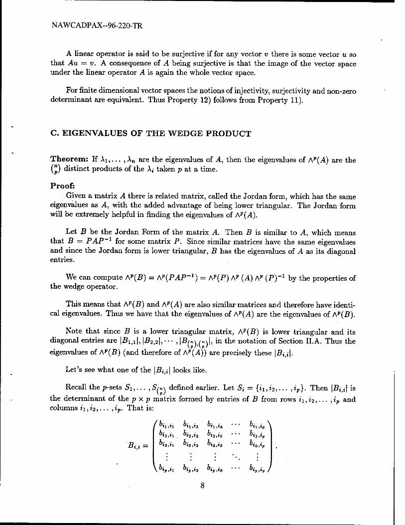
Theorem: If Ai,... , An are the eigenvalues of A, then the eigenvalues of AP(A) are the (") distinct products of the Aj taken p at a time.
Proof: Given a matrix A there is related matrix, called the Jordan form, which has the same
eigenvalues as A, with the added advantage of being lower triangular. The Jordan form will be extremely helpful in finding the eigenvalues of AP(A).
Let B be the Jordan Form of the matrix A. Then B is similar to A, which means that B = PAP"1 for some matrix P. Since similar matrices have the same eigenvalues and since the Jordan form is lower triangular, B has the eigenvalues of A as its diagonal entries.
We can compute AP(P) = A^PAP"1) = AP(P) A* (A) Ap (P)"1 by the properties of the wedge operator.
This means that AP(P) and AP(A) are also similar matrices and therefore have identi- cal eigenvalues. Thus we have that the eigenvalues of AP(A) are the eigenvalues of AP(P).
Note that since B is a lower triangular matrix, AP(B) is lower triangular and its diagonal entries are |Pi,i|, |I?2,2|, • • • , |£/nw„\|, in the notation of Section ILA. Thus the
eigenvalues of AP(P) (and therefore of AP(A)) are precisely these |Pj,j|.
Let's see what one of the |Pi,i| looks like.
Recall the p-sets Si,... ,S/n\ defined earlier. Let Si = {ii,i2,... ,ip}. Then |£,-,,-1 is
the determinant of the p x p matrix formed by entries of B from rows ii,i2,... ,ip and columns ii, i2,... , ip. That is:
Bu = "«2,«'l "«2 >«2 "«2 ,«3 '"' "»2,«p
"»3,«1 "»3, «2 "«3,«3 '" "»3,«p
8

NAWCADPAX--96-220-TR
Since B is a lower triangular matrix, whenever ij < ijt we know that bijyik = 0. In Bi,i this occurs precisely when j < k. Thus £,,, is a lower triangular matrix. Further, since the diagonal entries of B are the eigenvalues of A we know that fetj ti. = A^., the ij eigenvalue of A. Thus,
b
Biti =
0
"«3,»1 "*3>«2
«2,«1
0 0
A «3
V&ip,!! %,t2 °ip,i3
0\ 0 0
Now we can easily compute |5M| = Ait A<a • • • Aip, an eigenvalue of AP(B) and therefore
of A'(A).
Since the eigenvalues of AP(A) are precisely the |£i,i|, which are the products of the eigenvalues of A taken p at a time, the eigenvalues of A'(A) are the (J) distinct products of the A,- taken pat a time.
Example: If A is a 4 x 4 matrix with eigenvalues Ai, A2, A3, A4 then A2 (A) has eigenvalues AiA2, Ai A3, Ai A4, A2A3, A2A4, and A3A4, and A3 (A) has eigenvalues A1A2A3, A1A2A4, A1A3A4 and A2A3A4.
Example: Using the numeric example from Section ILA, we see that A has -3,-1,1 and 2 as its eigenvalues, which implies that A2(A) has eigenvalues -3 • -1 = 3, -3 • 1 = -3 —3 • 2 = —6, -1 • 1 = —1, — 1 • 2 = -2, and 1-2 = 2. We can see immediately that this is true by looking at the upper triangular matrix A2 (A) which we computed.
D. THE CHARACTERISTIC POLYNOMIAL OF THE WEDGE PRODUCT
We would like to be able to find the characteristic coefficients (that is, the coefficients of the characteristic polynomial) of AP(A), directly from the characteristic coefficients of A. This turns out to be a straightforward task for two of the characteristic coefficients.
For the purposes of this paper, the characteristic polynomial of the matrix A is defined to be det(xl - A), though in some literature it is defined as det(A - xl). The polynomials resulting from these two definitions differ by a power of -1. However, we find it convenient to have the highest degree term in the characteristic polynomial be positive, and our definition ensures that.
Let Cfc be the coefficient of the term of degree n-k'm the characteristic polynomial of A. In the characteristic polynomial of AP(A), let dk be the coefficient of the term of degree (J) - k.

NAWCADPAX--96^0^TR
More explicitly, the characteristic polynomial of A will be written as xn + c\xn~l + • • • + cn-\x + cn, while if we let m = ("), the characteristic polynomial of AP(.A) will be written as xm + dix"1-1 -\ 1- dm-\x + dm.
It is a well known fact in linear algebra that in the characteristic polynomial of an n x n matrix, the coefficient of the term of degree n — k is (—l)kSk where Sk is the kth
symmetric function on the eigenvalues of the matrix. That is, Sk is the sum of products of eigenvalues taken k at a time.
So in the characteristic polynomial of AP(A), d\, the coefficient of the term of degree (™) — 1, is (—l)1^!, the negative of the sum of the eigenvalues of AP(A). Since these eigenvalues are products of eigenvalues of A taken pat a time, d\ is, up to sign, actually the pth symmetric function on the eigenvalues of A. Thus:
Theorem: In the characteristic polynomial of AP(A), d\ = (—l)p+1cp.
We now use a similar method to find the constant term, dtn\.
Recall from the properties of the wedge product that det(Ap(A)) = (det(A))^p_1/' and that the constant term of the characteristic polynomial of a matrix is, up to sign, the determinant of the matrix. Thus:
/n-l\
Theorem: In the characteristic polynomial of AP(A), the constant term, d/n\, is (cn)^p_1/', up to sign.
The other characteristic coefficients of AP(A) don't lend themselves to such simple formulae. However, they are still polynomials in the cjt's, and we can actually find them.
Method for Finding Characteristic Coefficients
Let A be an abstract n x n matrix with characteristic polynomial
p{x) = xn + cixn~l H h cn-ix + cn.
Suppose that B is a matrix with the same characteristic polynomial as A. Then the eigenvalues of B, i.e. the roots of the characteristic polynomial, are identical to the eigen- values of A. Thus AP(.A) and AP(JB) also have identical eigenvalues. Since the coefficients of the characteristic polynomial of a matrix are completely determined by its eigenvalues, AP(I?) has the same characteristic polynomial as AP(A).
So what we want is a matrix B, with the same characteristic polynomial as A, whose entries are O's, l's and cjt's. If AP(J5) also has entries of O's, l's and c/t's, the characteristic
10
NAWCADPAX-96-220-TR
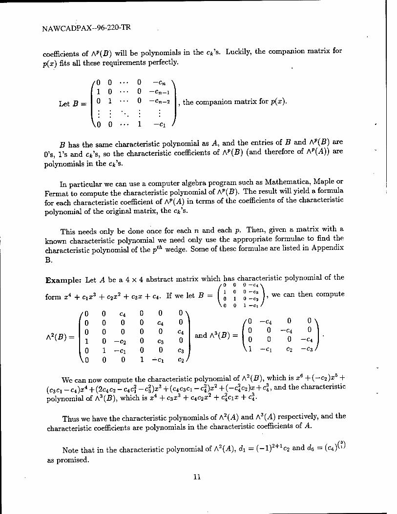
coefficients of AP(B) will be polynomials in the cjt's. Luckily, the companion matrix for p(x) fits all these requirements perfectly.
Let B =
1 0
0 •• 0 •• 1 ••
\0 0 ••
0 0 0
-Cn \ —C„_l
— Cn-2
-ci /
the companion matrix for p(x).
B has the same characteristic polynomial as A, and the entries of B and AP(B) are O's, l's and cjt's, so the characteristic coefficients of AP(B) (and therefore of AP(A)) are
polynomials in the cjt's.
In particular we can use a computer algebra program such as Mathematica, Maple or Fermat to compute the characteristic polynomial of Ap(£). The result will yield a formula for each characteristic coefficient of A* (A) in terms of the coefficients of the characteristic polynomial of the original matrix, the cjt's.
This needs only be done once for each n and each p. Then, given a matrix with a known characteristic polynomial we need only use the appropriate formulae to find the characteristic polynomial of the pth wedge. Some of these formulae are listed in Appendix
B.
Example: Let A be a 4 x 4 abstract matrix which has characteristic polynomial of the
form x4 + cxxz + c2x
2 + c3x + c4. If we let B = , we can then compute
A2(£) =
/° 0 c4 0 0 °\ 0 0 0 0 c4 0 0 0 0 0 0 Ci
1 0 -c2 0 C3 0 0 1 -ci 0 0 cz
\0 0 0 1 -ci 02)
and A3 (5) =
We can now compute the characteristic polynomial of A2(B), which is xe + (-c2)x5 +
(c3ci -C4)x4 + (2c4c2 -Cic\ -4)x3 + (Ciczcx -c\)x2 +{-c\c2)x + c3, and the characteristic polynomial of A3(23), which is x4 + c3x
3 + c4c2x2 + c\cxx + c\.
Thus we have the characteristic polynomials of A2(A) and A3 (A) respectively, and the characteristic coefficients are polynomials in the characteristic coefficients of A.
Note that in the characteristic polynomial of A2(A), dx = (-l)2+1c2 and d6 = (c4)W as promised.
11

NAWCADPAX-96-220-TR
Also, in the characteristic polynomial of A3(A), d\ = (—1)3+1C3 and d^ = (c4)W, again as expected.
Example: Let A be the 4x4 numeric matrix from the example in Section H.A.
The characteristic polynomial of A is x4 + x3 — 7x2 — x + 6, so cx = 1, c2 = —7, cz = —1, and c\ = 6.
Using these in the formulae above, we get that the characteristic polynomial of A2(A) is
x6 + -(-7)x5 + ((-1)(1) - (6))x4 + (2(6)(-7) - (6)(1)2 - (-1) V
+ ((6)(-l)(l) - (6)V + (-(6)2(-7)):r + (6)3
= x6 + 7x5 - 7x4 - 91a;3 - 42x2 + 252x + 216,
and the characteristic polynomial of A3 (A) is
x4 + (-l)x3 + (6)(-7)x2 + (6)2(l)x + (6)3 = x4 - x3 - 42x2 + 36x + 216.
E. DIFFERENT TYPES OF COMPOUND DETERMINANTS
In this section, we cover some results about minors of "compound matrices." The wedge product is one such compound matrix, but there are other compound matrix con- structions different from the wedge product. An excellent reference for this section is, Determinants and Matrices by A. C. Aitken, [1].
Adjugate Wedge Products
Recall that the entries of AP(A) are the order p minors of A. Here we wish to study a matrix, which we will call the pth adjugate wedge of A, whose entries are, up to sign, order n—p minors of A. This new matrix is not quite An~p(A), but it's close. Many of the signs of the entries will be different, and their positions within the matrix will be different. Specifically, we wish the entries of this new matrix to be the cofactors of the minors which comprise Ap(^4). So first we must define what we mean by the cofactor of a minor.
Definition: Let A be an abstract n x n matrix. Let M be the minor which is the determinant of the mxm submatrix obtained from rows r\,... , rm and columns C\,... , cm. Then the complementary minor to M is the determinant of the (n — m)x(n — m) matrix
12

NAWCADPAX-96-220-TR
obtained by deleting rows rx,. M is the complementary minor times (-l)ri+
rm and columns c\,... , cm. + rm+ciH hcm
The cofactor of the minor
' Ol 02 O3 04<
Example: Let A Let M = 02 O3
C2 C3
Mi is 61 64
di d4
6l &2 63 64
C\ C2 C3 C4
di d? ds dt
and the cofactor of M is (_l)2+3+i+3 61 64
d\ di
Then the minor complementary to
= (-1) 61 64 d\ di
Definition Let the pth adjugate wedge of a matrix A, denoted adjP(A), be the (J) x (J)
matrix whose (ij)th entry is the cofactor of the order p minor which is the (j,i)th entry
of A»(A).
Example: Let A =
Then
■ ai 02 03 04 <
61 62 63 64
Cl C2 C3 C4
. d\ 0*2 ({3 <^4 .
/
A3(A) =
Ol 02 03 Ol 02 04 ai 03 04 02 03 04
&1 62 &3 61 62 64 61 63 64 62 f>s t>i
Ci C2 C3 Ci C2 C4 Cl C3 C4 Cl Cz C4
ai 02 03 Ol 02 04 ai 03 04 02 03 O4
6l 62 63 b\ 62 ^4 61 63 64 62 63 &4
di di ds di d2 d4 di dß d4 d2 d3 d4
V
\
Ol 02 03 Ol 02 04 a.\ 03 04 02 03 04
Cl C2 C3 Cl C2 C4 Cl C3 C4 C2 C3 C4
di d2 d3 di d2 d4 di d3 d4 d2 d3 d4
61 62 63 61 62 64 61 63 64 62 t>3 64
Cl C2 C3 Ci C2 C4 Cl C3 C4 C2 C3 C4
di d2 d3 d\ di di di d3 d4 d2 d3 d4
and
adj3(A) =
d4 —C4 64 —04
—d3 C3 —63 03
d2 —C2 62 —«2 1 —di ci —61 01 •
Note that adf(A) is "almost" An~p(A). Up to a factor of (-1),+J, the (i,j)th entry of adf(A) is the (n - 3 + l,n - * + l)th entry of An~P(A). That is, to get ad? (A), we take An~p(A), reflect the entries over the right-leaning diagonal, and adjust the entries by ( — iy+3 = /^n-j+l+n-i+l
Example: Let A =
/4 2-2 1 -5 -2\ '0-2-8-1-4 2 '
0 0 2 0 10 0 0 0-2-8-5
i000021i \0 0 0 0 0-1/
and A3 (A) =
Then we can compute A1 (A) = A, A2(A) =
-4 -16 -10 -9' 0 4 2 1 0 0-2-1 0 0 0-2.
13

NAWCADPAX-96-220-TR
Then adj*(A) =
adj2(A) =
adj3(A) =
-2119 0 -2 -2 -10 0 0 4 16 0 0 0-4
-1-1-5 0 2 2\ 0 2 8 1 4 -5 \ 0 0-2 0-1-1 0 0 0 2 8-2 0 0 0 0 -2 -2 i 0 0 0 0 0 4/
1 4-1-2 0-1-1 0 0 0 2-1 0 0 0 2
has the appropriate relationship with A3(A);
is related in the desired way to A4 2(A) = A2(A); and
is similarly related to A (A) = A
Note: The first adjugate wedge of A, adj*(A) is just called the adjugate of A and is often denoted simply by adj(A). In some literature this is called the classical adjoint of A.
Theorem: (Cauchy) det(adj(A)) = (det(A)) n-l
Example: In the example above, we can easily see that det(A) = —4 while det(adj(A)) = —64 = (—4)4-1 which fits our theorem.
Theorem: A 1 — det(yl) adj(A).
Example: With A as in the example above
dJÄ)*4^"-* -2 1 1 9
0 -2 -2 -10 0 0 4 16 0 0 0 -4
/ k 1 4
1 4 4 \
o 1 1 5 2 2 2
0 0 -1 -4
\ o 0 0 l)
= A -l since
det(A) adj(A) A =
( i
0
1 4 1 2
1 4 1 2
4 ^ 5 2
0 0 -1 -4
\ o 0 0 l)
2 1 0 2\ /i 0 0 0 0 2 1 -M 0 1 0 0 0 0 -1
"4 * ' ° 0 1 0 0 0 0 i/ \0 0 0 1
Theorem: (Jacobi) Let A be a matrix. Then any minor of order r of adj(A) is equal to the cofactor of the corresponding minor in the transpose of A, multiplied by det(A)r_1.
Example: In the previous numeric example, we can see that the minor of adj(A) of order 3, obtained by deleting the last row and last column, is 16. The cofactor of the corresponding minor of the transpose of A is (_i)i+2+3+i+2+3 . i = i. When this is multiplied by det(A)3-1 = (—4)2 we get back the value of the original minor.
14

NAWCADPAX-96-220-TR
Theorem: (Franke) Any minor of order r in the pth wedge of A is equal to the co- factor of corresponding minor in the transpose of the pth adjugate wedge of A, times
(det(^))r"(n'1).
Example: Again let A =
(adjV))'
Then we have A3(A) =
-4 -16 -10 -9' 0 4 2 1 0 0-2-1 0 0 0-2.
and
Consider the order 2 minor of A3 (A) which is the determinant of the matrix obtained -16 -10
4 2
-1 o
from rows 1 and 2 and columns 2 and 3. It is " a" = 8. The cofactor of the
corresponding minor in (adj3^))1 is (-1)1+2+2+3 -i o = (_1)2+3+i+2 . (_2) = _2 We
that det(A) is -4 and 8 = (-2) • (-4)2"(a), as predicted. can see
The Bazin Hybrid
There are more ways of creating new matrices from old ones which result in relation- ships similar to those we saw above. In the following, we discuss Bazin compound matrices and their more general form, Reiss compound matrices, and theorems regarding both.
Definition: Let A and B be n x n matrices. The Bazin hybrid compound of A and B is the n X n matrix whose {i,j)th entry is the determinant of the matrix obtained by replacing column i of A with column j of B.
Example: Let A and B be abstract 2x2 matrices with general entries a,j and bij, respectively. Then the Bazin Hybrid of A and B is
/
V
ftl.1 ai,2 h,2 ai,2 &2,1 02.2 h,2 02,2
«1,1 6l,l «1,1 &1,2
02,1 &2,1 «2,1 &2,2
\
Note: There is no reason to believe that Bazin hybrid of A and B is equal to the Bazin hybrid of B and A. In fact they are not generally equal. So we call the Bazin hybrid of B and A the dual Bazin hybrid of A and B.
Theorem: (Bazin) The determinant of the Bazin hybrid compound of A and B is equal
to (det(A))n-1det(B).
15
NAWCADPAX--96-220-TR
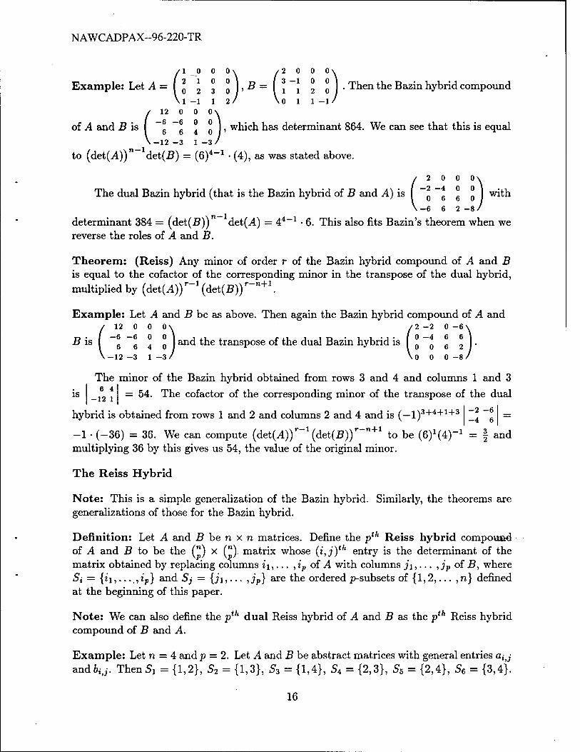
(10 0 0
o 2 3 o I»-^ ~ ( ii 2 o ) ' Then *^e Bazm hybrid compound 1-1 1 2-
(12 o o 0\
6 6 4 o I' wmcn has determinant 864. We can see that this is equal -12 -3 1-3/
to (det(A)) det(B) = (6)4-1 • (4), as was stated above.
(2 o 0 0\
~o ~6 6 o ) w^ -6 6 2-8/
determinant 384 = (det(B)) det(A) = 44_1 • 6. This also fits Bazin's theorem when we reverse the roles of A and B.
Theorem: (Reiss) Any minor of order r of the Bazin hybrid compound of A and B is equal to the cofactor of the corresponding minor in the transpose of the dual hybrid, multiplied by (det(A))r_1 (det(£))r""+1.
Example: Let A and B be as above. Then again the Bazin hybrid compound of A and (12 0 0 0\ /2 -2 0 -6'
~6 ~6 4 o )anc^ ^e transpose of the dual Bazin hybrid is I 0 0 6 2
-12 -3 1-3/ \0 0 0 -8.
is
The minor of the Bazin hybrid obtained from rows 3 and 4 and columns 1 and 3 6 4
-12 1 2 -6
= 54. The cofactor of the corresponding minor of the transpose of the dual
-4 hybrid is obtained from rows 1 and 2 and columns 2 and 4 and is (—1)3+4+1+3
-1 • (-36) = 36. We can compute (det(4))r-1 (det(£))r""+1 to be (6)1(4)"1 = § and multiplying 36 by this gives us 54, the value of the original minor.
The Reiss Hybrid
Note: This is a simple generalization of the Bazin hybrid. Similarly, the theorems are generalizations of those for the Bazin hybrid.
Definition: Let A and B be n x n matrices. Define the pth Reiss hybrid compound of A and B to be the (") x ("). matrix whose (i,j)th entry is the determinant of the matrix obtained by replacing columns ii,... , ip of A with columns ji,... ,jp of B, where Si = {ii,...., ip} and Sj = {ji,... , jp} are the ordered p-subsets of {1,2,... , n} defined at the beginning of this paper.
Note: We can also define the pth dual Reiss hybrid of A and B as the pth Reiss hybrid compound of B and A.
Example: Let n = 4 and p = 2. Let A and B be abstract matrices with general entries a^j aadbij. Then Si = {1,2}, S2 = {1,3}, S3 = {1,4}, S4 = {2,3}, S5 = {2,4}, 56 = {3,4}.
16

NAWCADPAX-96-220-TR
The entry in row 1, column 5 of the second Reiss hybrid of A and B is the determinant of the matrix with columns 1 and 2 of A replaced with columns 2 and 4 of B:
h,2 h,4 «1,3 ai,4
h,2 h,4 0,2,3 GE2,4
&2,3 &3,4 «3,3 G3)4
64,2 &4,4 «4,3 «4,4
Theorem: (Reiss, Picquet) The determinant of the pth Reiss hybrid compound of A
and B is equal to (det(A))("'^(det(B))^Zl^.
Notice that when p = 1 we have the statement of the theorem by Bazin.
Example: Let A and B be as in the previous example. Then the second Reiss /-12 0 0 0 0 0\
' 12 8 0 0 0 0 ' -6 2-6000 0-4 0-4 0 0
-9-1 3-1 3 0 . \ 9 9-3 3 -3 -2 /
hybrid compound is As stated in the theorem, it's determinant
is 13824 = (det(A))^(det(£))^ = 63 • 43.
The dual Reiss hybrid compound is
/
V
-2 0 0 0 0 0 3 3 0 0 0 0 3 1 -4 0 0 0
-3 -3 0 -6 0 0 -9 -1 4 -2 8 0
It's determinant is
0 -6 -12 -12 /
also 13824 = (det(£))^(det(A))^ = 43 : 63.
Theorem: (Reiss, Picquet) Any r x r minor of the pth Reiss hybrid compound is equal to the cofactor of the corresponding minor in the transpose of the dual Reiss hybrid,
multiplied by (det(i4))r"(':il)(det(B))r"(B'^.
Example: Let A and B be as before. Then we need the second Reiss hybrid of A and B
(
\
-12 0 0 0 0 0\ /-2 3 3-3-9 9 12 8 0 0 0 0 \ /031-3-19
-6 2-6000 0-4 0-4 0 0
-9-1 3-1 3 0 9 9-3 3-3-2
, and the transpose of the dual Reiss hybrid
\
\ 0
0 0-404 0 0 0 0-6-2-6 0 0 0 0 8 -12 .
-12/ 0 0 -12-
Consider the minor of the second Reiss hybrid which is the determinant of the matrix obtained from rows and columns 1,2,3 and 4. It's value is -2304. The cofactor of the corresponding minor in the transpose of the dual is (_l)i+2+3+4+i+2+3+4(_96) = _96
Computing (det(A))4"^Z^(det(.B))4"(4;1) yields (6)1 • (4)1 = 24 and multiplying -96 by this gives us —2304, as expected.
17

NAWCADPAX--96-220-TR
III. EXAMPLE OF USEFULNESS
In the earlier report (NAWCADWAR-96-21-TR) by Gleeson, Stiller and Williams it was shown that the characteristic coefficients (cjt's) could.be used to predict the effective rank of a noisy matrix. These coefficients, when properly normalized, fall below predeter- mined threshold values for k greater than the effective rank. These normalized coefficients are called P*'s.
To illustrate how the wedge product could be used in this type of analysis, we create the following matrix:
A =
17.91 28.05 6.45 10.33 -5.97 -11.56 -15.03 -36.72 22.04 33.83 37.56 38.39
.-24.17 -37.40 -17.85 -19.93 >
The matrix A was generated by first creating a rank three 4x4 matrix, and then adding a small random noise contribution to each element. For readability, each element was then rounded to two decimal places. The details of the generation process are spelled out at some length in NAWCADWAR-96-21-TR.
For the matrix A, we have:
Pi = 0.53, P2 = 0.60, P3 = 0.57, 0.09.
The earlier report studied 7x7 matrices with different effective ranks and noise levels. For small noise, the threshold was found to be typically in the range of 0.2 and 0.3. Let us assume that this threshold range does not vary drastically and applies to 4 x 4 matrices. The above distribution of the Pjk's has P3 above the threshold and P4 below the threshold. This is the profile of a matrix whose effective rank is three.
Now let us consider the second wedge of A. The second wedge of A is the following 6x6 matrix:
A2(A)
/-39.57 -230.62 -595.90 -347.01 910.63 -81.47 \ -12.43 530.56 459.88 835.58 727.55 -140.47 8.23 -163.86 -107.32 -259.65 -172.86 55.88 52.85 107.08 580.25 74.30 798.60 802.25 -56.15 -256.63 -768.42 -355.64 -1142.77 -355.87
V -6.64 514.42 488.52 800.76 761.42 -63.36 /
18

NAWCADPAX-96-220-TR
Recall, that if the given matrix A has rank three, then only three of the four eigenvalues are nonzero. With noise added the fourth would also be nonzero, but small compared to the other three. The eigenvalues of the second wedge are equal to the products of A's eigenvalues taken two at a time, so there are (J) or three significant eigenvalues in A2(A). With three significant eigenvalues, A2 (A) should appear to have effective rank three.
The Pjt's for the A2 (A) are the following:
Pi =0.60, P2 = 0.56, P3 = 0.57, P4 = 0.22, P5 = 0.13, P6 = 0.09.
Assuming that the 7 x 7 thresholds work for 6 x 6 matrices, P5 and P6 clearly fall below the threshold range. P4 is on the border; whereas, P3 is higher than the threshold range. This profile indicates that A2(A) is either rank three or four. Actually, the fact that P6 is lower than the threshold, alone implies that the rank of A is very likely less than four. Moreover, when we see that P5 is also less than the threshold, the likelihood of the rank of A being less than four is amplified. Finally, P3 is greater than the threshold. This implies that the rank of A2(A) is at least three. This, in turn, implies that the rank of A itself is three. The main point here is that A2 (A) has more coefficients with which to work and has greater nullity. Using the normalized characteristic coefficients of A2 (A) should give us a greater handle and enhanced sensitivity in determining the rank of the matrix A.
As discussed in Section II, it is not necessary to actually compute A2(A) to determine its Pjt's. All one needs are the characteristic coefficients of A2(A) , and these can be computed in terms of polynomials in the characteristic coefficients of A. A few examples of these polynomials are included in Appendix B.
19

NAWCADPAX--96-220-TR
IV. CONCLUSION
This report may be regarded as a primer on the theory of wedge products.
In Section II we have brought together definitions, properties and theorems relating to the wedge product. Also, we have discussed how the companion matrix can be used to compute the coefficients of the characteristic polynomials of the various wedge products. Finally, theorems which relate to other forms of compound matrices have been explained.
In Section III we have illustrated how the wedge product has the potential to be useful in the determination of the effective rank of a noisy data matrix.
Future work in this area includes determining quantitatively the extent of this po- tential for predicting the effective rank. That is, we should determine whether or not the normalized coefficients of the characteristic polynomial of A2 (A) axe more successful than those of A in finding effective rank. Characteristic coefficients for higher order wedge products should also be studied. Ultimately, the order(s) of the wedge product(s) that optimize results and computation speed should be compared with existing methods for predicting effective rank.
ACKNOWLEDGMENTS
This work was supported by the Office of Naval Research. The authors are especially indebted to Michael Hirsch for writing Appendices A and C, arid carrying out many of the computations in Appendix B. In addition, Michael Hirsch and Frank Grosshans made numerous valuable suggestions which improved the report. We also wish to thank Sueli Rojas for her diligence in typing Appendix B, and George Nakos for writing the Maple program for computing the wedge product listed in Appendix A. Aj\4S-Tgfi. was used in the preparation of this report.
20

NAWCADPAX--96-220-TR
APPENDIX A
SAMPLE RUN SESSIONS
Here we have included sample code that illustrates the syntax for evaluating wedges of matrices on three different mathematical software packages: Maple (version 5, release 3.0), Mathematica (version 2.2), and Fermat (version 1.1). In the symbolic examples below WA2 is the second order wedge of matrix A.
Maple
In Maple, there is a wedge product function (&") in the differential forms library. Unfortunately, the intent of this function was for differential forms, not for linear algebra. The wedge product command does not work on all matrices; specifically, it may fail on matrices containing zero entries. This would put limitations on the number of matrices for which the Navy could find the wedge product. In light of this, George Nakos has written a program using Maple syntax that computes the wedge product of any matrix. This file can be written in any text editor. Maple can access this file with the command 'read < filename >; '. The program is as follows:
with(linalg): with(combinat,cartprod):
#This function takes a list of lists [[a, 6,...], [al,61,...],... #and computes the Cartesian product [a,b,...] x [al,61,...] x ... lesslistsO := proc(lis) local 11,car;
11.:- []; car := carprod(lis); while not car[finished] do
11 := [op(ll),car[nextvalue] ()] od: RETURN(11); end:
# This function takes a list of numbers and returns a list of lists #of numbers with entries < to the ^corresponding entries of the original. For example, #Lesslists([2,4,3]); yields [1,1,1], [1,1,2],..., [2,4,3] Lesslists := proc(lis)
local ll,i,n;
11 := []; for i from 1 to nops(lis) do 11 := [op(ll),[$l..lis[i]]]:
od:
21

NAWCADPAX--96-220-TR
11 := lesslistsO(ll);
RETURN(11); end:
#This function tests whether the length of f is n
lengthNQ : = proc(f,n) evalb(nops(f) = n) end:
# From a list lis, pick the elements of length n PickLengthN : = proc(lis,n) select (lengthNQ,lis,n) end:
#This function deletes repeated elements in a list
DeleteRepeated := proc(lis)
local 11,i; for i from 2 to nops(lis) do
if evalb(not member(lis[i] ,11)) then 11 := [op(ll),lis[i]];fi:
od: RETURN(11); end:
# This function takes two >0 integers n and k, n > k, and returns all pairs
#of the form (i,j) with i < j and i < k and j < n.
Submatrixlndex := proc(n,k) local tt; tt:= [$(n-k+l)..n]; LessLists(tt); map(convert,",set); PickLengthN(",k); DeleteRepeatedC); tt := map(convert,",list);
Return(tt); end:
# This function takes a list of numbers and returns the ^complete Cartesian product of the element lists
ListOfPairs := proc(lis) local ll,nn,i,j; nn := nops(lis); for i from 1 to nn do
for j from 1 to nn do 11 := [op(ll),[lis[i],lis[j]]];
od: od:
22

NAWCADPAX-96-220-TR
RETURN(11); end:
# MAIN FUNCTION. Computes the k x k minors of matrix A Minors := proc(A,k)
local n,dimmat,kk,11,i; n :- vectdim(rov(A,l)); Submatrixlndex(n,k);
dimmat := nops("); kk := ListOfPairs("");
11 := □; for i from 1 to nops(kk) do
11 := [op(ll),det(submatrix(A,op(kk[i])))]; od:
RETURN(matrix(dimmat,dimmat,11)); end:
Example:
(a\ a2 o3 o4 ' 61 62 63 64 j Qne wouJ^ cl c2 c3 c4 ■ '
,.„,„.., dl d.2 dZ di read in the above tile and then type: > A := matrix(3,3, [al, a2, a3, a4,61,62,63,64, cl, c2, c3, c4, dl, d2, d3, d4]); > WA2 := M«noT5(i4,2);
The output to this would be the following matrix:
ol62-o26l al63-a36l ol64-a46l o263-a362 a264-a462 a364-a463 alc2-o2cl alc3-a3cl aid—aid a2c3-a3c2 a2c4-a4c2 a3c4-o4c3
■KXTAO •— I old2-o2dl olrf3-a3<fl ald4-a4d\ a2d3-a3d2 a2d4-a4d2 a3d4-a4d3 61c2-62cl 61c3-63cl 6lc4-64cl 62c3-63c2 62c4-64c2 63c4-64c3 b\d2-b2dl b\d3-b3d\ 6ld4-64dl 62<f3-63<*2 62d4-64d2 63d4-64d3 cld2-c2d\ c\d3-c3dl cld4-c4dl c2d3-c3d2 c2d4-c4d2 c3d4-c4d3
Mathematica
Mathematica has a built in command for computing the wedge product, namely "Minors[A,p]". This command takes two parameters; the first is the name of the matrix, and the second is a positive integer denoting the order of the wedge.
Example :
23

NAWCADPAX--96-220-TR
As in the previous example, if we wish to compute the second wedge of a 4 x 4 matrix in Mathematica, we would enter:
A = {{<zl, a2, a3, a4}, {ab, a6, a7, a8}, {a9, alO, all, al2}, {al3, al4, al5, al6} } WA2= Minors[A,2]
Fermat
Fermat is a mathematical software system written by Robert Lewis. While there is no built-in function for computing the wedge product, there will be soon. Michael Hirsch has written a program in the Fermat language that can be used in the absence of a wedge product function. Run times are faster than Mathematica and Maple for large symbolic matrices. Once the code is within the Fermat shell, run times using Fermat should be even shorter than they are currently (using the Hirsch program).
;This is the main function for the program :Wedge(p,d,matrix2; m,n,i) =
:cols = Cols[p]; :rows = Deg[p]/cols; :n = Q (cols.d); :m = C (rows,d); :ri « 0; :ci = 0; :b[m,n]; :x[d]; :y[d]; :temp[d,d]; Genr(rows,d,l,l); :[b] = ™ [b];
ID [temp] ; : [matrix2] = [b] ; «D>3; 0.;
;This function generates all of the possible row combinations
;for the wedge :Genr(m,dd,j,s;i)=
if (dd = 0) then (:ri+; :ci =0; Genc(cols,d,l,l) )
else ( for ( :i=s,m+l-dd) do
24

NAWCADPAX-96-220-TR
( :x[j] = i; - Genr(m, dd-1, j+1, i+1 );
) ).;
;This function generates all of the possible ;column combinations for the wedge :Genc(n,dc,k,l;i)- if (dc = 0)
then (:ci+; Dump(ri,ci) ) else ( for ( :i=l,n+l-dc) do
( :yCk] = i; Genc(n, dc-1, k+1, i+1 );
)
).;
;This function calculates the determinant of each ;submatrix for the entries of the wedge :Dump(row,col; q,w) =
:temp[d,d] ; for( :q=l, d ) do
( for( :w=l,d )) do ( :temp[q,w] = p[x[q],y[w]] )
( ); :b [col, row] = Det[temp];
<D [temp] .;
After reading this program into Fermat, using the wedge function is easy. Just type the following:
> Wedge(matrixl ,d,matrix2)
where matrixl is the original matrix, d is the order of the wedge, and matrix2 is the variable that will be assigned to the wedge.
Example:
In Fermat to compute the second wedge of a 4 x 4, we would enter:
>:a[4,4] >: [a] = [[al,a2, aZ, aA, „
a5,a6,a7,a8, „ a9,al0,all,al2, „ al3,al4,al5,al6]]
25

NAWCADPAX-96-220-TR
>:IüO2[6,6]
>Wedge([a],2,[wa2])
26

NAWCADPAX-96-220-TR
APPENDIX B:
CHARACTERISTIC COEFFICIENT RELATIONSHIPS
This Appendix contains a few sample coefficients of the characteristic polynomial of the wedge products (d^s) expressed as polynomials in the coefficients of the characteristic polynomial (cjfc's) of the given matrix (A).
If A is a 3 x 3 matrix:
For A2(A):
di = -c2
di = C1C3
d3 = -c\
For A3(A):
di = c3
If A is a 4 x 4 matrix:
For A2(A):
d\ = -c2
di = ci C3 — C4
dz = 2c2C4 — CjC4 — c3
C?4 = C1C3C4 — c\
d5 = -c2c\
d6 = c|
27

NAWCADPAX--96-220-TR
4x4 matrix cont.
For A3(A):
d\ = c3
C?2 = C2C4
d3 = CiC^
d4 = c\
For A4 (A):
d\ = —C\
If >1 is a 5 x 5 matrix:
For A2 (A):
d\ = -c2
d2 = C1C3 — C4
dz = C1C5 + 2c2c4 - cfc4 - c? 3
3„ „2 ^4 = C3C5 - 3cic2c5 + c\c5 — cz + C1C3C4
d5 = -c2c| - cf C3C5 + 2c2c3c5 + 2cic4c5 - 2c\
d& = c| + cic2c4c5 - 3c3c4c5 - cf c\ + c2c\
d-i = C4C2, + 1cxczc\ - c\cl - cic\cr,
d$ = c2c4ci? - c\c\
d9 = -czc\
d\o = c\
28
NAWCADPAX-96-220-TR
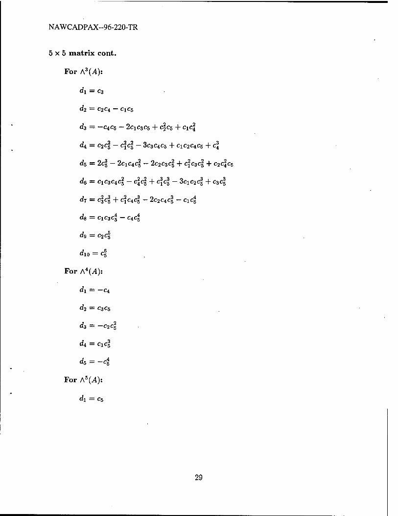
5x5 matrix cont.
For A3(A):
d\ — c3
C?2 = C2C4 — C1C5
^3 = -C4C5 - 2ciC3C5 + C2C5 + Cic|
d4 = C2C§ - cf ci? - 3c3C4C5 + C1C2C4C5 + c3
ofe = 2c| - 2cic4c| - 2c2c3cf + c?c3c|? + 02^05
d6 = ciCsCicj - c\c\ + c\c\ - Zcic2c\ + czc\
dr = 44 + 4C*4 ~ 2c2c4c| - cic|
<*8 = C1C3C5 - C4c|
dg = c2c|
c?io = 4
For A4(4):
c?i = —C4
^2 = C3C5
<f3 = -C24
d4 = ci4
da = -c4
For A5 (A):
d\ = c5
29

NAWCADPAX--96-220-TR
If A is a 6 x 6 matrixr
For A2(A):
d\ = —c2
d2 = C\c% — c4
dz = -c\ - cjci + 2c2c4 + C1C5 - c6
d4 = C1C3C4 - c\ + c\c5 - 3cic2c5 + C3C5 - c\c6 + 2c2c6
d5 = -c2c\ - clczc5 + 2c2c3c5 + 2cic4c5 - 2cj
-cjc6 + 4cf c2c6 - 2c2c6 - 3cic3c6 + 2c4c6
d6 = c\ + C1C2C4C5 - 3c3c4c5 - 44 +c2cl
+clc3c6 - 3cic2c3c6 + 3c|c6 - cf c4c6 + 3cic5c6 - 2c\
d7 = -cic\c5 - 44 + 2cic3cl + c4cl - c\c2cAc6
+2c^c4c6 + C1C3C4C6 - c\ca + cfc5C6 - cic2c5c6
-3c3c5c6 - cjcj?
d8 = c2c4cl - cic| + cjcjce - 2c2c\c& + cic\cbc6
9 O 9 -2CJC3C5C6 - C2C3C5C6 + C1C4C5C6 + C5C6 - C^Cg
+44 + 3cic3cl
d9 = -c3cl - cic2c4c5C6 + 3c4c5c6 + cjclc6 + c2c\c&
-44 + 3cic2c3ci - Zcjcl - c\c4c\ - 3cic5ci + 2c\
d10 = 4 + ciczc\c& - 4cAc2
5c6 + cjc4cl - 2cic3c4cl + 2c\c\
-2cxc2chc\ + 3c3c5ci + 2c\c\ - 2c2c\
d\\ = -cic|c6 - c2c3c5cl + 3cic4c5cl + 44 + 44
-C1C3CJ? - 2c44
d\2 = C244 + C14 ~ 2C2C4C| - C!C54 + 4
du = c24 - C3C5C6
d14 = c44
30

NAWCADPAX--96-220-TR
6x6 matrix cont.
For A2(A):
d15 = -c\
For A3(A):
d\ = c3
d2 = C2C4 — C1C5 + C6
d3 = C1C4 + C2C5 — 2C1C3C5 — C4C5 — C1C2C6 + 3C3C6
^4 = c\ + C1C2C4C5 - 3c3C4C5 - c\c\ + C2c\ + c\c&
—3C1C2C3C6 + 3c|c6 + c\ciCs — C2C4C6 + C1C5C6
^5 = c2clc5 + cf c3c\ - 2c2c3c\ - 2cic4c| + 2c\
+C1C2C4C6 — 2c\c3C±C§ — C2C3C4C6 + 3ciC4C6 — 2c\c2C^C&
+3c2!c5c6 + 2cic3c5c6 - 4c4c5c6 + 2cf c| - 4cic2c|
+3c3c2
^6 = C1C3C4CI - ac\ + c\c\ - Zc\c2c\ + C3c\
+C2C4C6 - 2C1C3C4C6 + 2C4C6 + C1C2C3C5C6 - 2c\c3C5C6
—C1C3C5C6 — 3C1C4C5C6 + 6C1C2C4C5C6 — 2C3C4C5C6 + Ac2c\c$
-cjcjcj + 2c\c\ + c\c3c\ - 2cic2c3cl + 3c|c|
+4c^c4c2
i - 8c2c4cl - 4cic5c| + 3c|
d7 = c?,«:3; + cf C4C3; - 2c2c4c| - c^l + cic2c3c4c5ce
-3cfc4c5C6 - 3cfc|c5c6 + 5c2c|c5c6 + clc2clc6 - 3ciclclc6
-clc3clc6 + C2C3C2iC6 + 4C!C4C|C6 + cfce + cf C2,^
—Zc\c2c\c\ + 3C3CI — 2c\c2c±c\ + 5C1C2C4C6 + cf C3C4CQ
—5c2c3C4cl + cic\c\ - c\c5cl + Ac\c2csc\
+c\c5c\ - C!C3c5cl - 6ctc5cl + c\c\ - §c\c2c\
+3c34
31
NAWCADPAX-96-220-TR
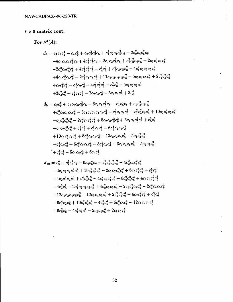
6x6 matrix cont.
For A3(A):
d& = cic3c| - cAc\ + c244c6 + c\c2Ciclc& - 2clc4clc6
-AciC3c4clc6 + Acl4c6 - 2c!C2clc6 + c\c\c±c\ - 1c2c\c±c\
-2c\c2c\cl + ±444 - 44 + c\c3c54 - Ac\c2c3chcl
+4cic|c5c^ - 2c\cAcbcl + IIC1C2C4C5CJ? - 5c3c4c5c| + 2c\44
+c244 - c\c2c\ + ±444 - c\c\ - hcic2c3c\
+344 + c\cAc\ - 7c2ci4 ~ Seiest + 34
dg = C24 + ClC2C34c6 - 6c2C4c|c6 - C1C5C6 + C1C3C5C6
+4c3CiC54 - 5cic2c3c4c54 - 4c*c5cl - 44c$4 + I0c24c54
-Cx44c\ - 24c344 + 5C2C344 + 6C!C444 + 44
-c!c244 + 44 + 4c*4 - 6ci c2°*4
+10cic^c4c3
5 + bc\c3Ci4 - 10c2c3c44 - 5ci44
-c\c54 + 6c?c2c5c| - 5c|c5c| - 3cic3c54 ~ 5c4c5c|
' +44 - 5cic2Ce + 6c3c£
d10 = 4 + 44ce - 6c4c^c6 + 4444 - ±4c*44
-2cxc3cA44 +10444 - 2ciC2cgc| + 6c344 + 44
-Ac24ci4 + 444 - ^4^44 + $444 + ^i^44
-444 ~ 24c2c3c54 + 4:4c3C54 - 2c^4^4 - 2cf c4c5c|
+ 12ciC2C4C5c| - 12c3c4c54 + 2444 ~ ^i44 + 44
-64c24 +10444 - ±44 + §4c*4 - i2cic2c34
+Q44 - 44c*4 - 2c2C4cg + 2cic5c|
32

NAWCADPAX--96-220-TR
6x6 matrix cont.
For A3(A):
dn = c2c\c6 + cic2c3cfcj? - 6c2c444 - cx44 + cidjc5c|
+4c3c4c54 - hcic2c3c4c*,4 - 4c4cs4 - c\c\c5cl + 10c2clc5cl
-Ci4cl4 ~ 1c\csclc\ + 5c2c3c2
54 + 6cic4c2c3
+44 - cxc2c\c\ + 44 + 4C*4 - 6c?c2c4c£
+10cic^c4c| + 5c^c3c4c| - 10c2c3c4C6 - 50x44 - 4C$4
+6c?c2c5c| - 5c^c5c| - 3cic3c5c| - 5c4c5c| + cf 4
-5cic2Cß + 6c3c|
^i2 = c!c344 - ^44 + ^444 + c\c2cA44 - 24^44
-4^03^44 + ±444 - 2cxc244 + C\4CA4 - ^4^4
-24c244 + ±444 - 44 + CiC3C5c| - A4C2C3C54
+4cic|c5c| - 2cfc4c5c| + llcic2c4c5c| - 5c3c4c5c| + 2c\44
+c244 - 4^4 + ±444 - 44 - 5cxc2c3c|
+344 + 4c*4 - 7c2c44 - 5clC5c| + 34
di3 = 444 + 4c*44 - 2c2c444 - cx44 + cic2c3c4c54
-34cic54 - 344c54 + 5c24c54 + 4^44 - 3^444
-4^44 + c2c344 + 4clC444 + 44 + 444
-3cxc244 + 344 - 24c2c*4 + 5c!4c44 + 4c3c*4
-5c2c3c4c| + ci44 - 4^4 + ±4 c2c54 + 4c$4 - cic3c54
-6c4c54 + 44 - 6clC24 + 3c34
du = cic3c444 - 444 + 444 - 3cic244 + c344
+444 - 2clC344 + 244 + 4c2c3c54 - i4c*c$4
-c\4c$4 - 3c?c4c5c| + 6cic2c4c54 - 2c3c4c54 + ±c244
-444 + 244 + 4c34 - 2clC2c34 + 344
+44c44 - Sc2c44 - Acxc54 + 34
33
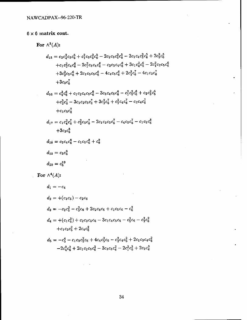
NAWCADPAX--96-220-TR
6x6 matrix cont.
For A3(A):
di5 = c2c2
4c54 + c\c3cl4 - 2c2c3cl4 - 2clCi44 + 244
+cxc\cA4 ~ 2c\czc±4 ~ C2C3C4C6 + %cic\4 ~ 2c\c2c$4
+3c|c5c| + 2dc3c54 ~ 4c4(*4 + 2cic6 - 4cic2cJ
+3c3cJ
<*16 = 44 + C!C2C4C54 ~ 3c3C4C5C^ - c\44 + C2C14
+44 - 3ciC2C3cJ + 344 + C1C4C6 - C2C*4
+cic54
dn = ci44 + C2C5C6 _ 2cic3c5cJ - c4c54 - cic2cj?
+3c3c|
^18 = C2C4c| - CiC5c| + 4
dig = Cz4
d20 = 4°
For A4(A):
d\ = —C4
^2 = +(C3C5) - C2C6
dz — -c24 - 4ce + 2c2c4c6 + cic5c6 - c|
^4 = +(ciCg) + c2c3c5c6 - 3cic4c5c6 - Cj?C6 - C^Cg
+dc3c| + 2c4c|
d5 = -cf, - cic3c|c6 + 4c4c§c6 - c|c4c| + 2cic3c44
-244 + 2clC2c54 - 3c3c5cg - 2c\4 + 2c24
34

NAWCADPAX-96-220-TR
6x6 matrix cont.
For A4 (A):
de = +(c3ci?c6) + C-LC2CIC*,CI - 3c3c4c5cjj - 4clcl - c244
+44 - 3cic2c3c| + Zc\4 + c\ci4 + 3cic5c^ - 2c,
d7 = -c2c4cl4 + ci44 - 444 + 2c244 - ci4<*4
+2cf c3c5c| + C2C3C54 - cic4c5c| - 44 + 4c*ci
~C2C6 — 3cjC3Cg
ds = +(ci4c54) + C2C5C6 _ 2ciC3c|c^ - C^\4 + 4C2C4C6
-2c^C4c| - C1C3C4C6 + C4CI - cf c54 + cic2c5c|
+3c3c5c£ + 44
dg = —4ci ~ cic2C4c5c| + 3c3c4c5c| + c?ci?c| - c244
-Cic3c| + 3ciC2C3c| - $44 + cfece - 3cic5c|
dio = +(c2C4c|) + 4czcs4 - 2c2c3c5c| - 2cic4c54 + 2c|c|
+cf 4 - 4cf c2c^ + 2c^ + 3ciC3c^ - 2c4c|
d\\ = -cic3c4c| + 44 ~ 4cs4 + 3cic2c5c£ - c3c54
+c?4 - 2c2c£
di2 = +(c§4) + 4c*cl ~ 2c2C4cJ - cic54 + c§
^13 = -ClC3c| + C44
du = +(c24)
<*i5 = -4°
For A5(A):
d\ = c5
C?2 = C4Cß
«fo = C3Cg
35

NAWCADPAX--96-220-TR
6x6 matrix cont.
For A5 (A):
d4 - c2c\
dh = cic|
d6 = 4
For A6(A):
d\ = C6
36

NAWCADPAX-96-220-TR
APPENDIX C
dk DEPENDENCE
As mentioned in Section II D, one can find the djt's by looking at the characteristic polynomial of the pth wedge of the companion matrix for a given polynomial. Appendix B specifies how the c^'s and d*'s are related. But how are the d^s related to each other? Although the cjt's are algebraically independent, the djt's are not. Below is code from Mathematica which uses the Gröbner basis tool to calculate the dk relations. The Gröbner basis tool was applied to the equations from Appendix B using the second wedge of a 4 x 4 matrix. Recall from Appendix B, that the second order wedge of the 4x4 matrix has six «fit's. In the ideal generated by this tool, there are five polynomials that only involve the six djt's. By setting these polynomials equal to zero and simplifying we get five useful dk relations.
GroebnerBasis[{dl + c2,
d2 + c4-cl* c3,
d3 + c4 * clÄ2 + c3~2 - 2c2 * c4,
d4 + c4~2 - cl * c3 * c4,
d5 + c2*c4~2,
d6 - c4"3},
{el, c2, c3, o4, dl, d2, d3, d4, d5, <Z6}]
The output to this command is a Gröbner basis. The first five polynomials in the basis, however, depend only on the d^s. They are as follows:
d23dQ-d43, dld42 - d22d5, dld2d6 - d4d5, dl2d4d6-d2d52, dl3d62-d&.
Setting each of these equations equal to zero and reducing them provides a way of examin- ing the relations between the d^s. In fact, for this example, it turns out that the equations reduce to the following:
d5 = d\ * do1'3
d4 = d2*d62'3.
Hence, this gives us an easier way to calculate the d^s.
37

NAWCADPAX--96-220-TR
References
1. Aitken, A.C., Determinants and Matrices, pp.101 to 103, Oliver and Boyd, Edinburgh, 1939.
2. Cohn, P.M., Algebra. Volume 2. p.78, John Wiley k Sons Ltd., New York, 1977.
3. Doolin, B.F., and Martin, C.G., Introduction to Differential Geometry for Engineers. pp.71 to 84, Marcel Dekker, Inc., New York, 1990.
4. Turnball, H.W., The Theory of Determinants. Matrices, and Invariants, pp.107 to 109, Dover, New York, 1960.
38

Distribution List Report No. NAWCADPAX- -96 - 220 - TR
No. of Copies Office of Naval Research 2 800 N. Quincy St. Arlington, VA 22217 Marine Corps Research Center 2040 Broadway Street Quantico, VA 22134-5107
Marine Corps University Libraries 2 Naval Air Systems Command Air-5002 Washington, DC 20641-5004
Technical Information & Reference Center 2 Naval Air Warfare Center, Aircraft Division Building 407 Patuxent River, MD 20670-5407
Naval Air Station Central Library 2 Naval Air Systems Command (NAVAIR) Jefferson Plaza Bldg 1., 1421 Jefferson Davis Hwy Arlington, VA 2243-5120
Director Science & Technology (4.0T) 2 Naval Sea Systems Command 2531 Jefferson Davis Hwy Arlington, VA 22242-5100
Technical Library, (SEA04TD2L) 2 Defense Technical Information Center Cameron Station BG5 Alexandria, VA 22304-6145
DTIC-FDAB 2 U.S. Naval Academy Annapolis, MD 21402-5029
Michael Chamberlain (Mathematics Department) 2 George Nakos (Mathematics Department) 2 Peter R. Turner (Mathematics Department) 2 Dr. Richard Werking (Nimitz Library) 2
Naval Air Warfare Center Weapons Division China Lake, CA 93555-6001
Head Research & Tech. Div. (NAWCWPNS-474000D) 2 Computational Sciences (NAWCWPNS-474400D) 2 Mary-Deirdre Coraggio (Library Division, C643) 2
Trenton State College Trenton, NJ 08650
Ronald F. Gleeson (Department of Physics) 5

Distribution List, cont.
Report No. NAWCADPAX- -96 - 220 - TR
No. of Copies
Naval Postgraduate School Monterey, CA 93943-5002
Dudley Knox Library 2 Cornell University Ithaca, NY 14853
Debra L Boutin (Department of Mathematics) 5
Naval Research Laboratory(NRL) 4555 Overlook Ave, SW Washington, DC 20375-5000
Center for Computational Science (NRL-5590) 2 Superint., Lab. for Comput. Phy k Fluid Dynamics (NRL-6400) 2 Ruth H. Hooker Research Library (5220) 2
Naval Command, Control k Ocean Surveillance Center 200 Catalina Blvd San Diego, CA 92147-5042
Technical Library (NRAD-0274) 2 Signals Warfare Div (NRAD-77) 2 Analysis k Simulation Div. (NRAD-78) 2 Director of Navigation k Air C3 Dept. (NCCOSC-30) 2
Naval Air Warfare Center Aircraft Division Warminster Warminster, PA 18974-0591
Warfare Planning Systems (4.5.2.1.00R07) 2 Tactical Inf. Systems (4.5.2.2.00R07) 2 Mission Comp. Processors (4.5.5.1.00R07) 2 Dr. Robert M. Williams (4.5.5.1.00R07) 80 Acoustic Sensors (4.5.5.4.00R07) 2 RF Sensors (4.5.5.5.00R07) 2 EO Sensors (4.5.5.6.00R07) 2 Inductive Analysis Branch (4.10.2.00R86) 2 TACAIR Analysis Division (4.10.1.00R86) 2 Operations Research Analysis Branch (4.10.1.00R86) 2 Advanced Concepts Branch (4.10.3.00R86) 2 Nav. Aval. Sys. Dev. Division (3.1.0.9) 2 Anthony Passamante (4.5.5.3.4.00R07) 2 Elect. Systems BR (4.8.2.2.00R08) 2 Dr. Richard Llorens (4.3.2.1.00R08) 2 Advanced Processors (4.5.5.1.00R07) 2 Mission k Sensors Integrations (4.5.5.3.000R07) 2 Applied Signal Process BR (4.5.5.3.4.00R07) 2