Hamiltonian

MECHANICS - 4202

FORMULATIONFORMULATIONThe action integral of a physical system is stationary for

the actual path

Three kind of formulations (equivalent each

the actual path

other)Newton’s equation : depend on x-y-z coordinateLagrange equation valid for generalized coordinateHamiltonian principle refers to no coordinate

action integral

SIMPLE PENDULUMSIMPLE PENDULUM

θθ

l

m

NEWTON SOLUTIONNEWTON SOLUTION

LAGRANGIANLAGRANGIAN

CONFIGURATION SPACECONFIGURATION SPACE

Generalized coordinates q1,...,qn fully describe Generalized coordinates q1,...,qn fully describe the system’s configuration at any momentan n dimensional spacean n-dimensional space

Each point in this space (q1,...,qn) corresponds to one configuration of the systemone configuration of the systemTime evolution of the system => A curve in the configuration spaceconfiguration space

MONOGENICMONOGENIC

All force are derivable from generalized scalar All force are derivable from generalized scalar potentialScalar potential may be a function ofScalar potential may be a function of

CoordinatesV l itiVelocitiesTime

If potential is only a function of coordinate, then the system is conservative

HAMILTONIAN PRINCIPLEHAMILTONIAN PRINCIPLE

The motion of the system from time t1 to t2 is such y 1 2that the line integral can be expressed as

∫2t

∫=1t

LdtI

where L=T-V, has a stationary values for the actual path of the motionStationary : difference of action integral is zero (first derivative = 0)

CONDITION FOR LAGRANGE EQUATIONCONDITION FOR LAGRANGE EQUATION

Constraint: Holonomic systemConstraint: Holonomic systemNecessary and sufficient condition for Lagrange Equation:Lagrange Equation:

( )∫ == 0dttqqqqqqLI &&&δδ ( )∫ == 0,,...,,,,....,, 2121 dttqqqqqqLI nnδδ

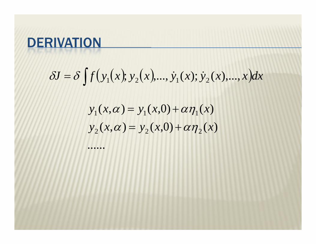
DERIVATIONDERIVATION

( ) ( )( )∫= dxxxyxyxyxyfJ )();(; &&δδ

)()0()( +

( ) ( )( )∫= dxxxyxyxyxyfJ ),...,();(,...,; 2121δδ

)()0,(),()()0,(),(

222

111

xxyxyxxyxy

αηααηα+=+=

......

∫∑ ⎟⎟⎞

⎜⎜⎛ ∂∂

+∂∂

=∂ 2

ii dxdyfdyfdJ ααα&

∫∑ ⎟⎟⎠

⎜⎜⎝ ∂∂

+∂∂

=∂ 1 i ii

dxdy

dy

d αα

αα

αα &

∫ ∫ ⎟⎟⎞

⎜⎜⎛ ∂∂

−∂∂

=∂2 222

dxfdyyfdxyf iiiδ∫ ∫ ⎟⎟

⎠⎜⎜⎝ ∂∂∂∂∂∂1 11

dxydxxy

dxxy iii &&& ααδ

as all curves pass through fixed end point => = 0

∫ ⎟⎟⎠

⎞⎜⎜⎝

⎛∂∂

−∂∂

=2

dxyyf

dxd

yfJ iδδ

&∫ ⎟⎠

⎜⎝ ∂∂1 ydxy ii

⎞⎛ αα

δ dyy ii

0⎟⎠⎞

⎜⎝⎛∂∂

=α 0⎠⎝ ∂

Since y variables are independent then the variation (δy) are independent

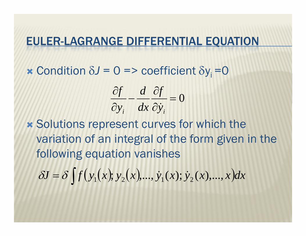
EULER-LAGRANGE DIFFERENTIAL EQUATIONEULER LAGRANGE DIFFERENTIAL EQUATION

Condition δJ = 0 => coefficient δyi =0Condition δJ 0 coefficient δyi 0

0=∂∂

−∂∂ f

ddf

&

Solutions represent curves for which the ∂∂ ii ydxy &

variation of an integral of the form given in the following equation vanishes

( ) ( )( )∫= dxxxyxyxyxyfJ ),...,();(,...,; 2121 &&δδ

HAMILTONIAN >>>> LAGRANGEHAMILTONIAN >>>> LAGRANGE

( )∫∫22

dttqqLLdtI &

With di t t f ti

( )∫∫ ==1

,,1

dttqqLLdtI ii

With coordinate transformationtx →

0=∂∂ fdf

( ) ( )tqqLxyyfqy

iiii

ii

,,,, && →→ 0=

∂−

∂ ii ydxy &

niLdL 3210 ==∂

−∂ ni

qdtq ii

,...,3,2,1,0 ==∂∂ &

Lagrange Equation