wei, d. and rahman, s., "structural reliability analysis by

Probabilistic Engineering Mechanics 22 (2007) 27–38www.elsevier.com/locate/probengmech

Structural reliability analysis by univariate decomposition andnumerical integration

D. Wei, S. Rahman∗

Department of Mechanical and Industrial Engineering, The University of Iowa, Iowa City, IA 52242, United States

Received 22 July 2005; received in revised form 17 April 2006; accepted 1 May 2006Available online 16 June 2006

Abstract

This paper presents a new and alternative univariate method for predicting component reliability of mechanical systems subject to randomloads, material properties, and geometry. The method involves novel function decomposition at a most probable point that facilitates the univariateapproximation of a general multivariate function in the rotated Gaussian space and one-dimensional integrations for calculating the failureprobability. Based on linear and quadratic approximations of the univariate component function in the direction of the most probable point,two mathematical expressions of the failure probability have been derived. In both expressions, the proposed effort in evaluating the failureprobability involves calculating conditional responses at a selected input determined by sample points and Gauss–Hermite integration points.Numerical results indicate that the proposed method provides accurate and computationally efficient estimates of the probability of failure.c© 2006 Elsevier Ltd. All rights reserved.

Keywords: Reliability; Probability of failure; Decomposition methods; Most probable point; Univariate approximation; Numerical integration

1. Introduction

A fundamental problem in time-invariant component relia-bility analysis entails calculation of a multi-fold integral [1–3]

PF ≡ P [g(X) < 0] =

∫g(x)<0

fX(x) dx, (1)

where X = X1, . . . , X N T

∈ RN is a real-valued,N -dimensional (N ≥ 2) random vector defined on aprobability space (Ω ,F, P) comprising the sample space Ω ,the σ -field F , and the probability measure P; g(x) is theperformance function, such that g(x) < 0 represents thefailure domain; PF is the probability of failure; and fX(x)

is the joint probability density function of X, which typicallyrepresents loads, material properties, and geometry. The mostcommon approach to compute the failure probability inEq. (1) involves the first- and second-order reliability methods(FORM/SORM) [1–8], which are respectively based on linear

∗ Corresponding author. Tel.: +1 319 335 5679; fax: +1 319 335 5669.E-mail address: [email protected] (S. Rahman).URL: http://www.engineering.uiowa.edu/∼rahman (S. Rahman).

0266-8920/$ - see front matter c© 2006 Elsevier Ltd. All rights reserved.doi:10.1016/j.probengmech.2006.05.004

(FORM) and quadratic (SORM) approximations of the limit-state surface at a most probable point (MPP) in the standardGaussian space. When the distance βHL between the originand the MPP, a point on the limit-state surface that isclosest to the origin, approaches infinity, FORM/SORM strictlyprovides asymptotic solutions. For non-asymptotic (finiteβHL) applications involving a highly nonlinear performancefunction, its linear or quadratic approximation may not beadequate and therefore resultant FORM/SORM predictionsmust be interpreted with caution [9]. In the latter cases, animportance sampling method developed by Hohenbichler andRackwitz [10] can make the FORM/SORM result arbitrarilyexact, but it may become expensive if a large number ofcostly numerical analyses, such as large-scale finite elementanalysis embedded in the performance function, are involved.Furthermore, the existence of multiple MPPs may lead tolarge errors in standard FORM/SORM approximations [3,8].In that case, multi-point FORM/SORM, along with the systemreliability concept, is required to improve component reliabilityanalysis [8].

Recently, the authors have developed new decompositionmethods, which can solve highly nonlinear reliability problemsmore accurately or more efficiently than FORM/SORM and

http://www.elsevier.com/locate/probengmech

mailto:[email protected]

http://www.engineering.uiowa.edu/~rahman






http://dx.doi.org/10.1016/j.probengmech.2006.05.004

28 D. Wei, S. Rahman / Probabilistic Engineering Mechanics 22 (2007) 27–38

y(v) = y0 +

N∑i=1

yi (vi )︸︷︷︸=y1(v)

+

N∑i1,i2=1i1<i2

yi1i2(vi1 , vi2)

︸︷︷︸=y2(v)

+ · · · +

N∑i1,...,iS=1i1<···<iS

yi1···iS (vi1 , . . . , vis )

︸︷︷︸=yS(v)

+ · · · + y12···N (v1, . . . , vN ),

Box I.

simulation methods [11,12]. A major advantage of thesedecomposition methods, so far based on the mean point [11]or MPP [12] of a random input as reference points,over FORM/SORM is that higher-order approximations ofperformance functions can be achieved using function valuesalone. In particular, an MPP-based univariate method developedin the authors’ previous work involves univariate approximationof the performance function at the MPP, n-point Lagrangeinterpolation in the rotated Gaussian space, and subsequentMonte Carlo simulation [12]. The present work is motivatedby an argument that the MPP-based univariate approximation,if appropriately cast in the rotated Gaussian space, permitsan efficient evaluation of the component failure probability bymultiple one-dimensional integrations.

This paper presents a new and alternative MPP-basedunivariate method for predicting the component reliabilityof mechanical systems subject to random loads, materialproperties, and geometry. Section 2 gives a brief expositionof a novel function decomposition at the MPP thatfacilitates a lower-dimensional approximation of a generalmultivariate function. Section 3 describes the proposedunivariate method, which involves univariate approximationof the performance function at the MPP and univariatenumerical integrations. Section 4 explains the computationaleffort and flowchart of the proposed method. Five numericalexamples involving elementary mathematical functions andstructural/solid-mechanics problems illustrate the methoddeveloped in Section 5. Comparisons have been made withalternative approximate and simulation methods to evaluate theaccuracy and computational efficiency of the new method.

2. Multivariate function decomposition at MPP

Consider a continuous, differentiable, real-valued perfor-mance function g(x) that depends on x = x1, . . . , xN

T∈

RN . If u = u1, . . . , uN T

∈ RN is the standard Gaussianspace, let u∗

=u∗

1, . . . , u∗

N

T denote the MPP or beta point,which is the closest point on the limit-state surface to the ori-gin. The MPP has a distance βHL, which is commonly re-ferred to as the Hasofer–Lind reliability index [1–3], deter-mined by a standard nonlinear constrained optimization. Con-struct an orthogonal matrix R ∈ RN×N whose N th column isα∗

≡ u∗/βHL, i.e., R =[R1 | α∗

], where R1 ∈ RN×N−1 sat-

isfies α∗TR1 = 0 ∈ R1×N−1. The matrix R can be obtained,for example, by Gram–Schmidt orthogonalization. For an or-thogonal transformation u = Rv, let v = v1, . . . , vN

T∈ RN

represent the rotated Gaussian space with the associated MPP

Fig. 1. Performance function approximations by various methods.

v∗=

v∗

1 , . . . , v∗

N−1, v∗

N

T= 0, . . . , 0, βHL

T. The trans-formed limit states h(u) = 0 and y(v) = 0 are therefore themaps of the original limit state g(x) = 0 in the standard Gaus-sian space (u space) and the rotated Gaussian space (v space),respectively. Fig. 1 depicts FORM and SORM approximationsof a limit-state surface at the MPP for N = 2.

Consider a decomposition of a general multivariate functiony(v), which can be viewed as a finite sum [11–13] (see Box I),where y0 is a constant, yi (vi ) is a univariate component functionrepresenting an individual contribution to y(v) by input variablevi acting alone, yi1i2(vi1 , vi2) is a bivariate component functiondescribing the cooperative influence of two input variablesvi1 and vi2 , yi1···iS (vi1 , . . . , viS ) is an S-variate componentfunction quantifying the cooperative effects of S input variablesvi1 , . . . , viS , and so on. If

yS(v) = y0 +

N∑i=1

yi (vi ) +

N∑i1,i2=1i1<i2

yi1i2(vi1 , vi2)

+ · · · +

N∑i1,...,iS=1i1<···<iS

yi1···iS (vi1 , . . . , vis ) (2)

represents a general S-variate approximation of y(v), theunivariate (S = 1) and bivariate (S = 2) approximations

D. Wei, S. Rahman / Probabilistic Engineering Mechanics 22 (2007) 27–38 29

y1(v) and y2(v) respectively provide two- and three-termapproximants of the finite decomposition in the equationgiven in Box I. Similarly, trivariate, quadrivariate, and otherhigher-variate approximations can be derived by appropriatelyselecting the value of S. In the limit when S = N , yS(v)converges to the exact function y(v). In other words, thedecomposition in Eq. (2) generates a convergent sequence ofapproximations of y(v). Readers interested in the fundamentaldevelopment of the decomposition are referred to Xu andRahman [13].

3. New univariate method

3.1. Univariate decomposition of performance function

Consider a univariate approximation of y(v), denoted by

y1(v) ≡ y1(v1, . . . , vN )

=

N∑i=1

y(v∗

1 , . . . , v∗

i−1, vi , v∗

i+1, . . . , v∗

N )

− (N − 1)y(v∗), (3)

where each term in the summation is a function of only onevariable and can subsequently be expanded in a Taylor seriesat the MPP, v∗

=v∗

1 , . . . , v∗

N−1, v∗

N

T= 0, . . . , 0, βHL

T,yielding

y1(v) = y(v∗) +

∞∑j=1

1j !

N∑i=1

∂ j y

∂vji

(v∗)(vi − v∗

i ) j . (4)

In contrast, the Taylor series expansion of y(v) at v∗=

v∗

1 , . . . , v∗

N

T can be expressed by

y(v) = y(v∗)+

∞∑j=1

1j !

N∑i=1

∂ j y

∂vji

(v∗) (

vi − v∗

i

) j+R2 (5)

where the remainder R2 denotes all terms with dimensionstwo and higher. A comparison of Eqs. (4) and (5) indicatesthat the univariate approximation of y1(v) leads to a residualerror y(v) − y1(v) = R2, which includes contributions fromterms of dimension two and higher. For sufficiently smoothy(v) with a convergent Taylor series, the coefficients associatedwith higher-dimensional terms are usually much smaller thanthose with one-dimensional terms. As such, higher-dimensionalterms contribute less to the function, and therefore can beneglected. Nevertheless, Eq. (3) includes all higher-orderunivariate terms, compared with FORM and SORM, whichonly retain linear and quadratic univariate terms, respectively.If the univariate decomposition is not sufficient, bivariate orhigher-variate decompositions may be required [11]. Becauseof the higher cost, these were not included in this study.

In addition to the MPP as the chosen reference point, theaccuracy of the univariate approximation in Eq. (3) may dependon the orientation of the first N − 1 axes. In this work, theorientation is defined by the matrix R. However, an improvedapproximation may be possible by selecting an orientation thatis optimal in some sense. This issue was not considered in thepresent work.

3.2. Univariate integration for failure probability analysis

The proposed univariate approximation of the performancefunction can be rewritten as

y1(v) = yN (vN ) +

N−1∑i=1

yi (vi ) − (N − 1)y(v∗), (6)

where yi (vi ) ≡ y(v∗

1 , . . . , v∗

i−1, vi , v∗

i+1, . . . , v∗

N ); i = 1, N .Due to rotational transformation of the coordinates (see Fig. 1),the univariate component function yN (vN ) in Eq. (6) isexpected to be a linear or a weakly nonlinear function of vN .In fact, yN (vN ) is linear with respect to vN in the classicalFORM/SORM approximation of a performance function in thev space. Nevertheless, if yN (vN ) is invertible, the univariateapproximation y1(v) can be further expressed in a formamenable to an efficient reliability analysis by one-dimensionalnumerical integration. In this work, both linear and quadraticapproximations of yN (vN ) and the resultant equations forfailure probability are derived, as follows.

3.2.1. Linear approximation of yN (vN )

Consider a linear approximation: yN (vN ) = b0 + b1vN ,where coefficients b0 ∈ R and b1 ∈ R (non-zero)are obtained by least-squares approximations from exact or

numerically simulated responses

yN (v(1)N ), . . . , yN (v

(n)N )

at

n sample points along the vN coordinate. The least-squaresapproximation was chosen over interpolation, because theformer minimizes the error when n > 2. Applying thelinear approximation, the component failure probability can beexpressed by

PF ≡ P [y(V) < 0] ∼= P[y1(V) < 0

]∼= P

[b0 + b1VN +

N−1∑i=1

yi (Vi ) − (N − 1)y(v∗) < 0

], (7)

which, on inversion, yields

PF ∼=

P

[VN <

(N − 1)y(v∗) − b0

b1−

1b1

N−1∑i=1

yi (Vi )

],

if b1 > 0

P

[VN ≥

(N − 1)y(v∗) − b0

b1−

1b1

N−1∑i=1

yi (Vi )

],

if b1 < 0.

(8)

Since VN follows standard Gaussian distribution, the failureprobability can also be expressed by

PF ∼= E

[8

((N − 1)y(v∗) − b0

|b1|−

1|b1|

N−1∑i=1

yi (Vi )

)], (9)

where E is the expectation operator and 8 (u) =

(1/

√2π)

∫ u−∞

exp(−ξ2/2

)dξ is the cumulative distribution function of

a standard Gaussian random variable. Note that Eq. (9) provideshigher-order estimates of failure probability if univariatecomponent functions yi (vi ), i = 1, N − 1, are approximated


by terms higher than second order. If yi (vi ), i = 1, N − 1,retain only linear and quadratic terms fitted with appropriatelyselected sample points, Eq. (9) can be further simplified todegenerate to the well-known FORM and SORM (point-fitted)approximations.

3.2.2. Quadratic approximation of yN (vN )

The linear approximation described in the preceding canbe improved by a quadratic approximation: yN (vN ) = b0 +

b1vN + b2v2N , where coefficients b0 ∈ R, b1 ∈ R, and b2 ∈ R

(non-zero) are also obtained by least-squares approximationsfrom exact or numerically simulated responses at n samplepoints along the vN coordinate. Again, the least-squaresapproximation was selected due to error minimization whenn > 3. Similarly, the quadratic approximation of yN (vN )

employed in Eq. (6) leads to

PF ≡ P [y(V) < 0] ∼= P[y1(V) < 0

]∼= P

[b0 + b1VN

+ b2V 2N +

N−1∑i=1

yi (Vi ) − (N − 1)y(v∗) < 0

]. (10)

By defining B(V) ≡ b0 +∑N−1

i=1 yi (Vi ) − (N − 1)y(v∗),where V = V1, . . . , VN−1

T is an N − 1-dimensional standardGaussian vector, the following solutions are derived on the basisof two cases:

(a) Case I — Trivial Solution (b12− 4b2 B < 0; no real roots):

PF ∼=

0, if b2 > 01, if b2 < 0.

(11)

(b) Case II — Non-Trivial Solution (b12

− 4b2 B ≥ 0; two realroots):

PF ∼=

P

−b1 −

√b1

2− 4b2 B(V)

2b2< VN

<−b1 +

√b1

2− 4b2 B(V)

2b2

, if b2 > 0

1 − P

−b1 +

√b1

2− 4b2 B(V)

2b2< VN

<−b1 −

√b1

2− 4b2 B(V)

2b2

, if b2 < 0,

(12)

yielding

PF ∼=1 − b2/ |b2|

2+ E

8

−b1 +

√b1

2− 4b2 B(V)

2b2

− E

8

−b1 −

√b1

2− 4b2 B(V)

2b2

. (13)

Both Eqs. (9) and (13) can be employed for non-trivial solutionsof failure probability. Improvement in the accuracy of results,if any, depends on how strongly yN (vN ) depends on vN .Furthermore, it is possible to develop a generalized version ofEq. (13) when yN (vN ) is highly nonlinear (e.g. polynomial ofan arbitrary order), but invertible. However, due to the rotationaltransformation from the x space to the v space, it is expectedthat the linear approximation of yN (vN ) (Eq. (9)) should resultin a very accurate solution. Hence, the present study is limitedto only linear and quadratic approximations of yN (vN ). It isworth noting that, unlike Eq. (9), Eq. (13) cannot be reduced toFORM/SORM equations, as yN (vN ) includes a second-orderterm.

3.2.3. Univariate integrationThe failure probability expressions in Eqs. (9) and

(13) involve the calculation of the expected values ofseveral multivariate functions of an N − 1-dimensionalstandard Gaussian vector V = V1, . . . , VN−1

T. A genericexpression for such a calculation requires the determination ofE[8( f (V))], where f : RN−1

7→ R is a general mapping of Vand depends on how univariate component functions yi (vi ), i =

1, N −1, are approximated. Unfortunately, the exact probabilitydensity function of f (V) is, in general, not available in closedform. For this reason, it is difficult to calculate E[8( f (V))]

analytically. Numerical integration is not efficient, as 8( f (v))is a multivariate function and becomes impractical when thedimension exceeds three or four.

In reference to Eq. (3), again consider a univariateapproximation of

ln[8 ( f (v))

]∼=

N−1∑i=1

ln [8 ( fi (vi ))]

− (N − 2) ln[8(

f (v∗))]

, (14)

where fi (vi ) ≡ f (v∗

1 , . . . , v∗

i−1, vi , v∗

i+1, . . . , v∗

N−1); i =

1, N − 1 are univariate component functions; and f (v∗) ≡

f (v∗

1 , . . . , v∗

N−1). Hence

8 ( f (v)) = expln[8 ( f (v))

]∼= exp

N−1∑i=1

ln [8 ( fi (vi ))]

− (N − 2) ln[8(

f (v∗))]

=

N−1∏i=1

8 ( fi (vi ))

8 ( f (v∗))N−2 , (15)

yielding

E[8( f (V))] ∼=

N−1∏i=1

E [8 ( fi (Vi ))]

8 ( f (v∗))N−2

=

N−1∏i=1

∫+∞

−∞8( fi (vi ))φ(vi ) dvi

8 ( f (v∗))N−2 , (16)


which involves a product of N −1 univariate integrals with φ(·)

denoting the standard Gaussian probability density function.Using Eq. (16), the nontrivial expressions of failure probabilityin Eqs. (9) and (13) are

PF ∼=

N−1∏i=1

∫+∞

−∞8(

(N−1)y(v∗)−b0−yi (vi )|b1|

)φ(vi ) dvi8

(N−1)y(v∗)−b0−N−1∑i=1

yi (v∗i )

|b1|

N−2 (17)

and

PF ∼=1 − b2/|b2|

2

+

N−1∏i=1

∫+∞

−∞8

(−b1+

√b1

2−4b2 Bi (vi )

2b2

)φ(vi ) dvi[

8

(−b1+

√b1

2−4b2 B(v∗)

2b2

)]N−2

−

N−1∏i=1

∫+∞

−∞8

(−b1−

√b1

2−4b2 Bi (vi )

2b2

)φ(vi ) dvi[

8

(−b1+

√b1

2−4b2 B(v∗)

2b2

)]N−2

(18)

respectively, where Bi (vi ) ≡ B(v∗

1 , . . . , v∗

i−1, vi , v∗

i+1, . . . ,

v∗

N−1). The univariate integration involved in Eqs. (17) or(18) can be evaluated easily by standard one-dimensionalGauss–Hermite numerical quadrature [14]. The decompositionmethod involving univariate approximation (Eq. (3)) andunivariate integration (Eqs. (17) or (18)) is defined as the MPP-based univariate method with numerical integration in thispaper.

4. Computational effort and flow

Consider yi (vi ) ≡ y(v∗

1 , . . . , v∗

i−1, vi , v∗

i+1, . . . , v∗

N ),

i = 1, N − 1, for which n function values yi (v( j)i ) ≡

y(v∗

1 , . . . , v∗

i−1, v( j)i , v∗

i+1, . . . , v∗

N ), j = 1, . . . , n, are required

to be evaluated at integration points vi = v( j)i to perform

an n-order Gauss–Hermite quadrature for the i th integrationin Eqs. (17) or (18). The same procedure is repeated forN − 1 univariate component functions, i.e. for all yi (vi ), i =

1, . . . , N−1. Therefore, the total cost of the proposed univariatemethod, including the n function values of yN (vN ) required forits linear or quadratic approximation, entails a maximum of nNfunction evaluations.1 Note that the above cost is in addition toany function evaluations required for locating the MPP.

Fig. 2 shows the computational flowchart of the MPP-based univariate method with numerical integration. Theimplementation of the method requires the calculation ofyN (vN ) at a user-selected input to obtain coefficients b0, b1,

1 The orders of numerical integration and the number of function values ofyN (vN ) need not be the same. In addition, different orders of integration canbe employed if desired.

and/or b2 and the calculation of yi (vi ), i = 1, . . . , N − 1,at Gauss–Hermite integration points to perform the numericalintegration. Both calculations entail the evaluation of univariatecomponent functions, which are conditional responses. Hence,the proposed effort in determining the failure probability canbe viewed as numerically calculating conditional responsesat a selected input. Compared with the previously developedunivariate method [12], no Monte Carlo simulation is requiredin the present method. The accuracy and efficiency of thenew method depend on both the univariate approximation andnumerical integration. They will be evaluated using severalnumerical examples in a forthcoming section.

In performing n-order Gauss–Hermite quadratures inEqs. (17) or (18), two options for evaluating yi (vi ) areproposed. Option 1 involves calculating yi (v

( j)i ) at integration

points (v∗

1 , . . . , v∗

i−1, v( j)i , v∗

i+1, . . . , v∗

N ), j = 1, n, fromdirect numerical analysis (e.g. finite-element analysis). Whenthe computation of yi (vi ) is expensive, the first option isinefficient if n is required to be large for accurate numericalintegration. The second option involves developing first aunivariate response-surface approximation of yi (vi ) fromselected sample points in the vi -coordinate, followed bynumerical integration of the response-surface approximation.Option 2 is computationally efficient, because no additionalnumerical analysis (e.g. finite-element analysis) is requiredif the order of integration is larger than the number ofsample points. However, an additional layer of response-surfaceapproximation is involved in the second option. Both optionswere explored in numerical examples, as follows.

5. Numerical examples

Five numerical examples involving explicit performancefunctions from mathematical or solid-mechanics problems(Examples 1 and 2) and implicit functions from structural orsolid-mechanics problems (Examples 3, 4, and 5) are presentedto illustrate the MPP-based univariate method with numericalintegration. Whenever possible, comparisons have been madewith the previously developed MPP-based univariate methodwith simulation [12], FORM/SORM, and direct Monte Carlosimulation to evaluate the accuracy and efficiency of the newmethod.

To obtain the linear or quadratic approximation of yN (vN ),n (= 5, 7 or 9) sample points v∗

N − (n − 1)/2, v∗

N −

(n − 3)/2, . . . , v∗

N , . . . , v∗

N + (n − 3)/2, v∗

N + (n − 1)/2were deployed along the vN -coordinate. The same value ofn was employed as the order of Gauss–Hermite quadraturesin Eqs. (17) or (18) of the proposed univariate method withnumerical integration. Furthermore, option 1 was used inExamples 3 and 4 and option 2 was invoked in Examples1, 2 and 5. When using option 2, an nth-order polynomialequation was employed for generating the response-surfaceapproximation of various component functions yi (vi ), i = 1,

N − 1. A 10-order Gauss–Hermite integration was invoked inoption 2. For a consistent comparison, the same value of n wasalso employed as the number of sample points in the previouslydeveloped univariate method with simulation [12]. Hence, the


Fig. 2. Flowchart of the MPP-based univariate method with numerical integration.

total number of function evaluations required by both versionsof the univariate method, in addition to those required forlocating the MPP, is (n −1)N . When comparing computationalefforts by various methods, the number of original performancefunction evaluations is chosen as the primary metric in thispaper.

5.1. Example 1 — Elementary mathematical functions

Consider cubic and quartic performance functions, expres-sed respectively by [12]

g(X1, X2) = 2.2257 −0.025

√2

27(X1 + X2 − 20)3

+33

140(X1 − X2) (19)

g(X1, X2) =52

+1

216(X1 + X2 − 20)4

−33

140(X1 − X2) ,

(20)

where X i , i = 1, 2, are independent, Gaussian randomvariables, each with mean µ = 10 and standard deviationσ = 3. From an MPP search, v∗

= 0, 2.2257T and βHL =

‖v∗‖ = 2.2257 for the cubic function and v∗= 0, 2.5

T andβHL = ‖v∗‖ = 2.5 for the quartic function. For both variants of

the univariate method, a value of n = 5 was selected, resultingin nine function evaluations. Since both performance functionsin the rotated Gaussian space are linear in v2, the proposedmethod involving Eq. (17) was employed to calculate the failureprobability.

Tables 1 and 2 show the results of the failure probabilitycalculated by FORM, SORM [4–6], the MPP-based univariatemethod with simulation [12], the proposed MPP-basedunivariate method with numerical integration, and direct MonteCarlo simulation using 106 samples. The univariate methodwith simulation, which yields exact limit-state equations in thisparticular example, predicts the same probability of failure bythe direct Monte Carlo simulation. The univariate method withnumerical integration also yields exact limit-state equationsand predicts very accurate estimates of failure probabilitywhen compared with simulation results. A slight differencein the failure probability estimates by two versions of theunivariate method is due to the approximations involved inEqs. (7) and (14) of the proposed method. Nevertheless, othercommonly used reliability methods, such as FORM and SORM,underpredict the failure probability by 31% and overpredict thefailure probability by 117% compared with the direct MonteCarlo results. The SORM results are the same as the FORMresults, indicating that there is no improvement over FORM for


Table 1Failure probability for cubic performance function

Method Failure probability Number of function evaluationsa

MPP-based univariate method with numerical integration 0.01895 29b

MPP-based univariate method with simulation [12] 0.01907 29b

FORM 0.01302 21SORM [4–6] 0.01302 204Direct Monte Carlo simulation 0.01907 1000,000

a Total number of times that the original performance function is calculated.b 21 + (n − 1) × N = 21 + (5 − 1) × 2 = 29.

Table 2Failure probability for quartic performance function


MPP-based univariate method with numerical integration 0.003030 29b


FORM 0.006209 21SORM [4–6] 0.006208 212Direct Monte Carlo simulation 0.002886 1000,000


problems involving an inflection point (cubic function) or highnonlinearity (quartic function).

5.2. Example 2 — Burst margin of a rotating disk

Consider an annular disk of inner radius Ri , outer radiusRo, and constant thickness t Ro (plane stress), as shownin Fig. 3. The disk is subject to an angular velocity, ω,about an axis perpendicular to its plane at the centre. Themaximum allowable angular velocity, ωa , when tangentialstresses through the thickness reach the material’s ultimatestrength, Su , factored by a material utilization factor αm , is [15]

ωa =

[3αm Su (Ro − Ri )

ρ(R3

o − R3i

) ]1/2

, (21)

where ρ is the mass density of the material. According to anSAE G-11 standard, the satisfactory performance of the disk isdefined when the burst margin Mb, defined as

Mb ≡ωa

ω=

[3αm Su (Ro − Ri )

ρω2(R3

o − R3i

) ]1/2

, (22)

exceeds 0.374 73 [16]. If random variables X1 = αm , X2 =

Su , X3 = ω, X4 = ρ, X5 = Ro, and X6 = Ri havetheir statistical properties defined in Table 3, the performancefunction becomes

g(X) = Mb(X1, X2, X3, X4, X5, X6) − 0.374 73. (23)

Table 4 presents the predicted failure probability of the diskand the associated computational effort using new and ex-isting MPP-based univariate methods, FORM, Hohenbichler’sSORM [5], and direct Monte Carlo simulation (106 samples).For univariate methods, a value of n = 7 was selected. For the

Fig. 3. Rotating annular disk subject to angular velocity.

univariate method with numerical integration, the failure prob-abilities based on linear (Eq. (17)) and quadratic (Eq. (18)) ap-proximations are almost identical, which verifies the adequacyof the linear approximation of yN (vN ) in this example. Theresults also indicate that the univariate methods using eithersimulation or numerical integration produce the most accuratesolution. FORM and SORM slightly underpredict the failureprobability. Both univariate methods surpass the efficiency ofSORM in solving this particular reliability problem.

5.3. Example 3 — Ten-bar truss structure

A ten-bar, linear-elastic, truss structure, shown in Fig. 4,was studied in this example to examine the accuracy andefficiency of the proposed reliability method. The Young’s


Table 3Statistical properties of random input for rotating disk

Random variable Mean Standard deviation Probability distribution

αm 0.9377 0.0459 Weibulla

Su , ksi 220 5 Gaussianω, rpm 24 0.5 Gaussianρ, lb − s2/in.4 0.29/gb 0.0058/gb Uniformc

Ro, in. 24 0.5 GaussianRi , in. 8 0.3 Gaussian

a Scale parameter = 25.508; shape parameter = 0.958.b g = 385.82 in./s2.c Uniformly distributed over (0.28, 0.3).

Table 4Failure probability of rotating disk


MPP-based univariate method with numerical integrationLinear (Eq. (17)) 0.00099 167b

Quadratic (Eq. (18)) 0.00099 167b


FORM 0.00089 131SORM (Hohenbichler) [5] 0.00097 378Direct Monte Carlo simulation 0.00104 1000,000


Fig. 4. A ten-bar truss structure.

modulus of the material is 107 psi. Two concentrated forces of105 lb are applied at nodes 2 and 3, as shown in Fig. 4. Thecross-sectional area X i , i = 1, . . . , 10 for each bar followsa truncated normal distribution clipped at xi = 0 and hasmean µ = 2.5 in.2 and standard deviation σ = 0.5 in.2.According to the loading condition, the maximum displacement[v3(X1, . . . , X10)] occurs at node 3, where the permissibledisplacement is limited to 18 in., leading to g(X) = 18 −

v3 (X1, . . . , X10).From an MPP search involving finite-difference gradients,

βHL = ‖v∗‖ = 1.3642. Table 5 shows the failureprobability of the truss, calculated using the proposed MPP-based univariate method with numerical integration, MPP-based univariate method with simulation [12], FORM, threevariants of SORM due to Breitung [4], Hohenbichler [5] and

Cai and Elishakoff [6], and direct Monte Carlo simulation(106 samples). For univariate methods, a value of n = 7was selected. From Table 5, both versions of the univariatemethod predict the failure probability more accurately thanFORM and all three variants of SORM. This is becauseunivariate methods are able to approximate the performancefunction more accurately than FORM/SORM. The univariatemethod with numerical integration involving the quadraticapproximation of yN (vN ) yields a slightly more accurate resultthan that based on its linear approximation. A comparison of thenumber of function evaluations, also listed in Table 5, indicatesthat the computational effort by the MPP-based univariatemethods is slightly larger than FORM, but much less thanSORM.

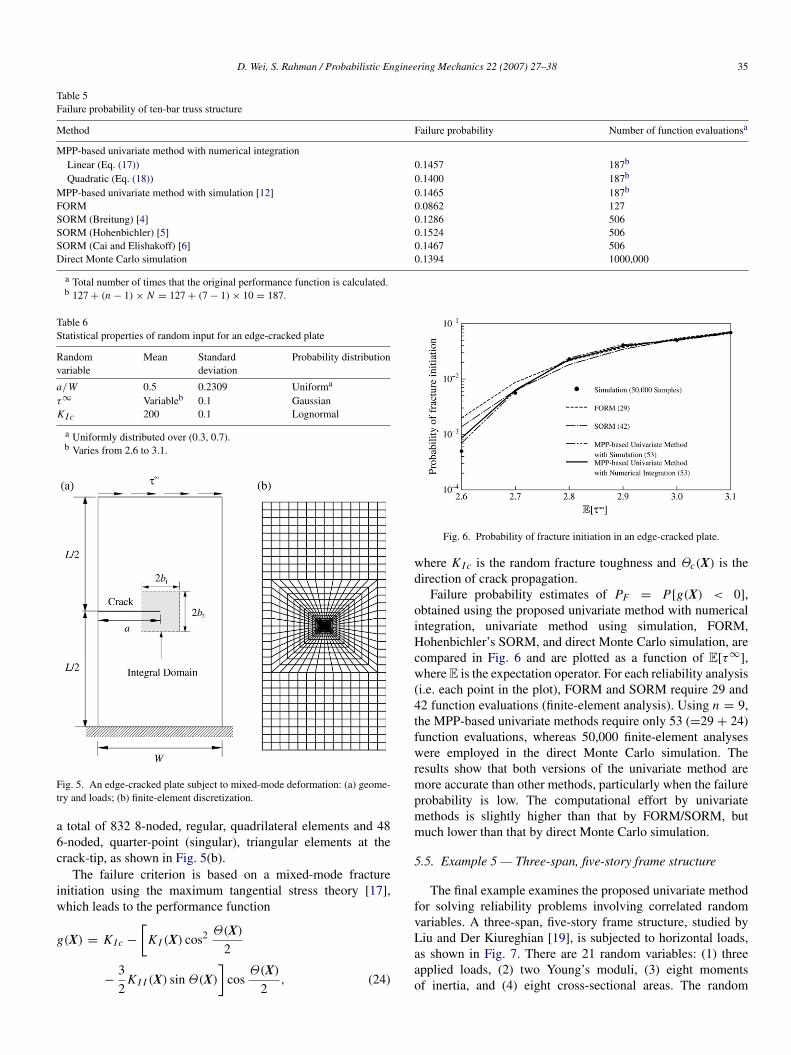
5.4. Example 4 — Mixed-mode fracture-mechanics analysis

The fourth example involves an isotropic, homogeneous,edge-cracked plate, presented to illustrate mixed-mode proba-bilistic fracture-mechanics analysis using the proposed univari-ate method. As shown in Fig. 5(a), a plate of length L = 16units and width W = 7 units is fixed at the bottom and sub-jected to a far-field and a shear stress τ∞ applied at the top.The elastic modulus and Poisson’s ratio are 1 unit and 0.25,respectively. A plane strain condition was assumed. The statis-tical property of the random input X = a/W, τ∞, K I c

T isdefined in Table 6.

Due to the far-field shear stress τ∞, the plate is subjectedto mixed-mode deformation involving fracture modes I andII [17]. The mixed-mode stress-intensity factors K I (X) andK I I (X) were calculated using an interaction integral [18]. Theplate was analysed using the finite-element method, involving


Table 5Failure probability of ten-bar truss structure


MPP-based univariate method with numerical integrationLinear (Eq. (17)) 0.1457 187b

Quadratic (Eq. (18)) 0.1400 187b


FORM 0.0862 127SORM (Breitung) [4] 0.1286 506SORM (Hohenbichler) [5] 0.1524 506SORM (Cai and Elishakoff) [6] 0.1467 506Direct Monte Carlo simulation 0.1394 1000,000


Table 6Statistical properties of random input for an edge-cracked plate

Randomvariable

Mean Standarddeviation

Probability distribution

a/W 0.5 0.2309 Uniforma

τ∞ Variableb 0.1 GaussianK I c 200 0.1 Lognormal

a Uniformly distributed over (0.3, 0.7).b Varies from 2.6 to 3.1.

Fig. 5. An edge-cracked plate subject to mixed-mode deformation: (a) geome-try and loads; (b) finite-element discretization.

a total of 832 8-noded, regular, quadrilateral elements and 486-noded, quarter-point (singular), triangular elements at thecrack-tip, as shown in Fig. 5(b).

The failure criterion is based on a mixed-mode fractureinitiation using the maximum tangential stress theory [17],which leads to the performance function

g(X) = K I c −

[K I (X) cos2 Θ(X)

2

−32

K I I (X) sin Θ(X)

]cos

Θ(X)

2, (24)

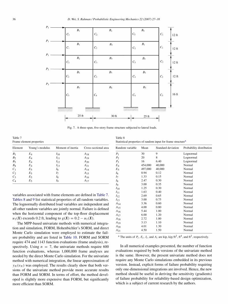
Fig. 6. Probability of fracture initiation in an edge-cracked plate.

where K I c is the random fracture toughness and Θc(X) is thedirection of crack propagation.

Failure probability estimates of PF = P[g(X) < 0],obtained using the proposed univariate method with numericalintegration, univariate method using simulation, FORM,Hohenbichler’s SORM, and direct Monte Carlo simulation, arecompared in Fig. 6 and are plotted as a function of E[τ∞

],where E is the expectation operator. For each reliability analysis(i.e. each point in the plot), FORM and SORM require 29 and42 function evaluations (finite-element analysis). Using n = 9,the MPP-based univariate methods require only 53 (=29 + 24)function evaluations, whereas 50,000 finite-element analyseswere employed in the direct Monte Carlo simulation. Theresults show that both versions of the univariate method aremore accurate than other methods, particularly when the failureprobability is low. The computational effort by univariatemethods is slightly higher than that by FORM/SORM, butmuch lower than that by direct Monte Carlo simulation.

5.5. Example 5 — Three-span, five-story frame structure

The final example examines the proposed univariate methodfor solving reliability problems involving correlated randomvariables. A three-span, five-story frame structure, studied byLiu and Der Kiureghian [19], is subjected to horizontal loads,as shown in Fig. 7. There are 21 random variables: (1) threeapplied loads, (2) two Young’s moduli, (3) eight momentsof inertia, and (4) eight cross-sectional areas. The random


Fig. 7. A three-span, five-story frame structure subjected to lateral loads.

Table 7Frame element properties

Element Young’s modulus Moment of inertia Cross-sectional area

B1 E4 I10 A18B2 E4 I11 A19B3 E4 I12 A20B4 E4 I13 A21C1 E5 I6 A14C2 E5 I7 A15C3 E5 I8 A16C4 E5 I9 A17

variables associated with frame elements are defined in Table 7.Tables 8 and 9 list statistical properties of all random variables.The lognormally distributed load variables are independent andall other random variables are jointly normal. Failure is definedwhen the horizontal component of the top-floor displacementu1(X) exceeds 0.2 ft, leading to g(X) = 0.2 − u1(X).

The MPP-based univariate methods with numerical integra-tion and simulation, FORM, Hohenbichler’s SORM, and directMonte Carlo simulation were employed to estimate the fail-ure probability and are listed in Table 10. FORM and SORMrequire 474 and 1143 function evaluations (frame analysis), re-spectively. Using n = 7, the univariate methods require 600function evaluations, whereas 1,000,000 frame analyses areneeded by the direct Monte Carlo simulation. For the univariatemethod with numerical integration, the linear approximation ofyN (vN ) was employed. The results clearly show that both ver-sions of the univariate method provide more accurate resultsthan FORM and SORM. In terms of effort, the method devel-oped is slightly more expensive than FORM, but significantlymore efficient than SORM.

Table 8Statistical properties of random input for frame structurea

Random variable Mean Standard deviation Probability distribution

P1 30 9 LognormalP2 20 8 LognormalP3 16 6.40 LognormalE4 454,000 40,000 NormalE5 497,000 40,000 NormalI6 0.94 0.12 NormalI7 1.33 0.15 NormalI8 2.47 0.30 NormalI9 3.00 0.35 NormalI10 1.25 0.30 NormalI11 1.63 0.40 NormalI12 2.69 0.65 NormalI13 3.00 0.75 NormalA14 3.36 0.60 NormalA15 4.00 0.80 NormalA16 5.44 1.00 NormalA17 6.00 1.20 NormalA18 2.72 1.00 NormalA19 3.13 1.10 NormalA20 4.01 1.30 NormalA21 4.50 1.50 Normal

a The units of Pi , Ei , Ii , and Ai are kip, kip/ft2, ft4, and ft2, respectively.

In all numerical examples presented, the number of functionevaluations required by both versions of the univariate methodis the same. However, the present univariate method does notrequire any Monte Carlo simulations embedded in its previousversion. Instead, explicit forms of failure probability requiringonly one-dimensional integrations are involved. Hence, the newmethod should be useful in deriving the sensitivity (gradients)of failure probability for reliability-based design optimization,which is a subject of current research by the authors.


Table 9Correlation coefficients of random input for frame structure

P1 P2 P3 E4 E5 I6 I7 I8 I9 I10 I11 I12 I13 A14 A15 A16 A17 A18 A19 A20 A21

P1 1.0P2 0. 1.0P3 0. 0. 1.0E4 0. 0. 0. 1.0E5 0. 0. 0. 0.9 1.0I6 0. 0. 0. 0. 0. 1.0I7 0. 0. 0. 0. 0. 0.13 1.0I8 0. 0. 0. 0. 0. 0.13 0.13 1.0I9 0. 0. 0. 0. 0. 0.13 0.13 0.13 1.0I10 0. 0. 0. 0. 0. 0.13 0.13 0.13 0.13 1.0I11 0. 0. 0. 0. 0. 0.13 0.13 0.13 0.13 0.13 1.0I12 0. 0. 0. 0. 0. 0.13 0.13 0.13 0.13 0.13 0.13 1.0I13 0. 0. 0. 0. 0. 0.13 0.13 0.13 0.13 0.13 0.13 0.13 1.0A14 0. 0. 0. 0. 0. 0.95 0.13 0.13 0.13 0.13 0.13 0.13 0.13 1.0A15 0. 0. 0. 0. 0. 0.13 0.95 0.13 0.13 0.13 0.13 0.13 0.13 0.13 1.0A16 0. 0. 0. 0. 0. 0.13 0.13 0.95 0.13 0.13 0.13 0.13 0.13 0.13 0.13 1.0A17 0. 0. 0. 0. 0. 0.13 0.13 0.13 0.95 0.13 0.13 0.13 0.13 0.13 0.13 0.13 1.0A18 0. 0. 0. 0. 0. 0.13 0.13 0.13 0.13 0.95 0.13 0.13 0.13 0.13 0.13 0.13 0.13 1.0A19 0. 0. 0. 0. 0. 0.13 0.13 0.13 0.13 0.13 0.95 0.13 0.13 0.13 0.13 0.13 0.13 0.13 1.0A20 0. 0. 0. 0. 0. 0.13 0.13 0.13 0.13 0.13 0.13 0.95 0.13 0.13 0.13 0.13 0.13 0.13 0.13 1.0A21 0. 0. 0. 0. 0. 0.13 0.13 0.13 0.13 0.13 0.13 0.13 0.95 0.13 0.13 0.13 0.13 0.13 0.13 0.13 1.0

Table 10Failure probability of frame structure


MPP-based univariate method with numerical integration 3.829 × 10−4 600b

MPP-based univariate method with simulation [12] 3.720 × 10−4 600b

FORM 7.891 × 10−4 474SORM (Hohenbichler) [5] 1.402 × 10−4 1143Direct Monte Carlo simulation 3.630 × 10−4 1000,000


6. Conclusions

A new univariate method was developed for predictingthe component reliability of mechanical systems subjectto random loads, material properties, and geometry. Themethod involves novel function decomposition at the mostprobable point, which facilitates univariate approximation ofa general multivariate function in the rotated Gaussian spaceand one-dimensional integrations for calculating the failureprobability. Based on linear and quadratic approximations ofthe univariate component function in the direction of the mostprobable point, two mathematical expressions of the failureprobability were derived. In both expressions, the proposedeffort in evaluating the failure probability involves calculatingconditional responses at a selected input determined by samplepoints and Gauss–Hermite integration points. The results offive numerical examples involving elementary mathematicalfunctions and structural/solid-mechanics problems indicate thatthe proposed method provides accurate and computationallyefficient estimates of the probability of failure. Compared withthe authors’ previous work, no Monte Carlo simulation isrequired in the present version of the univariate method thathas been developed. Although both versions of the univariate

method have comparable computational efficiencies, the newmethod should be useful in deriving the sensitivity of the failureprobability for reliability-based design optimization, which isthe ultimate goal of probabilistic mechanics.

Acknowledgment

The authors would like to acknowledge the financial supportof the US National Science Foundation under Grant No. DMI-0355487.

References

[1] Madsen HO, Krenk S, Lind NC. Methods of structural safety. EnglewoodCliffs (NJ): Prentice-Hall, Inc.; 1986.

[2] Rackwitz R. Reliability analysis — A review and some perspectives.Structural Safety 2001;23(4):365–95.

[3] Ditlevsen O, Madsen HO. Structural reliability methods. Chichester: JohnWiley & Sons Ltd.; 1996.

[4] Breitung K. Asymptotic approximations for multinormal integrals. ASCEJournal of Engineering Mechanics 1984;110(3):357–66.

[5] Hohenbichler M, Gollwitzer S, Kruse W, Rackwitz R. New light on first-and second-order reliability methods. Structural Safety 1987;4:267–84.


[6] Cai GQ, Elishakoff I. Refined second-order reliability analysis. StructuralSafety 1994;14:267–76.

[7] Tvedt L. Distribution of quadratic forms in normal space — Applicationto structural reliability. ASCE Journal of Engineering Mechanics 1990;116(6):1183–97.

[8] Der Kiureghian A, Dakessian T. Multiple design points in first andsecond-order reliability. Structural Safety 1998;20(1):37–49.

[9] Nie J, Ellingwood BR. Directional methods for structural reliabilityanalysis. Structural Safety 2000;22:233–49.

[10] Hohenbichler M, Rackwitz R. Improvement of second-order reliabilityestimates by importance sampling. ASCE Journal of EngineeringMechanics 1988;114(12):2195–8.

[11] Xu H, Rahman S. Decomposition methods for structural reliabilityanalysis. Probabilistic Engineering Mechanics 2005;20:239–50.

[12] Rahman S, Wei D. A univariate approximation at most probable pointfor higher-order reliability analysis. International Journal of Solids andStructures 2006;43:2820–39.

[13] Xu H, Rahman S. A generalized dimension-reduction method for multi-dimensional integration in stochastic mechanics. International Journal forNumerical Methods in Engineering 2004;61:1992–2019.

[14] Abramowitz M, Stegun I. Handbook of mathematical functions. 9th ed.New York (NY): Dover Publications, Inc.; 1972.

[15] Boresi AP, Schmidt RJ. Advanced mechanics of materials. 6th ed. NewYork (NY): John Wiley & Sons, Inc.; 2003.

[16] Penmetsa R, Grandhi R. Adaptation of fast Fourier transformations toestimate structural failure probability. Finite Elements in Analysis andDesign 2003;39:473–85.

[17] Anderson TL. Fracture mechanics: Fundamentals and applications. 2nded. Boca Raton (FL): CRC Press Inc.; 1995.

[18] Yau JF, Wang SS, Corten HT. A mixed-mode crack analysis of isotropicsolids using conservation laws of elasticity. Journal of Applied Mechanics1980;47:335–41.

[19] Liu PL, Der Kiureghian A. Optimization algorithms for structuralreliability analysis. Report no. UCB/SESM-86/09. Berkeley (CA); 1986.

wei, d. and rahman, s., "structural reliability analysis by

Documents