weibull analysis and area scaling for infrared window ... · nawcwd tp 8806 . weibull analysis and...
TRANSCRIPT
NAWCWD TP 8806
Weibull Analysis and Area Scaling
for Infrared Window Materials
by
Daniel C. Harris
Research Division
Research and Engineering Group
AUGUST 2016
NAVAL AIR WARFARE CENTER WEAPONS DIVISION CHINA LAKE, CA 93555-6100
DISTRIBUTION STATEMENT A. Approved for
public release; distribution is unlimited.
Naval Air Warfare Center Weapons Division
FOREWORD
This report provides a tutorial on the Weibull distribution of strength of ceramic
materials and the use of the maximum likelihood method of American Society for
Testing and Materials (ASTM) C1239 to obtain Weibull parameters from a set of test
coupons. Parameters compiled from test data of infrared window materials are used to
predict the static probability of failure of an optical window in the absence of slow crack
growth. This report emphasizes how the strength of a window scales inversely with the
size of the window.
This report was reviewed for technical accuracy by Howard Poisl, Thomas M.
Hartnett, and Lee M. Goldman.
Approved by Under authority of
A. VAN NEVEL, Head B. K. COREY
Research Division RDML, U.S. Navy
4 August 2016 Commander
Released for publication by
J. L. JOHNSON
Director for Research and Engineering
NAWCWD Technical Publication 8806
Published by ..................................................................... Technical Communication Office
Collation ...................................................................................................... Cover, 19 leaves
First printing ............................................................................... 8 paper, 4 electronic media

REPORT DOCUMENTATION PAGE Form Approved
OMB No. 0704-0188 The public reporting burden for this collection of information is estimated to average 1 hour per response, including the time for reviewing instructions, searching existing data sources, gathering and maintaining the data needed, and completing and reviewing the collection of information. Send comments regarding this burden estimate or any other aspect of this collection of information, including suggestions for reducing the burden, to the Department of Defense, Executive Service Directorate (0704-0188). Respondents should be aware that notwithstanding any other provision of law, no person shall be subject to any penalty for failing to comply with a collection of information if it does not display a currently valid OMB control number. PLEASE DO NOT RETURN YOUR FORM TO THE ABOVE ORGANIZATION.
1. REPORT DATE (DD-MM-YYYY)
04-08-2016
2. REPORT TYPE
Final
3. DATES COVERED (From - To)
1 October 2015–6 July 2016
4. TITLE AND SUBTITLE
Weibull Analysis and Area Scaling for Infrared Window Materials (U)
5a. CONTRACT NUMBER
N/A
5b. GRANT NUMBER
N/A
5c. PROGRAM ELEMENT NUMBER
N/A
6. AUTHOR(S)
Daniel C. Harris
5d. PROJECT NUMBER
N/A
5e. TASK NUMBER
N/A
5f. WORK UNIT NUMBER
N/A
7. PERFORMING ORGANIZATION NAME(S) AND ADDRESS(ES)
Naval Air Warfare Center Weapons Division
1 Administration Circle
China Lake, California 93555-6100
8. PERFORMING ORGANIZATION REPORT NUMBER
NAWCWD TP 8806
9. SPONSORING/MONITORING AGENCY NAME(S) AND ADDRESS(ES)
Office of Naval Research
875 North Randolph Street
Arlington, Virginia 22203
10. SPONSOR/MONITOR’S ACRONYM(S)
ONR
11. SPONSOR/MONITOR’S REPORT NUMBER(S)
N/A
12. DISTRIBUTION/AVAILABILITY STATEMENT
DISTRIBUTION STATEMENT A. Approved for public release.
13. SUPPLEMENTARY NOTES
None.
14. ABSTRACT
(U) This report provides a tutorial on the Weibull distribution of strength of ceramic materials and the use of the maximum
likelihood method of American Society for Testing and Materials (ASTM) C1239 to obtain Weibull parameters from a set of test
coupons. Parameters compiled from test data of infrared window materials are used to predict the static probability of failure of an
optical window in the absence of slow crack growth. This report emphasizes how the strength of a window scales inversely with the
size of the window. Test data are given for aluminum oxynitride (ALON), calcium fluoride, chemical vapor deposited (CVD) diamond,
fused quartz, germanium, magnesium fluoride, yttria-magnesia nanocomposite optical ceramic (NCOC), polycrystalline alumina,
sapphire (a-plane, c-plane, and r-plane), magnesium aluminum spinel, yttria, zinc selenide, and zinc sulfide (standard and multispectral
grades).
15. SUBJECT TERMS
ALON, Aluminum Oxynitride, Area Scaling of Strength, ASTM C1239, Calcium Fluoride, Ceramic Mechanical Strength, CVD Diamond,
Fused Quartz, Germanium, Magnesium Fluoride, Maximum Likelihood Method, NCOC, Polycrystalline Alumina, Sapphire, Spinel, Static
Probability of Failure, Weibull Analysis, Yttria, Yttria-Magnesia Nanocomposite Optical Ceramic, Zinc Selenide, Zinc Sulfide
16. SECURITY CLASSIFICATION OF: 17. LIMITATION OF ABSTRACT
SAR
18. NUMBER OF PAGES
36
19a. NAME OF RESPONSIBLE PERSON
Daniel C. Harris a. REPORT
UNCLASSIFIED b. ABSTRACT
UNCLASSIFIED c. THIS PAGE
UNCLASSIFIED 19b. TELEPHONE NUMBER (include area code)
(760) 939-1649
Standard Form 298 (Rev. 8-98) Prescribed by ANSI Std. Z39.18

UNCLASSIFIED
SECURITY CLASSIFICATION OF THIS PAGE (When Data Entered)
Standard Form 298 Back SECURITY CLASSIFICATION OF THIS PAGE UNCLASSIFIED

NAWCWD TP 8806
1
CONTENTS
Executive Summary ............................................................................................................ 3
Introduction ......................................................................................................................... 5
Weibull Equation in American Society for Testing and Materials (ASTM) C1239 .......... 5
Effective Area Ae ................................................................................................................ 7
Ring-on-Ring Geometry .............................................................................................. 7
Pressure-on-Ring Geometry ........................................................................................ 9
Weibull Analysis in ASTM C1239 ................................................................................... 10
Weibull Scale Parameter σo .............................................................................................. 13
Strength Scales With Area Under Stress .......................................................................... 15
Experimental Confirmation of Weibull Area Scaling ...................................................... 15
Compilation of Weibull Parameters for Infrared Window Materials ............................... 17
Weibull Probability of Survival Without Slow Crack Growth ......................................... 22
General Approach to Weibull Probability of Survival ..................................................... 24
Some Caveats for Window Design ............................................................................ 27
Maximum Likelihood Method .......................................................................................... 28
Summary ........................................................................................................................... 30
References ......................................................................................................................... 32

NAWCWD TP 8806
2
Figures:
1. Weibull Curve (Cumulative Probability of Failure) Fit to
Observed Strengths (Failure Stress) of 10 Test Coupons .................................. 5
2. Geometry of Ring-on-Ring Flexure Test of a Polished Ceramic Disk .............. 7
3. Side View of Circular Sensor Window Subjected to a Uniform Pressure
Difference Between the Two Faces ................................................................... 9
4. Initial Excel Spreadsheet With a Guess m = 6 for the Weibull
Modulus in Cell B17 ........................................................................................ 10
5. Excel Spreadsheet After Solver Has Found m = 10.28 for the
Weibull Modulus in Cell B17 to Make the Sum in Cell D22 Zero ................. 12
6. Demonstration of Weibull Area Scaling for Sintered Silicon
Carbide 3- and 4-Point Flexure Bars ............................................................... 16
7. Window in a Frame With Pressure Difference P = 0.5 MPa Across the
Window ............................................................................................................ 22
8. Weibull Plot of Strengths of 25 Transparent Polycrystalline Alumina
Disks With Radius 1.90 cm and Thickness 0.203 cm Using a
Ring-on-Ring Test Fixture With Load Radius 0.794 cm and
Support Radius 1.588 cm Tested in Air at 20% Relative
Humidity at 21°C With Crosshead Speed 0.508 mm/min ............................... 23
9. Computing Weibull Probability of Survival by Dividing
a Window Into Many Surface Elements and Computing
the Probability of Survival of Each Element ................................................... 25
10. Weibull Cumulative Probability of Failure Pf From Equation 1 and
Probability Density From Equation 20 for m = 6.48 and σθ = 555.8 MPa ...... 28
Tables:
1. Unbiasing Factor for Weibull Modulus From ASTM C1239 .......................... 13
2. Strengths of Infrared Window Materials: ASTM C1239
Weibull Parameters .......................................................................................... 18
3. Weibull Probability of Survival of a Window Found From
the Stress in Each Element of Area ................................................................. 26
NAWCWD TP 8806
3
EXECUTIVE SUMMARY
A tutorial is provided on the Weibull distribution of strength of ceramic materials
and use of the maximum likelihood method of American Society for Testing and
Materials (ASTM) C1239 to obtain Weibull parameters from test data. Parameters are
compiled from testing of the infrared window materials aluminum oxynitride (ALON),
calcium fluoride, chemical vapor deposited (CVD) diamond, fused quartz, germanium,
magnesium fluoride, yttria-magnesia nanocomposite optical ceramic (NCOC),
polycrystalline alumina, sapphire (a-plane, c-plane, and r-plane), magnesium aluminum
spinel, yttria, zinc selenide, and zinc sulfide (standard and multispectral grades). Weibull
parameters are used to predict the static probability of failure of an optical window in the
absence of slow crack growth. This report illustrates how the strength of a window scales
inversely with the size of the window.
NAWCWD TP 8806
4
This page intentionally left blank.
NAWCWD TP 8806
5
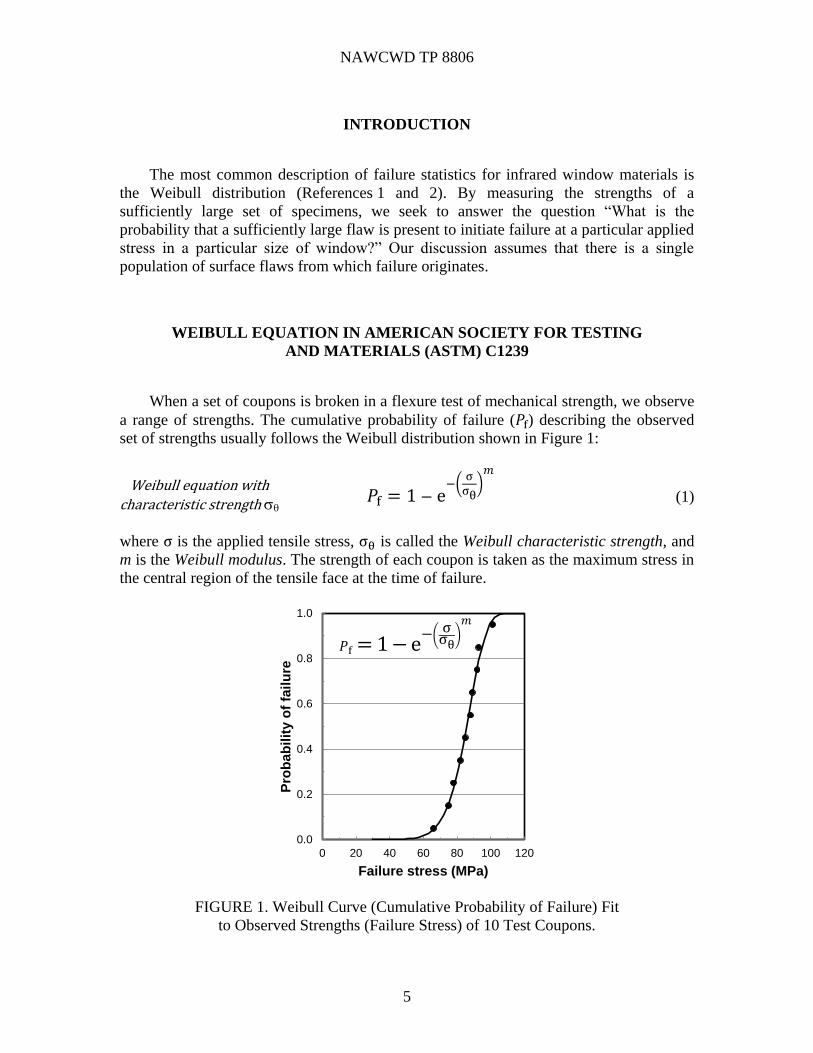
INTRODUCTION
The most common description of failure statistics for infrared window materials is
the Weibull distribution (References 1 and 2). By measuring the strengths of a
sufficiently large set of specimens, we seek to answer the question “What is the
probability that a sufficiently large flaw is present to initiate failure at a particular applied
stress in a particular size of window?” Our discussion assumes that there is a single
population of surface flaws from which failure originates.
WEIBULL EQUATION IN AMERICAN SOCIETY FOR TESTING
AND MATERIALS (ASTM) C1239
When a set of coupons is broken in a flexure test of mechanical strength, we observe
a range of strengths. The cumulative probability of failure (𝑃f) describing the observed
set of strengths usually follows the Weibull distribution shown in Figure 1:
Weibull equation with
characteristic strength 𝑃f = 1 − e
−(σ
σθ)
𝑚
(1)
where σ is the applied tensile stress, σθ is called the Weibull characteristic strength, and
m is the Weibull modulus. The strength of each coupon is taken as the maximum stress in
the central region of the tensile face at the time of failure.
FIGURE 1. Weibull Curve (Cumulative Probability of Failure) Fit
to Observed Strengths (Failure Stress) of 10 Test Coupons.
0.0
0.2
0.4
0.6
0.8
1.0
0 20 40 60 80 100 120
Pro
ba
bil
ity o
f fa
ilu
re
Failure stress (MPa)
Cleartranoptimum m
fit
𝑃f = 1 − e−(
σσθ
)
𝑚

NAWCWD TP 8806
6
The cumulative probability of failure 𝑃f ranges from 0 at low stress to 1 at
sufficiently high stress in Figure 1. The spread of strengths is related to the Weibull
modulus, m, which is typically in the range 3 to 15 for polished optical ceramics. The
larger the value of m, the narrower is the distribution of strength. A narrow distribution of
strengths (a large Weibull modulus) is desirable for a reliable mechanical design. The
greater the characteristic strength, σθ, the greater is the mean strength of the set
of coupons.
Weibull characteristic strength σθ in Equation 1 is not a material property. It
depends on specimen size, the type of mechanical test, and the dimensions of the test
fixture. If specimens fail from surface flaws, the effective area under tension (𝐴e) can be
incorporated into the Weibull equation. In a given mechanical test at a particular stress,
a specimen of effective area 𝐴𝑒 has the same probability of failure as a sample with
geometric area 𝐴𝑒 loaded in uniform uniaxial tension. Effective area accounts for the
kind of test being done and for specimen size and test fixture dimensions:
𝑊𝑒𝑖𝑏𝑢𝑙𝑙 𝑒𝑞𝑢𝑎𝑡𝑖𝑜𝑛 𝑤𝑖𝑡ℎ𝑊𝑒𝑖𝑏𝑢𝑙𝑙 𝑠𝑐𝑎𝑙𝑒 𝑓𝑎𝑐𝑡𝑜𝑟 σo
𝑃f = 1 − e−(
𝐴e𝐴o
)(σ
σo)
𝑚
(2)
Equation 2 incorporates effective area 𝐴e and contains the Weibull scale factor σo in
place of the characteristic strength σθ. The scale factor σo is ideally a property of the
material and the way it is fabricated. In the exponent of Equation 2, 𝐴o is taken as one
unit of area, such as 1 cm2, to cancel the units of 𝐴e, because an exponent must be
dimensionless. Equating exponents in Equations 1 and 2 provides the relationship
between the material property σo and the curve-fitting parameter σθ from Figure 1:
− (σ
σθ)
𝑚= − (
𝐴e
𝐴o) (
σ
σo)
𝑚 σo = σθ (
𝐴e
𝐴o)
1/𝑚 (3)
The symbol “” is read “implies that”. The Weibull scale factor σo is the Weibull
characteristic strength when the effective area of the specimen is 1 cm2.
The expected mean strength of replicate samples with effective area 𝐴e is
Expected mean strength = σo (𝐴o
𝐴e)
1/𝑚Γ (1 +
1
𝑚) (4)
Eq. (1) Eq. (2)
NAWCWD TP 8806
7
where Γ is the gamma function of the argument (1 + 1 𝑚⁄ ). You can compute the
numerical value of Γ in an Excel® spreadsheet with the statement
“=exp(gammaln(1+1/m))”.*
𝛔𝛉: Weibull characteristic strength obtained by fitting strengths of test specimens
to Equation 1.
𝛔𝐨: Weibull scale factor computed from σθ with Equation 3. σo would be the
characteristic strength if test samples had an effective area of 𝐴e = 1 cm2.
Caveat Emptor. There is inconsistent use of the symbols σθ and σo and the terms
“characteristic strength” and “scale factor” in the literature. It is impeccable practice to
write the Weibull equation that you are using and to write the names of the different
symbols.
EFFECTIVE AREA Ae
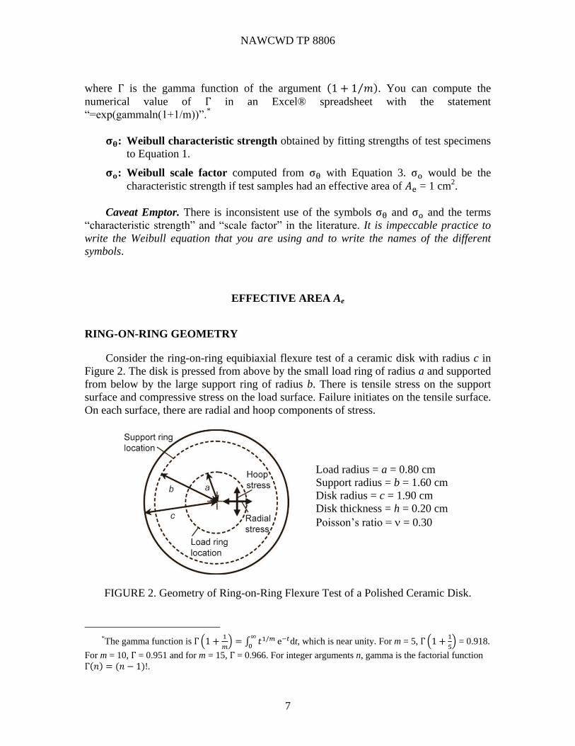
RING-ON-RING GEOMETRY
Consider the ring-on-ring equibiaxial flexure test of a ceramic disk with radius c in
Figure 2. The disk is pressed from above by the small load ring of radius a and supported
from below by the large support ring of radius b. There is tensile stress on the support
surface and compressive stress on the load surface. Failure initiates on the tensile surface.
On each surface, there are radial and hoop components of stress.
Load radius = a = 0.80 cm
Support radius = b = 1.60 cm
Disk radius = c = 1.90 cm
Disk thickness = h = 0.20 cm
Poisson’s ratio = = 0.30
FIGURE 2. Geometry of Ring-on-Ring Flexure Test of a Polished Ceramic Disk.
*The gamma function is Γ (1 +
1
𝑚) = ∫ 𝑡1/𝑚∞
0e−𝑡dt, which is near unity. For m = 5, Γ (1 +
1
5) = 0.918.
For m = 10, Γ = 0.951 and for m = 15, Γ = 0.966. For integer arguments n, gamma is the factorial function
Γ(𝑛) = (𝑛 − 1)!.

NAWCWD TP 8806
8
The effective area in tension 𝐴e is required for Weibull Equation 2. With the
approximation that each component of tensile stress acts independently to open a crack,
the effective area is defined by the integral
Effective area forbiaxial tension 𝐴e = ∫ [(
𝜎hoop
𝜎𝑚𝑎𝑥)
𝑚+ (
𝜎radial
𝜎𝑚𝑎𝑥)
𝑚]
𝐴𝑑𝐴 (5)
where m is the Weibull modulus and A is area. The two components of stress are 𝜎hoop
and 𝜎radial. The maximum stress in the central region of the tensile surface is σmax.
Integration is carried out on the tensile surface inside support radius b in Figure 2. For the
ring-on-ring flexure test, integration of Equation 5 gives the effective area (Reference 3)
Effective area forring-on-ring test 𝐴e=2π𝑎2 {
44(1+ν)
3(1+m)
5+m2+m
(b−abc
)2
[2c2(1+ν)+(b−a)
2(1-ν)
(3+ν)(1+3ν)]} (6)
where m is the Weibull modulus and is Poisson’s ratio.
Example: Effective and geometric areas of flexure disks. Compare the geometric area in
tension to the effective area in tension for the ring-on-ring flexure test in Figure 2 with
Poisson’s ratio = 0.30, and Weibull modulus m = 5 or 10.
The geometric area in tension is the area inside the support ring = π𝑏2 = π(1.6 cm)2 =
8.04 cm2. The area inside the load ring, called the inner gauge area, is π(0.8 cm)2 =
2.01 cm2. The effective area in tension, given by Equation 6, is:
𝐴e=2π𝑎2 {1+44(1+ν)
3(1+m)
5+m
2+m(
b − a
bc)
2
[2c2(1+ν)+(b − a)2(1-ν)
(3+ν)(1+3ν)]}
𝐴e=2π(0.8)2 {1+44(1+0.30)
3(1+5)
5+5
2+5(
1.6−0.8
(1.6)(1.9))
2[
2*1.92(1+0.30)+(1.6−0.8)2(1-0.30)
(3+0.30)(1+3*0.30)]} = 6.00 cm2.
For a Weibull modulus m = 10, the effective area is reduced to 4.97 cm2. The effective
area is in between the geometric area of the load ring and the geometric area of the
support ring.

NAWCWD TP 8806
9
PRESSURE-ON-RING GEOMETRY
Now consider the circular sensor window in Figure 3 with a uniform pressure
applied to the left side. The right side will be in tension. Let the window radius be c and
the radius of the retaining gasket be b. The effective area is (Reference 4)
Effective area forpressure-on-ring geometry 𝐴𝑒 ≈
4𝜋(1+𝜈)
1+𝑚(
𝑏
𝑐)
2[
2𝑐2(1+𝜈)+𝑏2
(1−𝜈)
(3+𝜈)(1+3𝜈)] (7)
FIGURE 3. Side View of Circular Sensor Window Subjected
to a Uniform Pressure Difference Between the Two Faces.
This geometry is called pressure on ring.
With the same support and disk diameter as the ring-on-ring test in Figure 2 (b =
1.60 cm and c = 1.90 cm), the effective area for pressure-on-ring flexure for Weibull
modulus m = 5 is given by Equation 7:
𝐴𝑒 ≈4𝜋(1+0.30)
1+5(
1.6
1.9)
2[
2∗1.92(1+0.30)+1.62(1−0.30)
(3+0.30)(1+3∗0.30)] = 3.44 cm2.
For m = 10, 𝐴e is reduced to 1.88 mm2.
The effective area for pressure-on-ring geometry is about half of the effective area for
ring-on-ring geometry because stresses (𝜎hoop and 𝜎radial in Equation 5) in pressure-on-
ring geometry fall off more rapidly than they do in ring-on-ring geometry. In both
geometries, 𝐴e is less than the geometric area within the support ring and 𝐴e decreases as
the Weibull modulus increases.
b c
Pressure
Frame
Window Gasket Tensile surface
NAWCWD TP 8806
10
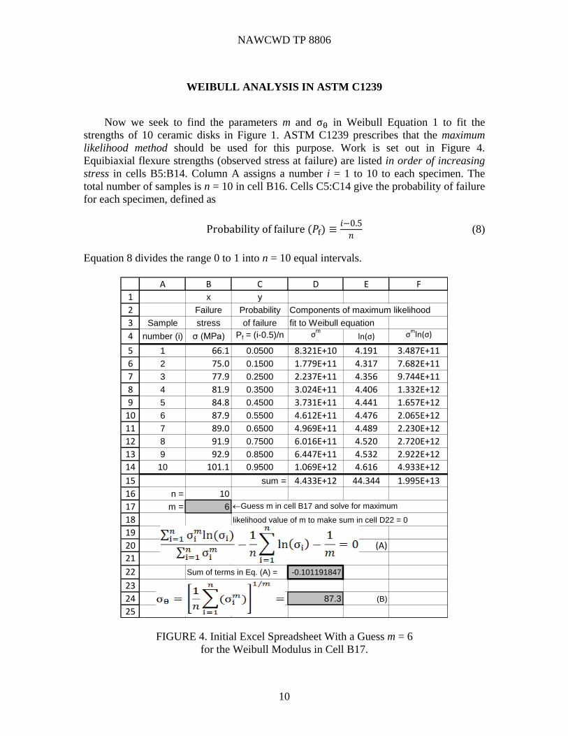
WEIBULL ANALYSIS IN ASTM C1239
Now we seek to find the parameters m and σθ in Weibull Equation 1 to fit the
strengths of 10 ceramic disks in Figure 1. ASTM C1239 prescribes that the maximum
likelihood method should be used for this purpose. Work is set out in Figure 4.
Equibiaxial flexure strengths (observed stress at failure) are listed in order of increasing
stress in cells B5:B14. Column A assigns a number i = 1 to 10 to each specimen. The
total number of samples is n = 10 in cell B16. Cells C5:C14 give the probability of failure
for each specimen, defined as
Probability of failure (𝑃f) ≡𝑖−0.5
𝑛 (8)
Equation 8 divides the range 0 to 1 into n = 10 equal intervals.
FIGURE 4. Initial Excel Spreadsheet With a Guess m = 6
for the Weibull Modulus in Cell B17.
1
2
3
4
5
6
7
8
9
10
11
12
13
14
15
16
17
18
19
20
21
22
23
24
25
A B C D E F
x y
Failure Probability Components of maximum likelihood
Sample stress of failure fit to Weibull equation
number (i) σ (MPa) Pf = (i-0.5)/n σmln(σ) σmln(σ)
1 66.1 0.0500 8.321E+10 4.191 3.487E+11
2 75.0 0.1500 1.779E+11 4.317 7.682E+11
3 77.9 0.2500 2.237E+11 4.356 9.744E+11
4 81.9 0.3500 3.024E+11 4.406 1.332E+12
5 84.8 0.4500 3.731E+11 4.441 1.657E+12
6 87.9 0.5500 4.612E+11 4.476 2.065E+12
7 89.0 0.6500 4.969E+11 4.489 2.230E+12
8 91.9 0.7500 6.016E+11 4.520 2.720E+12
9 92.9 0.8500 6.447E+11 4.532 2.922E+12
10 101.1 0.9500 1.069E+12 4.616 4.933E+12
sum = 4.433E+12 44.344 1.995E+13
n = 10
m = 6 Guess m in cell B17 and solve for maximum
likelihood value of m to make sum in cell D22 = 0
(A)
Sum of terms in Eq. (A) = -0.101191847
87.3 (B)
NAWCWD TP 8806
11
The maximum likelihood method outlined near the end of this report provides a pair
of equations that we solve for m and σθ in the spreadsheet:
Maximum likelihood equations:
∑ σi
𝑚ln(σi)𝑛i=1
∑ σi𝑚𝑛
i=1
−1
𝑛∑ ln(σi) −
1
𝑚𝑛i=1 = 0 (9)
σθ = [1𝑛
∑ (σi𝑚
)𝑛i=1 ]
1/𝑚 (10)
The spreadsheet in Figure 4 begins with a guess of the value m = 6 for the Weibull
modulus in cell B17. The guess does not have to be good for the spreadsheet to work.
With the guess m = 6, Excel computes the quantities σ𝑚, ln σ, and σ𝑚 ln σ in columns D
through F and sums in row 15. If we had guessed the correct value of m, the sum in
Equation 9 would be 0. Instead, inserting sums from row 15 into Equation 9 gives
∑ σi
𝑚ln(σi)𝑛i=1
∑ σi𝑚𝑛
i=1
−1
𝑛∑ ln(σi) −
1
𝑚
𝑛i=1 =
1.995×10¹³
4.433×10¹²−
1
10(44.344) −
1
6= −0.10119 (9)
The guess m = 6 gives a sum of ‒0.10119 for Equation 9 in cell D22.
You can use either of two Excel procedures, Solver or Goal Seek, to vary m in cell
B17 until the sum in cell D22 is 0, giving m = 10.280, which, in turn, gives the
characteristic strength σθ = 89.0 MPa from Equation 10 in cell D24 of Figure 5.
The value σθ = 89.0 MPa is considered to be a good estimate. However, there is
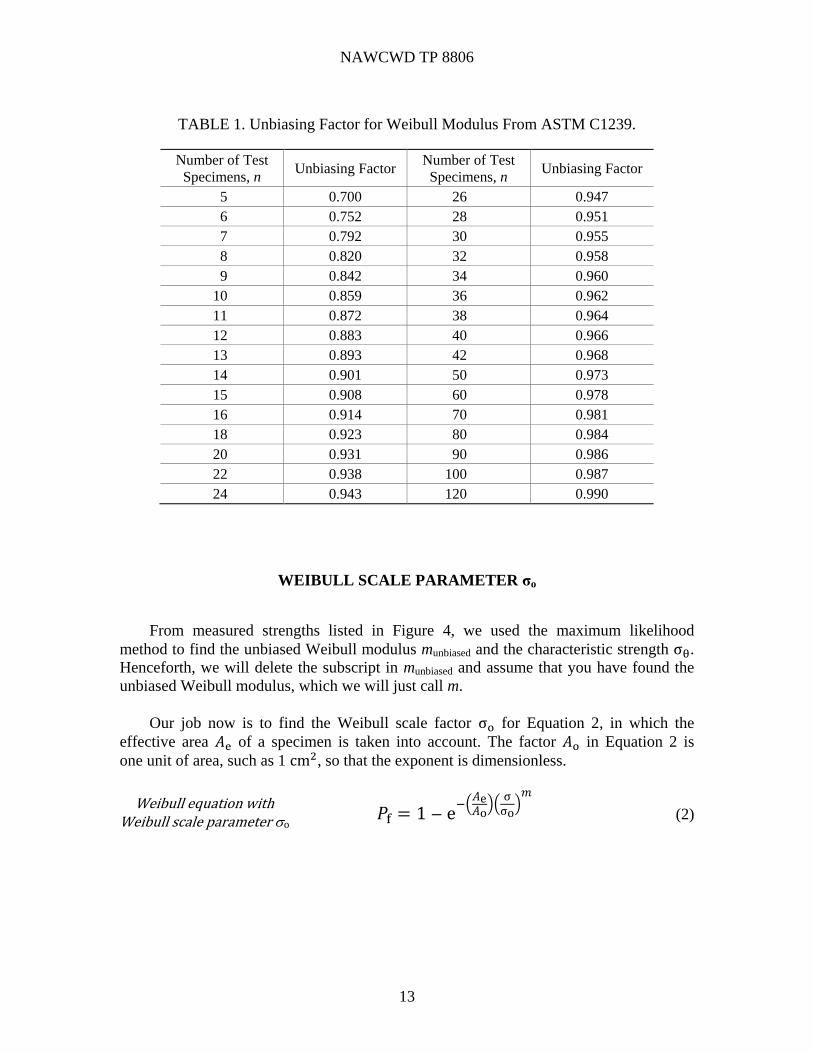
statistical bias in the value of m for small data sets (References 5 and 6). ASTM C1239
instructs us to multiply the value of m from the maximum likelihood method by the
unbiasing factor in Table 1 for the best estimate of the Weibull modulus:
𝑚𝑢nbiased = 𝑚 × 𝑢𝑛𝑏𝑖𝑎𝑠𝑖𝑛𝑔 𝑓𝑎𝑐𝑡𝑜𝑟 (11)
For n = 10 test specimens in Table 1, the unbiasing factor is 0.859, so the unbiased
estimate of m is
𝑚𝑢nbiased = 10.280 × 0.859 = 8.83 (12)
The unbiasing factor approaches 1 as the number of specimens becomes large.
According to ASTM C1239, the “best” value of m is 8.83.

NAWCWD TP 8806
12
FIGURE 5. Excel Spreadsheet After Solver Has Found m = 10.28 for the Weibull
Modulus in Cell B17 to Make the Sum in Cell D22 Zero.
1
2
3
4
5
6
7
8
9
10
11
12
13
14
15
16
17
18
19
20
21
22
23
24
25
A B C D E F
x y
Failure Probability Components of maximum likelihood
Sample stress of failure fit to Weibull equation
number (i) σ (MPa) Pf = (i-0.5)/n σmln(σ) σmln(σ)
1 66.1 0.0500 5.128E+18 4.191 2.149E+19
2 75.0 0.1500 1.886E+19 4.317 8.141E+19
3 77.9 0.2500 2.791E+19 4.356 1.216E+20
4 81.9 0.3500 4.679E+19 4.406 2.061E+20
5 84.8 0.4500 6.704E+19 4.441 2.977E+20
6 87.9 0.5500 9.643E+19 4.476 4.316E+20
7 89.0 0.6500 1.096E+20 4.489 4.918E+20
8 91.9 0.7500 1.520E+20 4.520 6.873E+20
9 92.9 0.8500 1.711E+20 4.532 7.756E+20
10 101.1 0.9500 4.068E+20 4.616 1.878E+21
sum = 1.102E+21 44.344 4.992E+21
n = 10
m = 10.28001 Guess m in cell B17 and solve for maximum
likelihood value of m to make sum in cell D22 = 0
(A)
Sum of terms in Eq. (A) = 3.64986E-14
89.0 (B)
NAWCWD TP 8806
13
TABLE 1. Unbiasing Factor for Weibull Modulus From ASTM C1239.
Number of Test
Specimens, n Unbiasing Factor
Number of Test
Specimens, n Unbiasing Factor
5 0.700 26 0.947
6 0.752 28 0.951
7 0.792 30 0.955
8 0.820 32 0.958
9 0.842 34 0.960
10 0.859 36 0.962
11 0.872 38 0.964
12 0.883 40 0.966
13 0.893 42 0.968
14 0.901 50 0.973
15 0.908 60 0.978
16 0.914 70 0.981
18 0.923 80 0.984
20 0.931 90 0.986
22 0.938 100 0.987
24 0.943 120 0.990
WEIBULL SCALE PARAMETER σo
From measured strengths listed in Figure 4, we used the maximum likelihood
method to find the unbiased Weibull modulus munbiased and the characteristic strength σθ.
Henceforth, we will delete the subscript in munbiased and assume that you have found the
unbiased Weibull modulus, which we will just call m.
Our job now is to find the Weibull scale factor σo for Equation 2, in which the
effective area 𝐴e of a specimen is taken into account. The factor 𝐴o in Equation 2 is
one unit of area, such as 1 cm2, so that the exponent is dimensionless.
Weibull equation withWeibull scale parameter o
𝑃f = 1 − e−(
𝐴e𝐴o
)(σ
σo)
𝑚
(2)
NAWCWD TP 8806
14
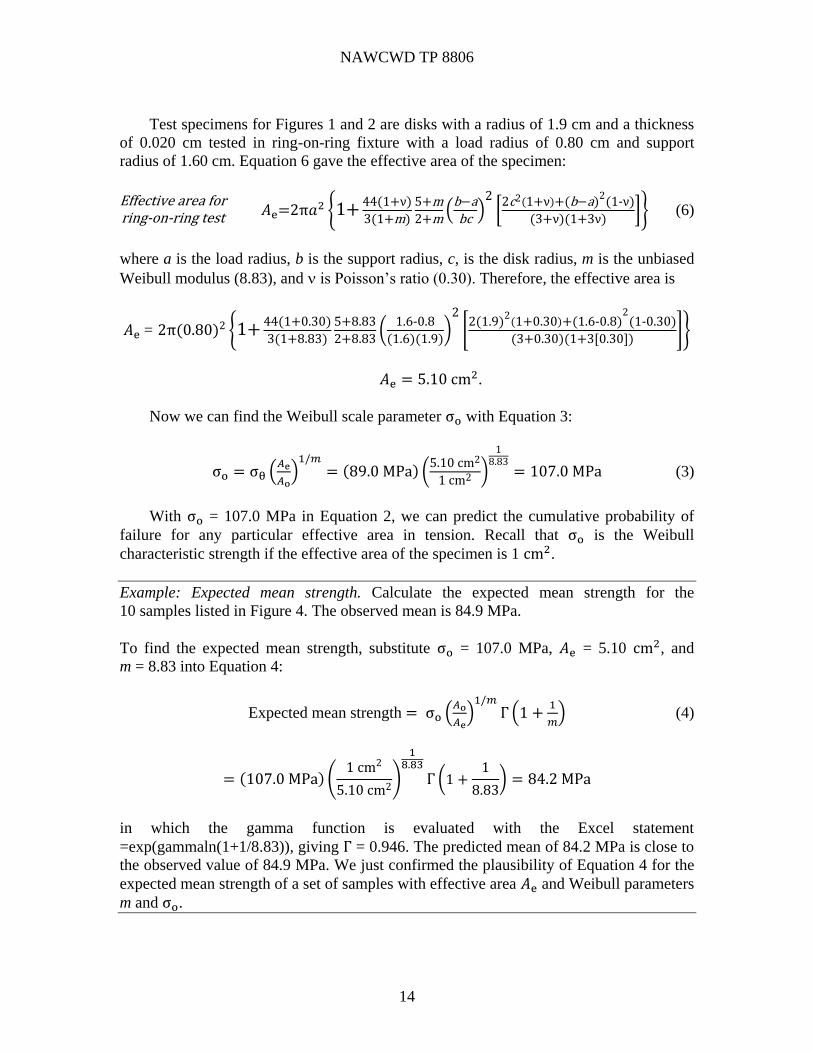
Test specimens for Figures 1 and 2 are disks with a radius of 1.9 cm and a thickness
of 0.020 cm tested in ring-on-ring fixture with a load radius of 0.80 cm and support
radius of 1.60 cm. Equation 6 gave the effective area of the specimen:
Effective area forring-on-ring test 𝐴e=2π𝑎2 {1+
44(1+ν)
3(1+m)
5+m2+m
(b−abc
)2
[2c2(1+ν)+(b−a)
2(1-ν)
(3+ν)(1+3ν)]} (6)
where a is the load radius, b is the support radius, c, is the disk radius, m is the unbiased
Weibull modulus (8.83), and is Poisson’s ratio (0.30). Therefore, the effective area is
𝐴e = 2π(0.80)2 {1+44(1+0.30)
3(1+8.83)
5+8.83
2+8.83(
1.6-0.8
(1.6)(1.9))
2
[2(1.9)
2(1+0.30)+(1.6-0.8)
2(1-0.30)
(3+0.30)(1+3[0.30])]}
𝐴e = 5.10 cm2.
Now we can find the Weibull scale parameter σo with Equation 3:
σo = σθ (𝐴e
𝐴o)
1/𝑚= (89.0 MPa) (
5.10 cm2
1 cm2 )
18.83
= 107.0 MPa (3)
With σo = 107.0 MPa in Equation 2, we can predict the cumulative probability of
failure for any particular effective area in tension. Recall that σo is the Weibull
characteristic strength if the effective area of the specimen is 1 cm2.
Example: Expected mean strength. Calculate the expected mean strength for the
10 samples listed in Figure 4. The observed mean is 84.9 MPa.
To find the expected mean strength, substitute σo = 107.0 MPa, 𝐴e = 5.10 cm2, and
m = 8.83 into Equation 4:
Expected mean strength = σo (𝐴o
𝐴e)
1/𝑚Γ (1 +
1
𝑚) (4)
= (107.0 MPa) (1 cm2
5.10 cm2)
18.83
Γ (1 +1
8.83) = 84.2 MPa
in which the gamma function is evaluated with the Excel statement
=exp(gammaln(1+1/8.83)), giving Γ = 0.946. The predicted mean of 84.2 MPa is close to
the observed value of 84.9 MPa. We just confirmed the plausibility of Equation 4 for the
expected mean strength of a set of samples with effective area 𝐴e and Weibull parameters
m and σo.
NAWCWD TP 8806
15
STRENGTH SCALES WITH AREA UNDER STRESS
The larger the area of a ceramic, the lower the strength because the probability of
finding a large flaw is greater in a large area. A slightly rewritten form of Equation 3
relates the expected mean strength 𝑆2 for specimens with effective area 𝐴2 to the
observed mean strength 𝑆1 for specimens with effective area 𝐴1.
Weibull areascaling
𝑆2
𝑆1= (
𝐴1
𝐴2)
1/𝑚. (13)
If a material fails from flaws distributed throughout its volume, we would replace
areas in Equation 13 with volumes. To derive Equation 13, substitute 𝑆2 for σo, 𝑆1 for σθ,
𝐴1 for 𝐴e, and 𝐴2 for 𝐴o in Equation 3.
Example: Predicting flexure strength for components with different size. Disks for
Figure 1 with an effective area of 5.10 cm2 have an observed mean strength 𝑆1 =
84.9 MPa with a Weibull modulus of m = 8.83 and Weibull scale factor of σo =
107.0 MPa. Use Equation 4 to predict the mean strength of the same quality of material
with an effective area of 200 cm2 under tensile stress. Substituting Weibull parameters
into Equation 4 gives the prediction:
Expected mean strength = σo (𝐴o
𝐴e)
1/𝑚Γ (1 +
1
𝑚) (4)
= (107.0 MPa) (1 cm2
200 cm2)
1
8.83Γ (1 +
1
8.83) = (107.0 MPa)(0.5488)(0.9461) = 55.6 MPa
We predict that the 200-cm2 specimens will fail at a mean stress of 55.6 MPa. The
greater the Weibull modulus, the less the strength depends on area. For m = 15, we would
predict that the mean strength of the 200-cm2 specimens would be 72.6 MPa.
EXPERIMENTAL CONFIRMATION OF WEIBULL AREA SCALING
Figure 6 shows experimental data that conform to the Weibull scaling law in
Equation 13 for areas varying over a factor of 130. Taking the base 10 logarithm of both
sides of Equation 13 gives
log 𝑆2 = −1
𝑚log (
𝐴2
𝐴1) + log 𝑆1 (14)
NAWCWD TP 8806
16
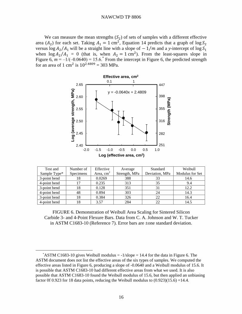
We can measure the mean strengths (𝑆2) of sets of samples with a different effective
area (𝐴2) for each set. Taking 𝐴1 = 1 cm2, Equation 14 predicts that a graph of log 𝑆2
versus log 𝐴2 𝐴1⁄ will be a straight line with a slope of − 1 𝑚⁄ and a y-intercept of log 𝑆1
when log 𝐴2 𝐴1⁄ = 0 (that is, when 𝐴2 = 1 cm2). From the least-squares slope in
Figure 6, m = ‒1/(‒0.0640) = 15.6.* From the intercept in Figure 6, the predicted strength
for an area of 1 cm2 is 102.4809 = 303 MPa.
Test and
Sample Type*
Number of
Specimens
Effective
Area, cm2
Average
Strength, MPa
Standard
Deviation, MPa
Weibull
Modulus for Set
3-point bend 18 0.0269 388 33 14.6
4-point bend 17 0.235 313 35 9.4
3-point bend 18 0.128 351 31 12.2
4-point bend 48 0.894 303 24 14.3
3-point bend 18 0.384 326 22 16.4
4-point bend 18 3.57 284 22 14.5
FIGURE 6. Demonstration of Weibull Area Scaling for Sintered Silicon
Carbide 3- and 4-Point Flexure Bars. Data from C. A. Johnson and W. T. Tucker
in ASTM C1683-10 (Reference 7). Error bars are ±one standard deviation.
*ASTM C1683-10 gives Weibull modulus = -1/slope = 14.4 for the data in Figure 6. The
ASTM document does not list the effective areas of the six types of samples. We computed the
effective areas listed in Figure 6, producing a slope of -0.0640 and a Weibull modulus of 15.6. It
is possible that ASTM C1683-10 had different effective areas from what we used. It is also
possible that ASTM C1683-10 found the Weibull modulus of 15.6, but then applied an unbiasing
factor 0f 0.923 for 18 data points, reducing the Weibull modulus to (0.923)(15.6) =14.4.
y = -0.0640x + 2.4809
2.40
2.45
2.50
2.55
2.60
2.65
-2.0 -1.5 -1.0 -0.5 0.0 0.5 1.0
Lo
g (
av
era
ge s
tren
gth
, M
Pa)
Log (effective area, cm2)
282
316
355
398
447
251
Str
en
gth
(M
Pa)
10.1
Effective area, cm2
NAWCWD TP 8806
17
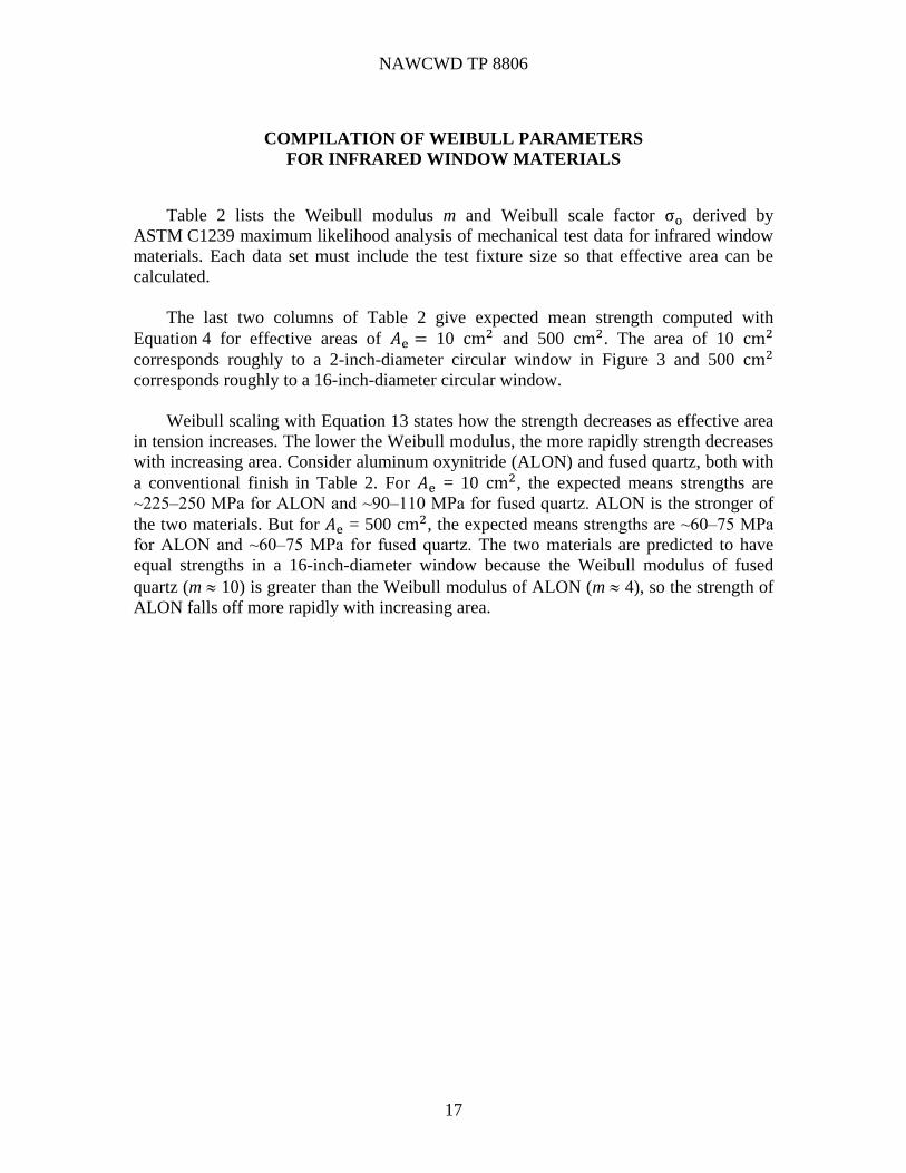
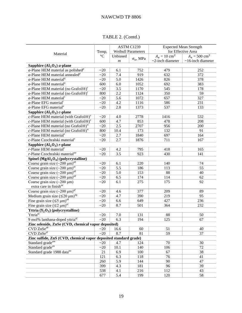
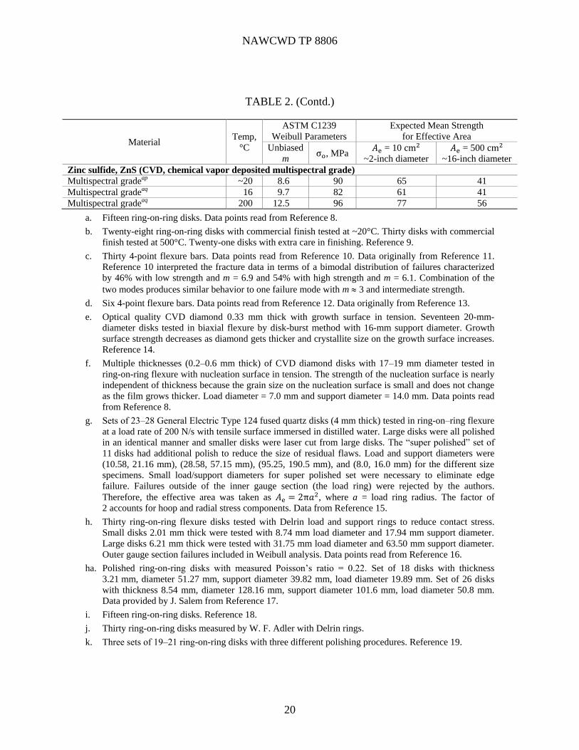
COMPILATION OF WEIBULL PARAMETERS
FOR INFRARED WINDOW MATERIALS
Table 2 lists the Weibull modulus m and Weibull scale factor σo derived by
ASTM C1239 maximum likelihood analysis of mechanical test data for infrared window
materials. Each data set must include the test fixture size so that effective area can be
calculated.
The last two columns of Table 2 give expected mean strength computed with
Equation 4 for effective areas of 𝐴e = 10 cm2 and 500 cm2. The area of 10 cm2
corresponds roughly to a 2-inch-diameter circular window in Figure 3 and 500 cm2
corresponds roughly to a 16-inch-diameter circular window.
Weibull scaling with Equation 13 states how the strength decreases as effective area
in tension increases. The lower the Weibull modulus, the more rapidly strength decreases
with increasing area. Consider aluminum oxynitride (ALON) and fused quartz, both with
a conventional finish in Table 2. For 𝐴e = 10 cm2, the expected means strengths are
~225‒250 MPa for ALON and ~90‒110 MPa for fused quartz. ALON is the stronger of
the two materials. But for 𝐴e = 500 cm2, the expected means strengths are ~60‒75 MPa
for ALON and ~60‒75 MPa for fused quartz. The two materials are predicted to have
equal strengths in a 16-inch-diameter window because the Weibull modulus of fused
quartz (m 10) is greater than the Weibull modulus of ALON (m 4), so the strength of
ALON falls off more rapidly with increasing area.

NAWCWD TP 8806
18
TABLE 2. Strengths of Infrared Window Materials: ASTM C1239 Weibull Parameters.
Material Temp,
°C
ASTM C1239
Weibull Parameters
Expected Mean Strength
for Effective Area
Unbiased
m σo, MPa
𝐴e = 10 cm2
~2-inch diameter
𝐴e = 500 cm2
~16-inch diameter
Aluminum oxynitride, 9𝐀𝐥𝟐𝐎𝟑 ∙ ~𝟑. 𝟔𝐀𝐥𝐍 (polycrystalline ALON)
Manufacturer 1a ~20 4.3 328 175 70
Manufacturer 2 commercial finishb ~20 2.9 559 225 58
Manufacturer 2 commercial finishb 500 3.2 577 252 74
Manufacturer 2 extra care in finishingb ~20 4.1 828 429 165
Calcium fluoride, 𝐂𝐚𝐅𝟐
Fusion cast polycrystalline CaF2c ~20 3.1 111 47 13
Single crystal (111) CaF2d ~20 2.8 83 32 8
Diamond (CVD, chemical vapor deposited thick film) (polycrystalline)
Manufacturer 1 optical gradee ~20 7.4 442 304 179
Manufacturer 2f ~20 2.8 520 203 50
Fused quartz, 𝐒𝐢𝐎𝟐 (similar to fused silica) immersed in water
25.4-mm-diameter disksg 20 10.8 120 93 64
76.2-mm-diameter disksg 20 11.0 135 105 73
228.6-mm-diameter disksg 20 7.4 162 111 66
25.4-mm-diam. disks, superpolishedg 20 9.4 180 134 88
Germanium, Ge (polycrystalline)
20.0-mm-diameter disksh ~20 4.4 179 97 40
76.2-mm-diameter disksh ~20 4.5 237 130 54
128-mm-diameter disksha 20 5.6 341 222 104
51-mm-diameter disksha 23 6.4 291 189 103
Magnesium fluoride, 𝐌𝐠𝐅𝟐 (polycrystalline)
Hot pressed U.S. material from 1970si ~20 4.4 218 118 48
Hot pressed French material from
1990sj
~20 3.3 190 85 26
Single crystalk ~20 ~4.9 ~160 ~92 ~41
Hot pressed U.S. material from 1970sl 24 8.4 113 81 51
121 15 121 100 77
260 10.8 120 93 64
399 5.6 107 66 33
538 4.9 86 49 22
Nanocomposite optical ceramic (MgO:𝐘𝟐𝐎𝟑 50:50 vol:vol)
38-mm-diameter disksm 21 6.8 819 545 307
38-mm-diameter disksn 600 5.8 580 361 184
Polycrystalline alumina (𝐀𝐥𝟐𝐎𝟑) (infrared-transparent material with grain size 0.3‒0.4 μm)
2008 data seto 24 6.3 1352 873 459
2016 data seto 21 11.8 867 683 490
2016 data seto 500 11.6 758 595 425
2016 data seto 750 11.9 715 564 406
2016 data seto 1000 10.3 672 512 350
NAWCWD TP 8806
19
TABLE 2. (Contd.)
Material Temp,
°C
ASTM C1239
Weibull Parameters
Expected Mean Strength
for Effective Area
Unbiased
m σo, MPa
𝐴e = 10 cm2
~2-inch diameter
𝐴e = 500 cm2
~16-inch diameter
Sapphire (𝐀𝐥𝟐𝐎𝟑) a-plane
a-Plane HEM material as polishedp ~20 6.1 752 479 252
a-Plane HEM material annealedp ~20 7.4 919 632 372
a-Plane HEM materialq ~20 5.0 1426 826 378
a-Plane HEM materialq 600 6.0 1052 692 383
a-Plane HEM material (no Grafoil®)r ~20 3.5 1170 545 178
a-Plane HEM material (no Grafoil®)r 800 2.2 1124 350 59
a-Plane HEM materials ~20 5.6 1072 657 327
a-Plane EFG materialt ~20 4.2 1116 586 231
a-Plane EFG materialu ~20 2.8 1373 537 133
Sapphire (𝐀𝐥𝟐𝐎𝟑) c-plane
c-Plane HEM material (with Grafoil®)v ~20 4.0 2778 1416 532
c-Plane HEM material (with Grafoil®)v 600 4.7 853 478 208
c-Plane HEM material (no Grafoil®)w ~20 2.5 2707 956 200
c-Plane HEM material (no Grafoil®)w 800 10.4 173 132 91
c-Plane HEM materialx ~20 2.7 1840 697 164
c-Plane Czochralski materialy ~20 2.7 1876 711 167
Sapphire (𝐀𝐥𝟐𝐎𝟑) r-plane
r-Plane HEM materialz ~20 4.2 795 418 165
r-Plane Czochralski materialaa ~20 3.5 923 430 141
Spinel (𝐌𝐠𝐀𝐥𝟐𝐎𝟒) (polycrystalline)
Coarse grain size (~200 μm)ab ~20 6.1 220 140 74
Coarse grain size (~200 μm)ac ~20 5.5 186 113 55
Coarse grain size (~200 μm)ah ~20 5.0 153 88 40
Coarse grain size (~200 μm)ad ~20 6.5 174 114 62
Coarse grain size (~200 μm)
extra care in finishae
~20 6.1 275 175 92
Coarse grain size (~200 μm)af ~20 4.6 377 209 89
Medium grain size (≲20 μm)ag ~20 4.7 390 219 95
Fine grain size (≲5 μm)ah ~20 6.6 649 427 236
Fine grain size (≲2 μm)ai ~20 8.7 501 364 232
Yttria (𝐘𝟐𝐎𝟑) (polycrystalline)
Yttriaaj ~20 7.0 131 88 50
9 mol% lanthana-doped yttriaaj ~20 6.3 194 125 67
Zinc selenide, ZnSe (CVD, chemical vapor deposited)
CVD ZnSeak ~20 16.6 60 51 40
CVD ZnSeal ~20 8.7 81 59 37
Zinc sulfide, ZnS (CVD, chemical vapor deposited standard grade)
Standard gradeam ~20 4.7 124 70 30
Standard gradean ~20 10.1 140 106 72
Standard grade 1988 dataao 21 6.9 100 67 38
121 6.3 118 76 41
260 5.9 144 90 47
399 4.3 181 96 39
538 4.1 216 112 43
677 5.4 199 120 58
NAWCWD TP 8806
20
TABLE 2. (Contd.)
Material Temp,
°C
ASTM C1239
Weibull Parameters
Expected Mean Strength
for Effective Area
Unbiased
m σo, MPa
𝐴e = 10 cm2
~2-inch diameter
𝐴e = 500 cm2
~16-inch diameter
Zinc sulfide, ZnS (CVD, chemical vapor deposited multispectral grade)
Multispectral gradeap ~20 8.6 90 65 41
Multispectral gradeaq 16 9.7 82 61 41
Multispectral gradeaq 200 12.5 96 77 56
a. Fifteen ring-on-ring disks. Data points read from Reference 8.
b. Twenty-eight ring-on-ring disks with commercial finish tested at ~20°C. Thirty disks with commercial
finish tested at 500°C. Twenty-one disks with extra care in finishing. Reference 9.
c. Thirty 4-point flexure bars. Data points read from Reference 10. Data originally from Reference 11.
Reference 10 interpreted the fracture data in terms of a bimodal distribution of failures characterized
by 46% with low strength and m = 6.9 and 54% with high strength and m = 6.1. Combination of the
two modes produces similar behavior to one failure mode with m 3 and intermediate strength.
d. Six 4-point flexure bars. Data points read from Reference 12. Data originally from Reference 13.
e. Optical quality CVD diamond 0.33 mm thick with growth surface in tension. Seventeen 20-mm-
diameter disks tested in biaxial flexure by disk-burst method with 16-mm support diameter. Growth
surface strength decreases as diamond gets thicker and crystallite size on the growth surface increases.
Reference 14.
f. Multiple thicknesses (0.2‒0.6 mm thick) of CVD diamond disks with 17‒19 mm diameter tested in
ring-on-ring flexure with nucleation surface in tension. The strength of the nucleation surface is nearly
independent of thickness because the grain size on the nucleation surface is small and does not change
as the film grows thicker. Load diameter = 7.0 mm and support diameter = 14.0 mm. Data points read
from Reference 8.
g. Sets of 23‒28 General Electric Type 124 fused quartz disks (4 mm thick) tested in ring-on–ring flexure
at a load rate of 200 N/s with tensile surface immersed in distilled water. Large disks were all polished
in an identical manner and smaller disks were laser cut from large disks. The “super polished” set of
11 disks had additional polish to reduce the size of residual flaws. Load and support diameters were
(10.58, 21.16 mm), (28.58, 57.15 mm), (95.25, 190.5 mm), and (8.0, 16.0 mm) for the different size
specimens. Small load/support diameters for super polished set were necessary to eliminate edge
failure. Failures outside of the inner gauge section (the load ring) were rejected by the authors.
Therefore, the effective area was taken as 𝐴e = 2π𝑎2, where a = load ring radius. The factor of
2 accounts for hoop and radial stress components. Data from Reference 15.
h. Thirty ring-on-ring flexure disks tested with Delrin load and support rings to reduce contact stress.
Small disks 2.01 mm thick were tested with 8.74 mm load diameter and 17.94 mm support diameter.
Large disks 6.21 mm thick were tested with 31.75 mm load diameter and 63.50 mm support diameter.
Outer gauge section failures included in Weibull analysis. Data points read from Reference 16.
ha. Polished ring-on-ring disks with measured Poisson’s ratio = 0.22. Set of 18 disks with thickness
3.21 mm, diameter 51.27 mm, support diameter 39.82 mm, load diameter 19.89 mm. Set of 26 disks
with thickness 8.54 mm, diameter 128.16 mm, support diameter 101.6 mm, load diameter 50.8 mm.
Data provided by J. Salem from Reference 17.
i. Fifteen ring-on-ring disks. Reference 18.
j. Thirty ring-on-ring disks measured by W. F. Adler with Delrin rings.
k. Three sets of 19‒21 ring-on-ring disks with three different polishing procedures. Reference 19.
NAWCWD TP 8806
21
l. Four-point flexure bars; length = 25.4 mm, thickness = width = 1.78 mm, load span = 8.38 mm,
support span = 16.76 mm. Number of specimens at each temperature: 24°C, n = 20; 121°C, n = 9;
260°C, n = 15; 399°C, n = 18; 538°C, n = 16.
m. Fourteen ring-on-ring disks. Reference 20.
n. Sixteen ring-on-ring disks. Reference 20. Weibull parameters in the table are derived by omitting the
two strongest specimens from 18 disks tested. If all 18 results are used, derived parameters are m = 3.6
and σo = 700 MPa, giving predicted strengths of 333 and 184 MPa for 𝐴e = 10 and 500 cm2,
respectively. Discarding the two strongest samples increases the apparent Weibull modulus and
predicts greater strength for large windows.
o. Twenty-three to 30 ring-on-ring disks. References 21, 22, and 23.
p. HEM = heat exchanger method. Fourteen ring-on-ring disks. Reference 24. Annealing conditions are
not stated, but it has been shown that annealing near 1200C in air strengthens sapphire by healing
some polishing damage (Reference 25).
q. HEM = heat exchanger method. Ten ring-on-ring disk. Reference 26.
r. HEM = heat exchanger method. No Grafoil® was used between specimen and test fixture. Twenty
ring-on-ring disks at ~20C and 22 disks at 800C. References 27 and 28.
s. HEM = heat exchanger method. Eleven ring-on-ring disks.
t. EFG = edge-defined film-fed growth method. Nine ring-on-ring disks.
u. EFG = edge-defined film-fed growth method. Twenty six ring-on-ring disks.
v. HEM = heat exchanger method. Eight ring-on-ring disks at ~20C and 11 disks at 600C.
Reference 26.
w. HEM = heat exchanger method. No Grafoil® was used between specimen and test fixture. Twenty
ring-on-ring disks at ~20C and at 800C. References 27 and 28.
x. HEM = heat exchanger method. Eight ring-on-ring disks. Data points read from Reference 8.
y. Czochralski crystal growth. Eight ring-on-ring disk. Data points read from Reference 8.
z. HEM = heat exchanger method. Twelve ring-on-ring disks. Data points read from Reference 8.
aa. Czochralski crystal growth. Six ring-on-ring disks. Data points read from Reference 8.
ab. Ten ring-on-ring disk taken from 23-mm-thick plate.
ac. Twenty-three ring-on-ring disks taken from a large plate.
ad. Fourteen ring-on-ring disks taken from a large plate.
ae. Twenty-one ring-on-ring disks taken from a large plate.
af. Twenty-seven ring-on-ring disks taken from a large plate.
ag. Fifteen ring-on-ring disks.
ah. Fifteen ring-on-ring disks.
ai. Seventeen ring-on-ring disks. From Reference 29. Data courtesy S. Sweeney.
aj. Materials produced in 1987. Forty ring-on-ring disks. References 30, 31, and 32.
ak. Twenty ring-on-ring disks. Data points read from Reference 8.
al. Fifteen ring-on-ring disks tested in distilled water at 10.2 MPa/s. Data from Reference 33.
am. Thirteen ring-on-ring disks.
an. Twenty ring-on-ring disks. Data points read Reference 8.
ao. Twenty ring-on-ring disks. Data from Reference 34.
ap. Twenty ring-on-ring disks. Data points read from Reference 8.
aq. ASTM C1161Size C 4-point flexure bars: 24 bars at 16°C and 23 bars at 200°C. Reference 35.

NAWCWD TP 8806
22
WEIBULL PROBABILITY OF SURVIVAL WITHOUT
SLOW CRACK GROWTH
How can we use the Weibull equation to predict the probability of survival of a
window made from a material whose strength we have measured with coupons? Consider
the transparent polycrystalline alumina window in Figure 7 held in a frame by a
compliant gasket with a pressure difference P = 0.5 MPa (5 bar) across the window. The
right side of the window becomes convex and is placed in tension. The maximum stress
at the center of the tensile face computed with Equations 15 and 16 (Reference 4) is
364.8 MPa. Poisson’s ratio and Young’s modulus given in the figure caption apply to a
fine-grain polycrystalline alumina (grain size 0.3‒0.4 μm) that is transparent in the
midwave infrared region and visibly translucent (References 22, 36 through 40).
FIGURE 7. Window in a Frame With Pressure Difference P = 0.5 MPa Across the
Window. Window radius c = 55 mm, support radius (gasket radius) b = 50 mm,
window thickness d = 2.0 mm, Poisson’s ratio = 0.24,
and Young’s modulus E = 403 GPa.
Radial stress = 3𝑃𝑏2
8𝑑2[(1 − 𝜈) (
𝑏2
𝑐2) + 2(1 + 𝜈) − (3 + 𝜈) (
𝑟2
𝑏2)] +
(3+ν)𝑃
4(1−ν) (15)
Hoop stress = 3𝑃𝑏2
8𝑑2[(1 − 𝜈) (
𝑏2
𝑐2) + 2(1 + 𝜈) − (1 + 3𝜈) (
𝑟2
𝑏2)] +
(3+ν)𝑃
4(1−ν) (16)
where r is the radial location measured from the center of the window, b is the radius of
the gasket ring (Figure 3), c is disk radius, d is disk thickness, is Poisson’s ratio, and
P is the pressure difference between the two surfaces.
0
50
100
150
200
250
300
350
400
0 10 20 30 40 50
Str
ess
(M
Pa
)
Radial distance (mm)
Hoop stress
Radial stress
Polycrystalline aluminawindow stress
NAWCWD TP 8806
23
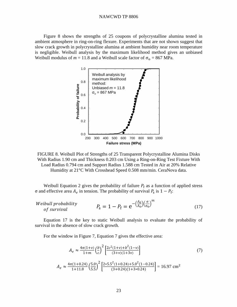
Figure 8 shows the strengths of 25 coupons of polycrystalline alumina tested in
ambient atmosphere in ring-on-ring flexure. Experiments that are not shown suggest that
slow crack growth in polycrystalline alumina at ambient humidity near room temperature
is negligible. Weibull analysis by the maximum likelihood method gives an unbiased
Weibull modulus of m = 11.8 and a Weibull scale factor of σo = 867 MPa.
FIGURE 8. Weibull Plot of Strengths of 25 Transparent Polycrystalline Alumina Disks
With Radius 1.90 cm and Thickness 0.203 cm Using a Ring-on-Ring Test Fixture With
Load Radius 0.794 cm and Support Radius 1.588 cm Tested in Air at 20% Relative
Humidity at 21°C With Crosshead Speed 0.508 mm/min. CeraNova data.
Weibull Equation 2 gives the probability of failure 𝑃f as a function of applied stress
σ and effective area 𝐴𝑒 in tension. The probability of survival 𝑃s is 1 − 𝑃f:
𝑊𝑒𝑖𝑏𝑢𝑙𝑙 𝑝𝑟𝑜𝑏𝑎𝑏𝑖𝑙𝑖𝑡𝑦𝑜𝑓 𝑠𝑢𝑟𝑣𝑖𝑣𝑎𝑙
𝑃s = 1 − 𝑃f = e−(
𝐴e𝐴o
)(σ
σo)
𝑚
(17)
Equation 17 is the key to static Weibull analysis to evaluate the probability of
survival in the absence of slow crack growth.
For the window in Figure 7, Equation 7 gives the effective area:
𝐴𝑒 ≈4𝜋(1+𝜈)
1+𝑚(
𝑏
𝑐)
2[
2𝑐2(1+𝜈)+𝑏2
(1−𝜈)
(3+𝜈)(1+3𝜈)] (7)
𝐴𝑒 ≈4𝜋(1+0.24)
1+11.8(
5.0
5.5)
2[
2∗5.52
(1+0.24)+5.02
(1−0.24)
(3+0.24)(1+3∗0.24)] = 16.97 cm2
0.0
0.2
0.4
0.6
0.8
1.0
200 300 400 500 600 700 800 900 1000
Pro
ba
bil
ity o
f fa
ilu
re
Failure stress (MPa)
PCA 21 C
fit
CeraNva PCA 21 C 2016(maximum likelihood)
Weibull analysis by maximum likelihood method:Unbiased m = 11.8σo = 867 MPa
NAWCWD TP 8806
24
Substituting Ae = 16.97 cm2 into Equation 17 predicts the probability of survival:
𝑃s = e−(
𝐴e𝐴o
)(σ
σo)
𝑚
= e−(
16.97 cm2
1 cm2 )(364.8 MPa867 MPa
)11.8
= 0.999380 (18)
The window has a 99.94% probability of survival or a probability of failure of 𝑃f = 1 −𝑃s= 1 ‒ 0.9994 = 0.06%.
For some purposes, we desire a lower probability of failure. We can decrease the
probability of failure by reducing tensile stress with a thicker window. Different values of
thickness in Equation 15 give the following stresses and probabilities of failure:
Thickness d,
mm
Maximum Stress,
MPa
Probability of Failure
𝑃f
1.5 648.1 0.42
1.75 476.3 0.014
2.0 364.8 0.0006
2.25 288.3 0.00004
2.5 233.6 0.000003
Window thickness is the principal handle available for obtaining an acceptable
probability of failure.
GENERAL APPROACH TO WEIBULL
PROBABILITY OF SURVIVAL
In the previous section, we used the effective area of the window to compute the
probability of survival with Equation 17. In many situations, we do not have closed-form
equations for stress or effective area. Commonly, a finite element analysis produces a
map of the principal stresses in each element of surface area (or volume) of a window or
dome that might have a complex shape.
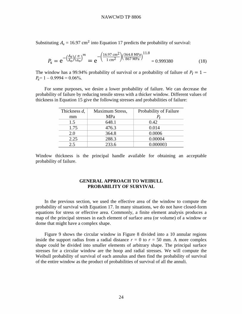
Figure 9 shows the circular window in Figure 8 divided into a 10 annular regions
inside the support radius from a radial distance r = 0 to r = 50 mm. A more complex
shape could be divided into smaller elements of arbitrary shape. The principal surface
stresses for a circular window are the hoop and radial stresses. We will compute the
Weibull probability of survival of each annulus and then find the probability of survival
of the entire window as the product of probabilities of survival of all the annuli.
NAWCWD TP 8806
25
FIGURE 9. Computing Weibull Probability of Survival by Dividing a Window Into
Many Surface Elements and Computing the Probability of Survival of Each Element.
Overall probability of survival is the product of probabilities
of survival for each element.
Consider the shaded annulus extending from 𝑟1 = 20 to 𝑟2 = 25 mm. The geometric
area of the annulus is 𝐴 = 𝜋𝑟22 − 𝜋𝑟1
2 = 0.7069 cm2. Table 3 lists the following stresses
computed with Equation 16:
Hoop stress at r = 20 mm: 332.5 MPa Average hoop stress =
Hoop stress at r = 25 mm: 314.4 MPa 1
2(332.5 + 314.4) = 323.4 MPa
Table 3 shows the average radial stress in the same annulus to be 286.9 MPa.
The probability of survival of the annulus is the product of the Weibull probabilities
of survival from the hoop and radial stresses computed from the geometric area of the
annulus with Equation 17:
𝑃s(hoop) = e−(
𝐴e𝐴o
)(σ
σo)
𝑚
= e−(
0.7069 cm2
1 cm2 )(323.4 MPa867 MPa
)11.8
= 0.999937
𝑃s(radial) = e−(
𝐴e𝐴o
)(σ
σo)
𝑚
= e−(
0.7069 cm2
1 cm2 )(286.9 MPa1352 MPa
)11.8
= 0.999985
𝑃s(𝑎𝑛𝑛𝑢𝑙𝑢𝑠) = 𝑃s(ℎ𝑜𝑜𝑝) × 𝑃s(𝑟𝑎𝑑𝑖𝑎𝑙) = (0.999937)(0.999985) = 0.999922
The probability of survival of the shaded annulus is 0.999922.

NAWCWD TP 8806
26
TABLE 3. Weibull Probability of Survival of a Window Found
From the Stress in Each Element of Area.
Radial
Distance,
mm
Hoop
Stress,
MPa
Radial
Stress,
MPa
Annular
Area,
mm2
Mean
Hoop
Stress,
MPa
Hoop
Probability
of Survival
Ps
Mean
Radial
Stress,
MPa
Radial
Probability
of Survival
Ps
0 364.8 364.8 --- --- --- --- ---
5 362.7 361.0 78.5 363.8 0.999972 362.9 0.999973
10 356.7 349.6 235.6 359.7 0.999927 355.3 0.999937
15 346.6 330.6 392.7 351.7 0.999907 340.1 0.999937
20 332.5 304.0 549.8 339.6 0.999914 317.3 0.999961
25 314.4 269.8 706.9 323.4 0.999937 286.9 0.999985
30 292.2 228.1 863.9 303.3 0.999964 249.0 0.999997
35 266.0 178.7 1021.0 279.1 0.999984 203.4 1.000000
40 235.8 121.8 1178.1 250.9 0.999995 150.2 1.000000
45 201.5 57.2 1335.2 218.6 0.999999 89.5 1.000000
50 163.2 -14.9 1492.3 182.3 1.000000 21.1 1.000000
The probability of survival of the entire window is the product of probabilities of
survival of all 10 annuli, which is
𝑃s(window) =
(0.999972)(0.999973) × (0.999927)(0.999937) … (1.000000)(1.000000) = 0.999388 (19)
𝑃s(annulus 1) 𝑃s(annulus 2) 𝑃s(annulus 10)
This approximate method of breaking the window into multiple small areas gives us
an estimate of 𝑃𝑠 = 0.999388 for the overall probability of survival of the window. We
found the value 𝑃𝑠 = 0.999380 for the window with Equation 18 from the effective area
of the entire window. In general, there would be some difference in 𝑃𝑠 found by the two
methods. The fidelity of the approximate method is improved by breaking the object into
more small elements.
To recap, the general method for finding Weibull probability of survival is to divide
the window into small elements and compute the principal tensile stresses in each surface
element by finite element analysis. Then find the probability of survival of each surface
element with Equation 17 using the geometric area for each element and the mean
principal stresses in that element. The overall probability of survival is the product of
probabilities of survival of all the surface elements.

NAWCWD TP 8806
27
SOME CAVEATS FOR WINDOW DESIGN
The procedure in the last two sections assumes that the window has the same flaw
distribution (and therefore Weibull parameters) as the test coupons used to measure
Weibull parameters. A similar statement might be that the coupons are ground and
polished by the same methods used to make the window. Even if machining of coupons is
matched as well as possible to that of the window, it is not reasonable to expect flaw
populations to be exactly the same. Anecdotal evidence suggests that every time the same
nominal procedure is used in one shop to finish the same kinds of samples, mechanical
strength test results are different. One of many possible reasons for differing results is
that the condition of the abrasive used for grinding and polishing changes during use of
the abrasive, so the abrasive is never the same from run to run.
Another caveat is that Weibull area scaling works best if the stress state of the
window is similar to the stress state of the test coupons. We chose an example in which
the window is in a “pressure-on-ring” stress state and the test coupons are in a “ring-on-
ring” stress state, which are approximately similar conditions. The more the window
stress state differs from the coupon stress state, the less likely are predictions of
probability of survival to be meaningful.
One procedure used by designers is to calculate the 90% upper and lower confidence
limits for the Weibull parameters by using equations given in ASTM C1239. Window
performance can then be calculated with the upper and lower bound Weibull parameters
to see what range of predictions results.
The two parameter Weibull Equation 1 gives more conservative predictions of
survival than a three parameter equation in which there is a lower stress limit below
which the probability of failure is considered to be zero.
Ultimately, it is excellent practice to proof test real windows to verify at some level
of confidence that a manufactured window withstands its design conditions with some
additional margin of safety.
NAWCWD TP 8806
28
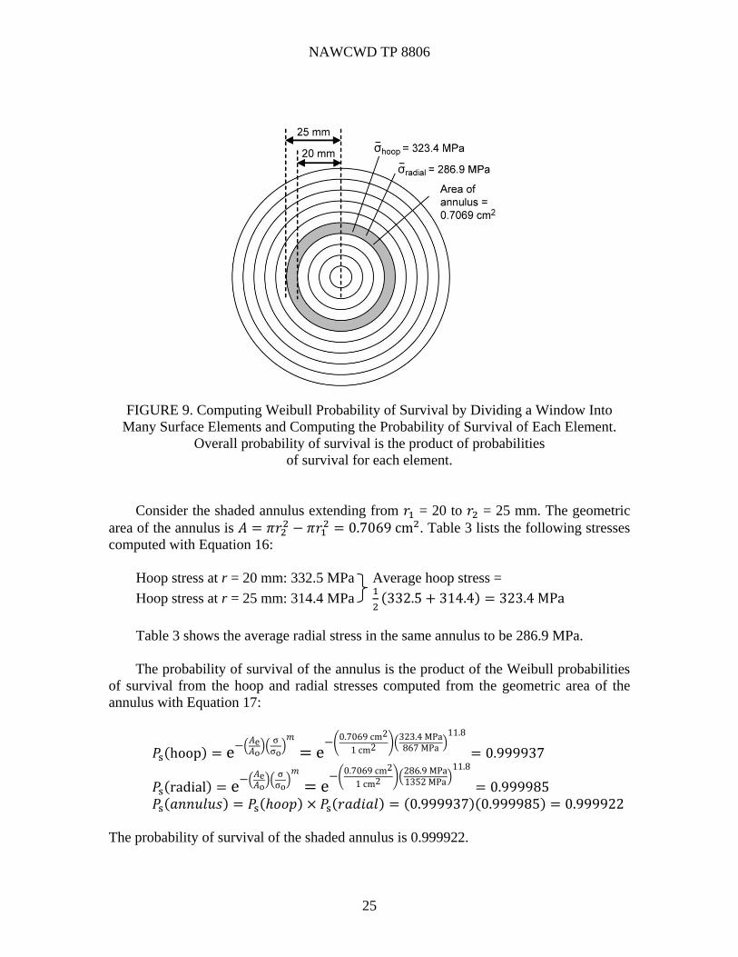
MAXIMUM LIKELIHOOD METHOD
For the Weibull cumulative probability of failure function Equation 1,
Weibull equation with
characteristic strength 𝑃f = 1 − e
−(σ
σθ)
𝑚
(1)
the probability density p is the derivative 𝑑𝑃f 𝑑σ⁄ :
Probability density 𝑝 ≡𝑑𝑃f
𝑑σ= (
𝑚
σθ) (
σ
σθ)
𝑚−1e
−(σ
σθ)
𝑚
(20)
Unlike a Gaussian probability curve, Weibull probability is not symmetric about the
peak. The maximum probability density of 0.00434 occurs at a stress of 542 MPa in
Figure 10, whereas 50% cumulative probability of failure occurs at 530 MPa.
FIGURE 10. Weibull Cumulative Probability of Failure Pf From Equation 1
and Probability Density From Equation 20 for m = 6.48 and σθ = 555.8 MPa.
Open circles are experimental data for 80 4-point flexure specimens of hot
isostatically pressed silicon carbide from Table 4 of ASTM C1239-13.
The experimental probability density for 80 flexure test specimens in Figure 10
conforms well to the dashed curve, which is the derivative of the solid line. Weibull
parameters were found by the maximum likelihood method of ASTM C1239. The
likelihood of observing experimental points is greatest at the peak of the probability
density function.
0
0.001
0.002
0.003
0.004
0.005
0.0
0.1
0.2
0.3
0.4
0.5
0.6
0.7
0.8
0.9
1.0
0 100 200 300 400 500 600 700 800
Pro
ba
bil
ity d
en
sit
y,
dP
f/d
σ
Cu
mu
lati
ve
pro
ba
bil
ity o
f fa
ilu
re,
Pf
Stress, σ (MPa)
Smooth functions
Cumulative probabilityof failure, Pf
Probabilitydensity, dPf /dσ
NAWCWD TP 8806
29
The likelihood function, ℒ, for n experimental data points is the product of
probability densities in Equation 20 for all points in the set of strength measurements:
Liklihoodfunction ℒ = ∏ 𝑝i
𝑛𝑖=1 = ∏ (
𝑚
σθ) (
σi
σθ)
𝑚−1e
−(σiσθ
)𝑚
𝑛𝑖=1 (21)
where the symbol Π stands for a product just as Σ stands for a sum. Units of the
likelihood function are 1/MPa, which means probability per megapascal.
Example: Maximum likelihood function. The spreadsheet in Figure 4 lists flexure
strengths of 10 specimens. Write the first two terms of the likelihood function using trial
Weibull parameters m = 6 and σθ = 87.3 MPa found in cells B17 and D24 of the
spreadsheet.
The first two measured strengths are 66.1 and 75.0 MPa, so the first two terms of the
likelihood product are
ℒ = ∏ (𝑚
σθ) (
σi
σθ)
𝑚−1
e−(
σiσθ
)𝑚𝑛
𝑖=1
=
[(6
87.3 MPa) (
66.1 MPa
87.3 MPa)
6−1e−(
66.1 MPa87.3 MPa
)6
] [(6
87.3 MPa) (
75.0 MPa
87.3 MPa)
6−1e−(
75.0 MPa87.3 MPa
)6
]
There would be 10 terms in the likelihood product.
The maximum likelihood method seeks values of m and 𝜎𝜃 that maximize the
likelihood function in Equation 21. With trial values m = 6 and σθ = 87.3 MPa, the
product of all 10 terms in the example above is ℒ = 1.832 × 10⁻¹⁷ (MPa)−1. The
optimum values m = 10.280 and σθ = 89.05 MPa derived in Figure 5 give the maximum
likelihood ℒ = 11.863 × 10⁻¹⁷ (MPa)−1.
To find the optimum values of m and σθ, recall that the derivative of a function is 0
at the maximum value of the function. Optimum values of m and σθ giving the maximum
value of ℒ must satisfy two simultaneous partial derivative equations of ℒ with respect to
m and σθ:
𝜕ℒ
𝜕𝑚= 0 and
𝜕ℒ
𝜕σθ= 0 (22)
It is inconvenient to write expressions for 𝜕ℒ 𝜕𝑚⁄ and 𝜕ℒ 𝜕σθ⁄ in Equation 22.
However, values of m and σθ that maximize ℒ also maximize the natural logarithm of ℒ
because ln ℒ increases monotonically as ℒ increases.
NAWCWD TP 8806
30
To find the natural logarithm of ℒ, use the identity ln 𝑎𝑏𝑐 … . = ln 𝑎 + ln 𝑏 + ln 𝑐 … . Applying this identity to the product of n terms in Equation 21, we can write a sum
instead of a product:
ln ℒ = ln 𝑝1𝑝2 ⋯ 𝑝𝑛 = ln 𝑝1 + ln 𝑝2 + ⋯ + ln 𝑝𝑛
= ln [ (𝑚
σθ) (
σ1
σθ)
𝑚−1e
−(σ1σθ
)𝑚
] + ⋯ + ln [(𝑚
σθ) (
σn
σθ)
𝑚−1e
−(σnσθ
)𝑚
] (23)
Taking derivatives with care, the two equations 𝜕 ln ℒ 𝜕𝑚⁄ = 0 and 𝜕 ln ℒ 𝜕σθ⁄ = 0
applied to Equation 23 produce Equations 9 and 10. We solved these equations with the
spreadsheet in Figure 5 to find the maximum likelihood values of m and σθ.
SUMMARY
The most useful form of the Weibull equation for the cumulative probability of
failure for materials that fail from surface flaws is Equation 2: 𝑃f = 1 − e−(
𝐴e𝐴o
)(σ
σo)
𝑚
, in
which m is the Weibull modulus. The Weibull scale factor, σo, is ideally a material
property. The effective area in tension, 𝐴e, is not equal to the geometric area in tension.
Effective area is given for the ring-on-ring test configuration by Equation 6 and for the
pressure on ring configuration by Equation 7. The reference area 𝐴o is chosen as 1 cm2 to
cancel the units of 𝐴e. The phenomenological Weibull Equation 1 𝑃f = 1 − e−(
σσθ
)𝑚
is
written in terms of σθ, the Weibull characteristic strength, and does not include 𝐴e.
Equation 1 is transformed into Equation 2 with the substitution σo = σθ (𝐴e
𝐴o)
1/𝑚. The
parameter σθ is not a material property.
Weibull parameters for a set of measured flexure strengths are derived by the
maximum likelihood method according to ASTM C1239. Observed strengths are ordered
from weakest to strongest in column B of Figure 4 and the observed probability of failure
for each result is computed in column C with Equation 8. A Weibull modulus is guessed
in cell B17 of Figure 4 in order to compute the terms in columns D, E, and F, whose sums
are found in row 15. These sums are substituted into the maximum likelihood Equation 9.
Then m is varied with Excel Solver to find the best value of m that minimizes the sum in
Equation 9 in cell D22. The characteristic strength is computed with Equation 10 in cell
D24. For a set of n strength measurements, the value of m is then reduced by
multiplication by the unbiasing factor in Table 1. The Weibull scale factor σo is then
computed from σθ with the effective area and unbiased value of m by using Equation 3.
NAWCWD TP 8806
31
Experimental values of unbiased m and σo for many infrared window materials are
listed in Table 2. The last two columns of Table 2 use Equation 4 to predict the expected
mean strengths of windows with a pressure-on-ring geometry (Figure 3) and effective
areas in tension of 10 and 500 cm2. Predicted strengths fall markedly with increased
window area. The smaller the Weibull modulus, the more rapidly strength diminishes
with increasing area under stress.
The static Weibull probability of survival of a window subjected to an applied
pressure is computed by ignoring the possibility of slow crack growth under load.
Equation 17 can be employed to calculate the probability of failure for a known effective
area in tension. The stress in Equation 17 is the maximum stress on the tensile face of
the window. Alternatively, a complex window shape is conceptually divided into small
sections in Figure 9 and the probability of survival is computed for each component of
tensile stress in each section. The overall probability of survival of the window is the
product of probabilities of survival of each section.
NAWCWD TP 8806
32
REFERENCES
1. W. Weibull. “A Statistical Distribution Function of Wide Applicability,” J. Appl.
Mech., Vol. 13, (1951), pp. 293–297.
2. ASTM International. “Standard Practice for Reporting Uniaxial Strength Data and
Estimating Weibull Distribution Parameters for Advanced Ceramics.” West
Conshohocken, PA, ASTM International, 2013. (ASTM C1239-13.)
3. ASTM International. “Standard Test Method for Monotonic Equibiaxial Flexural
Strength of Advanced Ceramics at Ambient Temperature.” West Conshohocken, PA,
ASTM International, 2013. (ASTM C1499-09.)
4. J. A. Salem and M. Adams. “The Multiaxial Strength of Tungsten Carbide,”
Ceramic Eng. Sci. Proc., Vol. 20, (1999), pp. 459–466.
5. M. Ambrozic and L. Gorjan. “Reliability of a Weibull Analysis Using Maximum-
Likelihood Method,” J. Mater. Sci., Vol. 46, (2011), pp. 1862–1869.
6. D. R. Thoman, L. J. Bain, and C. E. Antle. “Inferences on the Parameters of the
Weibull Distribution,” Technometrics, Vol. 11, (1969), pp. 445–460.
7. ASTM International. “Standard Practice for Size Scaling of Tensile Strengths Using
Weibull Statistics for Advanced Ceramics.” West Conshohocken, PA, ASTM
International, 2015. (ASTM C1683-10.)
8. C. A. Klein, R. P. Miller, and R. L. Gentilman. “Characteristic Strength and Weibull
Modulus of Selected Infrared-Transmitting Materials,” Opt. Eng., Vol. 41, (2002),
pp. 3151–3160.
9. C. T. Warner, T. M. Hartnett, D. Fisher, and W. Sunne. “Characterization of
ALONTM
Optical Ceramic,” Proc. SPIE, Vol. 5786, (2005), pp. 95–109.
10. C. A. Klein. “Flexural Strength of Infrared-Transmitting Window Materials:
Bimodal Weibull Statistical Analysis,” Opt. Eng., Vol. 50, (2011), p. 023402.
11. G. A. Graves, J. Wimmer, and D. McCullum. “Exploratory Development on
Multidisciplinary Characterization of Infrared Transmitting Materials.” Dayton, OH,
University of Dayton Research Institute, 1979. (Rept. No. AFML-TR-4152.)
12. C. A. Klein. “Calcium Fluoride Windows for High-Energy Chemical Lasers,”
J. Appl. Phys., Vol. 100, (2006), p. 083101.
13. J. Larkin, N. Klausutis, R, Hilton, and J. Adamski. Proc. 5th Conf. Infrared Laser
Window Materials, December 1975. Arlington, VA, Defense Advanced Research
Projects Agency, 1976, pp. 1079–1085.

NAWCWD TP 8806
33
14. A. R. Davies, J. E. Field, and C. S. J. Pickles. “Strength of Free-Standing Chemically
Vapour-Deposited Diamond Measured by a Range of Techniques,” Phil. Mag.,
Vol. 83, (2003), pp. 4059–4070.
15. J. A. Detrio, D. J. Iden, F. Orazio, S. Goodrich, and G. Shaughnessy. “Experimental
Validation of the Weibull Area Scaling Principle,” Proc. 12th DoD Electromagnetic
Window Symposium, Redstone Arsenal, AL, 2008.
16. W. F. Adler and D. J. Mihora. “Biaxial Flexure Testing: Analysis and Experimental
Results,” in Fracture Mechanics of Ceramics, Vol. 10, ed. by R. C. Bradt,
D. P. H. Hasselman, D. Munz, M. Sakai, and V. Y. Shevchenko. Plenum Publishing
Corp., New York, 1992.
17. J. Salem, R. Rogers, and E. Baker. “Structural Design Parameters for Germanium,”
Proc. 15th DoD Electromagnetic Windows Symposium, Arlington, VA, 2016.
18. Naval Weapons Center. Evaluation of Statistical Fracture Criteria for Magnesium
Fluoride Seeker Domes, by M. D. Herr and W. R. Compton. China Lake, CA, NWC,
1980. (NWC TP 6226, publication UNCLASSIFIED.)
19. R. W. Sparrow, H. Herzig, W. V. Medenica, and M. J. Viens. “Influence of
Processing Techniques on the VUV Transmittance and Mechanical Properties of
Magnesium Fluoride Crystal,” Proc. SPIE, Vol. 2286, (1994), pp. 33–45.
20. D. C. Harris, L. R. Cambrea, L. F. Johnson, R. Seaver, M. Baronowski,
R. Gentilman, C. S. Nordahl, T. Gattuso, S. Silberstein, P. Rogan, T. Hartnett,
B. Zelinski, W. Sunne, E. Fest, W. H. Poisl, C. B. Willingham, G. Turri, M. Bass,
D. Zelmon, and S. M. Goodrich. “Properties of an Infrared-Transparent MgO-Y2O3
Nanocomposite,” J. Am. Ceram. Soc., Vol. 96, (2013), pp. 3828‒3835.
21. M. Parish, M. Pascucci, N. Corbin, B. Puputti, G. Chery, and J. Small. “Transparent
Ceramics for Demanding Optical Applications,” Proc. SPIE, Vol. 8016, (2011),
p. 80160B.
22. M. V. Parish, M. R. Pascucci, and W. H. Rhodes. “Aerodynamic IR Domes of
Polycrystalline Alumina,” Proc. SPIE, Vol. 5786, (2005), pp. 195–205.
23. M. V. Parish and M. R. Pascucci. “Polycrystalline Alumina for Aerodynamic IR
Domes and Windows,” Proc. SPIE, Vol. 7302, (2009), p. 730205.
24. M. R. Borden and J. Askinazi. “Improving Sapphire Window Strength,” Proc. SPIE,
Vol. 3060, (1997), pp. 246–249.
25. L. M. Belyayev, ed. Ruby and Sapphire. Nauk Publishers, Moscow, 1974, p. 321.
English translation by P. M. Rao, Amerind Publishing Co, New Delhi. Available
from U.S. National Technical Information Service, Springfield, VA.

NAWCWD TP 8806
34
26. T. M. Regan, D. C. Harris, D. W. Blodgett, K. C. Baldwin, J. A. Miragliotta,
M. E. Thomas, M. J. Linevsky, J. W. Giles, T. A. Kennedy, M. Fatemi, D. R. Black,
and K. P. D. Lagerlöf. “Neutron Irradiation for Sapphire Compressive
Strengthening: II. Physical Property Changes,” J. Nucl. Mater., Vol. 300, (2002),
pp. 46–56.
27. J. W. Fischer, W. R. Compton, N. Jaeger, and D. C. Harris. “Strength of Sapphire as
a Function of Temperature and Crystal Orientation,” Proc. SPIE, Vol. 1326, (1990),
p. 11.
28. F. Schmid and D. C. Harris. “Effects of Crystal Orientation and Temperature on the
Strength of Sapphire,” J. Am. Ceram. Soc., Vol. 81, (1998), p. 885.
29. S. M. Sweeney, M. K. Brun, T. J. Yosenick, A. Kebbede, and M. Manoharan. “High
Strength Transparent Spinel With Fine, Unimodal Grain Size,” Proc. SPIE,
Vol. 7302, (2009), p. 73020G.
30. W. J. Tropf and D. C. Harris. “Mechanical, Thermal, and Optical Properties of Yttria
and Lanthana-Doped Yttria,” Proc. SPIE, Vol. 1112, (1989), pp. 9–19.
31. R. L. Gentilman. “New and Emerging Materials for 3–5 Micron IR Transmission,”
Proc. SPIE, Vol. 683, (1986), pp. 2–11.
32. W. H. Rhodes, G. C. Wei, and E. A. Trickett. “Lanthana-Doped Yttria: A New
Infrared Material,” Proc. SPIE, Vol. 683, (1986), pp. 12–18.
33. J. A. Salem, “Mechanical characterization of ZnSe windows for use with the
FENIACS module,” NASA/TM—2006-214100.
34. Southern Research Institute Report. Biaxial Flexural Evaluations of Zinc Sulfide.
Birmingham, AL, SRI, October 1988. (SRI-MME-88-259-6270, publication
UNCLASSIFIED.)
35. D. C. Harris, M. Baronowski, L. K. Henneman, L. LaCroix, C. Wilson, S. Kurzius,
B. Burns, K. Kitagawa, J. Gembarovic, S. M. Goodrich, C. Staats, and
J. J. Mecholsky, Jr. “Thermal, Structural, and Optical Properties of Multispectral
Zinc Sulfide (Cleartran®),” Opt. Eng., Vol. 47, (2008), p. 114001.
36. A. Krell, P. Blank, H. Ma, T. Hutzler, M. P. B. van Bruggen, and R. Apetz.
“Transparent Sintered Corundum With High Hardness and Strength,” J. Am. Ceram.
Soc., Vol. 86, (2003), pp. 12–18.
37. A. Krell, P. Blank, H. Ma, T. Hutzler, and M. Nebelung. “Processing of High-
Density Submicrometer Al2O3 for New Applications,” J. Am. Ceram. Soc., Vol. 86,
(2003), pp. 546–553.

NAWCWD TP 8806
35
38. A. Krell, G. Baur, and C. Dähne. “Transparent Sintered Sub-m Al2O3 With IR
Transmissivity Equal to Sapphire,” Proc. SPIE, Vol. 5078, (2003), pp. 199–207.
39. R. Apetz and M. P. B. van Bruggen. “Transparent Alumina: A Light Scattering
Model,” J. Am. Ceram. Soc., Vol. 86, (2003), pp. 480–486.
40. G. Bernard-Granger, C. Guizard, and N. Monchalin. “Sintering of an Ultrapure
-Alumina Powder: II. Mechanical, Thermo-Mechanical, Optical Properties and
Missile Dome Design,” Int. J. Appl. Ceram. Technol., Vol. 8, (2009), pp. 366–382.

NAWCWD TP 8806
36
This page intentionally left blank.

INITIAL DISTRIBUTION
1 Defense Technical Information Center, Fort Belvoir, VA
_______________________________________________
ON-SITE DISTRIBUTION
4 Code 4G0000D (archive and file copies)
7 Code 4F0000D, Harris, D.