weibull regression with r, part onebrunner/oldclass/312s19/...> # 3) estimate median time to...

Weibull Regression with R, Part One*

Comparing Two Treatments

The Pharmaco-smoking study

The purpose of this study ... was to evaluate extended duration of a triple-medication

combination versus therapy with the nicotine patch alone in smokers with medical illnesses. Patients

with a history of smoking were randomly assigned to the triple-combination or patch therapy and

followed for up to six months. The primary outcome variable was time from randomization until

relapse (return to smoking); individuals who remained non-smokers for six months were censored. The

data set, “pharmacoSmoking”, is available in the “asaur” package.

The variable “ttr” is the number of days without smoking (“time to relapse”), and “relapse=1”

indicates that the subject started smoking again at the given time. The variable “grp” is the treatment

indicator, and “employment” can take the values “ft” (full time), “pt” (part time), or “other”.

This material is quoted from Applied Survival Analysis Using R, pages 18-19.

> rm(list=ls()); # options(scipen=999)> # install.packages("survival",dependencies=TRUE) # Only need to do this once> library(survival) # Do this every time> # install.packages("asaur",dependencies=TRUE) # Only need to do this once> library(asaur)> # help(pharmacoSmoking)

* Copyright information is on the last page.

of 12

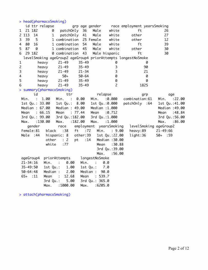
> head(pharmacoSmoking) id ttr relapse grp age gender race employment yearsSmoking1 21 182 0 patchOnly 36 Male white ft 262 113 14 1 patchOnly 41 Male white other 273 39 5 1 combination 25 Female white other 124 80 16 1 combination 54 Male white ft 395 87 0 1 combination 45 Male white other 306 29 182 0 combination 43 Male hispanic ft 30 levelSmoking ageGroup2 ageGroup4 priorAttempts longestNoSmoke1 heavy 21-49 35-49 0 02 heavy 21-49 35-49 3 903 heavy 21-49 21-34 3 214 heavy 50+ 50-64 0 05 heavy 21-49 35-49 0 06 heavy 21-49 35-49 2 1825> summary(pharmacoSmoking) id ttr relapse grp age Min. : 1.00 Min. : 0.00 Min. :0.000 combination:61 Min. :22.00 1st Qu.: 33.00 1st Qu.: 8.00 1st Qu.:0.000 patchOnly :64 1st Qu.:41.00 Median : 67.00 Median : 49.00 Median :1.000 Median :49.00 Mean : 66.15 Mean : 77.44 Mean :0.712 Mean :48.84 3rd Qu.: 99.00 3rd Qu.:182.00 3rd Qu.:1.000 3rd Qu.:56.00 Max. :130.00 Max. :182.00 Max. :1.000 Max. :86.00 gender race employment yearsSmoking levelSmoking ageGroup2 Female:81 black :38 ft :72 Min. : 9.00 heavy:89 21-49:66 Male :44 hispanic: 8 other:39 1st Qu.:22.00 light:36 50+ :59 other : 2 pt :14 Median :30.00 white :77 Mean :30.88 3rd Qu.:39.00 Max. :56.00 ageGroup4 priorAttempts longestNoSmoke 21-34:16 Min. : 0.00 Min. : 0.0 35-49:50 1st Qu.: 1.00 1st Qu.: 7.0 50-64:48 Median : 2.00 Median : 90.0 65+ :11 Mean : 12.68 Mean : 539.7 3rd Qu.: 5.00 3rd Qu.: 365.0 Max. :1000.00 Max. :6205.0

> attach(pharmacoSmoking)

of 12

> TimeToRelapse = Surv(ttr,relapse)> sort(TimeToRelapse) [1] 0 0 0 0 0 0 0 0 0 0 0 0 1 1 1 [16] 1 1 2 2 2 2 2 2 3 4 4 4 5 5 6 [31] 7 8 8 8 10 12 12 14 14 14 14 14 14 14 15 [46] 15 15 15 16 20 21 21 25 28 28 28 30 30 30 40 [61] 42 45 49 50 56 56 56 56 56 60 60 63 63 65 75 [76] 77 77 80 84 100 105 110 140 140 140 140 155 170 170 182+ [91] 182+ 182+ 182+ 182+ 182+ 182+ 182+ 182+ 182+ 182+ 182+ 182+ 182+ 182+ 182+[106] 182+ 182+ 182+ 182+ 182+ 182+ 182+ 182+ 182+ 182+ 182+ 182+ 182+ 182+ 182+[121] 182+ 182+ 182+ 182+ 182+

> # Fit a Weibull model with just treatment group, which was randomly assigned.> Model0 = survreg(TimeToRelapse~grp,dist='weibull')

Error in survreg(TimeToRelapse ~ grp, dist = "weibull") : Invalid survival times for this distribution

> # Error, likely choking on the zeros.> DayOfRelapse = Surv(ttr+1,relapse) # Day of relapse starts with one.> Model0 = survreg(DayOfRelapse~grp,dist='weibull') > summary(Model0)

Call:survreg(formula = DayOfRelapse ~ grp, dist = "weibull") Value Std. Error z p(Intercept) 5.260 0.3053 17.23 1.60e-66grppatchOnly -1.162 0.3999 -2.91 3.67e-03Log(scale) 0.606 0.0904 6.70 2.14e-11

Scale= 1.83

Weibull distributionLoglik(model)= -472.1 Loglik(intercept only)= -476.5

Chisq= 8.78 on 1 degrees of freedom, p= 0.003 Number of Newton-Raphson Iterations: 5 n= 125

Conclusion is that combination therapy is more effective. But the alphabetical order of

treatments makes combination the reference category, and this is clumsy. Make patch-

only the reference category and re-run. See analysis of the cars data for an example.

of 12

> contrasts(grp) = contr.treatment(2,base=2)> colnames(contrasts(grp)) = c('Combo') # Names of dummy vars -- just one> Model1 = survreg(DayOfRelapse~grp,dist='weibull') > summary(Model1)

Call:survreg(formula = DayOfRelapse ~ grp, dist = "weibull") Value Std. Error z p(Intercept) 4.098 0.2548 16.09 3.22e-58grpCombo 1.162 0.3999 2.91 3.67e-03Log(scale) 0.606 0.0904 6.70 2.14e-11

Scale= 1.83



> > betahat = Model1$coefficients; betahat(Intercept) grpCombo 4.097999 1.161901 > b0 = betahat[1]; b1 = betahat[2]> sigmahat = Model1$scale; sigmahat[1] 1.832392> Vhat = vcov(Model1); Vhat (Intercept) grpCombo Log(scale)(Intercept) 0.064903153 -0.065806535 -0.001649823grpCombo -0.065806535 0.159909904 0.006128624Log(scale) -0.001649823 0.006128624 0.008179519

> # Asymptotic covariance matrix comes out in terms of Log(scale), which is > # a minor pain. > > # 1) When patients receive the combination drug therapy rather than nicotine patch only, expected relapse time is multiplied by _______ .> # a) Give an estimate> # b) Modify the CI for beta1 to get a 95% confidence interval (don't use the delta method).> > # a) Give an estimate > exp(b1)grpCombo 3.196004 >

of 12

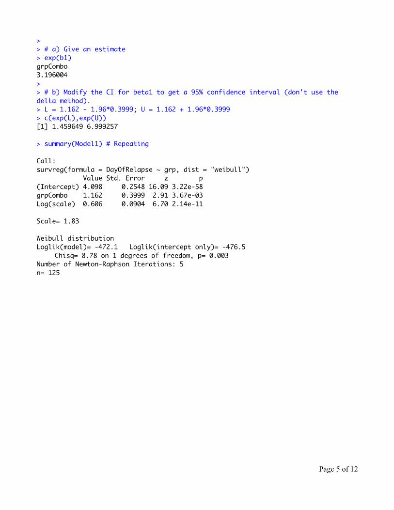
> > # a) Give an estimate > exp(b1)grpCombo 3.196004 > > # b) Modify the CI for beta1 to get a 95% confidence interval (don't use the delta method).> L = 1.162 - 1.96*0.3999; U = 1.162 + 1.96*0.3999> c(exp(L),exp(U))[1] 1.459649 6.999257

> summary(Model1) # Repeating

Call:survreg(formula = DayOfRelapse ~ grp, dist = "weibull") Value Std. Error z p(Intercept) 4.098 0.2548 16.09 3.22e-58grpCombo 1.162 0.3999 2.91 3.67e-03Log(scale) 0.606 0.0904 6.70 2.14e-11

Scale= 1.83



of 12

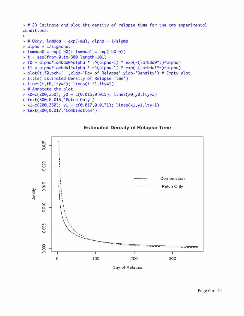
> # 2) Estimate and plot the density of relapse time for the two experimental conditions.> > # Okay, lambda = exp(-mu), alpha = 1/sigma> alpha = 1/sigmahat> lambda0 = exp(-b0); lambda1 = exp(-b0-b1) > t = seq(from=0,to=300,length=101)> f0 = alpha*lambda0âlpha * t^(alpha-1) * exp(-(lambda0*t)âlpha)> f1 = alpha*lambda1âlpha * t^(alpha-1) * exp(-(lambda1*t)âlpha)> plot(t,f0,pch=' ',xlab='Day of Relapse',ylab='Density') # Empty plot> title('Estimated Density of Relapse Time')> lines(t,f0,lty=2); lines(t,f1,lty=1)> # Annotate the plot> x0=c(200,250); y0 = c(0.015,0.015); lines(x0,y0,lty=2)> text(300,0.015,'Patch Only')> x1=c(200,250); y1 = c(0.017,0.0171); lines(x1,y1,lty=1)> text(300,0.017,'Combination')

of 12

> # 3) Estimate median time to relapse for the 2 groups, with CIs> # Asymptotic covariance matrix comes out in terms of Log(scale), which is > # unfortunate. > # Denote log(sigma) by s, and re-write g(theta) = exp(beta0) * log(2)^sigma > # as g(theta) = exp(beta0) * log(2)êxp(s) > shat = log(sigmahat)> > # Patch Only> medianhat0 = exp(b0)*log(2)^sigmahat> # gdot will be a 1 x 3 matrix.> gdot0 = cbind( exp(b0)*log(2)êxp(shat), 0, exp(b0) * log(2)êxp(shat) * log(log(2)) * exp(shat) ) > se0 = sqrt( as.numeric(gdot0 %*% Vhat %*% t(gdot0)) ); se0[1] 8.18674> lower0 = medianhat0 - 1.96*se0; upper0 = medianhat0 + 1.96*se0> patchonly = c(medianhat0,lower0,upper0)> names(patchonly) = c('Median','Lower95','Upper95')> patchonly Median Lower95 Upper95 30.76581 14.71980 46.81182 > > # Combination drug treatment> medianhat1 = exp(b0+b1)*log(2)^sigmahat> gdot1 = cbind( exp(b0+b1)*log(2)êxp(shat), exp(b0+b1)*log(2)êxp(shat), + exp(b0+b1) * log(2)êxp(shat) * log(log(2)) * exp(shat) ) > se1 = sqrt( as.numeric(gdot1 %*% Vhat %*% t(gdot1)) ); se1[1] 29.64109> lower1 = medianhat1 - 1.96*se1; upper1 = medianhat1 + 1.96*se1> combination = c(medianhat1,lower1,upper1)> names(combination) = c('Median','Lower95','Upper95')> combination Median Lower95 Upper95 98.32767 40.23114 156.42420 > > # There is an easier way to get these numbers> # help(predict.survreg)> Justpatch = data.frame(grp='patchOnly') > # A data frame with just one case and one variable.> Combination = data.frame(grp='combination')> treatments = rbind(Justpatch,Combination); treatments grp1 patchOnly2 combination

of 12

> # The 0.5 quantile is the median> medians = predict(Model1,newdata=treatments,type='quantile',p=0.5,se=TRUE)> medians$fit 1 2 30.76581 98.32767

$se.fit 1 2 8.18674 29.64109

> cbind(medians$fit,medians$se) [,1] [,2]1 30.76581 8.186742 98.32767 29.64109> rbind(c(medianhat0,se0),+ c(medianhat1,se1) ) (Intercept) [1,] 30.76581 8.18674[2,] 98.32767 29.64109> > # 4) Give a confidence interval for the difference between medians> > diffmed = medianhat1 - medianhat0> sed = sqrt(se0^2 + se1^2)> lowerd = diffmed - 1.96*sed; upperd = diffmed + 1.96*sed> differ = c(diffmed,lowerd,upperd)> names(differ) = c('Difference','Lower95','Upper95')> differDifference Lower95 Upper95 67.56186 7.29013 127.83359 >

of 12

> # 5) Plot the Kaplan-Meier estimates and MLEs of S(t)> > KM = survfit(DayOfRelapse~grp, type="kaplan-meier") # Kaplan-Meier is the default> summary(KM)Call: survfit(formula = DayOfRelapse ~ grp, type = "kaplan-meier")

grp=combination time n.risk n.event survival std.err lower 95% CI upper 95% CI 1 61 4 0.934 0.0317 0.874 0.999 3 57 3 0.885 0.0408 0.809 0.969 5 54 1 0.869 0.0432 0.788 0.958 6 53 2 0.836 0.0474 0.748 0.934 9 51 2 0.803 0.0509 0.709 0.909 11 49 1 0.787 0.0524 0.691 0.897 13 48 1 0.770 0.0538 0.672 0.884 15 47 1 0.754 0.0551 0.653 0.870 16 46 2 0.721 0.0574 0.617 0.843 17 44 1 0.705 0.0584 0.599 0.829 21 43 1 0.689 0.0593 0.582 0.815 22 42 1 0.672 0.0601 0.564 0.801 31 41 2 0.639 0.0615 0.530 0.772 43 39 1 0.623 0.0621 0.512 0.757 51 38 1 0.607 0.0625 0.496 0.742 57 37 2 0.574 0.0633 0.462 0.712 61 35 2 0.541 0.0638 0.429 0.682 64 33 2 0.508 0.0640 0.397 0.650 66 31 1 0.492 0.0640 0.381 0.635 76 30 1 0.475 0.0639 0.365 0.619 111 29 1 0.459 0.0638 0.350 0.603 141 28 3 0.410 0.0630 0.303 0.554 171 25 1 0.393 0.0625 0.288 0.537

grp=patchOnly time n.risk n.event survival std.err lower 95% CI upper 95% CI 1 64 8 0.875 0.0413 0.798 0.960 2 56 5 0.797 0.0503 0.704 0.902 3 51 3 0.750 0.0541 0.651 0.864 4 48 1 0.734 0.0552 0.634 0.851 5 47 2 0.703 0.0571 0.600 0.824 7 45 1 0.688 0.0579 0.583 0.811 8 44 1 0.672 0.0587 0.566 0.797 9 43 1 0.656 0.0594 0.550 0.784 13 42 1 0.641 0.0600 0.533 0.770 15 41 6 0.547 0.0622 0.438 0.684 16 35 2 0.516 0.0625 0.407 0.654 22 33 1 0.500 0.0625 0.391 0.639 26 32 1 0.484 0.0625 0.376 0.624

of 12

29 31 3 0.437 0.0620 0.331 0.578 31 28 1 0.422 0.0617 0.317 0.562 41 27 1 0.406 0.0614 0.302 0.546 46 26 1 0.391 0.0610 0.288 0.530 50 25 1 0.375 0.0605 0.273 0.515 57 24 3 0.328 0.0587 0.231 0.466 78 21 2 0.297 0.0571 0.204 0.433 81 19 1 0.281 0.0562 0.190 0.416 85 18 1 0.266 0.0552 0.177 0.399 101 17 1 0.250 0.0541 0.164 0.382 106 16 1 0.234 0.0530 0.151 0.365 141 15 1 0.219 0.0517 0.138 0.348 156 14 1 0.203 0.0503 0.125 0.330 171 13 1 0.187 0.0488 0.113 0.312

> # Look at K-M estimates of medians> KM[1] # CombinationCall: survfit(formula = DayOfRelapse ~ grp, type = "kaplan-meier")

n events median 0.95LCL 0.95UCL 61 37 66 51 NA > KM[2] # Patch OnlyCall: survfit(formula = DayOfRelapse ~ grp, type = "kaplan-meier")

n events median 0.95LCL 0.95UCL 64 52 24 15 57

> # Repeat MLEs for comparison> combination Median Lower95 Upper95 98.32767 40.23114 156.42420 > patchonly Median Lower95 Upper95 30.76581 14.71980 46.81182

of 12

> plot(KM, xlab='t', ylab='Survival Probability', lwd=2, col=1:2) > # 1 is black, 2 is red> legend(x=125,y=1.0, col=1:2, lwd=2, legend=c('Combination','Patch Only'))> title(expression(paste(hat(S)(t),': Kaplan-Meier and Maximum Likelihood Estimates')))> # MLEs> x = 1:185> lambda0 = exp(-b0); lambda1 = exp(-b0-b1); alpha=1/sigmahat> Shat0 = exp(-(lambda0*x)^alpha); Shat1 = exp(-(lambda1*x)^alpha)> lines(x,Shat0,lty=2,col=2) # Patch only is red> lines(x,Shat1,lty=2) # Combination is black (default)

of 12

> > # Non-parametric rank test of equal survival functions> # See http://dwoll.de/rexrepos/posts/survivalKM.html> survdiff(DayOfRelapse~grp)Call:survdiff(formula = DayOfRelapse ~ grp)

N Observed Expected (O-E)^2/E (O-E)^2/Vgrp=combination 61 37 49.9 3.36 8.03grp=patchOnly 64 52 39.1 4.29 8.03

Chisq= 8 on 1 degrees of freedom, p= 0.00461

> # Compare p = 0.00367 from Z-test of H0: beta1=0> >

This document was prepared by Jerry Brunner, University of Toronto. It is licensed under a Creative Commons Attribution - ShareAlike 3.0 Unported License: http://creativecommons.org/licenses/by-sa/3.0/deed.en_US. Use any part of it as you like and share the result freely. It is available in OpenOffice.org format from the course website:

http://www.utstat.toronto.edu/~brunner/oldclass/312s19

of 12

weibull regression with r, part onebrunner/oldclass/312s19/...> # 3) estimate median time to...

Documents