HAL Id: hal-01652194https://hal.archives-ouvertes.fr/hal-01652194

Submitted on 30 Nov 2017

HAL is a multi-disciplinary open accessarchive for the deposit and dissemination of sci-entific research documents, whether they are pub-lished or not. The documents may come fromteaching and research institutions in France orabroad, or from public or private research centers.

L’archive ouverte pluridisciplinaire HAL, estdestinée au dépôt et à la diffusion de documentsscientifiques de niveau recherche, publiés ou non,émanant des établissements d’enseignement et derecherche français ou étrangers, des laboratoirespublics ou privés.

Weighted-feature and cost-sensitive regression model forcomponent continuous degradation assessment

Jie Liu, Enrico Zio

To cite this version:Jie Liu, Enrico Zio. Weighted-feature and cost-sensitive regression model for component continuousdegradation assessment. Reliability Engineering and System Safety, Elsevier, 2017, 168, pp.210 - 217.<10.1016/j.ress.2017.03.012>. <hal-01652194>

Reliability Engineering and System Safety 168 (2017) 210–217

Contents lists available at ScienceDirect

Reliability Engineering and System Safety

journal homepage: www.elsevier.com/locate/ress

Weighted-feature and cost-sensitive regression model for component continuous degradation assessment

Jie Liu

a , Enrico Zio

a , b , ∗

a Chair on System Science and the Energetic Challenge, EDF Foundation, Laboratoire Genie Industriel, CentraleSupélec, Université Paris-Saclay, Grande voie des Vignes,

92290 Chatenay-Malabry, France b Energy Department, Politecnico di Milano, Milano, Italy

a r t i c l e i n f o

Keywords:

Condition-based maintenance Cost-sensitive Continuous degradation assessment Feature vector regression Feature vector selection Weighted-feature

a b s t r a c t

Conventional data-driven models for component degradation assessment try to minimize the average estimation accuracy on the entire available dataset. However, an imbalance may exist among different degradation states, because of the specific data size and/or the interest of the practitioners on the different degradation states. Specifically, reliable equipment may experience long periods in low-level degradation states and small times in high-level ones. Then, the conventional trained models may result in overfitting the low-level degradation states, as their data sizes overwhelm the high-level degradation states. In practice, it is usually more interesting to have accurate results on the high-level degradation states, as they are closer to the equipment failure. Thus, during the training of a data-driven model, larger error costs should be assigned to data points with high-level degradation states when the training objective minimizes the total costs on the training dataset. In this paper, an efficient method is proposed for calculating the costs for continuous degradation data. Considering the different influence of the features on the output, a weighted-feature strategy is integrated for the development of the data-driven model. Real data of leakage of a reactor coolant pump is used to illustrate the application and effectiveness of the proposed approach.

© 2017 Elsevier Ltd. All rights reserved.

1

c

m

p

o

C

v

r

d

t

n

c

[

f

p

T

d

d

d

l

a

d

t

u

s

a

m

s

d

a

o

d

f

s

e

hA0

. Introduction

Condition-Based Maintenance (CBM) has gained much attention re-ently [23,32,8] . Advanced sensors implemented in production systemseasure physical variables related to the equipment degradation androper maintenance is recommended based on the assessed degradationf the equipment. Compared to corrective and scheduled maintenance,BM can reduce the direct and indirect costs of maintenance and pre-ent catastrophic failure [1] .

One of the cornerstones of CBM is the precise assessment of the cur-ent degradation state of the equipment of interest. If it is monitoredirectly by sensors, it is relatively easy to identify the system degrada-ion state. Otherwise, the degradation state of the equipment of interesteeds to be informed from the related monitored variables. For the latterase, physical [13,25] , knowledge-based [12,26] or data-driven models16,33] can be integrated depending on the available knowledge, in-ormation and data on the degradation [36,46] . Data-driven models, inarticular, benefit from high computation speed and advanced sensors.hese models can be classified also based on the type of the underlying

∗ Corresponding author at: Chair on System Science and the Energetic Challenge, EDF Foundes Vignes, 92290 Chatenay-Malabry, France.

E-mail address: enrico.zio@polimi.it (E. Zio).

d

ttp://dx.doi.org/10.1016/j.ress.2017.03.012 vailable online 22 March 2017 951-8320/© 2017 Elsevier Ltd. All rights reserved.

egradation process, i.e. proportional hazard models [30] , discrete-stateegradation [24] , continuous-state degradation [1] .

In this work, we focus on the data-driven models with supervisedearning methods for continuous degradation assessment. Assuming that pool of degradation patterns of similar equipment are available, a data-riven model is trained off-line with the recorded degradation data and,hen, it is used to assess on-line the degradation state of an equipmentnder operation. Shen et al. [34] adopt a fuzzy support vector data de-cription to construct a fuzzy-monitoring coefficient, which serves as monotonic damage index of bearing degradation. Logistic regressionodels and incremental rough support vector data description are used

eparately in Caesarendra et al. [6] and Zhu et al. [45] for bearing degra-ation assessment. Principal component analysis is used in Gómez etl. [10] to obtain soil degradation indexes for distinguishing betweenlive farms with low soil degradation and those in a serious state ofegradation. Peng et al. [28] use an inverse Gaussian process modelor degradation modelling. Nonhomogeneous continuous-time hiddenemi-Markov process is proposed in Moghaddass and Zuo [24] for mod-lling the degradation of devices undergoing discrete, multistate degra-ation. Vale and Lurdes [37] employ a stochastic model for character-

ation, Laboratoire Genie Industriel, CentraleSupélec, Université Paris-Saclay, Grande voie

J. Liu, E. Zio Reliability Engineering and System Safety 168 (2017) 210–217

i

N

s

t

i

i

t

F

d

t

d

o

p

f

d

a

t

s

w

t

e

r

d

u

f

d

j

t

s

e

T

f

p

T

d

d

m

a

t

i

[

s

o

e

r

p

i

c

n

i

O

c

p

T

t

t

t

c

m

t

s

t

m

n

m

t

o

s

c

p

w

a

a

f

s

v

H

e

m

fl

h

a

t

t

t

w

F

c

R

t

i

T

t

i

b

f

a

s

m

t

p

c

b

s

l

S

2

a

e

F

f

e

v

i

o

a

p

t

d

p

f

zing the track geometry degradation process in the Portuguese railwayorthern Line.

For the development of the previous data-driven models, it is as-umed that the pool of available degradation data is large and represen-ative of the different degradation states of the equipment. However,n practical cases, especially for highly reliable equipment, a problem ofmbalance often exists between different degradation states with respecto the knowledge, information and data available to characterize them.or highly reliable equipment, typically there is a long period withoutegradation or with low-level degradation states, and the data represen-ative of high-level degradation states are relatively limited. Training aata-driven model on the entire set of recorded data with the objectivef minimizing the average estimation error on the whole degradationrocess may lead to a relatively worse performance of the trained modelor the data of high level degradation states, as the data on the low-levelegradation states outnumber those on the high-level degradation statesnd the trained model overfits on the low-level degradation states. Onhe other hand, if the data on the high-level degradation states is notufficiently large and representative, training a data-driven model onlyith the data of high-level degradation states may lead to overfitting

he recorded data and low generalizability on test data. Furthermore,ven if the data on different degradation states are comparable and rep-esentative, the industrial practitioner may be more interested in someegradation states, e.g. the high-level degradation states, the peak val-es during the degradation process, as they are more critical for theunctioning of the equipment and, thus, require more accuracy. So, theata-driven model should be trained on the whole dataset, but the ob-ective can not be that of minimizing the average estimation error onhe whole dataset. In this work, an approach is proposed based on cost-ensitive regression models in combination of a weighted-feature strat-gy for the imbalance problem in continuous degradation assessment.o the authors ’ knowledge, no work has been reported on this problemor continuous degradation assessment.

Cost-sensitive models are very popular for solving classificationroblems with different costs for different misclassification errors [9] .hey have been successfully applied in medical diagnosis [39] , objectetection [5] , intrusion detection [15] , face recognition [42] , softwareefect prediction [17] etc. The objective of training a cost-sensitiveodel is to minimize the total cost on the misclassification error in way to assign a larger cost to the error on the minority class thanhat on the majority class. Cost-sensitive models have been integratedn neural networks [14] , decision trees [41] , support vector machines38] , Bayesian networks [11] , etc. Different methods can be used to as-ign the costs for different misclassification errors and the most popularne is to set the costs based on expertise on the problem [40] . Differ-nt cost-assignment methods can be proposed considering the specificequirements and characteristics of the application. In the mentionedrevious works, discrete costs are assigned to different classes, assum-ng that the cost of the misclassification errors on the data of the samelass is the same. This is reasonable for classification problems with fi-ite classes. On the contrary, for regression of continuous degradation,t is infeasible to assign discrete costs for infinite degradation states.ne way is to discretize the continuous degradation states, but this mayause loss of information on the degradation states. This work tries toropose a method for assigning continuous costs to degradation states.he proposed method assigns larger costs to the regression errors onhe high-level degradation states than those to the low-level degrada-ion states and also larger costs to peak values than to normal values inheir neighborhoods.

The basic data-driven model used in this paper for integrating theost-sensitive strategy is Feature Vector Regression (FVR), a kernelethod proposed in Liu and Zio [20] . Training a FVR model requires fea-

ure vector selection and regression model construction. Feature vectorelection proceeds by selecting part of the training data points as fea-ure vectors in the Reproducing Kernel Hilbert Space (RKHS), where theapping of all training data points can be expressed as a linear combi-

211

ation of the selected feature vectors. Different to the traditional kernelethods that define the estimation function as a kernel expansion on all

he training dataset, the estimate function of FVR is a kernel expansionnly on the feature vectors. The objective is to minimize the regres-ion error on the whole training dataset. The parameters in FVR can bealculated analytically, without using a sophisticated method for tuningarameters in the model. FVR model is combined with cost-sensitive andeighted-feature strategies in this work. These strategies are not suit-ble only for FVR, but also for other regression models for degradationssessment.

Another original contribution of this work is the adopted weighted-eature strategy. Conventionally, after the raw data are pre-processed,ome features are selected as inputs and they form directly the inputectors which are used for training a supervised data-driven model.owever, the selected features may still have different levels of influ-nce on the output. In order to characterize this difference in kernelethods, larger weights are assigned to the features with a higher in-uence on the output in the kernel function. Weighted-feature strategyas been used in Amutha and Kavitha [3] , Peng et al. [29] , Phan etl. [31] , Liu et al. [18] . The weighted-feature strategy is integrated forhe first time with the basic model (FVR) in this work and it is alsohe first time that the weighted-feature strategy is used for degrada-ion assessment. An efficient optimization process is adopted in thisork for finding the weights for different features and the parameters inVR.

To demonstrate the proposed approach, we make use of a case studyoncerning the estimation of leakage of coolant water from the seal of aeactor Coolant Pump (RCP) in a Nuclear Power Plant (NPP). The con-

rol of the leakage is very important for safety reasons [21] . Sensors arenstalled to monitor the temperature, pressure, flow of coolant water.hese variables are informative for assessing the leakage amount. Whenhe amount of leakage is low, the reactor can make up the leakage by us-ng auxiliary and protection systems. But when it is large, the NPP muste shut down. Thus, operators are more concerned of correctly identi-ying the leakages of large magnitude than small. Correspondingly, theccuracy is more important in case of large amount of leakage than ofmall amount. However, as the NPP components are highly reliable,ost of the historical recorded data relates to low amounts of leakage,

he data on large amounts of leakage being far less. In this work, the pro-osed weighted-feature and cost-sensitive FVR is adopted for estimatingontinuously the leakage from the RCP.

The remainder of the paper is structured as follows. Section 2 recallsriefly the FVR method and introduces the approach proposed for as-essing continuous degradation with imbalance. The case study on theeakage from RCP is presented in Section 3 with experimental results.ome conclusions and perspectives are drawn in Section 4 .

. Weighted-feature and cost-sensitive FVR for degradation

ssessment

FVR proposed in Liu and Zio [20] is a kernel method, which allowsasy tuning of hyperparameters and offers a geometrical interpretation.VR reduces the size of the estimate function by selecting a number ofeature vectors and keeps its generalization power by minimizing therror on the whole training dataset. In this Section, FVR is briefly re-iewed firstly and, then, the weighted-feature and cost-sensitive FVR isntroduced, with details on the calculation of the costs and the tuningf the weight of each feature.

In the paper, ( 𝒙 , 𝑦 ) represents the input and corresponding output of nonlinear relation. 𝑘 ( 𝒙 1 , 𝒙 2 ) is the kernel function, taken as the innerroduct of 𝜑 ( 𝒙 1 ) and 𝜑 ( 𝒙 2 ) , i.e. ⟨𝜑 ( 𝒙 1 ) , 𝜑 ( 𝒙 2 ) ⟩, and 𝜑 ( 𝒙 ) is the functionhat maps the original data into a high dimensional space (i.e. Repro-ucing Kernel Hilbert Space (RKHS)), where the relation between in-ut and output becomes linear. The training dataset is 𝐓 = { ( 𝒙 𝑖 , 𝑦 𝑖 ) } ,or 𝑖 = 1 , 2 , … , 𝑁 . Without restricting the generalizability of the model,

J. Liu, E. Zio Reliability Engineering and System Safety 168 (2017) 210–217

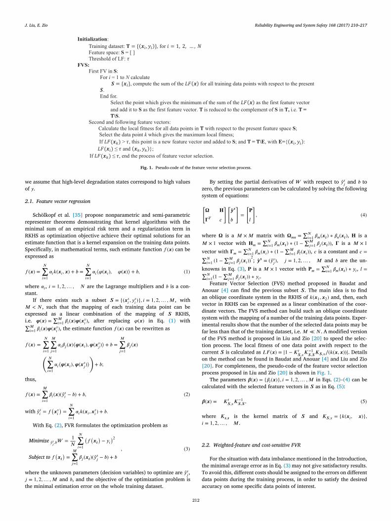
Fig. 1. Pseudo-code of the feature vector selection process.

w

o

2

r

m

R

e

S

e

𝑓

w

s

𝑀

e

i ∑𝑓

t

𝑓

w

w

𝑗

t

z

s[

w

𝑀

v ∑

k ∑

A

a

v

d

s

i

f

o

t

c

o

[

p

c

𝜷

w

𝑖

2

t

T

d

a

e assume that high-level degradation states correspond to high valuesf 𝑦 .

.1. Feature vector regression

Schölkopf et al. [35] propose nonparametric and semi-parametricepresenter theorems demonstrating that kernel algorithms with theinimal sum of an empirical risk term and a regularization term inKHS as optimization objective achieve their optimal solutions for anstimate function that is a kernel expansion on the training data points.pecifically, in mathematical terms, such estimate function 𝑓 ( 𝒙 ) can bexpressed as

( 𝒙 ) =

𝑁 ∑𝑖 =1

𝛼𝑖 𝑘 ( 𝒙 𝑖 , 𝒙 ) + 𝑏 =

𝑁 ∑𝑖 =1

𝛼𝑖 ⟨𝜑 ( 𝒙 𝑖 ) , 𝜑 ( 𝒙 ) ⟩ + 𝑏, (1)

here 𝛼𝑖 , 𝑖 = 1 , 2 , … , 𝑁 are the Lagrange multipliers and 𝑏 is a con-tant.

If there exists such a subset 𝑺 = {( 𝒙 𝑠 𝑖 , 𝑦 𝑠

𝑖 )} , 𝑖 = 1 , 2 , … , 𝑀 , with

< 𝑁 , such that the mapping of each training data point can bexpressed as a linear combination of the mapping of 𝑺 RKHS,.e. 𝝋 ( 𝒙 ) =

∑𝑀

𝑖 =1 𝛽𝑖 ( 𝒙 ) 𝝋 ( 𝒙 𝑠 𝑖 ) , after replacing 𝜑 ( 𝒙 ) in Eq. (1) with

𝑀

𝑖 =1 𝛽𝑖 ( 𝒙 ) 𝝋 ( 𝒙 𝑠 𝑖 ) , the estimate function 𝑓 ( 𝒙 ) can be rewritten as

( 𝒙 ) =

𝑁 ∑𝑖 =1

𝑀 ∑𝑗=1

𝛼𝑖 𝛽𝑗 ( 𝒙 ) ⟨𝝋 ( 𝒙 𝑖 ) , 𝝋 ( 𝒙 𝑠 𝑗 ) ⟩ + 𝑏 =

𝑀 ∑𝑗=1

𝛽𝑗 ( 𝒙 ) (

𝑁 ∑𝑖 =1

𝛼𝑖 ⟨𝝋 ( 𝒙 𝑖 ) , 𝝋 ( 𝒙 𝑠 𝑗 ) ⟩)

+ 𝑏 ;

hus,

( 𝒙 ) =

𝑀 ∑𝑖 =1

𝛽𝑖 ( 𝒙 )( ̂𝑦 𝑠 𝑖 − 𝑏 ) + 𝑏, (2)

ith �̂� 𝑠 𝑖 = 𝑓

(𝒙 𝑠 𝑖

)=

𝑁 ∑𝑖 =1

𝛼𝑖 𝑘 ( 𝒙 𝑖 , 𝒙 𝑠 𝑖 ) + 𝑏.

With Eq. (2) , FVR formulates the optimization problem as

Minimize �̂� 𝑠 𝑗 ,𝑏 𝑊 =

1 𝑁

𝑁 ∑𝑖 =1

(𝑓 (𝒙 𝒊 )− 𝑦 𝑖

)2 Subject to 𝑓

(𝒙 𝒊 )=

𝑀 ∑𝑗=1

𝛽𝑗 ( 𝒙 𝒊 )( ̂𝑦 𝑠 𝑗 − 𝑏 ) + 𝑏

, (3)

here the unknown parameters (decision variables) to optimize are �̂� 𝑠 𝑗 ,

= 1 , 2 , … , 𝑀 and 𝑏 , and the objective of the optimization problem ishe minimal estimation error on the whole training dataset.

212

By setting the partial derivatives of 𝑊 with respect to �̂� 𝑠 𝑗

and 𝑏 toero, the previous parameters can be calculated by solving the followingystem of equations:

𝛀 𝐇

𝚪𝑇 𝑐

] [

�̂� 𝒔

𝑏

]

=

[

𝐏

𝑙

]

, (4)

here 𝛀 is a 𝑀 ×𝑀 matrix with 𝛀𝑚𝑛 =

∑𝑁

𝑖 =1 𝛽𝑚 ( 𝒙 𝒊 ) ∗ 𝛽𝑛 ( 𝒙 𝒊 ) , 𝐇 is a

× 1 vector with 𝐇 𝑚 =

∑𝑁

𝑖 =1 𝛽𝑚 ( 𝒙 𝒊 ) ∗ (1 −

∑𝑀

𝑗=1 𝛽𝑗 ( 𝒙 𝒊 )) , 𝚪 is a 𝑀 × 1ector with 𝚪𝑚 =

∑𝑁

𝑖 =1 𝛽𝑚 ( 𝒙 𝑖 ) ∗ (1 −

∑𝑀

𝑙=1 𝛽𝑙 ( 𝒙 𝑖 )) , 𝑐 is a constant and 𝑐 =𝑁

𝑖 =1 (1 −

∑𝑀

𝑗=1 𝛽𝑗 ( 𝒙 𝑖 )) 2 ; �̂� 𝒔 = ( ̂𝑦 𝑠

𝑗 ) , 𝑗 = 1 , 2 , … , 𝑀 and 𝑏 are the un-

nowns in Eq. (3) , 𝐏 is a 𝑀 × 1 vector with 𝐏 𝑚 =

∑𝑁

𝑖 =1 𝛽𝑚 ( 𝒙 𝒊 ) ∗ 𝑦 𝑖 , 𝑙 =𝑁

𝑖 =1 (1 −

∑𝑀

𝑗=1 𝛽𝑗 ( 𝒙 𝑖 )) ∗ 𝑦 𝑖 . Feature Vector Selection (FVS) method proposed in Baudat and

nouar [4] can find the previous subset 𝑺 . The main idea is to findn oblique coordinate system in the RKHS of 𝑘 ( 𝒙 1 , 𝒙 2 ) and, then, eachector in RKHS can be expressed as a linear combination of the coor-inate vectors. The FVS method can build such an oblique coordinateystem with the mapping of a number of the training data points. Exper-mental results show that the number of the selected data points may bear less than that of the training dataset, i.e. 𝑀 ≪ 𝑁 . A modified versionf the FVS method is proposed in Liu and Zio [20] to speed the selec-ion process. The local fitness of one data point 𝒙 with respect to theurrent 𝑺 is calculated as 𝐿𝐹 ( 𝒙 ) = |1 − 𝐾

𝑡 𝑺 ,𝑥

𝐾

−1 𝑺 , 𝑺

𝐾 𝑺 ,𝑥 ∕( 𝑘 ( 𝒙 , 𝒙 )) |. Detailsn the method can be found in Baudat and Anouar [4] and Liu and Zio20] . For completeness, the pseudo-code of the feature vector selectionrocess proposed in Liu and Zio [20] is shown in Fig. 1 .

The parameters 𝜷( 𝒙 ) = { 𝛽𝑖 ( 𝒙 )} , 𝑖 = 1 , 2 , … , 𝑀 in Eqs. (2)–(4) can bealculated with the selected feature vectors in 𝑺 as in Eq. (5) :

( 𝒙 ) = 𝐾

𝑡 𝑺 ,𝑥

𝐾

−1 𝑺 , 𝑺

, (5)

here 𝐾 𝒔 , 𝒔 is the kernel matrix of 𝑺 and 𝐾 𝑺 ,𝑥 = { 𝑘 ( 𝒙 𝑖 , 𝒙 )} , = 1 , 2 , … , 𝑀 .

.2. Weighted-feature and cost-sensitive FVR

For the situation with data imbalance mentioned in the Introduction,he minimal average error as in Eq. (3) may not give satisfactory results.o avoid this, different costs should be assigned to the errors on differentata points during the training process, in order to satisfy the desiredccuracy on some specific data points of interest.

J. Liu, E. Zio Reliability Engineering and System Safety 168 (2017) 210–217

p

w

d

f

v

o

o

c[

w

𝑀

v ∑

𝑦

k

𝑪

r

f

v

h

s

i

v

a

w

𝑐

w

E

(

𝑎

𝑠

𝑑

u

h

v

p

a

t

t

f

f

k

t

u

r

m

c

w

a

w

c

3

k

l

M

e

e

w

r

𝛾

t

p

4

w

𝜔

t

s

o

v

t

3

t

a

g

t

s

w

F

(

(

o

a

w

i

w

t

Another issue regards the usefulness of different features for the out-ut assessment: the features need to be treated differently and largereights should be assigned to the more useful ones. In kernel methods,ifferent weights can be assigned to different features by using kernelunction 𝑘 ( 𝝎 . ∗ 𝒙 1 , 𝝎 . ∗ 𝒙 2 ) instead of 𝑘 ( 𝒙 1 , 𝒙 2 ) , where 𝝎 is the weightector (of the same size as 𝒙 ) of the usefulness of each feature andperator. ∗ is the element-wise multiplication.

Initiating the costs of different data points as 𝑪 = [ 𝑐 1 , 𝑐 2 , … , 𝑐 𝑁

] , theptimization problem in Eq. (3) can be reformulated as

Minimize �̂� 𝑠 𝑗 ,𝑏 𝑊 =

1 𝑁

𝑁 ∑𝑖 =1

𝑐 𝑖 (𝑓 (𝒙 𝒊 )− 𝑦 𝑖

)2 Subject to 𝑓

(𝒙 𝒊 )=

𝑀 ∑𝑗=1

𝛽𝑗 ( 𝒙 𝒊 )( ̂𝑦 𝑠 𝑗 − 𝑏 ) + 𝑏

. (6)

The unknown parameters �̂� 𝑠 𝑗 , 𝑗 = 1 , 2 , … , 𝑀 and 𝑏 in Eq. (6) can be

alculated by solving the following equation:

𝛀 𝐇

𝚪𝑇 𝑐

] [

�̂� 𝒔

𝑏

]

=

[

𝐏

𝑙

]

, (7)

here 𝛀 is a 𝑀 ×𝑀 matrix with 𝛀𝑚𝑛 =

∑𝑁

𝑖 =1 𝑐 𝑖 𝛽𝑚 ( 𝒙 𝒊 ) ∗ 𝛽𝑛 ( 𝒙 𝒊 ) , 𝐇 is a

× 1 vector with 𝐇 𝑚 =

∑𝑁

𝑖 =1 𝑐 𝑖 𝛽𝑚 ( 𝒙 𝒊 ) ∗ (1 −

∑𝑀

𝑗=1 𝛽𝑗 ( 𝒙 𝒊 )) , 𝚪 is a 𝑀 × 1ector with 𝚪𝑚 =

∑𝑁

𝑖 =1 𝑐 𝑖 𝛽𝑚 ( 𝒙 𝑖 ) ∗ (1 −

∑𝑀

𝑙=1 𝛽𝑙 ( 𝒙 𝑖 )) , 𝑐 is a constant and 𝑐 =𝑁

𝑖 =1 𝑐 𝑖 (1 −

∑𝑀

𝑗=1 𝛽𝑗 ( 𝒙 𝑖 )) 2 ; 𝐏 is a 𝑀 × 1 vector with 𝐏 𝑚 =

∑𝑁

𝑖 =1 𝑐 𝑖 𝛽𝑚 ( 𝒙 𝒊 ) ∗ 𝑖 , 𝑙 =

∑𝑁

𝑖 =1 𝑐 𝑖 (1 −

∑𝑀

𝑗=1 𝛽𝑗 ( 𝒙 𝑖 )) ∗ 𝑦 𝑖 . The parameters 𝜷( 𝒙 ) are still calculated with Eq. (5) , but with the

ernel function 𝑘 ( 𝝎 . ∗ 𝒙 1 , 𝝎 . ∗ 𝒙 2 ) . In this model, the unknown parameters include the cost vector

= [ 𝑐 1 , 𝑐 2 , … , 𝑐 𝑁

] , the weight vector 𝝎 = [ 𝜔 1 , 𝜔 2 , … , 𝜔 𝑁

] and the pa-ameters related to the kernel function.

The cost vector 𝑪 can be calculated analytically. In this work, weocus on the peak values and high-level degradation states. The peakalues may occur abruptly and cause the failures of the system. Theigh-level degradation states are reached close to the failure state of theystem and, thus, it is even more important to get good accuracy. Thus,n this work, the cost is dependent on the degradation state and peakalue. A large cost is, thus, assigned to data points which are peak valuesnd high-level degradation states. Specifically, for a data point ( 𝒙 𝑡 , 𝑦 𝑡 )ith 𝑡 = 1 , 2 , … , 𝑁 , its cost is calculated as

𝑡 = 𝑒 ( 𝑠 𝑡 + 𝑑 𝑡 )∕ 𝜎, (8)

here 𝑠 𝑡 is the score of the point with respect to the peak function inq. (9) [27] and 𝑑 𝑡 is the normalized degradation value of 𝑦 𝑡 as in Eq.10) :

𝑡 =

⎧ ⎪ ⎪ ⎨ ⎪ ⎪ ⎩ 𝑦 𝑡 −

1 2 𝑘

∑2 𝑘 +1 𝑖 =1 ; 𝑖 ≠𝑡 𝑦 𝑖 , if 𝑡 ≤ 𝑘

𝑦 𝑡 −

1 2 𝑘

∑𝑡 + 𝑘 𝑖 = 𝑡 − 𝑘 ; 𝑖 ≠𝑡 𝑦 𝑖 , if 𝑘 < 𝑡 < 𝑁 − 𝑘

𝑦 𝑡 −

1 2 𝑘

∑𝑁

𝑖 = 𝑁−2 𝑘 ; 𝑖 ≠𝑡 𝑦 𝑖 , if 𝑡 ≥ 𝑁 − 𝑘

, f 𝑜𝑟 𝑡 = 1 , 2 , … , 𝑁 ,

𝑡 =

𝑎 𝑡 − min ( 𝒂 ) max ( 𝒂 ) − min ( 𝒂 )

∗ 0 . 8 + 0 . 1 , with 𝒂 = [ 𝑎 1 , 𝑎 2 , … , 𝑎 𝑁

] , (9)

𝑡 =

𝑦 𝑡 − min ( 𝒚 ) max ( 𝒚 ) − min ( 𝒚 )

∗ 0 . 8 + 0 . 1 , with 𝒚 = [ 𝑦 1 , 𝑦 2 , … , 𝑦 𝑁

] . (10)

The cost is composed of two parts: 𝑠 𝑡 and 𝑑 𝑡 . Peak degradation val-es have high scores 𝑠 𝑡 and high-level degradation states have relativelyigh values of 𝑑 𝑡 . The two values, 𝑠 𝑡 and 𝑑 𝑡 are normalized in the inter-al [0.1 0.9] to have equal weights on the cost of one data point. Thearameter 𝜎 in Eq. (8) is a case-specific value that must be set by thenalyst: the smaller the value of 𝜎 is, the larger the difference betweenhe different costs.

213

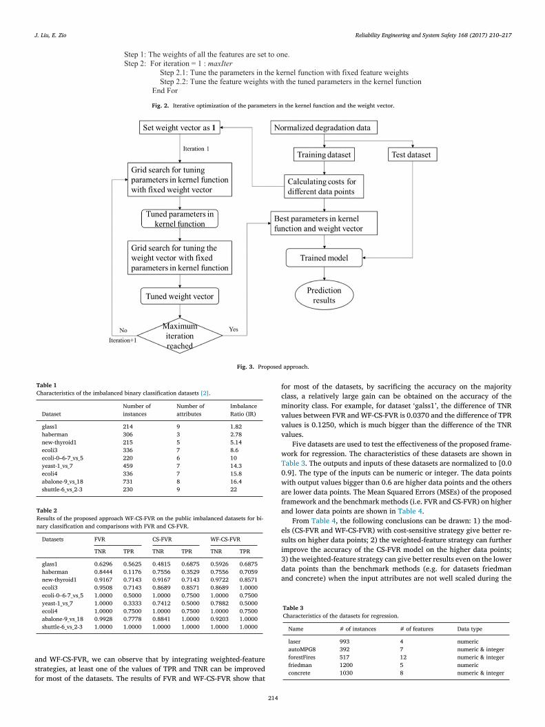
For the parameters in the kernel function and for the weight vec-or for the different features, an iterative procedure is proposed ( Fig. 2 )or minimizing the total cost in Eq. (6) . An initial weight vector for theeatures is set to 1 . With the fixed weight vector, the parameters in theernel function are tuned and, then, with the tuned parameters value inhe kernel function, the weight vector is tuned. The process is repeatedntil a fixed number of iterations maxIter is reached. For tuning the pa-ameters in the kernel function or the weight vector, conventional opti-ization methods, e.g. genetic algorithm [43] , grid search [19] , parti-

le swarm optimization [44] , ant colony optimization [22] can be used,ith the objective of minimizing the total cost on the training datasets in Eq. (6) . Note that during the optimization process, the sum of theeights for the features equals always that of the initial weights. The

onvergence of the iterative optimization process is shown in Section 3 .

. Case study

The implementation of the proposed approach is sketched in Fig. 3 .In the experiment, the Radial Basis kernel Function (RBF) is used as

ernel function, i.e. 𝑘 ( 𝒙 1 , 𝒙 2 ) = 𝑒

− ‖𝒙 1 − 𝒙 2 ‖2 2 𝛾2 . The value of 𝛾 can be calcu-

ated analytically with Eq. (11) below, as proposed by Cherkassky anda [7] , whereas the value for 𝜇 is chosen between 0 and 1: by trial and

rror, the value of 𝜇 is set to 0.2. Thus, no explicit optimization method,.g. grid search, is used for tuning the parameters in RBF. Given theeight vector 𝝎 , the value of 𝛾 is calculated directly with Eq. (11) after

eplacing 𝒙 by 𝝎 . ∗ 𝒙 .

2 = 𝜇 ∗ m 𝑎𝑥 ‖𝒙 𝑖 − 𝒙 𝑗 ‖2 , 𝑖, 𝑗 = 1 , … , 𝑁 (11)

With the calculated value of 𝛾, a grid search method is used to tunehe weights of the different features. Suppose there are 𝐾 features: theossible relative weight 𝑟 𝑖 of one feature can be drawn from R = [1 2 3 5 6 7 8 9] with equal probability; for each combination of the relativeeights [ 𝑟 1 , 𝑟 2 , … , 𝑟 𝐾 ], the weight vector 𝝎 is calculated as

𝑖 = 𝑁 𝑓 ∗ 𝑟 𝑖 / 𝐾 ∑

𝑗=1 𝑟 𝑗 , 𝑖 = 1 , 2 , … , 𝐾, (12)

o satisfy the initial criterion that the sum of the weights equals to theum of the initial weights for all the features, i.e. 𝑁 𝑓 which is the numberf features. R is an author-specified vector containing the relative weightalues used to differentiate the contribution of different input variableso the output.

The number of maximal iterations is set to 15.

.1. Verification of the proposed approach

In order to verify the effectiveness of the proposed approach, it isested on several public imbalanced datasets. These imbalanced datasetsre taken from Keel data set Repository for binary classification ad re-ression [2] .

The dataset for binary classification present different Imbalance Ra-ios (IRs). The characteristics of the binary classification datasets arehown in Table 1 .

A comparison is carried out between the proposed approach, i.e.eighted-feature and cost-sensitive FVR (WF-CS-FVR), and a standardVR. Another method is added to the comparison, i.e. cost-sensitive FVRCS-FVR) without using the weighted feature strategy, i.e. solving Eq.6) with the kernel function 𝑘 ( 𝒙 1 , 𝒙 2 ) instead of the weighted-featurene 𝑘 ( 𝝎 . ∗ 𝒙 1 , 𝝎 . ∗ 𝒙 2 ) . The accuracy of the binary classification is char-cterized by the True Positive Rate (TPR) and True Negative Rate (TNR),hich are the percentages of the correctly classified data points in pos-

tive and negative classes, respectively. The results are shown in Table 2 . It is seen that by assigning a larger

eight to the error on the minority class, the TPR value increases andhe TNR value decreases. In the comparison of the results of CS-FVR

J. Liu, E. Zio Reliability Engineering and System Safety 168 (2017) 210–217

Fig. 2. Iterative optimization of the parameters in the kernel function and the weight vector.

Fig. 3. Proposed approach.

Table 1

Characteristics of the imbalanced binary classification datasets [2] .

Dataset Number of instances

Number of attributes

Imbalance Ratio (IR)

glass1 214 9 1.82 haberman 306 3 2.78 new-thyroid1 215 5 5.14 ecoli3 336 7 8.6 ecoli-0–6-7_vs_5 220 6 10 yeast-1_vs_7 459 7 14.3 ecoli4 336 7 15.8 abalone-9_vs_18 731 8 16.4 shuttle-6_vs_2-3 230 9 22

Table 2

Results of the proposed approach WF-CS-FVR on the public imbalanced datasets for bi- nary classification and comparisons with FVR and CS-FVR.

Datasets FVR CS-FVR WF-CS-FVR

TNR TPR TNR TPR TNR TPR

glass1 0.6296 0.5625 0.4815 0.6875 0.5926 0.6875 haberman 0.8444 0.1176 0.7556 0.3529 0.7556 0.7059 new-thyroid1 0.9167 0.7143 0.9167 0.7143 0.9722 0.8571 ecoli3 0.9508 0.7143 0.8689 0.8571 0.8689 1.0000 ecoli-0–6-7_vs_5 1.0000 0.5000 1.0000 0.7500 1.0000 0.7500 yeast-1_vs_7 1.0000 0.3333 0.7412 0.5000 0.7882 0.5000 ecoli4 1.0000 0.7500 1.0000 0.7500 1.0000 0.7500 abalone-9_vs_18 0.9928 0.7778 0.8841 1.0000 0.9203 1.0000 shuttle-6_vs_2-3 1.0000 1.0000 1.0000 1.0000 1.0000 1.0000

a

s

f

f

c

m

v

v

v

w

T

0

w

a

f

a

e

s

i

3

d

a

Table 3

Characteristics of the datasets for regression.

Name # of instances # of features Data type

laser 993 4 numeric autoMPG8 392 7 numeric & integer forestFires 517 12 numeric & integer friedman 1200 5 numeric concrete 1030 8 numeric & integer

nd WF-CS-FVR, we can observe that by integrating weighted-featuretrategies, at least one of the values of TPR and TNR can be improvedor most of the datasets. The results of FVR and WF-CS-FVR show that

214

or most of the datasets, by sacrificing the accuracy on the majoritylass, a relatively large gain can be obtained on the accuracy of theinority class. For example, for dataset ‘galss1 ’, the difference of TNR

alues between FVR and WF-CS-FVR is 0.0370 and the difference of TPRalues is 0.1250, which is much bigger than the difference of the TNRalues.

Five datasets are used to test the effectiveness of the proposed frame-ork for regression. The characteristics of these datasets are shown inable 3 . The outputs and inputs of these datasets are normalized to [0.0.9]. The type of the inputs can be numeric or integer. The data pointsith output values bigger than 0.6 are higher data points and the othersre lower data points. The Mean Squared Errors (MSEs) of the proposedramework and the benchmark methods (i.e. FVR and CS-FVR) on highernd lower data points are shown in Table 4 .

From Table 4 , the following conclusions can be drawn: 1) the mod-ls (CS-FVR and WF-CS-FVR) with cost-sensitive strategy give better re-ults on higher data points; 2) the weighted-feature strategy can furthermprove the accuracy of the CS-FVR model on the higher data points;) the weighted-feature strategy can give better results even on the lowerata points than the benchmark methods (e.g. for datasets friedmannd concrete) when the input attributes are not well scaled during the

J. Liu, E. Zio Reliability Engineering and System Safety 168 (2017) 210–217

Table 4

MSEs of the proposed framework and the benchmark methods on the datasets for regres- sion.

Datasets FVR CS-FVR WF-CS-FVR

MSE on higher data points

MSE on lower data points

MSE on higher data points

MSE on lower data points

MSE on higher data points

MSE on lower data points

laser 3.69E − 4 8.45E − 4 3.30E − 4 1.30E − 3 1.70E − 4 7.12E − 4 autoMPG8 2.17E − 2 2.20E − 3 2.06E − 2 2.70E − 3 1.90E − 3 3.20E − 3 forestFires 3.50E − 3 2.94E − 4 2.30E − 3 1.70E − 3 2.20E − 3 1.80E − 3 friedman 1.90E − 3 1.50E − 2 2.30E − 3 1.90E − 2 9.10E − 4 7.70E − 4 concrete 5.02E − 4 2.96E − 4 2.22E − 4 8.40E − 4 2.20E − 14 9.23E − 14

p

s

3

c

fl

t

s

f

v

t

T

n

t

v

s

d

0

m

[

3

r

i

p

a

Fig. 5. Costs of different training data points for Case 1.

w

b

t

t

5

3

c

i

a

p

m

r

M

t

d

i

d

t

o

C

reprocessing part; 4) the accuracy on the lower data points is normallyomewhat given up.

.2. Degradation state estimation in a NPP

The application of the proposed method is shown on a real case con-erning the amount of leakage from the seals of an RCP of an NPP.

Twenty variables related to the leakage process are available, e.g.ow of seal injection supply, temperature of the water seal, tempera-ure of seal injection line, temperature of by-pass hot leg loop, pres-ure in the pressure injection line, etc. The recorded data for eight RCPsrom different NPPs are available, with the true leakage and all relatedariables. The data from the one RCP are used as the test dataset andhe data from other seven RCPs are combined in the training dataset.wo case studies from two different NPPs are generated from the data,amed Case 1 and Case 2 separately. For confidentiality considerations,he leakage values are normalized in the interval [0.1 0.9]. As shown inFig. 4 for one RCP, the leakage can take continuous values in the inter-al [0.1 0.9] and the sizes of the recorded data on different degradationtates are very different. Considering a partition of the entire range inifferent degradation level states, [0.1 0.3], [0.3 0.5], [0.5 0.7], [0.7.9], the recorded data with leakage values between [0.1 0.3] are muchore numerous than those for leakage values in the interval [0.3 0.5],

0.5 0.7] and [0.7 0.9].

.2.1. The proposed approach

In the numerical experiment, the costs related to the estimation er-ors on different data points are calculated by Eq. (8) , with the normal-zed leakage values. The unknown 𝜎 in the equation is set to be 0.3 toenalize the importance of the estimation errors on the data points with leakage lower than 0.3, as shown in Fig. 5 for Case 1. For example,

Fig. 4. Normalized leakage values in one RCP.

215

e can observe that the 1504th data point and the data points num-ered between 2400 and 2600 have similar degradation values, but ashe 1504th data point is a peak value, its weight (i.e. 10.04) is higherhan those of the data points numbered between the 2400 and 2600 (i.e..51–8.01).

.2.2. Experiment results

Fig. 6 shows the minimal cost of each iteration of the tuning pro-ess during the training for Case 1. It is shown that the minimal costn Eq. (6) converges to a minimal value. The minimal cost is obtainedt the 11th iteration and it is stable after the 11th iteration, with smallerturbation. The perturbation is caused by the parameter optimizingethods, i.e. analytical method for 𝛾 and grid search for 𝝎 which de-

ives only the sub-optimal results. The comparison results are given in Table 5 , with regards to the

SEs. The MSE are calculated separately on the whole test dataset, theest data points with small amount of leakage in [0.1 0.3] (low-levelegradation states) and the test data points with large amount of leakagen [0.3 0.9] (high-level degradation states).

From Table 5 , one can observe that the MSE of FVR on the low-levelegradation states is much smaller than that on the high-level degrada-ion states. The model i.e. FVR is not capable giving satisfactory resultsn both low-level and high-level degradation states. The MSE values forase 2 are greater than those for Case 1. This is due to the fact that the

Fig. 6. Convergence of the minimal cost during the training process of Case 1.

J. Liu, E. Zio Reliability Engineering and System Safety 168 (2017) 210–217

Table 5

MSE given by the methods (FVR, CS-FVR, WF-CS-FVR) for the test dataset.

MSE Whole test dataset Data with leakage in [0.1 0.3]

Data with leakage in [0.3 0.9]

Case 1 Case 2 Case 1 Case 2 Case 1 Case 2

FVR 0.0129 0.0216 0.0026 0.0193 0.0185 0.0305 CS-FVR 0.0077 0.0254 0.0046 0.0257 0.0095 0.0240 WF-CS-FVR 0.0064 0.0245 0.0019 0.0246 0.0088 0.0232

t

s

p

i

o

d

w

o

T

4

o

s

a

d

w

e

d

t

a

w

I

s

f

a

p

s

a

o

n

m

m

t

d

R

[

[

[

[

[

[

[

[

[

[

[

[

[

[

[

[

[

[

[

[

[

[

[

[

[

[

est dataset in Case 1 is closer to the training dataset than in case 2, thus,upervised-learning methods give better results.

CS-FVR and WF-CS-FVR give better results than FVR on the dataoints in high-level degradation states, and worse results for data pointsn low-level degradation states: this shows that by sacrificing accuracyn the data points in low-level degradation states, the accuracy on theata points with high-level degradation states can be improved.

Compared to the results given by CS-FVR, by integrating theeighted-feature strategy in CS-FVR, the results are further improvedn the data points with both low-level and high-level degradation states.hus, in the case study, the weighted-feature strategy works well.

. Conclusion

In practice, considering the imbalance of data and the different needsf the practitioners on the accuracy of the estimates of the degradationtates, the traditional data-driven models for degradation assessmentiming at minimizing the average estimation error on the whole trainingataset may give unsatisfactory results. In this paper, cost-sensitive andeighted-feature strategies are integrated in classical data-driven mod-

ls (specifically, FVR in this work) to improve the results on imbalancedatasets. Differently from the approach of setting discrete cost values inhe literature, continuous costs are assigned to the different data pointsnd an efficient method is proposed for calculating the continuous costsith more focus on the peak values and high-level degradation states.

n order to further improve the assessment accuracy, a weighted-featuretrategy is also integrated to differentiate the contributions of differenteatures. The application of the proposed approach on real data of leak-ge from the seals of RCPs in NPPs has been considered. Details for thearameters tuning are provided. The results show that the cost-sensitivetrategy can improve the accuracy on the high-level degradation statesnd the weighted-feature strategy can further improve the accuracy bothn high-level and low-level degradation states.

The proposed weighted-feature and cost-sensitive frameworks areot only suitable for FVR, but also applicable with other regressionodels, e.g. support vector machine, artificial neural network, Bayesianethods, etc. And the regression models can also be used for degrada-

ion assessment, degradation prediction and failure prediction, depen-ent on the input-output relation of the data.

eferences

[1] Alaswad S, Xiang Y. A review on condition-based maintenance optimization mod-els for stochastically deteriorating system. Reliab Eng Syst Saf 2017;157:54–63.doi: 10.1016/j.ress.2016.08.009 .

[2] Alcala-Fdez J, Sanchez L, Garcia S, Del Jesus MJ, Ventura S, Garrell JM, Otero J,Romero C, Bacardit J, Rivas VM, Fernandez JC. KEEL: a software tool to assess evo-lutionary algorithms for data mining problems. Soft Comput 2009;13(3):307–18.doi: 10.1007/s00500-008-0323-y .

[3] Amutha AL, Kavitha S. Features based classification of images using weightedfeature support vector machines. Int J Comput Appl 2011;26(10):23–9.doi: 10.5120/3141-4335 .

[4] Baudat G, Anouar F. Feature vector selection and projection using kernels. Neuro-computing 2003;55(1):21–38. doi: 10.1016/S0925-2312(03)00429-6 .

[5] Borji A, Ahmadabadi MN, Araabi BN. Cost-sensitive learning of top-downmodulation for attentional control. Mach Vis Appl 2011;22(1):61–76.doi: 10.1007/s00138-009-0192-0 .

216

[6] Caesarendra W, Widodo A, Yang BS. Application of relevance vector machine andlogistic regression for machine degradation assessment. Mech Syst Signal Process2010;24(4):1161–71. doi: 10.1016/j.ymssp.2009.10.011 .

[7] Cherkassky V, Ma Y. Practical selection of SVM parameters andnoise estimation for SVM regression. Neural Netw 2004;17(1):113–26.doi: 10.1016/S0893-6080(03)00169-2 .

[8] Do P, Voisin A, Levrat E, Iung B. A proactive condition-based maintenance strat-egy with both perfect and imperfect maintenance actions. Reliab Eng Syst Saf2015;133:22–32. doi: 10.1016/j.ress.2014.08.011 .

[9] Elkan C. The foundations of cost-sensitive learning. In: Proceedings of the interna-tional joint conference on artificial intelligence. vol. 17, Issue 1. LAWRENCE ERL-BAUM ASSOCIATES LTD; 2001. p. 973–978.

10] Gómez JA, Álvarez S, Soriano MA. Development of a soil degradation assess-ment tool for organic olive groves in southern Spain. Catena 2009;79(1):9–17.doi: 10.1016/j.catena.2009.05.002 .

11] Jiang L, Li C, Wang S. Cost-sensitive Bayesian network classifiers. Pattern RecognitLett 2014;45:211–16. doi: 10.1016/j.patrec.2014.04.017 .

12] Jin G, Matthews DE, Zhou Z. A Bayesian framework for on-line degradation assess-ment and residual life prediction of secondary batteries inspacecraft. Reliab Eng SystSaf 2013;113:7–20. doi: 10.1016/j.ress.2012.12.011 .

13] Jouin M , Gouriveau R , Hissel D , Péra MC , Zerhouni N . Joint Particle Filters Prognos-tics for Proton Exchange Membrane Fuel Cell Power Prediction at Constant CurrentSolicitation. IEEE Trans Reliab 2016;65(1):336–49 .

14] Kukar M , Kononenko I . Cost-sensitive learning with neural networks. ECAI1998:445–9 .

15] Lee W, Fan W, Miller M, Stolfo SJ, Zadok E. Toward cost-sensitive model-ing for intrusion detection and response. J Comput Secur 2002;10(1–2):5–22.doi: 10.3233/JCS-2002-101-202 .

16] Lei Y , Jia F , Lin J , Xing S , Ding SX . An intelligent fault diagnosis method usingunsupervised feature learning towards mechanical big data. IEEE Trans Ind Electron2016;63(5):3137–47 .

17] Liu M, Miao L, Zhang D. Two-stage cost-sensitive learning for software defect pre-diction. IEEE Trans Reliab 2014;63(2):676–86. doi: 10.1109/TR.2014.2316951 .

18] Liu J, Vitelli V, Zio E, Seraoui R. A novel dynamic-weighted probabilistic supportvector regression-based ensemble for prognostics of time series data. IEEE TransReliab 2015;64(4):1203–13. doi: 10.1109/TR.2015.2427156 .

19] Liu J, Seraoui R, Vitelli V, Zio E. Nuclear power plant components condition mon-itoring by probabilistic support vector machine. Ann Nucl Energy 2013;56:23–33.doi: 10.1016/j.anucene.2013.01.005 .

20] Liu J, Zio E. Feature vector regression with efficient hyperparameterstuning and geometric interpretation. Neurocomputing 2016;218:411–22.doi: 10.1016/j.neucom.2016.08.093 .

21] Liu J, Zio E. A SVR-based ensemble approach for drifting data streams with recurringpatterns. Appl Soft Comput 2016;47:553–64. doi: 10.1016/j.asoc.2016.06.030 .

22] Mahi M, Baykan ÖK, Kodaz H. A new hybrid method based on particle swarm opti-mization, ant colony optimization and 3-opt algorithms for traveling salesman prob-lem. Appl Soft Comput 2015;30:484–90. doi: 10.1016/j.asoc.2015.01.068 .

23] Marseguerra M, Zio E, Podofillini L. Condition-based maintenance optimizationby means of genetic algorithms and Monte Carlo simulation. Reliab Eng Syst Saf2002;77(2):151–65. doi: 10.1016/S0951-8320(02)00043-1 .

24] Moghaddass R, Zuo MJ. Multistate degradation and supervised estimationmethods for a condition-monitored device. IIE Trans 2014;46(2):131–48.doi: 10.1080/0740817X.2013.770188 .

25] Morshuis P. Assessment of dielectric degradation by ultrawide-band PD detection.IEEE Trans Dielectr Electr Insul 1995;2(5):744–60. doi: 10.1109/94.469971 .

26] Oh H, Choi S, Kim K, Youn BD, Pecht M. An empirical model to describe performancedegradation for warranty abuse detection in portable electronics. Reliab Eng Syst Saf2015;142:92–9. doi: 10.1016/j.ress.2015.04.019 .

27] Palshikar G. Simple algorithms for peak detection in time-series. In: Proceedings ofthe 1st international conference on advanced data analysis. Business Analytics andIntelligence; 2009. p. 1–13.

28] Peng W, Li YF, Yang YJ, Huang HZ, Zuo MJ. Inverse Gaussian process models fordegradation analysis: a Bayesian perspective. Reliab Eng Syst Saf 2014;130:175–89.doi: 10.1016/j.ress.2014.06.005 .

29] Peng L, Zhang H, Zhang H, Yang B. A fast feature weighting algorithm of data grav-itation classification. Inf Sci 2017;375:54–78. doi: 10.1016/j.ins.2016.09.044 .

30] Pham HT, Yang BS, Nguyen TT. Machine performance degradation assess-ment and remaining useful life prediction using proportional hazard modeland support vector machine. Mech Syst Signal Process 2012;32:320–30.doi: 10.1016/j.ymssp.2012.02.015 .

31] Phan AV, Le Nguyen M, Bui LT. Feature weighting and SVM parameters optimiza-tion based on genetic algorithms for classification problems. Appl Intell 2016:1–15.doi: 10.1007/s10489-016-0843-6 .

32] Rasmekomen N, Parlikad AK. Condition-based maintenance of multi-component sys-tems with degradation state-rate interactions. Reliab Eng Syst Saf 2016;148:1–10.doi: 10.1016/j.ress.2015.11.010 .

33] Razavi-Far R , Davilu H , Palade V , Lucas C . Model-based fault detection andisolation of a steam generator using neuro-fuzzy networks. Neurocomputing2009;72(13):2939–51 .

34] Shen Z, He Z, Chen X, Sun C, Liu Z. A monotonic degradation assessment indexof rolling bearings using fuzzy support vector data description and running time.Sensors 2012;12(8):10109–35. doi: 10.3390/s120810109 .

35] Schölkopf B, Herbrich R, Smola AJ. A generalized representer theorem. In: Proceed-ings of the international conference on computational learning theory. Berlin Hei-delberg: Springer; 2001. p. 416–426. DOI: 10.1007/3-540-44581-1_27.

J. Liu, E. Zio Reliability Engineering and System Safety 168 (2017) 210–217

[

[

[

[

[

[

[

[

[

[

[

36] Si XS, Hu CH, Zio E, Li G. Modeling for prognostics and health management: methodsand applications. Math Probl Eng 2015:2015. doi: 10.1155/2015/613896 .

37] Vale C, Lurdes SM. Stochastic model for the geometrical rail track degradation pro-cess in the Portuguese railway Northern Line. Reliab Eng Syst Saf 2013;116:91–8.doi: 10.1016/j.ress.2013.02.010 .

38] Xu J, Cao Y, Li H, Huang Y. Cost-sensitive learning of SVM for ranking. In: Proceed-ings of the European conference on machine learning. Berlin Heidelberg: Springer;2006. p. 833–840. DOI: 10.1007/11871842_86.

39] Yang F, Wang HZ, Mi H, Cai WW. Using random forest for reliable classificationand cost-sensitive learning for medical diagnosis. BMC Bioinform. 2009;10(1):1.doi: 10.1186/1471-2105-10-S1-S22 .

40] Zadrozny B, Langford J, Abe N. Cost-sensitive learning by cost-proportionate exam-ple weighting. In: Proceedings of the third IEEE international conference on datamining. ICDM 2003; 2003. p. 435–442. DOI: 10.1109/ICDM.2003.1250950 .

41] Zhang S, Qin Z, Ling CX, Sheng S. "Missing is useful": missing values incost-sensitive decision trees. IEEE Trans Knowl Data Eng 2005;17(12):1689–93.doi: 10.1109/TKDE.2005.188 .

217

42] Zhang Y, Zhou ZH. Cost-sensitive face recognition. IEEE Trans Pattern Anal MachIntell 2010;32(10):1758–69. doi: 10.1109/TPAMI.2009.195 .

43] Zhao W, Tao T, Zio E. System reliability prediction by support vector regression withanalytic selection and genetic algorithm parameters selection. Appl Soft Comput2015;30:792–802. doi: 10.1016/j.asoc.2015.02.026 .

44] Zhao W, Tao T, Zio E, Wang W. A novel hybrid method of parameters tuningin support vector regression for reliability prediction: particle swarm optimiza-tion combined with analytical selection. IEEE Trans. Reliab. 2016;65:1393–405.doi: 10.1109/TR.2016.2515581 .

45] Zhu X, Zhang Y, Zhu Y. Bearing performance degradation assessment based on therough support vector data description. Mech Syst Signal Process 2013;34(1):203–17.doi: 10.1016/j.ymssp.2012.08.008 .

46] Zio E . Prognostics and health management of industrial equipment. Diagn Progn EngSyst: Methods Tech 2012:333–56 .