Weighted versus Probabilistic Logics⋆

Benedikt Bollig and Paul Gastin

LSV, ENS Cachan, CNRS, INRIA Saclay, France{bollig,gastin}@lsv.ens-cachan.fr

Abstract. While a mature theory around logics such as MSO, LTL,and CTL has been developed in the pure boolean setting of finite au-tomata, weighted automata lack such a natural connection with (tem-poral) logic and related verification algorithms. In this paper, we willidentify weighted versions of MSO and CTL that generalize the classicallogics and even other quantitative extensions such as probabilistic CTL.We establish expressiveness results on our logics giving translations fromweighted and probabilistic CTL into weighted MSO.

1 Introduction

Connections between logic and classical automata theory have become indis-pensable tools in the modeling and verification of computer systems. Usually, alogical formula ϕ appears as a specification, a property that a system has to ful-fill, whereas an automaton A represents a finite-state abstraction of the systemitself. Prominent examples of specification formalisms are monadic second-order(MSO) logic [35], the µ-calculus [26], and the temporal logics LTL [31] andCTL [11]. Two questions that naturally arise in this context are the satisfiabilityproblem (does there exist any model of ϕ?) and the model-checking problem (doall behaviors of A satisfy ϕ?) [12].

Both logic and automata semantics give rise to a formal language that sep-arates accepted from non-accepted behaviors. This corresponds to assigning atruth value, taken from the boolean semiring, to a behavior. When it comes tomodeling and verifying quantitative systems, however, the value of a behavior isnot necessarily boolean but might, e.g., be a probability of acceptance or repre-sent a reward. Classical automata theory and logic is not suited to account forsuch subtleties. This led to various specialized extensions of finite automata (overfinite or infinite behaviors) such as probabilistic automata [33, 36], timed au-tomata [1], or automata with energy constraints [6], each coming with dedicatedspecification formalisms and approaches to related model-checking problems. Inthe particular case of stochastic systems, the temporal logics PCTL [24] andPCTL∗ [15] and corresponding model-checking techniques have been developedto reason about probabilities of events.

A generic concept of adding weights to qualitative systems is provided by thetheory of weighted automata [27,28]. Unlike finite automata, which are based on

⋆ Partially supported by projects ARCUS Ile de France-Inde and ANR-06-SETIN-003DOTS.

the boolean semiring, weighted automata build on more general structures suchas the natural or real numbers (equipped with the usual addition and multipli-cation) or the probabilistic semiring. Hence, a weighted automaton associateswith any possible behavior a weight beyond the usual boolean classification of“acceptance” or “non-acceptance”. Automata with weights have produced a well-established theory and come, e.g., with a characterization in terms of rationalexpressions, which generalizes a famous counterpart in the unweighted setting.Equipped with a solid theoretical basis, weighted automata finally found theirway into numerous application areas such as natural language processing andspeech recognition [30], or digital image compression [14].

What is still missing in the theory of weighted automata is a satisfactoryconnection with logic that could lead to a general approach to related satisfiabil-ity and model-checking problems. A first step towards a logical characterizationof weighted automata has been made in terms of a weighted MSO logic captur-ing the recognizable formal power series (i.e., the behaviors of finite weightedautomata) [16, 17]. This generalizes the classical equivalence of MSO logic andfinite automata [8,21]. While, however, in the qualitative setting, temporal logicssuch as LTL and CTL appear as fragments of MSO logic and the µ-calculus, anatural transfer of such an embedding to weighted automata is beyond the stateof the art. Let us mention here some promising works that deal with this issue.In [7], Buchholz and Kemper propose valued computation-tree logic (CTL$) andcorresponding model-checking algorithms for weighted Kripke structures, but donot address satisfiability and expressiveness issues. A weighted linear µ-calculuson words was defined by Meinecke, who establishes its expressive equivalenceto certain ω-rational formal power series [29]. An extension towards branchingstructures, the identification of temporal-logic fragments, and the definition ofa corresponding model-checking problem are left for future work.

Actually, only very few efforts have been made to establish a smooth con-nection of weighted automata with MSO and, in particular, temporal logics. Wedo not aim at giving final solutions to these largely open questions, but willpropose a precise description of missing concepts. It is the aim of this paper toidentify a weighted MSO logic as well as linear-time and branching-time logicsthat subsume, in a natural manner, existing quantitative logics. We will actuallystudy the relation between our new logics and the branching-time logics PCTLand PCTL∗, thus putting an emphasis on probabilistic systems.

Outline. In Section 2, we settle some notation and introduce semirings andweighted automata. Towards the end of that section, we identify probabilisticautomata as a special case, which can be embedded in our framework by us-ing a specific semiring. Sections 3 and 4 present an extended weighted MSOlogic and, respectively, weighted versions of the temporal logics CTL and CTL∗.They are all interpreted over unfoldings of weighted automata as introduced inSection 2 and include as special cases PCTL and PCTL∗. In Section 5, we es-tablish that our weighted temporal logic is expressible in our extended weightedMSO, transferring the well-known qualitative counterpart to the weighted case.It is also shown that the probabilistic logic PCTL can be embedded in weighted

2

MSO. We conclude with Section 6, in which we suggest several directions forfuture work.

2 Preliminaries

Words. Let Σ be an alphabet, i.e., a nonempty finite set. The set of finite wordsover Σ is denoted by Σ∗, the set of infinite words by Σω. Moreover, we letΣ+ = Σ∗ \ {ε}, ε denoting the empty word, and Σ∞ = Σ∗ ∪Σω. For w ∈ Σ∞,the length of w is denoted by |w| ∈ N ∪ {ω}. In particular, |ε| = 0, and |w| = ωiff w ∈ Σω. Let w = a1a2 . . . ∈ Σ∞. For i ≤ |w|, we denote w[i] = a1 . . . ai theprefix of w of length i, in particular, w[0] = ε. We denote by Pref(w) the setof finite prefixes of w. Instead of u ∈ Pref(v), we also write u ≤ v. We writeu < v if, in addition, u 6= v. The mapping Pref is extended to sets L ⊆ Σ∞

in the expected manner: Pref(L) =⋃

w∈L Pref(w). We say that L ⊆ Σ∞ isprefix-closed if Pref(L) ⊆ L.

Semirings. A semiring is a structure K = (K,⊕,⊗,0,1) where K is a set, 0and 1 are constants, and ⊕ : K × K → K and ⊗ : K × K → K are binaryoperations, called addition and, respectively, multiplication such that (K,⊕,0)is a commutative monoid, (K,⊗,1) is a monoid, multiplication distributes overaddition, and 0 ⊗ k = k ⊗ 0 = 0 for every k ∈ K. We say that K is commutativeif ⊗ is commutative. Some popular semirings are the semiring of natural numbers(N,+, ·, 0, 1) (with the usual addition and multiplication on natural numbers),the 2-valued Boolean algebra B = ({0,1},∨,∧,0,1), and the tropical semiring(N ∪ {∞},min,+,∞, 0). In this paper, we will focus on Prob = (R≥0,+, ·, 0, 1),the probabilistic semiring, which will allow us to model probabilistic systems.1

The classical semirings work fine for finite trees. However, the trees that weconsider might in general be infinite. We will therefore deal with infinite sumsand products wrt. ⊕ and ⊗, respectively. Unfortunately, unlike finite sums andproducts, they do not always have a value in the semiring at hand. However, wecan identify examples of infinite sums and products that are essential for ourpurposes and that are always defined. For arbitrary semirings (K,⊕,⊗,0,1),a (possibly uncountable) index set I, and ki ∈ K for i ∈ I, the sum

⊕i∈I ki

is defined whenever ki 6= 0 for only finitely many i. Similarly,⊗

i∈I ki is de-fined if ki 6= 1 for finitely many i, assuming the semiring commutative or usingsome total order on the index set I. Considering concrete semirings such as thereal numbers, a prominent infinite sum is the geometric series

∑n∈N

12n . We

let its value be the limit limn→∞

∑n∈N

12n = 2 of its partial sums, which is

therefore defined. An example of an undefined infinite sum over the real num-bers is

∑n∈N

1n, whose value is not in R. We refer to the textbook [25] for a

comprehensive introduction into infinite series.

1 Note that ([0, 1],max, ·, 0, 1) is sometimes considered as the probabilistic semiring asits universe restricts to probabilities. It is, however, not suitable for our purposes,as it neglects addition and, thus, does not allow one to model non-determinism.

3

If not otherwise stated, K will, in the following, be an arbitrary semiring(K,⊕,⊗,0,1) and Σ will be an alphabet.

Weighted Trees. The behavior of a non-quantitative finite-state system is of-ten described as a (possibly infinite) tree-unfolding, whose paths constitute allpossible execution sequences of the system. When we move to the quantitativesetting where transitions come with weights from a semiring, then this unfoldingis equipped with weights as well, which gives rise to the following definition.

Definition 1. Let D be a nonempty finite set of directions. A weighted tree(over D, K, and Σ) is a partial mapping t : D∗ ⇀ K × Σ such that dom(t) isprefix-closed 2 and t(ε) = (1, a) for some distinguished element a from Σ.3

The set of trees over D, K, and Σ is denoted by Trees(D,K, Σ). We will,however, simply write Trees if the parameters are understood. Let t ∈ Trees be aweighted tree. It is convenient to split t into two partial mappings κt : D∗ ⇀Kand ℓt : D∗ ⇀ Σ to extract from t(u) = (k, a) the values κt(u) = k and ℓt(u) = a.Elements from dom(t) are called nodes of t. The empty word ε ∈ dom(t) is theroot. A node u is a leaf if it is maximal in dom(t) for the prefix ordering, i.e., ifuD∩dom(t) = ∅. If u is not a leaf, then it has some successors, which are nodesof the form ud with d ∈ D. The set of leaves of t is denoted by Leaves(t). Abranch of t is a leaf or an infinite word whose finite prefixes are in dom(t). Wethus define Branches(t) to be Leaves(t)∪{u ∈ Dω | Pref(u) ⊆ dom(t)}. Tree t iscalled finite if dom(t) is finite. Otherwise, it is called infinite. Note that we dealwith unordered trees of bounded degree: we do not fix a particular order on D,and every node has at most |D| successors.

We sometimes manipulate subtrees or restrictions of trees that we definenow. For u ∈ dom(t), the subtree of t rooted at u is denoted by tu and givenby tu(w) = t(uw) for all w ∈ D+ (and indeed tu(ε) = (1, a)). Given a languageL ⊆ D∞, the tree t|L is the restriction of t to dom(t) ∩ Pref(L): t|L(u) = t(u)if u ∈ dom(t) ∩ Pref(L), and t|L(u) is undefined otherwise. Alternatively, onemay extract a tree based on a language L ⊆ Σ∞ by keeping only those brancheswhose labeling wrt. ℓ is in Pref(L). Formally, we define

L = {u ∈ D∗ | ℓt(u[1])ℓt(u[2]) · · · ℓt(u) ∈ Pref(L)}

and we are interested in t|eL. When we further restrict the tree to branches that

end in nodes located at directions from a set D′ ⊆ D, then we obtain treest|L∩D∗D′(u) and t|eL∩D∗D′(u) respectively.

Let us define a partial mapping κ : Trees ⇀K, which associates with a treeits measure, a weight in the semiring K, if it exists. Intuitively, we sum overthe weights of every branch. The weight of a branch, in turn, is the product ofweights that are assigned to its nodes. So let, for t ∈ Trees ,

κ(t) =⊕

u∈Branches(t)

⊗

v∈Pref(u)

κt(v) =⊕

d∈D∩dom(t)

κt(d) ⊗ κ(td) .

2 Let dom(t) be the set of words u ∈ D∗ such that t(u) is defined.3 The value of ε will actually not be relevant so that we assume a unique value (1, a).

4

a, 1

a, 13

a, 13

b, 13

a, 13

a, 13

b, 13

a, 23

b, 13

a, 23

b, 13

Fig. 1. A finite weighted tree over Prob, and {a, b}

Example 2. Figure 1 depicts a finite weighted tree t over Prob, and Σ = {a, b}.The branches of t are its leaves. We have

κ(t|{aa}

) =1

3·1

3+

1

3·1

3+

1

3·2

3=

4

9.

Weighted Automata. In a weighted automaton, the values of a semiring that arecollected along a run of the automaton are multiplied, while values of runs aresummed-up.

Definition 3. A weighted automaton over K and Σ is a quadruple (Q, λ, µ, γ)where Q is the nonempty finite set of states, µ : Σ → KQ×Q is the transitionweight function, and λ, γ ∈ Q → K provide weights for entering and leaving astate, respectively.

Let A = (Q, λ, µ, γ) be a weighted automaton over K and Σ. For a ∈ Σ,µ(a) is a (Q×Q)-matrix, and we let µ(a)p,q or also µ(p, a, q) refer to its (p, q)-entry. The mapping µ uniquely extends to a monoid homomorphism Σ∗ →(KQ×Q, ·, id) with unit matrix id where idp,p = 1 and idp,q = 0 if p 6= q. Thesemantics of A is given as a mapping [[A]] : Σ∗ → K called a formal powerseries. Namely, for w ∈ Σ∗, one lets [[A]](w) = λ · µ(w) · γ with the usual matrixmultiplication, considering λ as a row and γ as a column vector.

In the following, we will make two assumptions on initial and final weights:

(1) there is q ∈ Q such that λ(q) = 1 and λ(q′) = 0 for all q′ ∈ Q \ {q}, and(2) for all q ∈ Q, γ(q) ∈ {0,1}.

It is folklore that assuming (1) and (2) does not restrict generality, as anyweighted automaton A = (Q, λ, µ, γ) can be transformed into a weighted au-tomaton A′ that satisfies (1) and (2) and such that [[A]](w) = [[A′]](w) for allw ∈ Σ+. Note that the transformation does not necessarily preserve the weightoriginally assigned to the empty word.

As we will, in the following, restrict to weighted automata that satisfy (1)and (2), we can represent A as the tuple (Q, q0, µ, F ) where the initial stateq0 ∈ Q is the unique state q with λ(q) = 1, and F = {q ∈ Q | γ(q) = 1} is theset of final states.

5

q0

q1

a, 23

b, 1

a, 13

b, 1

a, 13

a, 23

q0

q1

a, 13

b, 13

a, 23

a, 13

b, 13

rPFA A1 gPFA A2

Fig. 2. Weighted automata over Prob

We will now define an alternative semantics and associate with a weightedautomaton A = (Q, q0, µ, F ) its unfolding in terms of an infinite weighted treeoverD = Σ×Q, K, andΣ. Formally, the unfolding of A, denoted by tA, is definedto be the tree t ∈ Trees(D,K, Σ) such that, for all u ∈ D∗ and (a, q), (a′, q′) ∈ D,the following hold: κt((a, q)) = µ(q0, a, q), κt(u(a, q)(a

′, q′)) = µ(q, a′, q′), andℓt(u(a, q)) = a. For every w ∈ Σ+, we have

[[A]](w) = κ(tA| g{w}∩D∗(Σ×F )

).

Example 4. Consider Figure 2 depicting weighted automata A1 and A2 overProb and Σ. In all cases, q0 is both the initial state and the only final state. Miss-ing values in A1 and A2 are supposed to be 0. For n ∈ N, we have [[A1]](ab

n) = 13

if n is even, and [[A1]](abn) = 2

3 if n is odd. The set [[A1]](Σ∗) = {0, 1

3 ,23 , 1} is ac-

tually finite. This does not apply to [[A2]]. We have, e.g., [[A2]](a) = [[A2]](aa) = 13

and [[A2]](aaa) = 527 . Note that [[A2]](w) = 0 whenever w ends with the letter b.

Figure 1 depicts the unfolding of A2 up to depth 2, i.e., tA2

|D2 .

When we consider our examples to be probabilistic automata (see Defini-tions 5, 7), it will be evident to which extent all these values can be interpretedas probabilities of acceptance.

Probabilistic Finite Automata. There is a wide range of automata models thatincorporate probabilities. We refer the reader to [34, 36] for an overview. Ourgeneric framework of weighted automata allows us to treat many of them in aunified manner.

One basically distinguishes between reactive and generative probabilistic au-tomata. Reactive models are input-driven: an action (from our alphabet Σ)determines a probability distribution on the set of states. The next state of anexecution is then randomly drawn according to this distribution. In a genera-tive model, the next state and the action are chosen according to a probabilitydistribution so that we might call the model probability-driven.

6

Definition 5. A reactive probabilistic finite automaton (rPFA) over Σ is aweighted automaton (Q, q0, µ, F ) over Prob and Σ such that, for every q ∈ Qand a ∈ Σ, we have

∑q′∈Q µ(q, a, q′) ∈ {0, 1}.4 In other words, we require that

µ(a) is a stochastic matrix for every action a ∈ Σ.

The semantics of an rPFA A = (Q, q0, µ, F ) computes, for each word w ∈Σ∗, a probability of acceptance as defined directly in [33]. In the following sec-tions, we will consider mechanisms that allow us to extract from the formalpower series [[A]] a boolean language. We may, for example, be interested in theset L = {w ∈ Σ∗ | [[A]](w) > p} of words whose probabilities exceed a giventhreshold p ∈ [0, 1]. In general, L can be non-regular, unless p is an isolatedcut-point of [[A]] [33]. Moreover, it is in general undecidable if L is empty:

Theorem 6 (Rabin [33]). The following problem is undecidable:

Input: Alphabet Σ; rPFA A over Σ; p ∈ [0, 1].

Question: Is there w ∈ Σ∗ such that [[A]](w) > p ?

Definition 7. A generative probabilistic finite automaton (gPFA) over Σ is aweighted automaton (Q, q0, µ, F ) over Prob and Σ such that, for every q ∈ Q,we have

∑(a,q′)∈Σ×Q µ(q, a, q′) ∈ {0, 1}.5

Example 8. Let us reconsider our sample automata from Figure 2 (cf. Exam-ple 4) and let w ∈ Σ∗. As A1 is an rPFA, the weight [[A1]](w) can be interpretedas the probability of reaching a final state when w is used as a scheduling policy.E.g., [[A1]](aab) = 2

3 . On the other hand, [[A2]](w) is the probability of executingw and ending in a final state, under the precondition that we perform |w| steps.Remember that, e.g., [[A2]](a) = [[A2]](aa) = 1

3 .

3 Extended weighted MSO

A weighted MSO logic was proposed by Droste and Gastin [16, 17] in order toextend Buchi’s and Elgot’s fundamental theorems [8, 9, 21] from the booleansetting to the quantitative (weighted) one. This logic was designed in orderto obtain an equivalence between weighted languages (or formal power series)generated by weighted automata and those definable in this weighted MSO logic.

Other quantitative logics have been introduced and studied, e.g., PCTL [24]or PCTL∗ [10,15] which are probabilistic versions of the computation tree logic.These logics are evaluated on probabilistic transition systems, which are nothing

4 Another common term for this model is simply probabilistic finite automaton [33].When we neglect final states and consider the unfolding semantics rather than formalpower series, then rPFA essentially correspond to the classical model of a Markov

decision process (MDP) [32].5 If Σ is a singleton set, then a gPFA can be understood as a discrete-time Markov

chain (DTMC). Otherwise, elements from Σ can be considered as sets of propositionsthat hold in the target state of a corresponding transitions. Then, we actually dealwith a labeled DTMC [24].

7

but special instances of weighted automata as seen in Section 2. Hence, compar-ing weighted MSO and these logics is a natural question. It is easy to observethat these logics are uncomparable. Though formally correct, this answer is notvery satisfactory.

Our aim is to slightly extend the weighted MSO logic in order to obtainclassical quantitative logics such as PCTL and PCTL∗ as fragments. The crucialquantitative aspect of these logics is the probability of the set of infinite pathssatisfying some linear time (LTL) property. We find it convenient to collect theset of paths in the weighted tree which is the unfolding of the probabilistictransition system. Hence, the models of our extended weighted MSO will beweighted finite or infinite trees.

The original weighted MSO logic on finite words [16] has been extended tovarious settings and in particular to finite trees [19] or infinite words [18] stillwith the aim of obtaining weighted versions of Buchi’s and Elgot’s fundamentaltheorems. These logics are also uncomparable with PCTL or PCTL∗.

The key construction which is missing from all above mentioned weightedMSO logics is the possibility to transform a weighted formula into a booleanone, e.g., by using some threshold mechanism. Hence, this will be the mainfeature of our extension.

Our weighted MSO logic is based on a (finite) vocabulary C of symbols ⊲⊳ ∈ Cwith arity(⊲⊳) ∈ N. We always include negation ¬, disjunction ∨ and conjunc-tion ∧ in the vocabulary. We may also include the equality predicate = and ifthe semiring K is ordered we may use the less than predicate <. Each symbol⊲⊳ ∈ C is given a semantics [[⊲⊳]] : Karity(⊲⊳) → K. To comply with the originalweighted MSO, we interpret disjunction as addition [[∨]] = ⊕ and conjunction asmultiplication [[∧]] = ⊗. Depending on the semiring, the semantics of negationmay be only partially defined. In any case, it is at least defined on 0 and 1 andexchanges these two values: [[¬]](0) = 1 and [[¬]](1) = 0. For the probabilisticsemiring, we may define negation on the interval [0, 1] by [[¬]](k) = 1 − k or wecan even make it totally defined with [[¬]](k) = max(0, 1 − k).

Definition 9. The syntax of our weighted MSO logic is given by the grammar

ϕ ::= k | κ(x) | Pa(x) | x ≤ y | x ∈ X |

| ⊲⊳(ϕ1, . . . , ϕarity(⊲⊳)) | ∃x.ϕ | ∃X.ϕ | ∀x.ϕ | ∀X.ϕ

where k ∈ K, a ∈ Σ, x, y are first-order variables, X is a set variable and ⊲⊳ ∈ C.We denote by MSO(K, Σ, C) the collection of all such formulas.

The original weighted MSO introduced in [16] is the fragment with C = {∨,∧}and which does not use κ(x). In our extension, the semantics of existential anduniversal quantifications will also be sums and products. In addition to thesymbols ⊲⊳ ∈ C whose semantics was already discussed, there is a new unaryoperator κ(x) which gives the weight of the corresponding node in our modelswhich are weighted trees.

Formally, we fix t : D∗ ⇀ K×Σ a weighted tree. Let V be a finite set of first-order and second-order variables. A (V , t)-assignment σ is a function mapping

8

[[k]]V(t, σ) = k

[[κ(x)]]V(t, σ) = κt(σ(x))

[[Pa(x)]]V(t, σ) =

(

1 if ℓt(σ(x)) = a

0 otherwise

[[x ≤ y]]V(t, σ) =

(

1 if σ(x) ≤ σ(y)

0 otherwise

≤ is the prefixordering on dom(t)

[[x ∈ X]]V(t, σ) =

(

1 if σ(x) ∈ σ(X)

0 otherwise

[[⊲⊳(ϕ1, . . . , ϕr)]]V(t, σ) = [[⊲⊳]]([[ϕ1]]V(t, σ), . . . , [[ϕr]]V(t, σ)) if arity(⊲⊳) = r

[[∃x.ϕ]]V(t, σ) =M

u∈dom(t)

[[ϕ]]V∪{x}(t, σ[x→ u])

[[∃X.ϕ]]V(t, σ) =M

U⊆dom(t)

[[ϕ]]V∪{X}(t, σ[X → U ])

[[∀x.ϕ]]V(t, σ) =O

u∈dom(t)

[[ϕ]]V∪{x}(t, σ[x→ u])

[[∀X.ϕ]]V(t, σ) =O

U⊆dom(t)

[[ϕ]]V∪{X}(t, σ[X → U ])

Table 1. Semantics of wMSO(K, Σ, C)

first-order variables in V to elements of dom(t) and second-order variables in Vto subsets of dom(t). If x is a first-order variable and u ∈ dom(t) then σ[x→ u]is the (V ∪ {x}, t)-assignment which assigns x to u and acts like σ on all othervariables. Similarly, σ[X → U ] is defined for U ⊆ dom(t).

As usual, a pair (t, σ) where σ is a (V , t)-assignment will be encoded using anextended alphabet ΣV = Σ × {0, 1}V . More precisely, we will write a weightedtree over ΣV as a pair (t, σ) : D∗ ⇀ K × ΣV where t is the projection overK×Σ and σ is the projection over {0, 1}V . Note that dom(t) = dom(σ). Now, σrepresents a valid assignment over V if for each first-order variable x ∈ V , thereis exactly one node u ∈ dom(σ) such that σ(u)(x) = 1.

Let now ϕ ∈ wMSO(K, Σ, C). We denote as usual by Free(ϕ) the set of freevariables in ϕ. When Free(ϕ) ⊆ V , we give in Table 1 the inductive definitionof the semantics as a (partial) formal power series [[ϕ]]V : Trees(D,K, ΣV) ⇀K.We simply write [[ϕ]] for [[ϕ]]Free(ϕ).

Note that the semantics of a formula may be only partially defined. Thismay arise in particular if the semantics of some symbol in C is partially defined,e.g., for negation. The other difficulty is with the semantics of existential anduniversal quantifications.

9

First, if the semiring is not commutative we have to fix some order for theproducts of the universal quantifications. In the sequel, we will only use commu-tative semirings so this is not a problem. But it is also possible to deal with noncommutative products. For instance, we may use the hierarchical total ordering≺ on the nodes u ∈ dom(t) for the definition of [[∀x.ϕ]]. With this linear order,(dom(t),≺) is isomorphic to an initial segment of (N,≤). Hence, the characteris-tic function of a subset U ⊆ dom(t) can be identified with a word in {0, 1}dom(t).So the lexicographic order on words induces a total order on the powerset ofdom(t) which can be used to compute the product over U ⊆ dom(t).

Second, if the tree t is infinite, we are faced with infinite sums and infiniteproducts. We refer to Section 2 for a discussion on when this is well-defined.

A formula is boolean if it only takes values in {0,1} ⊆ K. We call bMSOthe boolean fragment of wMSO which consists of formulas using only constantsk ∈ {0,1} and symbols ⊲⊳ ∈ {¬,∧}, and which does not use κ(x) or existentialquantifications. It is easy to see that each formula ϕ ∈ bMSO takes only valuesin {0,1} and for these formulas, the weighted semantics in K corresponds to theclassical boolean semantics in B. For convenience, we introduce macros for theboolean versions of disjunction and existential quantifications:

ϕ1 ∨ ϕ2def= ¬(¬ϕ1 ∧ ¬ϕ2) ∃x.ϕ

def= ¬∀x.¬ϕ ∃X.ϕ

def= ¬∀X.¬ϕ

These boolean formulas are a convenient alternative to the unambiguous formulasintroduced in [16]. We also use a boolean version of implication which is simplydefined by

ϕ1+−→ ϕ2

def= ¬ϕ1 ∨ (ϕ1 ∧ ϕ2) .

This formula is also useful when ϕ1 is boolean but not necessarily ϕ2. Withina universal quantification, it allows us to compute the product of weights givenby ϕ2 provided ϕ1 is satisfied (see Example 10 below). If ϕ1 is boolean, we have

[[ϕ1+−→ ϕ2]]V(t, σ) =

{[[ϕ2]]V(t, σ) if [[ϕ1]]V(t, σ) = 1

1 otherwise.

Note that the restricted form (x ∈ X)+−→ k for k ∈ K was introduced in [16,17]

for the same purpose.

Example 10. To exemplify weighted MSO, we study, as models, unfoldings of theweighted automaton A2 over Prob and Σ = {a, b} from Figure 2 with set of statesQ = {q0, q1} and set of directions D = Σ × Q. We will, thus, define trees fromTrees(D,Prob, Σ) and formulas from MSO(Prob, Σ, {∨,∧,¬,≤}). Consider theinfinite weighted tree t1 = tA2 as well as the finite tree t2 = tA2

|D2 (see Figure 1).

We assume that roots are always labeled with (1, a).For a start, let ϕ1 = ∃x.(Pb(x) ∧ (κ(x) > 0)). The semantics of ϕ1 is the

number of nodes that carry b in their labeling and have a positive weight. Thoughwe refer to the probabilistic semiring, formula ϕ1 has therefore nothing to do

10

with a probability. The value [[ϕ1]](t1) is not even defined, as it constitutes anon-convergent infinite sum. On the other hand, [[ϕ1]](t2) = 4.

Now look at ϕ2 = ∀x.((Pa(x) ∧ (κ(x) > 0))+−→ κ(x)) which multiplies the

positive values of all a-labeled nodes. We have [[ϕ2]](t1) = 0 (it is actually aninfinite product which converges to 0) and [[ϕ2]](t2) = 4

36 . Though the semanticsof ϕ2 is always in the range [0, 1], it can hardly be interpreted as a probability. InSection 5, we will identify a syntactical fragment of MSO that is suited to speakabout probabilities and accounts for the probability space of branches (paths)of a given tree. The next property will be expressible in this fragment.

Let us first assume a boolean macro formula pathto(X,x) stating that Xforms a finite branch in the tree starting at the root and ending in x. We omit theprecise definition, which is similar to the formula path(x,X) given in Section 5.Now consider

ϕ3 = ∃X∃x.(pathto(X,x) ∧ Pb(x) ∧ ∀y.(y < x+−→ Pa(x)) ∧ ∀y.(y ∈ X

+−→ κ(y)))

Indeed, [[ϕ3]] computes the probability of the set of branches that contain atleast one b. We have [[ϕ3]](t1) = 1 (note that [[ϕ3]](t1) is an infinite sum whosepartial sums converge to 1). Moreover, [[ϕ3]](t2) = 5

9 . In Section 4, we will definea logic, called weighted CTL∗, whose specialization to Prob allows us to reasonabout probabilities. We will show that MSO covers this fragment, by givingcorresponding formulas, which actually resemble the formula ϕ3: one considersthe sum over the value of paths that satisfy a given boolean property.

We show now that our weighted MSO is undecidable in general. This isobtained for the probabilistic semiring Prob using the binary predicate less thaneven if we use unweighted words instead of weighted trees as models.

The (general) satisfiability problem is defined as follows: given a sentenceϕ ∈ wMSO(K, Σ, C), does there exist a weighted tree t ∈ Trees(D,K, Σ) suchthat [[ϕ]](t) 6= 0.

Proposition 11. The satisfiability problem for wMSO(Prob, Σ, {∨,∧,¬,≤}) isundecidable.

This result is obtained with a reduction of the emptiness problem for reac-tive probabilistic finite automata (rPFA). Hence, it also holds if we restrict tounweighted (finite) trees or to unweighted (finite) words.

Proof. Let C = {∨,∧,¬,≤} and let A = (Q, q0, µ, F ) be a rPFA over Σ. By [16]there is a sentence ϕ ∈ wMSO(Prob, Σ, {∨,∧,¬}) which does not use the unaryoperator κ(x) such that for all unweighted words w ∈ Σ∗ we have [[ϕ]](w) =[[A]](w). We may even assume that the formula ϕ is existential (i.e., of the form∃X1 . . .∃Xn.ψ) and is syntactically restricted (see [17]).

Now, let p ∈ [0, 1] and consider the weighted formula p < ϕ using the binarypredicate ≤. Then, for all unweighted words w ∈ Σ∗ we have [[p < ϕ]](w) 6= 0 iff[[p < ϕ]](w) = 1 iff [[A]](w) > p iff the automaton A with threshold p accepts anonempty language. By Theorem 6 we conclude that the satisfiability problem

11

wrt. (unweighted) words is undecidable for wMSO(Prob, Σ, {∨,∧,¬,≤}). Sincethe formula ϕ does not use κ(x), whether we consider weighted or unweightedwords or trees does not make any difference. ⊓⊔

4 Weighted CTL∗

We fix an ordered semiring K and a finite set Prop of atomic propositions. Thecorresponding alphabet is Σ = 2Prop . As for wMSO we use a vocabulary C ofsymbols that includes {¬,∨,∧,≤} with the semantics given in Section 3. In ourweighted CTL∗, we distinguish as usual state formulas and path formulas. Thepath formulas are not quantitative so we call them boolean path formulas. Thestate formulas are quantitative so we use the terminology weighted state (ornode) formulas. When a state formula only takes values in {0,1} we call it aboolean state formula.

Definition 12. The syntax of wCTL∗(K,Prop, C) is given by the grammar

ϕ ::= k | κ | p | ⊲⊳(ϕ1, . . . , ϕarity(⊲⊳)) | µ(ψ)

ψ ::= ϕ | ψ ∧ ψ | ¬ψ | ψ SU ψ

where p ∈ Prop, k ∈ K, ⊲⊳ ∈ C, ϕ is a weighted state formula and ψ is a booleanpath formula.

Models for wCTL∗(K,Prop, C) are weighted trees t ∈ Trees(D,K, Σ). Forweighted state formulas ϕ we also have to fix a node u ∈ dom(t), and thesemantics [[ϕ]](t, u) ∈ K is a value in the semiring. For boolean path formulasψ we fix both a path w ∈ Branches(t) and a node u ≤ w on this path, andthe semantics defines whether the formula holds at node u on path w, denotedt, w, u |= ψ. The semantics are defined by induction on the formula: see Table 2for weighted state formulas and Table 3 for boolean path formulas. We may alsodefine the semantics of wCTL∗(K,Prop, C) formulas on weighted automata byusing the associated unfolding which is a weighted tree.

The semantics of µ(ψ), the measure of ψ, is always well-defined for finite trees.But if we consider infinite trees, it may involve infinite sums or products whichare not always defined. We discuss below the special case of the probabilisticsemiring for which the natural semantics of µ(ψ) on infinite trees is given bythe probability measure on the sequence space. In this way, we will obtain theprobabilistic logics PCTL and PCTL∗ as framents of wCTL∗.

But first we derive some useful LTL modalities. As usual, the classical nextand until modalities can be obtained from the strict until:

Xψdef= 0 SU ψ ψ1 U ψ2

def= ψ2 ∨ (ψ1 ∧ (ψ1 SU ψ2))

When dealing with probabilistic systems such as Markov chains, it is also con-venient to have a bounded version of until. To this purpose, logics like PCTL orPCTL∗ use formulas of the form ψ1 U≤n ψ2 for n ∈ N. The semantics is that ψ2

12

[[k]](t, u) = k

[[κ]](t, u) = κt(u)

[[p]](t, u) =

(

1 if p ∈ ℓt(u)

0 otherwise

[[⊲⊳(ϕ1, . . . , ϕr)]](t, u) = [[⊲⊳]]([[ϕ1]](t, u), . . . , [[ϕr]](t, u)) if arity(⊲⊳) = r

[[µ(ψ)]](t, u) =M

w∈Branches(t) | t,w,u|=ψ

O

v |u<v≤w

κt(v)

Table 2. Semantics of weighted state formulas in wCTL∗(K,Prop, C)

t, w, u |= ϕ if [[ϕ]](t, u) 6= 0

t, w, u |= ψ1 ∧ ψ2 if t, w, u |= ψ1 and t, w, u |= ψ2

t, w, u |= ¬ψ if t, w, u 6|= ψ

t, w, u |= ψ1 SU ψ2 if ∃u < v ≤ w : (t, w, v |= ψ2 and ∀u < v′< v : t, w, v′ |= ψ1)

Table 3. Semantics of boolean path formulas in wCTL∗(K,Prop, C)

must hold within n time units and until then ψ1 should hold. We may view U≤n

or SU≤n as macros which are easily expressible using the next modality X.

The fragment wCTL of wCTL∗ consists only of state formulas and the ar-bitrary µ(ψ) construct of wCTL∗ is restricted to µ(ϕ1 SU

≤n ϕ2) where ϕ1 andϕ2 are (boolean) state formulas and n ∈ N ∪ {∞} (here SU

≤∞ is the usualunbounded strict until SU).

Example 13. Figure 3 depicts a gPFA A = (Q, q0, µ) over Σ = 2Prop withProp = {p, r}, and the initial part of its (infinite) unfolding t = tA. In bothpictures, transitions and, respectively, nodes that carry the weight 0 are omitted.Moreover, inside every node u ∈ D∗ of t we have written the state reached bythe corresponding path.

Consider the quantitative state formula ϕ = µ(1SUr) ∈ wCTL. Table 2 allowsus to compute the semantics of ϕ for finite trees. For instance, [[ϕ]](t|D3) = 19

27 .

Note that the boolean formula ϕ > 49 is contained in the fragment PCTL defined

below.

For n ≥ 1, consider the formula ψn = µ(Xn(µ(X p) < µ(X r))) > 49 from

wCTL∗(Prob,Prop, {¬,∧,≤}). Formula ψn is neither in wCTL nor in PCTL∗

(defined below). Again, Tables (2,3) allow us to compute the semantics on finitetrees. For instance, the boolean formula µ(X p) < µ(X r) holds precisely in stateq1. We can check that for n < m we have [[ψn]](t|Dm) = 1 iff n ≥ 2.

13

q0

q1

{r}, 13

{p}, 16

{p}, 23

{r}, 56

∅, 1q0

q0 q1

q0 q1 q0 q1

{p}, 23 {r}, 1

3

{p}, 23

{r}, 13

{p}, 16

{r}, 56

......

q0 q1

{p}, 23

{r}, 13

......

q0 q1

{p}, 16

{r}, 56

......

q0 q1

{p}, 23

{r}, 13

......

q0 q1

{p}, 16

{r}, 56

Fig. 3. gPFA A = (Q, q0, µ) over Σ = 2{p,r} and its unfolding tA,q0

Finally, using the semantics from Table 2, it is not clear how to compute[[ϕ]](t) since we have to deal with an infinite sum of infinite products. A possibilityis to set [[ϕ]](t) = 0 since the infinite products all converge to 0. But this is notthe desired semantics which should measure the probability that r eventuallyholds. Hence, we should obtain [[ϕ]](t) = 1.

Therefore, we extend below the semantics to infinite trees in a suitable way.For finite trees, however, both semantics coincide.

We restrict to the probabilistic semiring Prob and to trees that are unfoldingsof generative probabilistic finite automata (gPFA). More precisely, we considera gPFA A = (Q,µ) over Σ = 2Prop (the initial state will be fixed later and finalstates are irrelevant in the following). Usually, atomic propositions are associatedwith states. Here they are associated with transitions which is a minor differenceas already noticed in Definition 7. We also assume that there are no deadlock,i.e.,

∑(a,q′)∈Σ×Q µ(q, a, q′) = 1 for all q ∈ Q. This is not a restriction since we

may always add a sink state.Let tA,q ∈ Trees(D,Prob, Σ) be the full tree over D = Σ × Q obtained by

unfolding the gPFA A with initial state q ∈ Q (see definition in Section 2).Since A is fixed, we simply write tA,q = tq. As they arise from a finite stateprobabilistic system A the trees tq are regular. More precisely, for q ∈ Q andu ∈ D∗, we define last(q, u) = q if u = ε and last(q, u) = q′ if u ∈ D∗(Σ × {q′}).It is easy to check that the subtree tqu of tq rooted at u is in fact tlast(q,u).

The sequence probability space associated with A and initial state q ∈ Q is(Dω,B, probq) where the Borel field B is generated by the basic cylinders setsuDω with u ∈ D∗ and probq is the unique probability measure such that for abasic cylinder uDω we obtain the probability of the finite path described by u:if u = (a1, q1)(a2, q2) · · · (an, qn) and with q0 = q then

probq(uDω) =n∏

i=1

µ(qi−1, ai, qi) =∏

v∈Pref(u)

κtq(u) .

Any ω-regular set L ⊆ Dω is measurable [37]. More precisely, any ω-regularlanguage is a finite boolean combination of languages at the second level of

14

the Borel hierarchy. This is a consequence of McNaughton’s theorem showingthat ω-regular languages can be accepted by deterministic Muller automata.Hence, they are finite boolean combinations of languages accepted by determin-istic Buchi automata. Let F be the accepting set of states of a deterministicBuchi automaton B and for n ∈ N, let Ln be the set of finite words whose runon B visits F at least n times. Then the language accepted by B is

⋂

n≥0

⋃

w∈Ln

wDω

By the very definition of strict until, one sees that every LTL formula ψ isfirst-order definable, hence defines an ω-regular language L(ψ) by [9]. Antoherargument is to use classical translations from LTL formulas to Buchi automata. Itfollows that L(ψ) is measurable and probq(L(ψ)) is well-defined for LTL formulasψ. Hence, we will be able to define the semantics of µ(ψ) using the probabilitymeasure of the sequence space.

Formally, let q ∈ Q, u ∈ D∗ and ψ be a boolean path formula. We define

Lqu(ψ) = {w ∈ uDω | tq, w, u |= ψ}

and[[µ(ψ)]](tq, u) = problast(q,u)(u−1Lq

u(ψ))

where u−1L = {v ∈ D∞ | uv ∈ L} is the left quotient of L ⊆ D∞ by u ∈ D∗.Recall that last(q, ε) = q and last(q, u) = q′ if u ∈ D∗(Σ × {q′}).

Using the remarks above, we can show by induction on the state formulas ϕand the boolean path formulas ψ in wCTL∗(Prob,Prop, C) that for all q ∈ Q andu ∈ D∗, [[ϕ]](tq, u) only depends on last(q, u), and Lq

u(ψ) is measurable. Hence,the semantics of µ(ψ) is well-defined.

Example 14. Let us continue the discussion started in Example 13. Using theprobabilistic semantics defined above for infinite trees, we obtain now

[[µ(1 SU r)]](t, ε) = probq0(D∗({{r}, {p, r}} ×Q)Dω) = 1

which is the probability that r eventually holds.

The probabilistic computation tree logic PCTL∗ [15] is a boolean fragment ofwCTL∗(Prob,Prop, {¬,∧,≤}) using the semantics defined above for µ(ψ). Therestriction is on state formulas which

– use only constants k ∈ {0,1} and symbols ⊲⊳ ∈ {¬,∧},– which do not use κ,– and use µ(ψ) only with comparisons of the form (µ(ψ) ⊲⊳ p) with ⊲⊳ ∈ {≥, >},p ∈ [0, 1], and ψ a path formula.

A further restriction is PCTL introduced in [24] where only state formulasare considered. Here the path formulas ψ used in (µ(ψ) ⊲⊳ p) are restricted to beof the form ϕ1SU

≤nϕ2 where ϕ1, ϕ2 are boolean state formulas and n ∈ N∪{∞}.Hence, PCTL is also a fragment of wCTL. Note that, if ϕ1, ϕ2 are boolean stateformulas and n ∈ N ∪ {∞} then

[[µ(ϕ1 U≤n ϕ2)]] = [[ϕ2 ∨ (ϕ1 ∧ ¬ϕ2 ∧ µ(ϕ1 SU

≤n ϕ2))]] .

15

ϕ(x,X) = (ϕ(x) 6= 0)

ψ1 ∧ ψ2(x,X) = ψ1(x,X) ∧ ψ2(x,X)

¬ψ(x,X) = ¬ψ(x,X)

ψ1 SU ψ2(x,X) = ∃ z.(z ∈ X ∧ x < z ∧ ψ2(z,X) ∧ ∀y.((x < y < z)+−→ ψ1(y,X)))

Table 4. Translation in bMSO of boolean path formulas in wCTL∗

5 wCTL∗ is a fragment of wMSO

In this section, we will give a translation from wCTL∗ formulas to weighted MSOformulas.

We start with path formulas ψ in wCTL∗. Implicitely, such a formula has twofree variables, the path (branch) on which the formula is evaluated and the cur-rent node on this path. Naturally, the current node is a first-order variable andthe path in the tree can be described by the set variable consisting of all nodeson this branch. So we associate with each path formula ψ ∈ wCTL∗(K,Prop, C)a boolean MSO formula ψ(x,X) ∈ bMSO(K, Σ, C). The definition by inductionon the formula is given in Table 4. In this definition, we assume that the inter-pretation of X is indeed a path. We make sure to define boolean formulas by

using ∃, ∨ and+−→ which were defined in Section 3.

Next, we turn to (weighted) state formulas ϕ ∈ wCTL∗. Here, the only im-plicit free variable is the current node. Hence, we associate with each state for-mula ϕ ∈ wCTL∗(K,Prop, C) a weighted MSO formula ϕ(x) ∈ bMSO(K, Σ, C).The translation, which is indeed by induction on the formula, is given in Ta-ble 5. The boolean formula path(x,X) states that X is a maximal path in thetree starting from node x. To this aim, we use the boolean formula y ⋖ z whichholds if z is a successor (son) of y in the tree:

y ⋖ zdef= y < z ∧ ∀z′.¬(y < z′ < z) .

The translation of µ(ψ) given in Table 5 is valid when the models are finitetrees. For infinite trees, the set of paths is usually infinite and the semantics ofµ(ψ) would involve infinite products and sums that are not necessarily defined.

As explained in Section 4, it is crucial for applications to probabilistic systemsto be able to deal with infinite trees that arise as unfoldings of gPFA’s. Sowe give below a translation of µ(ψ) to wMSO such that the infinite sums andproducts involved in the semantics are always well-defined.

We deal with the fragment wCTL where the path formulas are restrictedto be of the form ϕ1 SU

≤n ϕ2 where ϕ1 and ϕ2 are boolean state formulas andn ∈ N ∪ {∞}. The translation in wMSO of µ(ϕ1 SU

≤n ϕ2) is given in Table 6.The boolean formula path≤∞(x,X) states that X is a path starting from x but

16

k(x) = k

κ(x) = κ(x)

p(x) = ¬^

a∈Σ | p∈a

¬Pa(x)

⊲⊳(ϕ1, . . . , ϕr)(x) = ⊲⊳(ϕ1(x), . . . , ϕr(x)) if arity(⊲⊳) = r

µ(ψ)(x) = ∃X.(path(x,X) ∧ ψ(x,X) ∧ ξ(x,X)

path(x,X) = x ∈ X

∧ ∀z.(z ∈ X+−→ (z = x ∨ ∃ y.(y ∈ X ∧ y ⋖ z)))

∧ ¬∃ y, z, z′ ∈ X.(y ⋖ z ∧ y ⋖ z′ ∧ z 6= z

′)

∧ ∀y.( (y ∈ X ∧ ∃ z.(y < z))+−→ ∃ z.(z ∈ X ∧ y < z) )

ξ(x,X) = ∀y.((y ∈ X ∧ x < y)+−→ κ(y))

Table 5. Translation in bMSO of boolean path formulas in wCTL∗

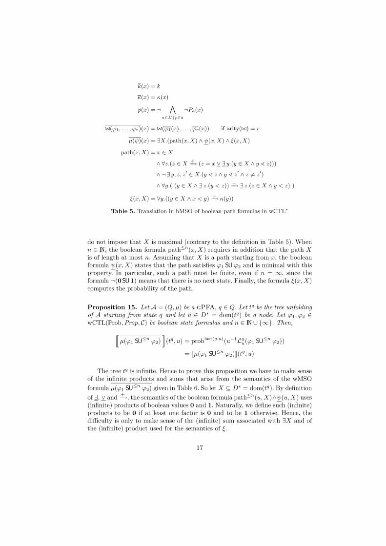
do not impose that X is maximal (contrary to the definition in Table 5). Whenn ∈ N, the boolean formula path≤n(x,X) requires in addition that the path Xis of length at most n. Assuming that X is a path starting from x, the booleanformula ψ(x,X) states that the path satisfies ϕ1 SUϕ2 and is minimal with thisproperty. In particular, such a path must be finite, even if n = ∞, since theformula ¬(0SU1) means that there is no next state. Finally, the formula ξ(x,X)computes the probability of the path.

Proposition 15. Let A = (Q,µ) be a gPFA, q ∈ Q. Let tq be the tree unfoldingof A starting from state q and let u ∈ D∗ = dom(tq) be a node. Let ϕ1, ϕ2 ∈wCTL(Prob,Prop, C) be boolean state formulas and n ∈ N ∪ {∞}. Then,

[[µ(ϕ1 SU

≤n ϕ2)]](tq, u) = problast(q,u)(u−1Lq

u(ϕ1 SU≤n ϕ2))

= [[µ(ϕ1 SU≤n ϕ2)]](t

q, u)

The tree tq is infinite. Hence to prove this proposition we have to make senseof the infinite products and sums that arise from the semantics of the wMSO

formula µ(ϕ1 SU≤n ϕ2) given in Table 6. So let X ⊆ D∗ = dom(tq). By definition

of ∃, ∨ and+−→, the semantics of the boolean formula path≤n(u,X)∧ψ(u,X) uses

(infinite) products of boolean values 0 and 1. Naturally, we define such (infinite)products to be 0 if at least one factor is 0 and to be 1 otherwise. Hence, thedifficulty is only to make sense of the (infinite) sum associated with ∃X and ofthe (infinite) product used for the semantics of ξ.

17

µ(ϕ1 SU≤n ϕ2)(x) = ∃X.(path≤n(x,X) ∧ ψ(x,X) ∧ ξ(x,X))

path≤∞(x,X) = x ∈ X

∧ ∀z.(z ∈ X+−→ (z = x ∨ ∃ y.(y ∈ X ∧ y ⋖ z)))

∧ ¬∃ y, z, z′ ∈ X.(y ⋖ z ∧ y ⋖ z′ ∧ z 6= z

′)

if n ∈ N, path≤n(x,X) = path≤∞(x,X) ∧ ¬∃x0 . . . ∃xn.

(x0 ∈ X ∧ · · · ∧ xn ∈ X ∧ x < x0 < x1 < · · · < xn)

ψ = (ϕ1 ∧ ¬ϕ2) SU (ϕ2 ∧ ¬(0 SU 1))

ξ(x,X) = ∀y.((y ∈ X ∧ x < y)+−→ κ(y))

Table 6. Translation in bMSO of µ(ϕ1 SU≤n ϕ2) ∈ wCTL for n ∈ N ∪ {∞}

Proof (of Prop. 15). We use the notation introduced above. We simply denoteby L the language Lq

u(ϕ1 SU≤n ϕ2) introduced in Section 4:

L = {w ∈ uDω | tq, w, u |= ϕ1 SU≤n ϕ2} .

In this special case, the probability measure problast(q,u)(u−1L) is easy to com-pute. To this aim, we introduce the language

K = {w ∈ uD+ | tq, w, u |= (ϕ1 ∧ ¬ϕ2) SU≤n (ϕ2 ∧ ¬(0 SU 1))}

We can easily check that K is prefix-free: w,w′ ∈ K and w ≤ w′ implies w = w′.Moreover,

L =⊎

w∈K

wDω

and this countable union is disjoint so that

problast(q,u)(u−1L) =∑

w∈K

problast(q,u)(u−1wDω) =∑

w∈K

∏

u<v≤w

κtq(v) .

For each w ∈ uD+, let Xw = {v ∈ D∗ | u ≤ v ≤ w}. Next, define the setX = {Xw ⊆ D∗ | w ∈ K}. One can check that X is precisely the set of subsetsX ⊆ D∗ = dom(tq) such that the formula path≤n(u,X) ∧ ψ(u,X) holds:

[[path≤n ∧ ψ]](tq, u,X) =

{1 if X ∈ X0 otherwise.

Note that the infinite product used in the semantics of [[ξ]](u,X) is always well-defined. Either it has only finitely many factors different from 1 (which is inparticular the case when X is finite) or it converges to 0. For each w ∈ K,[[ξ]](u,Xw) computes the probability of path Xw:

[[ξ]](tq, u,Xw) =∏

u<v≤w

κtq(v) .

18

For sets X /∈ X, we have [[path≤n ∧ ψ ∧ ξ]](tq, u,X) = 0 and we obtain

[[path≤n ∧ ψ ∧ ξ]](tq, u,X) =

{[[ξ]](tq, u,X) if X ∈ X0 otherwise.

Removing 0 terms in an infinite sum, we obtain

[[µ(ϕ1 SU

≤n ϕ2)]](tq, u) = [[∃X.(path≤n ∧ ψ ∧ ξ)]](tq, u)

=∑

X∈X[[ξ]](tq, u,X)

=∑

w∈K

∏

u<v≤w

κtq(v)

= problast(q,u)(u−1L) .

If n ∈ N then the sets K and X are finite and the sums above are finite. Whenn = ∞, i.e., for the natural unbounded strict until, the sets K and X may beinfinite. For instance, this is the case with formula pSUr evaluated on the gPFA

of Figure 3 starting from state q0 where the sets K and X corresponds to theinfinite set of paths q∗0q1. But, as a consequence of the equalities above, theinfinite sums over K and X are well-defined with value in [0, 1]. ⊓⊔

6 Conclusion and open problems

In this paper, we have introduced wMSO, a weighted version of classical MSOlogic. It is interpreted over weighted trees, which naturally appear as unfoldingsof weighted automata. We showed that the satisfiability problem for wMSO isundecidable. We then defined wCTL and wCTL∗ over weighted trees and gavetransformations of these logics into wMSO. For the probabilistic interpretationof the path-quantifier operator µ(ψ), we restricted to a transformation of wCTLinto wMSO formulas.

Let us mention some directions for future work. We need to identify fragmentsof our logic that come with a decidable satisfiability problem. A natural furtherstep is to tackle the model-checking problem: given a weighted formula ϕ anda weighted automaton A, does [[ϕ]](tA) 6= 0 hold? To find a solution, we mightborrow techniques used in the probabilistic setting for PCTL∗. Moreover, thetranslation of wCTL∗ into wMSO remains to be done. For the probabilisticsemantics, such a translation might be based on techniques from [13] developedfor checking linear-time properties of probabilistic systems (see also [5] for anoverview).

It would be worthwhile to add the notion of a scheduler to wMSO to considerunfoldings of (partially observable) MDPs or probabilistic Buchi automata [3,4],which are essentially rPFA with a Buchi acceptance condition.

19

The expectation semiring, defined in [20], combines probabilities with ex-pected rewards. A transfer of our logics to this specific structure (possibly ex-tended by a discount operator) could provide a generic framework for rewardmodels as considered, e.g., in [2, 23].

A weighted µ-calculus has been defined in [22] to be interpreted over quanti-tative Kripke structures. For the design of a weighted µ-calculus over branchingstructures, one might benefit from ideas that led to a weighted µ-calculus overwords [29].

References

1. R. Alur and D. L. Dill. A theory of timed automata. Theoretical Computer Science,126(2):183–235, 1994.

2. S. Andova, H. Hermanns, and J. P. Katoen. Discrete-time rewards model-checked.In Proceedings of FORMATS 2003, volume 2791 of Lecture Notes in Computer

Science, pages 88–104. Springer, 2003.3. C. Baier, N. Bertrand, and M. Großer. On decision problems for probabilistic

Buchi automata. In Proceedings of FoSSaCS’08, volume 4962 of Lecture Notes in

Computer Science, pages 287–301. Springer, 2008.4. C. Baier and M. Großer. Recognizing ω-regular languages with probabilistic au-

tomata. In Proceedings of LICS’05, pages 137–146. IEEE Computer Society Press,2005.

5. B. Bollig and M. Leucker. Verifying qualitative properties of probabilistic pro-grams. In Validation of Stochastic Systems, volume 2925 of Lecture Notes in Com-

puter Science, pages 124–146. Springer, 2004.6. P. Bouyer, U. Fahrenberg, K. G. Larsen, N. Markey, and J. Srba. Infinite runs

in weighted timed automata with energy constraints. In Proceedings of FOR-

MATS’08, volume 5215 of Lecture Notes in Computer Science, pages 33–47.Springer, 2008.

7. P. Buchholz and P. Kemper. Model checking for a class of weighted automata.Discrete Event Dynamic Systems, 2009. to appear.

8. J. R. Buchi. Weak second-order arithmetic and finite automata. Z. Math. Logik

Grundlagen Math., 6:66–92, 1960.9. J. R. Buchi. On a decision method in restricted second order arithmetic. In Proc.

of the International Congress on Logic, Methodology and Philosophy, pages 1–11.Standford University Press, 1962.

10. F. Ciesinski and M. Großer. On probabilistic computation tree logic. In Validation

of Stochastic Systems, volume 2925 of Lecture Notes in Computer Science, pages147–188. Springer, 2004.

11. E. M. Clarke and E. A. Emerson. Design and synthesis of synchronization skele-tons using branching time temporal logic. In Proceedings of the Workshop on Log-

ics of Programs, volume 131 of Lecture Notes in Computer Science, pages 52–71.Springer, 1981.

12. E. M. Clarke, O. Grumberg, and D. Peled. Model Checking. The MIT Press,Cambridge, Massachusetts, 1999.

13. C. Courcoubetis and M. Yannakakis. The complexity of probabilistic verification.Journal of the ACM, 42(4):857–907, 1995.

14. K. Culik and J. Kari. Image compression using weighted finite automata. Computer

and Graphics, 17(3):305–313, 1993.

20

15. L. de Alfaro. Formal verification of probabilistic systems. Technical report, Stan-ford University, 1998. PhD thesis.

16. M. Droste and P. Gastin. Weighted automata and weighted logics. Theoretical

Computer Science, 380(1-2):69–86, 2007. Special issue of ICALP’05.17. M. Droste and P. Gastin. Weighted automata and weighted logics. In W. Kuich,

H. Vogler, and M. Droste, editors, Handbook of Weighted Automata, EATCS Mono-graphs in Theoretical Computer Science. Springer, 2009. To appear.

18. M. Droste and G. Rahonis. Weighted automata and weighted logics with dis-counting. In Proceedings of CIAA’07, volume 4783 of Lecture Notes in Computer

Science, pages 73–84. Springer, 2007.19. M. Droste and H. Vogler. Weighted tree automata and weighted logics. Theoretical

Computer Science, 366(3):228–247, 2006.20. J. Eisner. Expectation semirings: Flexible EM for learning finite-state transducers.

In Proceedings of the ESSLLI workshop on finite-state methods in NLP, 2001.21. C. C. Elgot. Decision problems of finite automata design and related arithmetics.

Trans. Amer. Math. Soc., 98:21–52, 1961.22. D. Fischer, E. Gradel, and L. Kaiser. Model checking games for the quantitative

µ-calculus. Theory of Computing Systems, 2009. Special Issue of STACS 2008.23. M. Großer, G. Norman, C. Baier, F. Ciesinski, M. Kwiatkowska, and D. Parker. On

reduction criteria for probabilistic reward models. In Proceedings of FSTTCS’06,volume 4337 of Lecture Notes in Computer Science, pages 309–320. Springer, 2006.

24. H. Hansson and B. Jonsson. A logic for reasoning about time and reliability. Formal

Aspects of Computing, 6(5):512–535, 1994.25. K. Knopp. Theory and Application of Infinite Series. Dover Publications, New

York, 1990. Republication of the second English edition, 1951.26. D. Kozen. Results on the propositional µ-calculus. Theoretical Computer Science,

27:333–354, 1983.27. W. Kuich and A. Salomaa. Semirings, Automata and Languages. Springer, 1985.28. W. Kuich, H. Vogler, and M. Droste, editors. Handbook of Weighted Automata.

EATCS Monographs in Theoretical Computer Science. Springer, 2009.29. I. Meinecke. A weighted µ-calculus on words. In Proceedings of DLT’09, volume

5583 of Lecture Notes in Computer Science. Springer, 2009. This volume.30. M. Mohri. Finite-state transducers in language and speech processing. Computa-

tional Linguistics, 23(2):269–311, 1997.31. Amir Pnueli. The temporal logic of programs. In Proceedings of FOCS’77, pages

46–57. IEEE Computer Society Press, 1977.32. M. L. Puterman. Markov Decision Processes. John Wiley & Sons, Inc., New York,

NY, 1994.33. M. O. Rabin. Probabilistic automata. Information and Control, 6:230–245, 1963.34. R. Segala. Probability and nondeterminism in operational models of concurrency.

In Proceedings of CONCUR’06, volume 4137 of Lecture Notes in Computer Science,pages 64–78. Springer, 2006.

35. W. Thomas. Languages, automata and logic. In A. Salomaa and G. Rozenberg,editors, Handbook of Formal Languages, volume 3, Beyond Words, pages 389–455.Springer, 1997.

36. R. J. van Glabbeek, S. A. Smolka, and B. Steffen. Reactive, generative and strati-fied models of probabilistic processes. Information and Computation, 121(1):59–80,1995.

37. M. Y. Vardi. Automatic verification of probabilistic concurrent finite-state pro-grams. In Proceedings of FOCS’85, pages 327–338. IEEE, 1985.

21