welcome to physics 331user.physics.unc.edu/~drut/public_html_unc/assets/lecture01.pdf · welcome to...
TRANSCRIPT

Welcome to Physics 331:Introduction to Numerical Techniques in Physics
Instructor: Joaquín Drut
Lecture 1

Logistics…
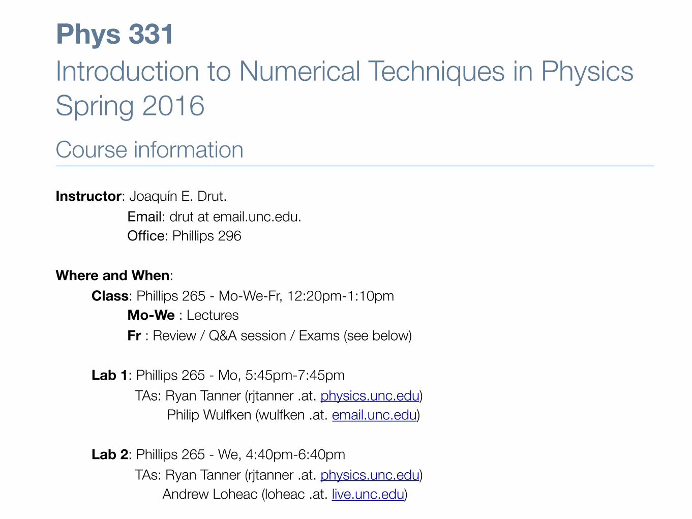
Phys 331
Introduction to Numerical Techniques in Physics
Spring 2016
Course information
Instructor: Joaquín E. Drut.
Email: drut at email.unc.edu.
Office: Phillips 296
Where and When:
Class: Phillips 265 - Mo-We-Fr, 12:20pm-1:10pm
Mo-We : Lectures
Fr : Review / Q&A session / Exams (see below)
Lab 1: Phillips 265 - Mo, 5:45pm-7:45pm
TAs: Ryan Tanner (rjtanner .at. physics.unc.edu)
Philip Wulfken (wulfken .at. email.unc.edu)
Lab 2: Phillips 265 - We, 4:40pm-6:40pm
TAs: Ryan Tanner (rjtanner .at. physics.unc.edu) Andrew Loheac (loheac .at. live.unc.edu)
Office hours: By appointment only.
To obtain an appointment, email me directly. Your subject heading must begin with Phys331.
Website: http://user.physics.unc.edu/~drut/public_html_UNC/physics-331.html
Bibliography: - A. Gilat & V. Subramaniam, Numerical Methods for Engineers and Scientists. - Press, Teukolsky, Vetterling, Flannery, Numerical recipes in C (2nd Edition, 1992). - M.L. Boas, Mathematical Methods in the Physical Sciences.
Software: MATLAB
Midterm 1: Friday, February 12th (in class).
Midterm 2: Friday, March 11th (in class).
Final Exam: Saturday, April 30th, 12pm, Phillips 265

How to get MATLAB
https://software.sites.unc.edu/software/matlab/
Follow this link:
Or use our instructions here:http://user.physics.unc.edu/~drut/public_html_UNC/assets/matlabinstructions.pdf

Important dates
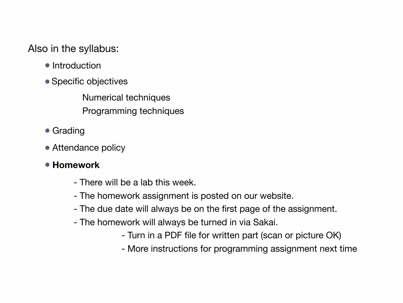
Also in the syllabus:IntroductionSpecific objectives
Grading
Numerical techniquesProgramming techniques
Homework
Attendance policy
- There will be a lab this week.- The homework assignment is posted on our website.- The due date will always be on the first page of the assignment.- The homework will always be turned in via Sakai. - Turn in a PDF file for written part (scan or picture OK) - More instructions for programming assignment next time
Why numerical techniques?

Why are you here?
Many (in fact most) problems do not have a closed-form analytic solution
For example...
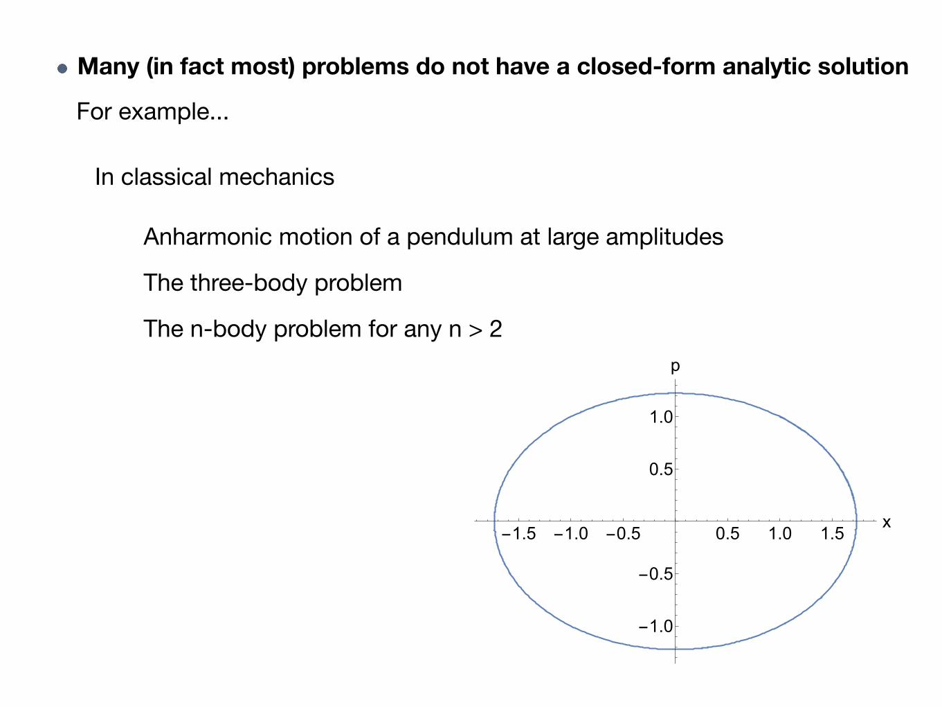
Many (in fact most) problems do not have a closed-form analytic solution
For example...
In classical mechanics
Anharmonic motion of a pendulum at large amplitudes
The three-body problem
The n-body problem for any n > 2
-1.5 -1.0 -0.5 0.5 1.0 1.5x
-1.0
-0.5
0.5
1.0
p

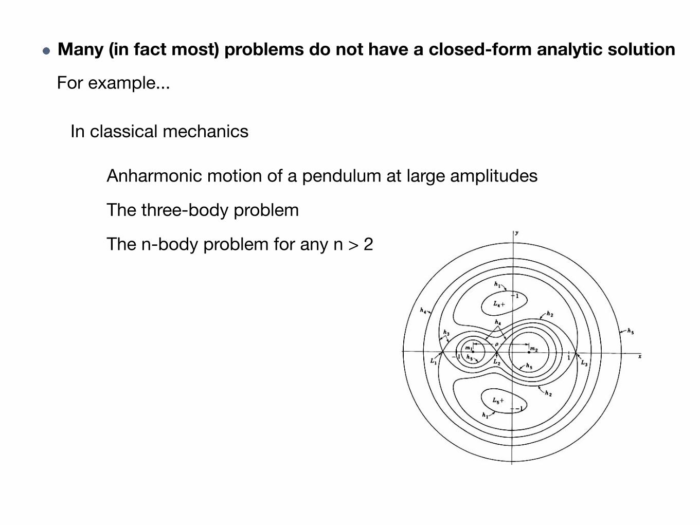
Many (in fact most) problems do not have a closed-form analytic solution
For example...
In classical mechanics
Anharmonic motion of a pendulum at large amplitudes
The three-body problem
The n-body problem for any n > 2
-5 -4 -3 -2 -1 1 2x
-1.0-0.5
0.51.0p
Many (in fact most) problems do not have a closed-form analytic solution
For example...
In classical mechanics
Anharmonic motion of a pendulum at large amplitudes
The three-body problem
The n-body problem for any n > 2
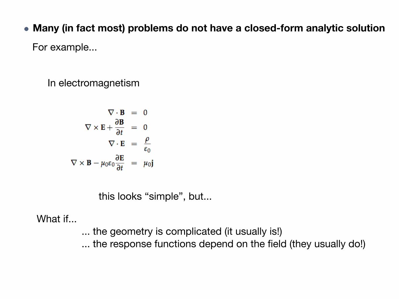
Many (in fact most) problems do not have a closed-form analytic solution
For example...
In electromagnetism
this looks “simple”, but...
What if... ... the geometry is complicated (it usually is!) ... the response functions depend on the field (they usually do!)

Many (in fact most) problems do not have a closed-form analytic solution
For example...
In electromagnetism
this looks “simple”, but...
What if... ... the geometry is complicated (it usually is!) ... the response functions depend on the field (they usually do!)

Many (in fact most) problems do not have a closed-form analytic solution
For example...
In electromagnetism
this looks “simple”, but...
What if... ... the geometry is complicated (it usually is!) ... the response functions depend on the field (they usually do!)
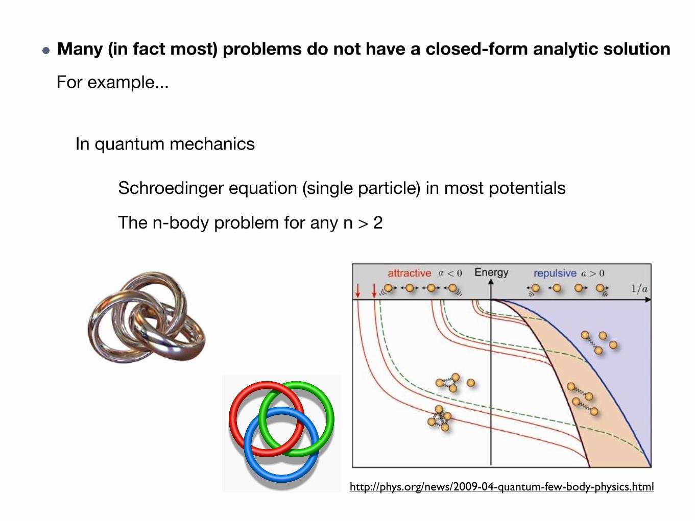
Many (in fact most) problems do not have a closed-form analytic solution
For example...
In quantum mechanics
Schroedinger equation (single particle) in most potentials
The n-body problem for any n > 2
http://phys.org/news/2009-04-quantum-few-body-physics.html

Many (in fact most) problems do not have a closed-form analytic solution
For example...
In quantum field theory
Pretty much any interacting theory in 2D and 3D
http://www.lattice-qcd.org/

Many (in fact most) problems do not have a closed-form analytic solution
Some solutions require repetitive tasks
For example...
Systems of linear equations
Root-finding
Integration
12.4x+ 37y + 238.45z = 20
1.6x+ 123y + 19.1z = 1
3.4x+ e
6.2y + 7.65z = ⇡
Image source: wikimedia commons
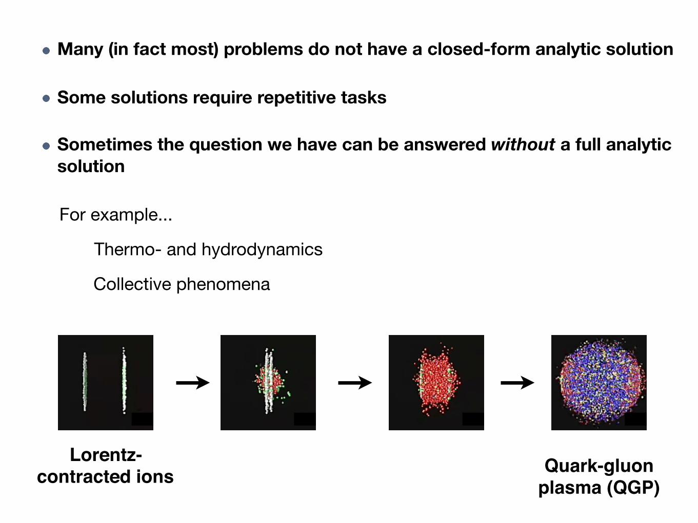
Many (in fact most) problems do not have a closed-form analytic solution
Some solutions require repetitive tasks
Sometimes the question we have can be answered without a full analytic solution
For example...
Collective phenomena
Thermo- and hydrodynamics
Lorentz-contracted ionsbefore collision
Quark-gluon plasma (QGP)
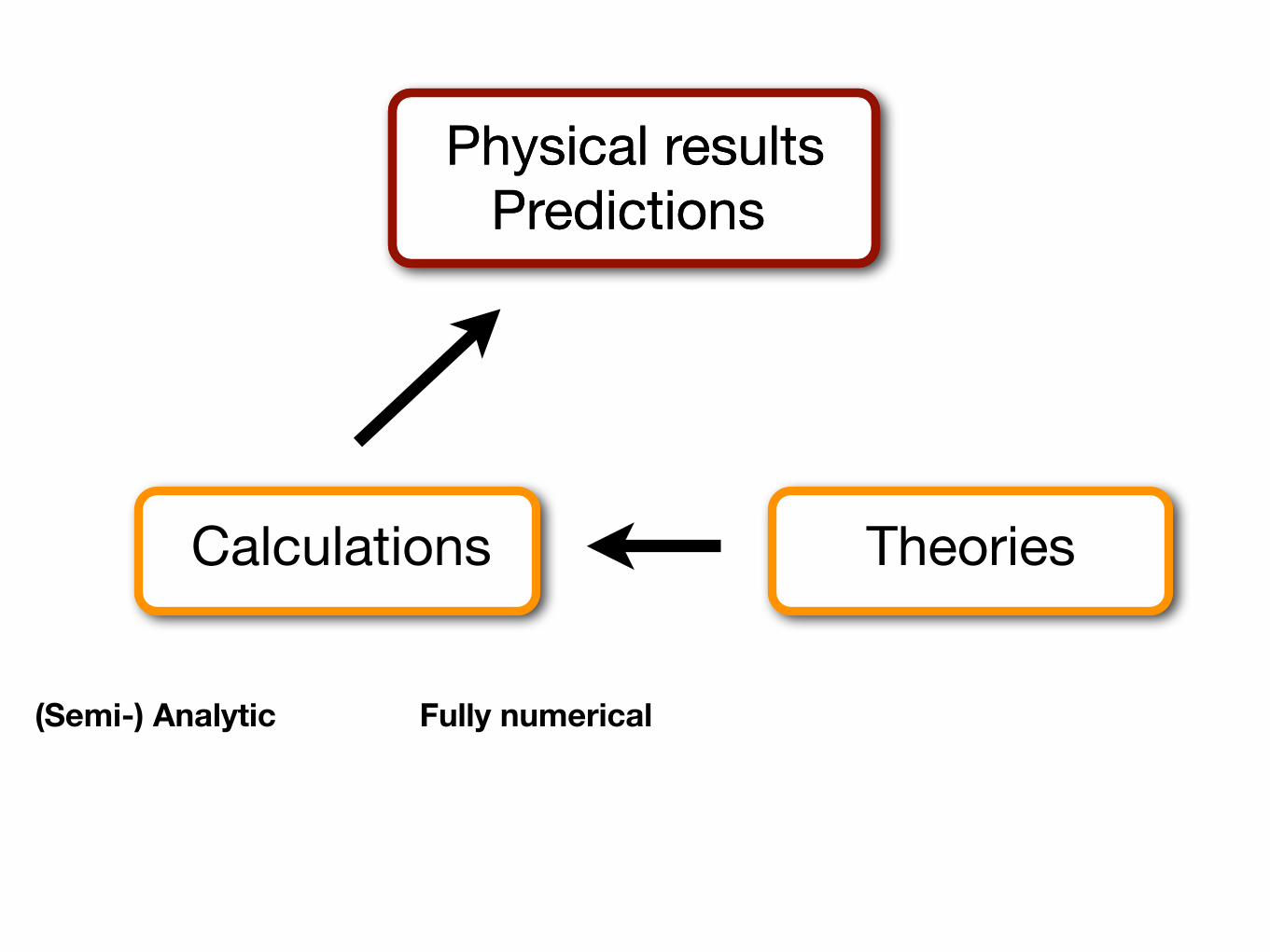
Physical results Predictions
Calculations
Physical results Predictions
Theories
Fully numerical(Semi-) Analytic

What you will get from this course (hopefully)

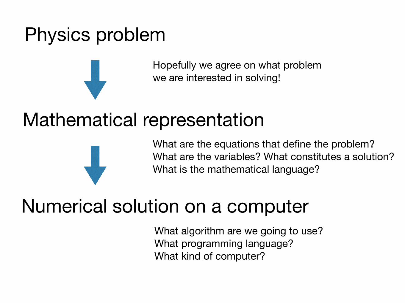
Physics problem
Mathematical representation
Numerical solution on a computer
Hopefully we agree on what problem we are interested in solving!
What are the equations that define the problem?What are the variables? What constitutes a solution?What is the mathematical language?
What algorithm are we going to use?What programming language?What kind of computer?

Mathematics reviewChapter 2 in Gilat and Subramaniam.If any of this sounds daunting or too foreign, you may want to: a) consider taking this course another time; b) read chapter 2 now as fast as you can.
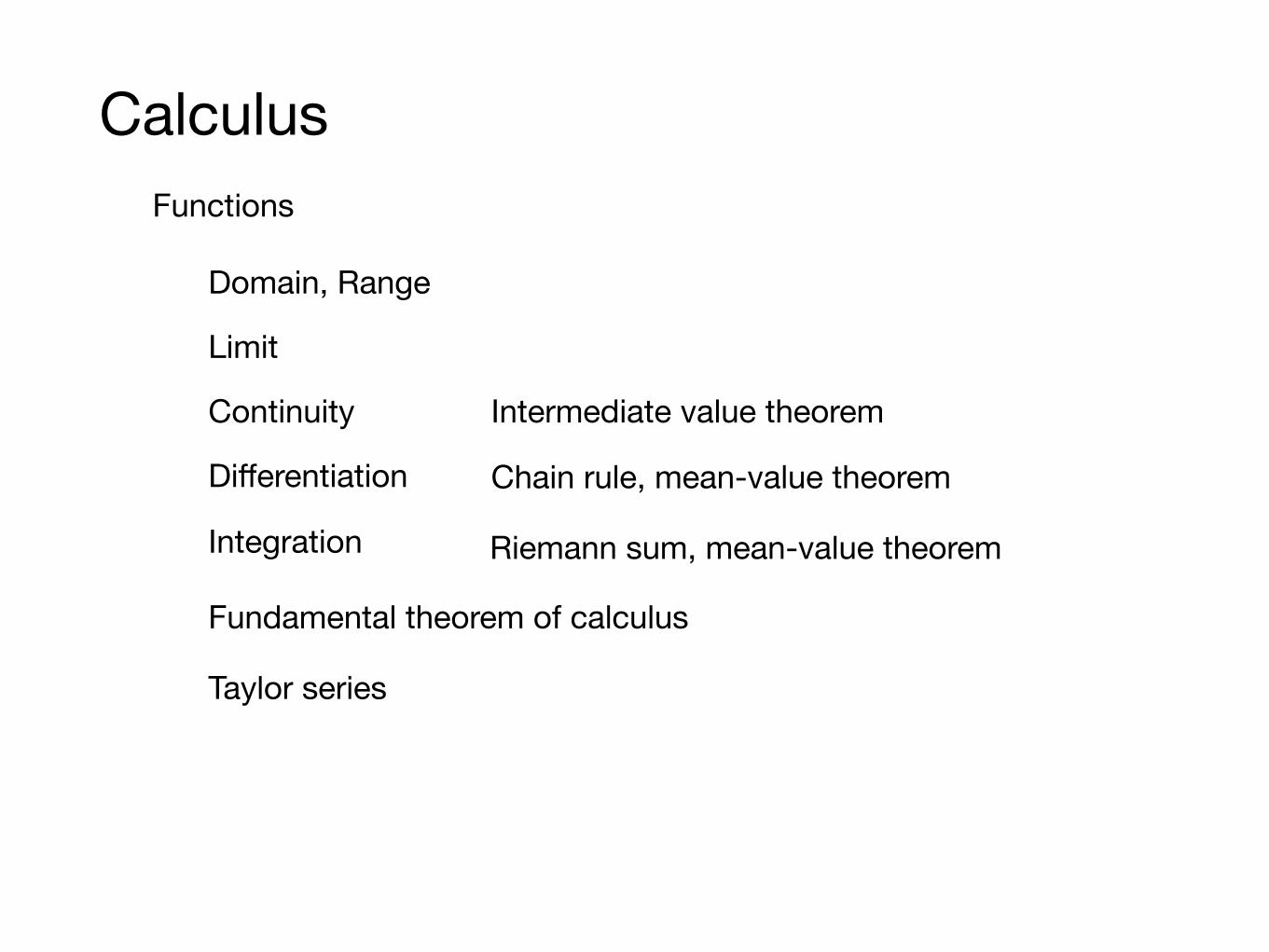
CalculusFunctions
Domain, Range
Limit
Continuity
Differentiation
Intermediate value theorem
Chain rule, mean-value theorem
Integration
Fundamental theorem of calculus
Riemann sum, mean-value theorem
Taylor series
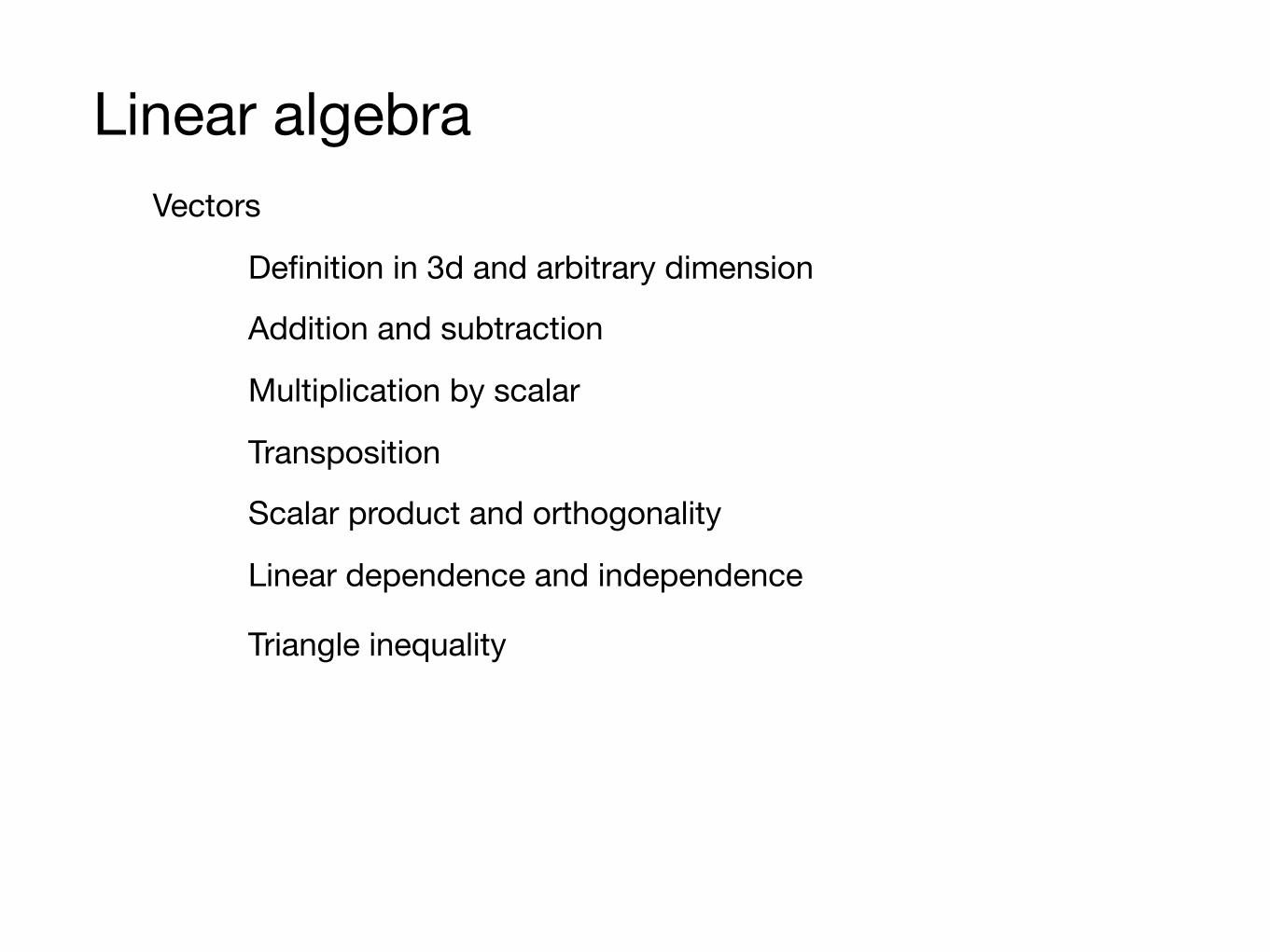
Linear algebraVectors
Definition in 3d and arbitrary dimension
Addition and subtraction
Multiplication by scalar
Transposition
Scalar product and orthogonality
Linear dependence and independence
Triangle inequality
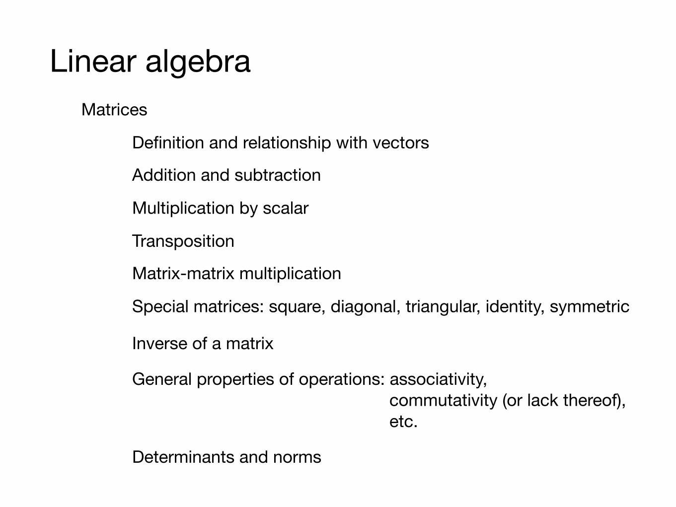
Linear algebraMatrices
Definition and relationship with vectors
Addition and subtraction
Multiplication by scalar
Transposition
Matrix-matrix multiplication
Special matrices: square, diagonal, triangular, identity, symmetric
Inverse of a matrix
General properties of operations: associativity, commutativity (or lack thereof), etc.
Determinants and norms

Differential equationsLinear vs. non-linear
Homogeneous vs. inhomogeneous
Order
Analytic solutions

Multivariable calculusFunctions of more than one variable
Partial derivatives
Chain rule
Taylor series expansion
Next time:
Reading:
Introduction - Chapter 1
Sources of error
First steps in MATLAB
Number representation