Welfare and Optimal Trading Frequency in

Dynamic Double Auctions∗

Songzi Du† Haoxiang Zhu‡

This version: September 14, 2014First version: May 2012

∗Earlier versions of this paper were circulated under the titles “Ex Post Equilibria in DoubleAuctions of Divisible Assets” and “Dynamic Ex Post Equilibrium, Welfare, and Optimal TradingFrequency in Double Auctions”. For helpful comments, we are grateful to Alexis Berges, BrunoBiais, Alessandro Bonatti, Bradyn Breon-Drish, Jeremy Bulow, Hui Chen, David Dicks, DarrellDuffie, Thierry Foucault, Willie Fuchs, Lawrence Glosten, Lawrence Harris, Joel Hasbrouck, TerryHendershott, Eiichiro Kazumori, Ilan Kremer, Martin Lettau, Stefano Lovo, Andrey Malenko, KatyaMalinova, Gustavo Manso, Konstantin Milbradt, Sophie Moinas, Michael Ostrovsky, Jun Pan, An-dreas Park, Parag Pathak, Michael Peters, Paul Pfleiderer, Uday Rajan, Marzena Rostek, IoanidRosu, Gideon Saar, Andy Skrzypacz, Chester Spatt, Juuso Toikka, Dimitri Vayanos, Jiang Wang,Yajun Wang, Bob Wilson, and Liyan Yang, Hayong Yun, as well as seminar participants at Stan-ford University, Simon Fraser University, MIT, Copenhagen Business School, University of BritishColumbia, UNC Junior Finance Faculty Roundtable, Midwest Theory Meeting, Finance TheoryGroup Berkeley Meeting, Canadian Economic Theory Conference, HEC Paris, Econometric SocietySummer Meeting, Barcelona Information Workshop, CICF, Stony Brook Game Theory Festival,SAET, Bank of Canada, Carnegie Mellon Tepper, University of Toronto, NBER Microstructuremeeting, IESE Business School, Stanford Institute for Theoretical Economics, UBC Summer Work-shop in Economic Theory, and Toulouse Conference on Trading in Electronic Market. Paper URL:http://ssrn.com/abstract=2040609.†Simon Fraser University, Department of Economics, 8888 University Drive, Burnaby, B.C.

Canada, V5A 1S6. songzid@sfu.ca.‡MIT Sloan School of Management and NBER, 100 Main Street E62-623, Cambridge, MA 02142.

zhuh@mit.edu.

Welfare and Optimal Trading Frequency inDynamic Double Auctions

September 14, 2014

Abstract

This paper studies the welfare consequence of increasing trading speed in finan-

cial markets. We build and solve a dynamic trading model, in which traders

receive private information of asset value over time and trade strategically with

demand schedules in a sequence of double auctions. A stationary linear equi-

librium and its efficiency properties are characterized explicitly in closed form.

Slow trading (few double auctions per unit of time) serves as a commitment

device that induces aggressive demand schedules, but fast trading allows more

immediate reaction to new information. If all traders have the same speed,

the socially optimal trading frequency tends to be low for scheduled arrivals

of information but high for stochastic arrivals of information. If traders have

heterogeneous trading speed, fast traders prefer the highest feasible trading

frequency, whereas slow traders tend to prefer a strictly lower frequency.

Keywords: trading frequency, welfare, high-frequency trading, dynamic trading,

double auction

JEL Codes: D44, D82, G14

1

1 Introduction

Trading in financial markets has become significantly faster over the last decade.

Today, electronic transactions for equities, futures, and foreign exchange are typically

conducted within millisecond or microseconds.1 Electronic markets, which typically

have a higher speed than manual markets, are also increasingly adapted in the over-

the-counter markets for debt securities and derivatives, such as corporate bonds,

interest rates swaps, and credit default swaps.2 Exchange traded funds, which trade

at a high frequency like stocks, have gained significant market shares over index

mutual funds, which only allow buying and selling at the end of day.3

The remarkable speedup in financial markets raises important economic questions.

For example, does a higher speed of trading necessarily lead to a higher social welfare,

in terms of more efficient allocations of assets? What is the socially optimal frequency

(if one exists) at which financial markets should operate? Moreover, given that certain

investors trade at a higher speed than others, does a higher trading frequency affect

fast investors and slow ones equally or differentially? Answers to these questions

would provide valuable insights for the ongoing academic and policy debate on market

structure, especially in the context of high-frequency trading.4

In this paper, we set out to investigate the welfare consequence of speeding up

trading in financial markets. We build and solve a dynamic model with strategic

trading, adverse selection, and imperfect competition. Specifically, in our model, a

finite number (n ≥ 3) of investors trade a divisible asset in an infinite sequence of

1A millisecond is a thousandth of a second, and a microsecond is a millionth of a second. In eq-uity markets, for example, NASDAQ reports that its system can currently handle a message within40 microseconds; see http://www.nasdaqtrader.com/Trader.aspx?id=Latencystats. In futures mar-ket, CME reports that the median inbound latency on its system is about 52 microseconds; seehttp://www.cmegroup.com/globex/files/globexbrochure.pdf. EBS Market, a major electronic trad-ing platform for foreign exchange, introduced a speed delay of up to 3 milliseconds to incomingorders in August 2013; see “EBS take new step to rein in high-frequency traders,” by Wanfeng Zhouand Nick Olivari, Reuters, August 23, 2013.

2For example, the Dodd-Frank Act of United States Congress has mandated that standardizedover-the-counter derivatives must be traded on “swap execution facilities,” which are effectivelyelectronic “mini-exchanges.” These derivatives used to be traded by manual quotation and execution.

3See, for instance, “ETFs Gain Ground on Index Mutual Funds,” by Murray Coleman, WallStreet Journal, February 20, 2014.

4For example, Securities and Exchange Commission (2010) provides an excellent review of eco-nomic questions and policy issues on U.S. equity market structure. In early 2014, European regu-lators adopted the Markets in Financial Instruments Directive (MiFID) II, which set out principlesand regulations for many aspects of European financial markets. The rise of high-frequency tradingis a key issue in both.

2

uniform-price double auctions, held at discrete time intervals. The shorter is the time

interval between auctions, the higher is the speed of the market. At an exponentially-

distributed time in the future, the asset pays a liquidating dividend, which, until

that payment time, evolves according to a jump process. Traders receive over time

informative signals of dividend shocks, as well as shocks to their private values for

owning the asset. Traders also incur quadratic costs for holding inventories, which is

equivalent to linearly decreasing marginal values. A trader’s dividend signals, shocks

to his private values, and his inventories are all his private information. In each

double auction, traders submit demand schedules (i.e., a set of limit orders) and pay

for their allocations at the market-clearing price. All traders take into account the

price impact of their trades.

Our model incorporates many salient features of dynamic markets in practice. For

example, information about the common dividend captures adverse selection, whereas

private-value information and convex holding costs introduce gains from trade. These

trading motives are also time-varying as news arrives over time. Moreover, the number

of double auctions per unit of clock time is a simple yet realistic way to model trading

frequency in dynamic markets (see the literature section for more discussion of this

modeling approach).

A dynamic equilibrium and efficiency

The first primary result of this paper is to characterize a linear stationary equilibrium

of this dynamic market and its efficiency properties. In equilibrium, a trader’s optimal

demand in each double auction is a linear function of the price, his signal of the

dividend, his most recent private value, and his private inventory. Each coefficient is

solved explicitly in closed form. Naturally, the equilibrium price in each auction is a

weighted sum of the average signal of the common dividend and the average private

value, adjusted for the marginal holding cost of the average inventory. Prices are

martingales since the innovations in common dividend and private values have zero

mean.

Because there are a finite number of traders, demand schedules in this dynamic

equilibrium are not competitive. Consequently, the equilibrium allocations of assets

across traders after each auction are not fully efficient, but they converge gradually

and exponentially over time to the efficient allocation. This convergence remains slow

and gradual even in the continuous-time limit. We show that the convergence rate

3

per unit of clock time increases with the number of traders, the arrival intensity of the

dividend, the variance of the private-value shocks, and the trading frequency of the

market; but the convergence rate decreases with the variance of the common-value

shocks, which is a measure of adverse selection.

Furthermore, equilibrium allocations also converge to the efficient level as the

the number n of traders increases. A novel result from our analysis is that ad-

verse selection—asymmetric information about the common dividend—slows down

this convergence rate. Without the adverse selection, allocative inefficiency van-

ishes at the rate O(n−2), but with adverse selection, inefficiency vanishes at the rate

O(n−4/3). In the continuous-time limit, the respective convergence rates are O(n−1)

and O(n−2/3).

Welfare and optimal trading frequency

Our modeling framework proves to be an effective tool in answering welfare questions.

Characterizing welfare and optimal trading frequency in this dynamic market is the

second primary contribution of our paper.

We ask two related questions regarding trading frequency. First, what is the

socially optimal trading frequency if all traders have equal speed? Second, if certain

traders are faster than others, what are the trading frequencies that are optimal for

fast and slow traders respectively?

The first question on homogenous speed can be readily analyzed in our benchmark

model, in which all traders participate in all double auctions. We emphasize that a

change of trading frequency in our model does not change the fundamental properties

of the asset, such as the timing and magnitude of the dividend shocks. Increasing

trading frequency involves an important tradeoff. On the one hand, a higher trading

frequency allows traders to react more quickly to new information and to trade sooner

toward the efficient allocation. This effect favors a faster market. On the other hand,

a lower trading frequency serves as a commitment device that induces aggressive

demand schedules, which leads to more efficient allocations in early rounds of trading.

This effect favors a slow market. The optimal trading frequency should provide the

best balance between minimizing delay in reacting to new information and maximizing

the aggressiveness of demand schedules.

We show that depending on the nature of information arrivals, this tradeoff leads

to different optimal trading frequencies. If new information of dividend and private

4

values arrives at scheduled time intervals, we show that the optimal trading frequency

cannot be higher than the frequency of new information. Hence, slow trading tends to

be optimal. If, instead, new information arrives at Poisson times, faster trading tends

to be optimal. In particular, if the initial inventories are efficient given the time-0

information, continuous trading is optimal under Poisson information arrivals. For

both scheduled and stochastic arrivals of information, the more volatile is the potential

change in the efficient allocation, the higher is the optimal trading frequency.

To answer the second question of welfare, we build an extension of our model to

allow for heterogeneous trading speed. In this extension, a fast trader accesses the

market whenever it is open, but a flow of discrete slow traders access the market only

once. Different from recent studies of high-frequency trading (see literature part), we

do not endow the fast trader with any information advantage.

We find that the fast and slow traders tend to prefer different trading frequen-

cies. Because of his frequent access to the market, the fast trader in our model plays

the endogenous role of intermediating trades among slow traders who arrive sequen-

tially. Through this intermediation the fast trader extracts rents. A higher trading

frequency reduces the number of slow traders in each double auction, making the

market “thinner” and the fast trader’s rents higher. We show that the optimal trad-

ing frequency for the fast trader is such that there are exactly two slow traders in

each trading round, which is the highest feasible frequency under the constraint that

the number of traders in each round is an integer. By contrast, slow traders typically

prefer a strictly lower trading frequency (and a thicker market) because they benefit

from pooling trading interests over time and providing liquidity to each other.

Relation to the literature

Our results contribute to two broad branches of literature: dynamic trading with

demand schedules and the welfare effect of trading frequency.

Dynamic trading with demand schedules. Existing papers on dynamic trading

with demand schedules have mostly focused on private information of inventories or

private values. For example, Vayanos (1999) studies a dynamic market in which the

asset fundamental value (dividend) is public information, but agents receive periodic

inventory shocks. Rostek and Weretka (2014) study dynamic trading with multiple

dividend payments, but traders in their model have symmetric information of the as-

set’s fundamental. Sannikov and Skrzypacz (2014) analyze a continuous-time trading

5

model in which traders have asymmetric risk capacity and private inventory shocks,

but no asymmetric information for the common value of the asset. (Sannikov and

Skrzypacz consider common value in an extension.)

Relative to these three papers, a primary distinction of our paper is that we

address adverse selection, i.e., asymmetric information regarding the common value

(component) of the asset.5 Adverse selection matters for the speed of convergence

to efficiency. For a fixed n, the convergence to efficiency over time is slowed down

by adverse selection. As the market becomes large (i.e., n → ∞), the asymptotic

convergence rate with adverse selection is O(n−4/3), slower than the convergence rate

without adverse selection, O(n−2). The O(n−2) convergence rate is also obtained by

Vayanos (1999) in a model with commonly observed dividends.

Kyle, Obizhaeva, and Wang (2013) study a continuous-time trading model in

which agents have pure common values but “agree to disagree” on the precision of

their signals. Because trading in their model happens only in continuous time, Kyle,

Obizhaeva, and Wang (2013) do not address the welfare effect of trading frequency.

Their focus is non-martingale price dynamics, such as price spikes and reversals.

More broadly, our paper is related to the microstructure literature on informed

trading, most notably Kyle (1985) and Glosten and Milgrom (1985), as well as many

extensions.6 This literature predominantly assumes the presence of noise traders,

which makes it difficult to analyze welfare. Dynamic models based on rational ex-

pectations equilibrium (REE) assume price-taking behavior,7 whereas traders in our

model fully internalize the impacts of their trades on the equilibrium price.

Welfare consequences of trading frequency. The literature has two general ap-

proaches to modeling the welfare consequence of trading frequency. Under the first

approach, all investors trade at the same speed. Under the second approach, certain

investors are faster than others. Our results contribute to both.

On homogeneous trading speed, Vayanos (1999) finds that if the inventory shocks

are private information and are small, then a lower trading frequency is better for

welfare.8 Confirming Vayanos’s result, we show that under scheduled information

5Private information regarding the common value or interdependent value of the asset is addressedin prior static models with demand schedules, such as Kyle (1989), Vives (2011), Rostek and Weretka(2012), and Babus and Kondor (2012), among others.

6Recent dynamic extensions of Kyle (1985) include Foster and Viswanathan (1996), Back, Cao,and Willard (2000), and Ostrovsky (2012), among many others.

7See, for example, He and Wang (1995) and Biais, Bossaerts, and Spatt (2010), based on theseminal work of Grossman and Stiglitz (1980) and Grossman (1976, 1981).

8Vayanos (1999) also shows that if inventory information is common knowledge, there is a con-

6

arrivals slower trading tends to be optimal. We share the intuition and underlying

mechanism with Vayanos (1999) that a lower trading frequency serves as a commit-

ment device that encourages traders to submit aggressive demand schedules.

Different from Vayanos’s result, however, we characterize natural conditions under

which fast trading tends to be optimal. Specifically, if new information arrives at

stochastic times, too low a trading frequency prevents traders from reacting to new

information quickly, thus reducing welfare. In this case, the cost of failing to react

to new information can overweigh the benefit of more aggressive demand schedules.

Fast trading can be optimal as a result. Under explicitly characterized conditions,

the optimal trading frequency can be arbitrarily high.

Fuchs and Skrzypacz (2013) consider a bargaining-based model with many com-

petitive one-time buyers and a single seller who has private information. They show

that an “early closure” of market improves welfare relative to continuous trading.

Our result differs in that we characterize explicit conditions under which the optimal

trading frequency can be (arbitrarily) high.

On heterogeneous trading speed, our paper is complementary to existing studies on

the welfare consequences of high-frequency trading.9 In the model of Biais, Foucault,

and Moinas (2014), fast traders have higher transaction probabilities but also possess

superior information regarding the fundamental value of the asset. Pagnotta and

Philippon (2013) model the speed competition by multiple markets, where speed is

defined as the rate of contacts among investors. Budish, Cramton, and Shim (2013)

argue that high-frequency traders simply “arbitrage” public information by picking

off stale quotes, and suggest frequent batch auctions as a market design (as opposed

to a continuous market). Hoffmann (2014) models a limit order market in which the

fast traders can cancel orders (e.g. after asset value shocks) but slow traders cannot.

All four papers ask the welfare question of whether investment in high-speed trading

technology is socially wasteful. Jovanovic and Menkveld (2012) model high-frequency

tinuum of equilibria. Under one of these equilibria, selected by a trembling hand refinement, welfareis increasing in trading frequency. Because our model has private information of inventories, theprivate-information equilibrium of Vayanos (1999) is a more appropriate benchmark for comparison.Related, Rostek and Weretka (2014) consider a market in which: (i) information of asset value issymmetric among agents and (ii) between consecutive dividend payments there is no news and nodiscounting. In this setting, they show that a higher trading frequency is better for welfare.

9Recent studies that model high-frequency trading, but do not address the associated welfare,include Foucault, Hombert, and Rosu (2013), Baruch and Glosten (2013), Rosu (2014), Yueshen(2014), Li (2014), Menkveld and Zoican (2014), Aıt-Sahalia and Saglam (2014), and Foucault,Kozhan, and Tham (2014), among others.

7

traders as informed intermediaries whose presence can reduce or create information

frictions, and study to what extent high-frequency traders increase or reduce gains

from trade.

Different from these studies, fast traders in our model has no informational ad-

vantage; their only advantage is having more frequent access to the market than slow

traders. Still, we show that the fast trader extracts rents by intermediating trades

among slow traders. Moreover, our welfare question focuses on how trading frequency

interacts with imperfect competition and hence the efficient allocations of assets.

2 Dynamic Trading in Double Auctions

This section presents the dynamic trading model and characterizes the equilibrium

and its properties. Main model parameters are tabulated in Appendix A for ease of

reference.

2.1 Model

Timing and asset. Time is continuous, τ ∈ [0,∞). A divisible asset is trading on

the market. The asset pays a single liquidating dividend D at some exponential time

T with the associated intensity r > 0. The random dividend time T is independent

of all else in the model. The dividend D starts at D0 at time T0 = 0, where D0 ∼N (0, σ2

D). Moreover, conditional on the dividend time T having not arrived, the

dividend is shocked at the consecutive clock times T1, T2, T3, . . . . The shock times

{Tk}k≥1 can be deterministic or stochastic. The shocks to the dividend at each time

in {Tk}k≥1 are also i.i.d. normal with mean 0 and variance σ2D:

DTk −DTk−1∼ N (0, σ2

D). (1)

Thus, before the dividend is paid out, the “latent” dividend process {Dτ}τ≥0 follows

a jump process:

Dτ = DTk , if Tk ≤ τ < Tk+1. (2)

If the dividend payment time T happens at time τ , the realized dividend will be Dτ .

Since the expected dividend payment time is finite (with mean 1/r), for simplicity

we normalize the interest rate to be zero (i.e., there is no time discounting). Allowing

time discounting does not change our qualitative results.

8

Trading in double auctions. There are n ≥ 3 risk-neutral traders in this market.

Trading is organized as a sequence of uniform-price divisible double auctions. The

double auctions happen at clock times {0,∆, 2∆, 3∆, . . .}, where ∆ > 0 is the length

of clock time between consecutive rounds of trading. The trading frequency is the

number of double auctions per unit of time, i.e., 1/∆. The smaller is ∆, the higher

is the trading frequency. We will refer to each trading round as a “period,” indexed

by t ∈ {0, 1, 2, . . .}, so period-t trading occurs at clock time t∆.

We denote by zi,t∆ the inventory held by trader i immediately before the period-

t double auction. The initial inventories zi,0 are given exogenously, and the total

initial inventory Z ≡∑

i zi,0 is common knowledge. (In securities markets, Z can

be interpreted as the total asset supply. In derivatives markets, Z is by definition

zero.) In period t each trader submits a demand schedule xi,t∆(p) : R → R. The

market-clearing price in period t, p∗t∆, satisfies

n∑i=1

xi,t∆(p∗t∆) = 0. (3)

In the equilibrium we characterize later, the demand schedules are strictly downward-

sloping in p and the solution p∗t∆ is unique. The evolution of inventory is given by

zi,(t+1)∆ = zi,t∆ + xi,t∆(p∗t∆). (4)

After the period-t double auction, each trader i receives xi,t∆(p∗t∆) units of the assets

at the price of p∗t∆ per unit. (A negative xi,t∆(p∗t∆) means selling the asset.)

Information and preference. At clock time Tk, k ∈ {0, 1, 2, · · · }, each trader i

receives a private signal Si,Tk about the dividend shock:

Si,Tk = DTk −DTk−1+ εi,Tk , where εi,Tk ∼ N (0, σ2

ε ) are i.i.d., (5)

and where DT−1 = 0. We also refer to Tk’s as “news times.” The private signals of

trader i are never disclosed to anyone else.

In addition, each trader i has a private-value component wi,T for receiving the

dividend. For example, this private component can reflect tax or risk-management

considerations. Specifically, at each time Tk, k ∈ {0, 1, 2, · · · }, trader i receives a

9

shock to his private value for the asset such that:

wi,Tk − wi,Tk−1∼ N (0, σ2

w), i.i.d., (6)

where wi,T−1 = 0. Written in continuous time, the private-value process wi,τ for trader

i is a jump process:

wi,τ = wi,Tk , if Tk ≤ τ < Tk+1. (7)

The private values to trader i are observed by himself and are never disclosed to

anyone else.

Moreover, in an interval [t∆, (t + 1)∆) but before the dividend D is paid, trader

i incurs a “flow cost” that is equal to 0.5λz2i,(t+1)∆ per unit of clock time, where

λ > 0 is a commonly known constant. The quadratic flow cost is essentially a dy-

namic version of the quadratic cost used in the static models of Vives (2011) and

Rostek and Weretka (2012). We can also interpret this flow cost as an inventory

cost, which can come from regulatory capital requirements, collateral requirement,

or risk-management considerations. (This inventory cost is not strictly risk aversion,

however.10) Once the dividend is paid out in cash, the flow cost no longer applies.

By the exponential distribution of T , conditional on the dividend is not yet paid by

time t∆, the expected length of time during which the flow cost is incurred in period

t is

(1− e−r∆)

∫ ∆

0

re−rτ

1− e−r∆τ dτ + e−r∆∆ =

1− e−r∆

r. (8)

For conciseness of expressions we let Hi,τ be the “history” (information set) of

trader i at time τ :

Hi,τ = {(Si,Tl , wi,Tl)}Tl≤τ ∪ {zt′∆}t′∆≤τ ∪ {xi,t′∆(p)}t′∆<τ . (9)

That is, Hi,τ contains trader i’s asset value-relevant information received up to time τ ,

trader i’s path of inventories up to time τ , and trader i’s demand schedules in double

auctions before time τ . Notice that by the identity zi,(t′+1)∆ − zi,t′∆ = xi,t′∆(p∗t′∆), a

10While it would be desirable to find a formal link between this linear-quadratic preference anda conventional CARA-normal setting, this equivalence has not been obtained. We are not aware ofstudies that formally link CARA-normal setting to linear-quadratic preference under (i) a dynamicmarket, (ii) strategic trading with demand schedules, and (iii) adverse selection. Vayanos (1999)and Rostek and Weretka (2014) use the CARA-normal setting, although their model has no adverseselection.

10

trader can infer the price in the past period t′ from Hi,τ .

We define the “time-τ ex post value” of trader i at τ , conditional on trader i’s

history and all other traders’ history, as:

vi,τ = wi,τ + E [Dτ | Hi,τ ∪ {Hj,τ}j 6=i] . (10)

Thus, trader i’s time-t∆ ex post value for holding the quantity zi,t∆ + xi,t∆(p∗t∆),

evaluated at time t∆ immediately after the period-t auction, is vi,t∆(zi,t∆+xi,t∆(p∗t∆)).

We call vi,τ the “time-τ ex post value” because we have conditioned on {Hj,τ}j 6=i,which is not observed by trader i. But vi,τ is not the realized ex post value because

the dividend is not yet paid.

We define trader i’s “period-t ex post utility” immediately after the double auction

at time t∆ by the recursive equation:

Vi,t∆ =− x∗i,t∆p∗t∆ + (1− e−r∆)vi,t∆(zi,t∆ + x∗i,t∆)− 1− e−r∆

r· λ

2(zi,t∆ + x∗i,t∆)2

+ e−r∆E[Vi,(t+1)∆ | Hi,t∆ ∪ {Hj,t∆}j 6=i

], (11)

where x∗i,t∆ is a shorthand for xi,t∆(p∗t∆). We call Vi,t∆ the “period-t ex post utility”

because we have conditioned on Hi,t∆ ∪ {Hj,t∆}j 6=i, but Vi,t∆ is not trader i’s realized

ex post utility because future signals are yet to arrive and because we have taken an

expectation over T . We describe period-t ex post utility here purely for expositional

convenience; later, when defining perfect Bayesian equilibrium (see Definition 1) we

take the expectation of the period-t ex post utility over other traders’ histories.11

11Also note that in calculating Vi,t∆ we do not impose positivity restrictions on the price p∗t∆ orthe ex post value vi,t∆. They can be negative. Indeed, the market prices of many financial andcommodity derivatives—including forwards, futures and swaps—are zero upon inception and canbecome arbitrarily negative as market conditions change over time. A unilateral break (or “freedisposal”) of loss-making derivatives contracts constitutes a default and leads to the loss of postedcollateral and reputation. In reality, it is not uncommon for investors to pay others (e.g. broker-dealers and market makers) to dispose of loss-making derivative positions, presumably because thenegative marginal values for holding these positions exceed (in absolute value) the negative price forselling them. Moreover, not imposing positivity restriction is a standard convention in models basedon normal distributions of asset values. Our results do not change if the model is adjusted by, forexample, adding a constant to the dividend shocks or the private values.

11

We can expand the recursive definition of Vi,t∆ explicitly:

Vi,t∆ = E

[−∞∑t′=t

e−r(t′−t)∆x∗i,t′∆p

∗t′∆ +

∞∑t′=t

e−r(t′−t)∆(1− e−r∆)vi,t′∆(zi,t′∆ + x∗i,t′∆)

− 1− e−r∆

r

∞∑t′=t

e−r(t′−t)∆λ

2(zi,t′∆ + x∗i,t′∆)2

∣∣∣∣∣Hi,t∆ ∪ {Hj,t∆}j 6=i

]. (12)

2.2 Characterizing the equilibrium

Definition 1 (Perfect Bayesian Equilibrium). A perfect Bayesian equilibrium is a

strategy profile {xj,t∆}1≤j≤n,t≥0, where each xi,t∆ depends only on Hi,t∆, such that for

every trader i and at every path of his information set Hi,t∆, trader i has no incentive

to deviate from {xi,t′∆}t′≥t. That is, for every alternative strategy {xi,t′∆}t′≥t, we

have:

E [Vi,t∆({xi,t′∆}t′≥t, {xj,t′∆}j 6=i,t′≥t) | Hi,t∆]

≥E [Vi,t∆({xi,t′∆}t′≥t, {xj,t′∆}j 6=i,t′≥t) | Hi,t∆] . (13)

We now characterize a perfect Bayesian equilibrium. For notation simplicity, we

define the “total signal” si,t∆ by

si,Tk ≡χ

α

k∑l=0

Si,Tl +1

αwi,Tk , (14)

si,τ = si,Tk , for τ ∈ [Tk, Tk+1),

where χ ∈ (0, 1) is the unique solution to 12

1/σ2ε

1/σ2D + 1/σ2

ε + (n− 1)χ2/(χ2σ2ε + σ2

w)= χ, (15)

and

α ≡ χ2σ2ε + σ2

w

nχ2σ2ε + σ2

w

>1

n. (16)

12The left-hand side of Equation (15) is decreasing in χ. It is 1/(1 + σ2ε /σ

2D) > 0 if χ = 0 and

is 1/(1 + σ2ε /σ

2D + (n − 1)/(1 + σ2

w/σ2ε )) < 1 if χ = 1. Hence, Equation (15) has a unique solution

χ ∈ R, and such solution satisfies χ ∈ (0, 1).

12

Proposition 1. Suppose that nα > 2, which is equivalent to

1

n/2 + σ2ε/σ

2D

<

√n− 2

n

σwσε. (17)

There exists a perfect Bayesian equilibrium13 in which every trader i submits the

demand schedule

xi,t∆(p; si,t∆, zi,t∆) = b

(si,t∆ − p−

λ(n− 1)

r(nα− 1)zi,t∆ +

λ(1− α)

r(nα− 1)Z

), (18)

where

b =(nα− 1)r

2(n− 1)e−r∆λ

((nα− 1)(1− e−r∆) + 2e−r∆ −

√(nα− 1)2(1− e−r∆)2 + 4e−r∆

)> 0.

(19)

The period-t equilibrium price is

p∗t∆ =1

n

n∑i=1

si,t∆ −λ

rnZ. (20)

The equilibrium strategy in Proposition 1 is stationary: a trader’s strategy only

depends on his most recent total signal si,t∆ and his current inventory zi,t∆, but does

not depend explicitly on t.

We now discuss the intuition of information inference in this equilibrium, par-

ticularly that related to the total signals. The total signal si,Tk of trader i is a one-

dimensional summary statistic of his asset value-relevant information {Si,Tl , wi,Tl}0≤l≤k.

In Section B.1 (Lemma 1) we show that our construction of total signals implies that

E[vi,Tk

∣∣∣Hi,Tk ∪{∑

j 6=isj,Tk

}]= αsi,Tk +

1− αn− 1

∑j 6=i

sj,Tk . (21)

Equation (21) says that conditional on∑

j 6=i sj,Tk , trader i cares about his history

Hi,Tk only through his total signal si,Tk . Moreover, because trader i is unable to

tell apart the common dividend signals from the private values of the other traders,

trader i puts a weight of α > 1/n on his own total signal si,Tk but a weight of

13We specify the off-equilibrium belief as follows. Off the equilibrium path, each trader i ignoresprevious deviations and infers

∑j 6=i si,t∆ from the demand schedules and market-clearing price in

the current period t. This off-equilibrium belief is used if, for example, no news arrives between twoauctions but the price changes. (On equilibrium path, price does not change if no news arrives.)

13

(1− α)/(n− 1) < 1/n on each of the other traders’ total signal sj,Tk .

Although∑

j 6=i sj,t∆ is not directly observed by trader i, given the equilibrium

strategy in (18), trader i can infer∑

j 6=i sj,t∆ from the market clearing price p∗t∆,

as he knows∑

j 6=i zj,t∆ = Z − zi,t∆. Since the quantity that trader i buys or sells

is contingent on the market clearing price, in equilibrium it is as if trader i knows∑j 6=i sj,t∆ and updates his belief about vi,t∆ given this information according to (21).

Our equilibrium construction follows through by conditioning on∑

j 6=i sj,t∆ in each

period. The details are provided in Section B.1.

The equilibrium of Proposition 1 has a few interesting properties. First, the strate-

gies xi,t∆ are optimal in an “ex post” sense. For any alternative strategy {xi,t′∆}t′≥t,we have:

E[Vi,t∆({xi,t′∆}t′≥t, {xj,t′∆}j 6=i,t′≥t) | Hi,t∆ ∪ {sj,Tl}j 6=i,Tl≤t∆]

≥ E[Vi,t∆({xi,t′∆}t′≥t, {xj,t′∆}j 6=i,t′≥t) | Hi,t∆ ∪ {sj,Tl}j 6=i,Tl≤t∆]. (22)

That is, the strategy of each trader i remains optimal even if he would observe all

other traders’ total signals.14 This is because trader i cares only about the sum of

others’ total signals, and the sum can be inferred from the price anyway.

Second, the coefficient b captures how much additional quantity of the asset a

trader is willing to buy if the price drops by one unit. Thus, a larger b corresponds to

a more aggressive demand schedule. One interesting property is that b is decreasing

in ∆; that is, less frequent trading encourages more aggressive demand schedules per

period. If we take into account the number of period per unit of clock time, however,

the frequency-adjusted aggressiveness, b/∆, is decreasing in ∆. These facts can be

proved by direct calculation. Figure 1 provides an illustration. These comparative

statics are important building blocks for determining the efficiency of the equilibrium,

as we elaborate in Proposition 3, as well as the optimal trading frequency, as we

investigate in Section 3.

Third, the market-clearing price p∗t∆ is a martingale and aggregates the most

14This ex post feature is related to the ex post equilibrium of Horner and Lovo (2009), Fudenbergand Yamamoto (2011), and Horner, Lovo, and Tomala (2012). Bergemann and Valimaki (2010)consider the ex post implementation of the socially efficient allocation in a dynamic market. Otherwork in the ex post implementation literature includes Cremer and McLean (1985), Bergemann andMorris (2005), and Jehiel, Meyer-Ter-Vehn, Moldovanu, and Zame (2006), among others. Perryand Reny (2005) construct an ex post equilibrium in a multi-unit ascending-price auction withinterdependent values.

14

Figure 1: Aggressiveness of demand schedules as a function of ∆

20 40 60 80 100 120 140D

0.02

0.04

0.06

0.08

0.10

b

0 20 40 60 80 100 120 140D0.000

0.002

0.004

0.006

0.008

0.010

0.012

b�D

recent total signals {si,t∆}, which combine common-value signals and private values.

This property has a flavor of rational expectations equilibrium. The adjustment term

λZ/(nr) in p∗t∆ results from the flow cost of holding inventory. Since the total signals

are martingales, the price is also a martingale. In addition, although each trader

learns from p∗t∆ the average total signal∑

i si,t∆/n in period t, he does not learn the

total signal or inventory of any other individual trader. Nor does a trader perfectly

distinguish the common-value component and the private-value component of the

price. Thus, private information is not fully revealed after each round of trading.

Moreover, because new shocks to the common dividend and private values may arrive

by the clock time (t+ 1)∆ of the next double auction, a period-(t+ 1) strategy that

depends explicitly on the lagged price p∗t∆ is generally not optimal.

Fourth, the negativity of the second-order condition requires nα > 2. We show in

the proof that nα > 2 is equivalent to the condition (17). All else equal, condition

(17) holds if n is sufficiently large, if signals of dividend shocks are sufficiently precise

(i.e. σε is small enough), if new information on the common dividend is not too

volatile (i.e. σD is small enough), or if shocks to private values are sufficiently volatile

(i.e. σw is large enough).15 All these condition reduce adverse selection. Condition

(17) essentially requires that adverse selection regarding the common dividend is not

“too large” relative to the gains from trade.

Finally, the equilibrium of Proposition 1 is unique under natural restrictions on

the strategies.

15As a special case, if σε = 0 and σw > 0, we have public information about the dividends, whichimplies χ = 1 and α = 1 from Equation (15). If σ2

D = 0 and σ2w > 0, we have the pure private value

case, which implies χ = 0 and α = 1. Each trader i’s equilibrium strategy in the pure private valuecase and in the public dividend information case have the same coefficients on si,t∆, p, zi,t∆, and Z.

15

Proposition 2. The equilibrium from Proposition 1 is the unique perfect Bayesian

equilibrium in the following class of strategies:

xi,t∆(p) =∑Tl≤t∆

alSi,Tl + awwi,t∆ − bp+ dzi,t∆ + f, (23)

where {al}l≥0, aw, b, d and f are constants.

2.3 Efficiency

We now study the allocative efficiency (or inefficiency) in the equilibrium of Proposi-

tion 1.

2.3.1 The competitive benchmark

As an efficiency benchmark, we consider a competitive equilibrium in which all traders

take the price as given. To solve for a competitive equilibrium in this dynamic market,

let us first conjecture that the competitive equilibrium price in every period t is:

pct∆ =1

n

n∑j=1

sj,t∆ −λ

rnZ. (24)

Taking the prices in (24) as given, a trader i in period t solves:

max{xi,t′∆}t′≥t

E

[∞∑t′=t

e−r(t′−t)∆

((1− e−r∆)

(vi,t∆(zci,t′∆ + xi,t′∆(pct′∆))− λ

2r(zci,t′∆ + xi,t′∆(pct′∆))2

)

− pct∆ · xi,t′∆(pct′∆)

) ∣∣∣∣∣ Hi,t∆

](25)

subject to: zci,(t′+1)∆ = zci,t′∆ + xi,t′∆(pct′∆)

pct′∆ =1

n

n∑j=1

sj,t′∆ −λ

rnZ.

Since trader i conditions his quantity on the price, given the conjectured price in (24)

16

he can condition on∑

j 6=i sj,t′∆; that is, trader i solves:

max{xi,t′∆}t′≥t

∞∑t′=t

e−r(t′−t)∆E

[(1− e−r∆)

(vi,t∆(zci,t′∆ + xi,t′∆(pct′∆))− λ

2r(zci,t′∆ + xi,t′∆(pct′∆))2

)

− pct∆ · xi,t′∆(pct′∆)

∣∣∣∣ Hi,t′∆ ∪{∑

j 6=isj,t′∆

}], (26)

under the same constraints as in (25). Optimal strategies obtained by solving (26)

are also optimal in the sense of (25).

The maximization problem in (26) can be solved period by period. It is straight-

forward to show that the solution is: for every t′ ≥ t,

xci,t′∆(pct∆) =− zci,t′∆ +r

λ

(E[vi,t′∆

∣∣∣Hi,t′∆ ∪{∑

j 6=isj,t′∆

}]− pct′∆

)=− zci,t′∆ +

r(nα− 1)

λ(n− 1)(si,t′∆ − pct′∆) +

1− αn− 1

Z, (27)

where we have used Equations (21) and (24) in the second line. Hence, the competitive

equilibrium strategy is

xci,t∆(p; si,t∆, zi,t∆) =r(nα− 1)

λ(n− 1)

(si,t∆ − p−

λ(n− 1)

r(nα− 1)zi,t∆ +

λ(1− α)

r(nα− 1)Z

). (28)

It is easy to verify that if every trader uses the above strategy, the market-clearing

price is indeed (24).

The post-trading allocation in the competitive equilibrium in period t is:

zci,(t+1)∆ = zci,t∆ +xci,t∆(pct∆; si,t∆, zci,t∆) =

r(nα− 1)

λ(n− 1)

(si,t∆ −

1

n

n∑j=1

sj,t∆

)+

1

nZ. (29)

We refer to this allocation as the “competitive allocation” or the “efficient alloca-

tion”. The competitive allocation maximizes the social welfare in period t given the

realization of total signals:

{zci,(t+1)∆} ∈ argmax{zi}

n∑i=1

(E[vi,t∆zi | {sj,t∆}1≤j≤n]− λ

2r(zi)

2

). (30)

17

For the simplicity of notation, we also define

zei,t∆ ≡ zci,(t+1)∆. (31)

That is, zei,t∆ is the allocation that would obtain if traders play the competitive

equilibrium in the period-t double auction.

2.3.2 Efficiency of the equilibrium of Proposition 1

We see that the perfect Bayesian equilibrium demand schedule in (18) from Propo-

sition 1 is a scaled version of the competitive equilibrium demand schedule in (28),

with the scaling factor

br(nα−1)λ(n−1)

= 1 +(nα− 1)(1− e−r∆)−

√(nα− 1)2(1− e−r∆)2 + 4e−r∆

2e−r∆< 1. (32)

This feature is the familiar “demand reduction” in the literature on static divisible

auctions (see Ausubel, Cramton, Pycia, Rostek, and Weretka 2011). Thus, the equi-

librium allocation of Proposition 1 is not as efficient as the competitive allocation.

Nonetheless, the following proposition shows that the allocation under the perfect

Bayesian equilibrium of Proposition 1 converges exponentially over time to the com-

petitive allocation.

Let us denote by {z∗i,t∆} the path of inventories obtained by the equilibrium strat-

egy xi,t∆ of Proposition 1:

z∗i,(t+1)∆ = z∗i,t∆ + xi,t∆(p∗t∆; si,t∆, z∗i,t∆), t ≥ 0 (33)

where z∗i,0 = zi,0.

Proposition 3. Given any 0 ≤ t ≤ t, if si,t∆ = si,t∆ for all i and all t ∈ {t, t +

1, . . . , t}, then the equilibrium inventories z∗i,t∆ satisfy: for every i,

z∗i,t∆ − zci,(t+1)∆ = (1 + d)t−t(z∗i,t∆ − zci,(t+1)∆), ∀t ∈ {t+ 1, t+ 2, . . . , t+ 1}, (34)

where {zci,(t+1)∆} is the the period-t competitive allocation defined in (29), and d ∈(−1, 0) is the coefficient of zi,t∆ in the equilibrium strategy (18).

Moreover, we define the convergence rate of equilibrium allocations to the compet-

itive levels per unit of clock time to be R ≡ − log[(1 + d)1/∆]. This convergence rate

18

R is increasing in the number n of traders, the arrival intensity r of dividend, and

the clock-time frequency of trading 1/∆. The convergence rate R is increasing with

the variance σ2w of the private-value shocks and is decreasing with the variance σ2

D of

the common-value shocks.

Proposition 3 reveals that a sequence of double auctions is an effective mecha-

nism to dynamically achieve allocative efficiency. Since 0 < 1 + d < 1 in (34), the

equilibrium allocations converge exponentially over time to the competitive allocation

that is associated with the most recent total signals. As the proof of Proposition 3

makes clear, the exponential convergence result is driven by (i) the linearity and the

stationarity of the perfect Bayesian equilibrium strategy, and (ii) at the competitive

inventory level, the perfect Bayesian equilibrium strategy implies buying and selling

zero additional unit. While the convergence is exponential in time, it is not instan-

taneous. Exponential convergence of this kind is previously obtained in the dynamic

model of Vayanos (1999) under the assumption that common-value information is

public.

The intuition for the comparative statics of Proposition 3 is simple. A larger n

makes traders more competitive, and a larger r makes them more impatient. Both

effects encourage aggressive bidding and speed up convergence. The effect of σ2D is

slightly more subtle. A large σ2D implies a large uncertainty of a trader about the

common asset value and a severe adverse selection; hence, in equilibrium the trader

reduces his demand or supply relative to the fully competitive market. Therefore, a

higher σ2D implies less aggressive bidding and slower convergence to the competitive

allocation. The effect of σ2w is the opposite: a higher σ2

w implies a larger gain from

trade, and hence more aggressive bidding and faster convergence to the competitive

allocation. The effect of common value uncertainty in reducing the convergence speed

to efficiency is confirmed by Sannikov and Skrzypacz (2014) in a continuous-time

trading model.

Finally, a higher trading frequency increases the convergence speed in clock time,

even though it makes traders more patient and thus less aggressive in each trading

period. A higher trading frequency, however, does not necessarily lead to a higher

level of social welfare, as we show in Section 3.

The comparative static of the speed of convergence with respect to σ2ε is ambigu-

ous. As σ2ε increases, the normalized variances σ2

D/σ2ε and σ2

w/σ2ε both decrease. A

decrease in σ2D/σ

2ε increases the speed of convergence, while a decrease in σ2

w/σ2ε de-

19

creases the speed of convergence. (Endogenous parameters α and χ, and hence the

speed of convergence, depend only on the normalized variances.)

2.4 Continuous-time limit

In this subsection we examine the limit of the equilibrium in Proposition 1 as ∆→ 0,

that is, as trading becomes continuous in clock time.

Proposition 4. As ∆→ 0, the equilibrium of Proposition 1 converges to the following

perfect Bayesian equilibrium:

1. Trader i’s equilibrium strategy is represented by a process {x∞i,τ}τ∈R+. At the

clock time τ , x∞i,τ specifies trader i’s rate of order submission and is defined by

x∞i,τ (p; si,τ , zi,τ ) = b∞(si,τ − p−

λ(n− 1)

r(nα− 1)zi,τ +

λ(1− α)

r(nα− 1)Z

), (35)

where

b∞ =r2(nα− 1)(nα− 2)

2λ(n− 1). (36)

Given a clock time τ > 0, in equilibrium the total amount of trading by trader

i in the clock-time interval [0, τ ] is

z∗i,τ − zi,0 =

∫ τ

τ ′=0

x∞i,τ ′(p∗τ ′ ; si,τ ′ , z

∗i,τ ′) dτ

′. (37)

2. The equilibrium price at any clock time τ is

p∗τ =1

n

n∑i=1

si,τ −λ

nrZ. (38)

3. Given any 0 ≤ τ < τ , if si,τ = si,τ for all i and all τ ∈ [τ , τ ], then the equilibrium

inventories z∗i,τ in this interval satisfy:

z∗i,τ − zei,τ = e−12r(nα−2)(τ−τ)

(z∗i,τ − zei,τ

), (39)

where

zei,τ ≡r(nα− 1)

λ(n− 1)

(si,τ −

1

n

n∑j=1

sj,τ

)+

1

nZ (40)

20

is the efficient allocation at clock time τ (cf. Equation (29)).

Proof. The proof follows by directly calculating the limit of Proposition 1 as ∆→ 0

using L’Hopital’s rule.

Proposition 4 reveals that even if trading occurs continuously, in equilibrium the

competitive allocation is not reached instantaneously. The delay comes from traders’

price impact and the associated demand reduction. This feature is also obtained by

Vayanos (1999). Although submitting aggressive orders allows a trader to achieve his

desired allocation sooner, aggressive bidding also moves the price against the trader

and increases his trading cost. Facing this tradeoff, each trader uses a finite rate of

order submission in the limit. As in Proposition 3, the rate of convergence to the

competitive allocation in Proposition 4, r(nα−2)/2, is increasing in n, r, and σ2w but

decreasing in σ2D.16

2.5 Inefficiency in large markets

To further explore the effect of adverse selection for allocative efficiency, and to com-

pare with the literature (in particular with Vayanos (1999)), we consider the rate at

which inefficiency vanishes as the number of traders becomes large, with and without

adverse selection. Adverse selection exists if σ2D > 0 and σ2

ε > 0. For fixed σ2ε > 0

and σ2w > 0, we compare the convergence rate in the case of a fixed σ2

D > 0 to that

in the case of σ2D = 0.

We define inefficiency as the difference between the total utilities in the perfect

Bayesian equilibrium of Proposition 1 and the total utilities in the competitive equi-

librium:

X1(∆) ≡ E

[∞∑t=0

(e−rt∆ − e−r(t+1)∆)n∑i=1

((vi,t∆z

∗i,(t+1)∆ −

λ

2r(z∗i,(t+1)∆)2

)(41)

−(vi,t∆z

ci,(t+1)∆ −

λ

2r(zci,(t+1)∆)2

))]

where {z∗i,(t+1)∆} is the path of inventory given by the perfect Bayesian equilibrium

16The proof of Proposition 3 shows that ∂(nα)/∂σ2w > 0, ∂(nα)/∂σ2

D < 0, and ∂(nα)/∂n > 0.

21

in Proposition 1, and

zci,(t+1)∆ = zei,t∆ ≡r(nα− 1)

λ(n− 1)

(si,t∆ −

1

n

n∑j=1

sj,t∆

)+

1

nZ (42)

is the competitive/efficient inventory given the period-t total signals.

Proposition 5. Suppose the news times {Tk}k≥1 either satisfies Tk = kγ for a con-

stant γ > 0 or is a homogeneous Poisson process. Suppose also that σ2ε > 0 and

σ2w > 0, and that there exists a constant C > 0 such that

lim supn→∞

1

n

n∑i=1

E[(zi,0 − zei,0)2] ≤ C. (43)

Then, the following convergence results hold:

1. If σ2D > 0, then:

limn→∞

X1(∆)

n= O(n−4/3), for any ∆ > 0, (44)

limn→∞

lim∆→0

X1(∆)

n= O(n−2/3). (45)

2. If σ2D = 0, then:

limn→∞

X1(∆)

n= O(n−2), for any ∆ > 0, (46)

limn→∞

lim∆→0

X1(∆)

n= O(n−1). (47)

The convergence rates under σ2D = 0 (i.e. pure private values) are also obtained

in the model of Vayanos (1999), who is the first to show that convergence rates differ

between discrete-time trading and continuous-time trading. Relative to the results of

Vayanos (1999), Proposition 5 reveals that the rate of convergence is slower if traders

are subject to adverse selection. For any fixed ∆ > 0 and as n→∞, the inefficiency

X1(∆)/n vanishes at the rate of n−4/3 if σ2D > 0, but the corresponding rate is n−2

if σ2D = 0. If one first takes the limit of ∆ → 0, then the convergence rates as n

becomes large are n−2/3 and n−1 with and without adverse selection, respectively.

Interestingly, the asymptotic rates do not depend on the size of σ2D but only depend

on whether σ2D is positive or not.

22

3 Welfare and Optimal Trading Frequency under

Homogeneous Trading Speed

In this section and the next, we use the model framework developed in Section 2 to

analyze the welfare implications of trading speed. In this section we study the effect

of trading frequency on welfare and characterize the optimal trading frequency if all

traders participate in all double auctions, i.e., if traders have homogeneous trading

speed. In the next section we study the case of heterogeneous trading speeds in

the sense that fast traders participate in all double auctions but slow traders only

participate periodically.

The main result of this section is that the optimal trading frequency depends

critically on the nature of new information (i.e., the shocks to dividends and private

values). If new information arrives at deterministic and scheduled intervals, then slow

trading (i.e., a large ∆) tends to be optimal. If new information arrives stochastically

according to a Poisson process, then fast trading (i.e., a small ∆) tends to be opti-

mal. Throughout this section we conduct the analysis based on the perfect Bayesian

equilibrium of Proposition 1, which requires the parameter condition nα > 2.

Let us define the path of inventories implied by the perfect Bayesian equilibrium

xi,t∆ of Proposition 1: z∗i,0 = zi,0, and

z∗i,τ = z∗i,t∆ + xi,t∆(p∗t∆; si,t∆, z∗i,t∆), for τ ∈ (t∆, (t+ 1)∆], (48)

for every integer t ≥ 0, where xi,t∆ is the equilibrium strategy in Proposition 1. The

inventory path is discontinuous as it “jumps” after trading in each period.

We then define the equilibrium welfare as the sum of expected utilities over all

traders:

W (∆) = E

[n∑i=1

(1− e−r∆)∞∑t=0

e−rt∆(vi,t∆z

∗i,(t+1)∆ −

λ

2r(z∗i,(t+1)∆)2

)](49)

= E

[n∑i=1

∫ ∞τ=0

re−r∆(vi,τz

∗i,τ −

λ

2r(z∗i,τ )

2

)dτ

]. (50)

Note that if the initial inventory {zi,0}1≤i≤n is symmetrically distributed, then all

traders are symmetric, and hence each trader’s ex ante expected utility is simply

W (∆)/n. Thus, the welfare criterion based on W (∆) is equivalent to Parento domi-

23

nance: If W (∆1) > W (∆2) for ∆1 6= ∆2, then each trader i’s ex ante expected utility

is higher under ∆1 than that under ∆2.

We denote by ∆∗ the optimal trading interval that maximizes the welfare W (∆).

The optimal trading frequency is then 1/∆∗.

3.1 Scheduled Arrivals of New Information

We first consider scheduled information arrivals. In particular, we suppose that shocks

to the common dividend and shocks to private values occur at regularly spaced clock

times Tk = kγ for a positive constant γ, where k ≥ 0 are integers. Examples of

scheduled information include macroeconomic data releases and corporate earnings

announcements.

Proposition 6. Suppose that dividend shocks occur at clock times Tk = kγ for a

constant γ. Then W (∆) < W (γ) for any ∆ < γ. That is, ∆∗ ≥ γ.

Proposition 6 shows that if new information repeatedly arrives at scheduled times,

then the optimal trading frequency cannot be higher than the frequency of information

arrivals. The intuition for this result is simple. For a large ∆, traders have to

wait for a long time before the next round of trading. So they submit relatively

aggressive demand schedules (and hence mitigate the “demand reduction”) whenever

they have the opportunity to trade, which leads to a relatively efficient allocation

early on. That is, a large ∆ serves as a commitment device to encourage aggressive

trading immediately. If ∆ is small, traders know that they can trade again soon.

Consequently, they trade less aggressively in each round of double auction and end

up holding relatively inefficient allocations in early rounds. We show that if ∆ < γ,

then a larger ∆ leads to a higher welfare.17

To further illustrate the intuition of Proposition 6, we plot in Figure 2 the welfare

measures for the special case that new information only arrives once, at time 0 (that

is, γ = ∞). The left-hand plot shows the distance between a generic trader’s equi-

librium inventory and the efficient inventory (defined by the period-0 information)

17In Proposition 6, we have implicitly assumed that the first round of trading always starts atclock time zero, immediately after the arrival of time-zero signals. This assumption is without lossof generality: we can show that the equilibrium welfare from starting at time 0 and trading atfrequency 1/γ always dominates the equilibrium welfare from starting at some time τ0 > 0 andtrading at some frequency 1/∆ ≥ 1/γ; the proof is similar to that in Section B.4.2 and is availableupon request. Intuitively, there is no reason to delay trading after the information arrival becausein each trading period the equilibrium strategy always gives a weakly higher utility than that fromnot trading.

24

Figure 2: Trading frequency and welfare under scheduled information arrival

5 10 15 20Time

0.1

0.2

0.3

0.4

0.5

0.6

0.7

Distance to

efficient inventory

D=0

D=¥

5 10 15 20 25D

0.75

0.80

0.85

Total utility

as a function of time, under the two extreme trading frequencies of ∆ = ∞ (trade

only once at time 0) and ∆ = 0 (continuous trading). If trading happens only once,

then all traders submit aggressive demand schedules, and the trader’s inventory im-

mediately jumps toward the efficient level by a discrete amount. This jump is partial,

however. By contrast, under continuous trading, the trader’s inventory converges to

the efficient level gradually and continually over time, reaching the efficient inventory

in the limit. Thus, faster trading implies more inefficiency in early rounds, and slower

trading implies more inefficiency in late rounds.

The right-hand plot of Figure 2 shows that the welfare W (∆) is strictly increasing

in ∆, that is, welfare is improved by slowing down trades. Intuitively, mis-allocation

of assets is more costly in early rounds than in late rounds because the cost is convex

in the inventory level. The more general result of Proposition 6 has the same intuition.

Proposition 6 establishes an upper bound of trading frequency if information ar-

rives at scheduled intervals. Next, we try to characterize ∆∗ more explicitly. As ∆

increases beyond γ, the traders face a tradeoff: a large ∆ > γ gives the benefit of

a commitment device, but incurs the cost that traders cannot react quickly to new

information. To further characterize ∆∗ we must first define some parameters that

quantify the magnitude of the new information given by the dividend shocks.

25

From Equation (29) we write the path of efficient inventory in continuous time as

zei,τ =r(nα− 1)

λ(n− 1)

(si,τ −

1

n

n∑j=1

sj,τ

)+

1

nZ, for every τ ≥ 0. (51)

That is, zei,τ = zci,(t+1)∆ for τ ∈ [t∆, (t + 1)∆). The inventory in this path instanta-

neously adjusts to the new total signals at any time τ . Since the signals are martin-

gales, {zei,τ}τ≥0 also forms a martingale (adapted to the total signals {sj,τ}1≤j≤n,τ≥0)

for each i.

We define:

σ2z ≡

n∑i=1

E[(zei,Tk − zei,Tk−1

)2] =

(r(nα− 1)

λ(n− 1)

)2(n− 1)(χ2(σ2

D + σ2ε ) + σ2

w)

α2> 0, (52)

σ20 ≡

n∑i=1

E[(zi,0 − zei,0)2]. (53)

The first variance σ2z describes the extent to which each arrival of new information

changes the efficient inventories among traders. The second variance σ20 describes the

distance between the time-0 initial inventory and the efficient inventory given time-0

information. If zi,0 = Z/n for every trader i, then we have σ20 = σ2

z .18 In general, σ2

0

can be larger or smaller than σ2z , depending on how inefficient the initial inventories

{zi,0} are given the total signals {si,0} in period 0.

The social welfare W (∆) is hard to analyze for a generic ∆ > γ. For analytical

tractability but at no cost of economic intuition, for the case of ∆ > γ we restrict

attention to ∆ = lγ for a positive integer l. Let l∗ ∈ argmaxl∈Z+W (lγ).

Proposition 7. The optimal l∗ weakly increases in σ20/σ

2z . If σ2

0/σ2z = 0, l∗ = 1. As

σ20/σ

2z →∞, l∗ →∞.19 Moreover, if σ2

0/σ2z remains bounded as n→∞, then l∗ = 1

if n is sufficiently large.

Proposition 7 reveals that the optimal ∆∗ is strictly greater than γ if σ20 is suf-

ficiently large in comparison to σ2z . By the same intuition of Proposition 6, a large

18To see this, note that Z/n is the efficient allocation to each trader if the initial total signals of alltraders are zero. For each trader i, the total signal si,0 received at time 0 has the same distributionas the innovation si,Tk

− si,Tk−1. Thus, zei,0 − Z/n has the same distribution as zei,Tk

− zei,Tk−1for

any k ≥ 1, i.e., σ20 = σ2

z if zi,0 = Z/n for all i.19In the special case when argmaxl∈Z+

W (lγ) is not a singleton set, Proposition 7 still holds withany arbitrary selection of l∗ ∈ argmaxl∈Z+

W (lγ).

26

Figure 3: Scheduled news arrivals, optimal l∗ as functions of σ20/σ

2z and n (given

parameters r = λ = γ = σ2D = σ2

ε = σ2w = 1)

σ02 σ

z

2

0 1 2 3 4 5 6 7 8 9 10 20 40 800

10

20

30

40

50

l* n = 3

n3 4 5 6 7 8 9 10 11 12 13 14 15 16 17 18 190

2

4

6

8

10

12

l* σ0

2 σz

2 = 20

σ20 favors slow trading because traders would send aggressive demand schedules that

quickly reduce the inefficiency in the initial allocations {zi,0}. That said, slow trading

also prevents traders from reacting immediately to new information shocks, and the

cost for this slow reaction is increasing in σ2z . If σ2

0/σ2z is large, the benefit of slow

trading dominates the cost, leading to a low optimal trading frequency. If σ20/σ

2z

is small, the cost of slow trading dominates the benefit, leading to a high optimal

trading frequency. In the special case that the initial allocation {zi,0} happens to be

efficient given the time-0 information, the optimal l∗ = 1.

Proposition 7 also implies that the commitment benefit induced by slow trading

loses its bite if the number n of traders is large enough. All else equal, as n increases,

the market becomes increasingly competitive, and the inefficiency associated with

strategic trading and demand reduction shrinks. In the limit n → ∞, as long as

σ2z/σ

20 is positive, the allocation efficiency is entirely determined by how fast traders

can react to new information. Thus, the optimal l∗ = 1.

In Figure 3 we illustrate Proposition 7 by plotting l∗ as functions of σ2z/σ

20 and n

in an example.

3.2 Stochastic Arrivals of New Information

We now turn to stochastic arrivals of information. Examples of stochastic news

include unexpected corporate announcements (e.g. mergers and acquisitions), reg-

ulatory actions, and geopolitical events. There are many possible specifications for

stochastic information arrivals, and it is technically hard to calculate the optimal

27

trading frequency for all of them. Instead, we analyze the simple yet natural case of

a Poisson process. We expect the economic intuition of the results to apply to more

general signal structures.

Suppose that the timing of the dividend shocks {Tk}k≥1 follows a homogeneous

Poisson process with intensity µ > 0. (The first shock still arrives at time T0 = 0.)

Within a time interval τ , there are, in expectation, τµ dividend shocks. Since the

time interval between two consecutive dividend shocks has the expectation 1/µ, µ is

analogous to 1/γ from Section 3.1.

Proposition 8. Suppose that {Tk}k≥1 is a Poisson process with intensity µ. The

optimal ∆∗ strictly increases with σ20/σ

2z from 0 (when σ2

0/σ2z = 0) to ∞ (as σ2

0/σ2z →

∞). Moreover, if σ20 > 0, then ∆∗ strictly decreases with µ from ∞ (as µ → 0) to 0

(as µ→∞). Finally, if σ20/σ

2z remains bounded as n→∞, then ∆∗ → 0 as n→∞.

Proposition 8 includes an interesting special case: If σ20 = 0, W (∆) is a strictly

decreasing function of ∆, and the optimal ∆∗ = 0. As we see before, if the initial

inventories {zi,0} are already efficient, there is no commitment benefit of trading

slowly from time 0. Increasing trading frequency then involves the following tradeoff:

traders can react faster to new information, but once the new information arrives,

they trade less aggressively in each round. It turns out that the benefit of faster

reaction to new information always dominates, and the intuition is as follows. If

traders wish to rebalance their positions in a period but the market is closed, they

incur the full inefficiency cost in this period; if traders can rebalance but reduce the

aggressiveness of their demand schedules, they only incur a partial inefficiency cost in

this period. A partial inventory adjustment toward the efficient level—no matter how

small—is better than no adjustment at all. Thus, it is optimal to keep the market

open continuously, i.e., ∆∗ = 0.

Figure 4 illustrates the welfare consequence of stochastic arrivals of new informa-

tion, for the special case that σ20 = 0 and that there is only one arrival of news at an

exponentially distributed time. Since σ20 = 0, the first trade starts after the arrival of

news. The left-hand plot in Figure 4 show the total utility of all traders conditional

on no dividend payout before the first trade (which is the same as the right-hand plot

from Figure 2) and the probability that there is no dividend payout before the first

trade (and hence reaching the first trade), both as functions of ∆.20 Crucially, the

left-hand plot shows that the total utility after the first trade increases with ∆ at a

20Suppose that the exponential news arrives with an intensity µ. The probability of reaching the

28

Figure 4: Trading frequency and welfare under Poisson arrivals of information

0 5 10 15 20 25D0.0

0.2

0.4

0.6

0.8

Prob. of reach

-ing first trade

Total utility

after first trade

0 5 10 15 20 25D0.0

0.2

0.4

0.6

0.8

Total utility

strictly slower rate than the probability of a first trade decreases with ∆. Hence the

overall utility (the product of the two functions in the left-hand plot) is a decreasing

function of ∆, as shown in the right-hand plot of Figure 4 (here we normalize the

utility before the first trade to zero).

If σ20 > 0, then a lower trading frequency encourages aggressive trading in each

round and reduces the inefficiency of initial inventories. As in the case of scheduled

news arrivals, the optimal ∆∗ is higher the larger is σ20/σ

2z . Moreover, the more

imminent is new information (a higher µ), the higher is the optimal trading frequency.

Finally, as the market becomes large (as n → ∞), the commitment benefit of a

low trading frequency vanishes, and continuous trading becomes optimal again. We

illustrate these effects in an example with Figure 5. For presentation convenience, in

the figures we combine σ20/σ

2z and µ into one composite parameter, σ2

0/(µσ2z), which

fully determines ∆∗ as we show in Section B.4.4.

first trade (the blue dash curve in the left-hand plot of Figure 4) is

∞∑t=0

e−(t+1)∆r(e−t∆µ − e−(t+1)∆µ

)= e−r∆

1− e−µ∆

1− e−(r+µ)∆. (54)

29

Figure 5: Optimal ∆∗ as functions ofσ2

0

µσ2z

and n for Poisson news arrivals (given

parameters r = λ = σ2D = σ2

ε = σ2w = 1)

5 10 15 20

σ02

μ σz

2

2

4

6

8

10

12

Δ*n = 3

10 20 30 40 50n

2

4

6

8

10

12

Δ*

σ02

μ σz

2= 20

4 Heterogeneous Trading Speed

In this section we extend our model to study the trading strategy and welfare if

traders have heterogeneous speed. In our model, speed is defined by how frequent a

trader accesses the market.

4.1 Model and equilibrium

As before trading happens at times {0,∆, 2∆, . . .}. There is a single fast trader who

trades in every period. The remaining are slow traders who arrive at the market at

the uniform rate of M > 0 per unit of clock time and trade only once each. Thus,

between times (t− 1)∆ and t∆, nS ≡ M∆ slow traders arrive at the market. These

traders wait to the next trading around at time t∆ and incur the associated delay

costs. For concreteness, the fast trader can be interpreted as a representative market

maker or high-frequency trader who accesses the market whenever possible, and the

slow traders can be interpreted as individual investors or small institutions who trade

infrequently. Moreover, we assume that each slow trader trades as soon as possible

upon arrival.

Strictly speaking, ∆ must take values in {1/M, 2/M, 3/M, . . . } for M∆ to be an

integer, but for expositional simplicity we will solve the trading strategies and welfare

for generic ∆ and only later use the integer constraint when necessary.

The model with heterogeneous trading speed is analytically harder because of

the asymmetry between fast and slow traders. For this reason we use a simpler

30

information structure. Specifically, fast and slow traders receive no signals about

the dividend D; thus, they all value the dividend at E[D], which we normalize to

be zero. Moreover, each slow trader has an i.i.d. private value wj,t∆ ∼ N (0, σ2w),

whereas the fast trader has no private value. Finally, all slow traders start with

zero inventory. The fast trader starts with zero inventory at time 0 but gradually

accumulates inventory by trading with slow traders over time.

In each trading period t ∈ {1, 2, 3, . . . }, nS slow traders and one fast trader trade

in a double auction. (No slow traders have arrived at time 0, so there is no trading at

time 0.) Let xj,t∆(p) be slow trader j’s demand schedule in period t, and let xF,t∆(p)

be the fast trader’s demand schedule in period t. The market-clearing price p∗t∆ in

period t is given by:nS∑j=1

xj,t∆(p∗t∆) + xF,t∆(p∗t∆) = 0. (55)

Conditional on no dividend payout before period t ≥ 1, the utility of a slow trader

j who trades in period t is:

Vj,t∆ = −x∗j,t∆p∗t∆ +∞∑t′=t

e−r(t′−t)∆

((1− e−r∆)(E[D] + wj,t∆)x∗j,t∆ −

1− e−r∆

r· λ

2(x∗j,t∆)2

)= −x∗j,t∆p∗t∆ + wj,t∆x

∗j,t∆ −

λ

2r(x∗j,t∆)2, (56)

where x∗j,t∆ ≡ xj,t∆(p∗t∆).

Conditional on no dividend payout before period t ≥ 1, the fast trader’s utility is:

VF,t∆ =∞∑t′=t

e−r(t′−t)∆

(−x∗F,t′∆p∗t′∆ + (1− e−r∆)E[D](zF,t′∆ + x∗F,t′∆)− 1− e−r∆

r· λ

2(zF,t′∆ + x∗i,t′∆)2

)=∞∑t′=t

e−r(t′−t)∆

(−x∗F,t′∆p∗t′∆ −

1− e−r∆

r· λ

2(zF,t′∆ + x∗F,t′∆)2

), (57)

where x∗F,t′∆ ≡ xF,t′∆(p∗t′∆), zF,0 = zF,∆ = 0 and

zF,(t′+1)∆ = zF,t′∆ + x∗F,t′∆. (58)

The utilities in Equations (56) and (57) are the same as that in Equation (12) with

homogeneous trading speed. The definition of perfect Bayesian equilibrium is also

the same as that in Definition 1.

31

Proposition 9. Suppose that nS ≡M∆ > 1. There exists a perfect Bayesian equilib-

rium in which every slow trader j in every period t ≥ 1 submits the demand schedule

xj,t∆(p;wj,t∆) = bS(wj,t∆ − p), (59)

and the fast trader submits the demand schedule

xF,t∆(p; zF,t∆) = bF

(−p− λF

rzF,t∆

), (60)

where bS > 0, bF > 0 and λF > 0 are the unique positive numbers that satisfy

bS =bF + (nS − 1)bS

1 + (bF + (nS − 1)bS)λ/r, (61)

bF =nSbS

1 + nSbSλF/r, (62)

λF =1

1− e−r∆(

1− nSbSbF+nSbS

· λF bFr

)2 ·(λ(1− e−r∆) +

2e−r∆λ2F b

2FnSbS

r(bF + nSbS)2

). (63)

Moreover, we have λF < λ and bF > bS.

In Lemma 6 in the appendix we prove that there is always a unique positive

solution (bS, bF , λF ) to Equations (61), (62) and (63).

The derivation of the slow trader’s equilibrium strategy is easy. Under the con-

jectured strategy that in period t the other slow traders use (59) and the fast trader

uses (60), slow trader j’s first order condition (by differentiating Vj,t∆ in (56) with

respect to p∗t∆) is:

− xj,t∆(p∗t∆) + (bF + (nS − 1)bS)

(wj,t∆ − p∗t∆ −

λ

rxj,t∆(p∗t∆)

)= 0, (64)

i.e.,

xj,t∆(p∗t∆) =bF + (nS − 1)bS

1 + (bF + (nS − 1)bS)λ/r(wj,t∆ − p∗t∆), (65)

which implies Equations (59) and (61) for the slow trader.

Since −λzF,t∆/r is the fast trader’s marginal value at the beginning of period t

and is analogous to wj,t∆ of slow trader j, the fast trader’s equilibrium strategy in

(60) and (62) is similar to that of the slow trader, with an important difference that

the flow cost λF characterizing the fast trader’s strategy is endogenously determined

32

with bF and bS in Equation (63). Lemma 6 in the appendix shows that we always

have λF < λ, so in equilibrium the fast trader trades in every period as if he trades

only once and faces a flow cost scaling factor λF that is smaller than his actual flow

cost scaling factor λ. The fast trader has a lower effective flow cost because he can

rebalance his inventory over time. A smaller flow cost, in turn, implies that the fast

trader is more aggressive in trading than the slow trader: bF > bS.

Proposition 10. In the equilibrium of Proposition 9, the fast trader’s starting in-

ventory in period t is

z∗F,t∆ =−bF

bF + nSbS

t−1∑t′=1

(1− nSbSλF bF

(bF + nSbS)r

)t−1−t′ nS∑j=1

bSwj,t′∆, (66)

the period-t equilibrium price is

p∗t∆ =bS

bF + nSbS

nS∑j=1

wj,t∆ (67)

+bF

bF + nSbS

t−1∑t′=1

nSbSλF bF(bF + nSbS)r

(1− nSbSλF bF

(bF + nSbS)r

)t−1−t′ nS∑j=1

wj,t′∆nS

,

and the amount of trading by the fast trader in period t is

xF,t∆(p∗t∆; z∗t∆) =−bF

bF + nSbS

nS∑j=1

bSwj,t∆ (68)

+λFnSbS

r

(bF

bF + nSbS

)2 t−1∑t′=1

(1− nSbSλF bF

(bF + nSbS)r

)t−1−t′ nS∑j=1

bSwj,t′∆.

The starting inventory of fast trader in period t, z∗F,t∆, has a simple intuition.

In any period t′ < t, the fast trader adds an inventory equal to a constant multiple

of the slow traders’ total private values,∑nS

j=1wj,t′∆. For example, if slow traders

have high private values in period t′, the fast trader provides liquidity by selling. In

the next period, the fast trader offloads a fraction nSbSλF bF(bF+nSbS)r

of this inventory and

takes on a new inventory as determined by the slow traders’ private values in period

t′ + 1, and so on. Calculation shows that the starting inventory of the fast trader for

period t equals to the sum of a geometrically weighted total private values of slow

traders in each of the previous period, adjusted by a constant. The equilibrium price

33

p∗t∆ and the equilibrium trading amount simply follow from market clearing and the

equilibrium strategies. In contrast to the case of homogeneous trading speed, the

equilibrium price here is not a martingale as it is a geometrically weighted average of

all private values over time.

4.2 Welfare under heterogeneous trading speed

Because of the asymmetry between the fast and slow traders, we separate their utilities

in the calculation of welfare. Given the equilibrium strategies xF,t∆ and xj,t∆ in

Proposition 9, the welfare of the fast and slow traders are, respectively:

WF (∆) = E

[− λ(1− e−r∆)

2r

∞∑t=1

e−rt∆(z∗F,(t+1)∆)2 −∞∑t=1

e−rt∆xF,t∆(p∗t∆; z∗F,t∆)p∗t∆

],

(69)

WS(∆) = E

[∞∑t=1

e−rt∆nS∑j=1

((wj,t∆ − p∗t∆)xj,t∆(p∗t∆;wj,t∆)− λ

2rxj,t∆(p∗t∆;wj,t∆)2

)],

(70)

where {z∗F,t∆}t≥1 is the fast trader’s inventories in equilibrium.

We are interested in ∆∗F that maximizes the fast trader’s welfare and in ∆∗S that

maximizes the slow traders’ welfare.

Proposition 11. For any r > 0, λ > 0 and M > 0, WF (∆) strictly decreases

in ∆ whenever ∆ ≥ 2/M . Thus, the optimal ∆∗F that maximizes WF (∆) satisfies

∆∗F ≤ 2/M .

Proposition 11 reveals that the fast trader’s preferred trading frequency allows no

more than two slow traders in each round. If we impose the constraint that ∆∗FM

must be an integer, then there are exactly two slow traders in each round. (Recall

that Proposition 9 requires nS > 1, so a linear equilibrium with one fast trader and

one slow trader is infeasible.21) Intuitively, a fast trader prefers a high-frequency (and

thin) market because he obtains a higher rent by intermediating trades among slow

traders across time. Note that because the fast trader’s preferred trading frequency

is already as high as feasible, the slow traders’ preferred frequency must be weakly

lower than the fast trader’s preferred frequency.

21In models of double auctions, a linear equilibrium typically does not exist with two traders (seealso Kyle (1989), Vives (2011) and Rostek and Weretka (2012)).

34

Figure 6: Plots of WF (∆) and WS(∆)/M

Fast trader

Slow trader

0 1 2 3 4 5Δ0.0

0.1

0.2

0.3

0.4

0.5

0.6

Welfarer=0.5, M=10, λ=1

0 2 4 6 8 10Δ0.0

0.1

0.2

0.3

0.4

WelfareSlow traders' welfare (M=10, λ=1)

r=0.05 r=0.1 r=0.5 r=1

Pinning down the slow traders’ preferred trading frequency analytically turns out

to be more difficult. Nonetheless, there is a clear and intuitive tradeoff. On the

one hand, a higher trading frequency allows slow traders to quickly realize the gains

from trade induced by private values. On the other hand, a higher trading frequency

reduces the number of traders in each round, which makes the market thinner and

increases the price-impact costs. The optimal trading frequency for slow traders

should strike the best balance between the two effects.

Figure 6 shows the fast and slow traders’ welfare as functions of ∆. In the left-

hand graph of Figure 6 we plot WF (∆) and WS(∆)/M for r = 0.5, M = 10 and λ = 1.

As predicted by Proposition 11, the fast trader’s welfare WF (∆) peaks at a ∆ < 0.2

and rapidly decreases with ∆ if ∆ > 0.2. The slow traders’ welfare, WS(∆), peaks

around ∆ = 0.67, implying 6 or 7 slow traders in each round, and decreases slowly

with ∆ when ∆ > 0.67. The slow traders clearly prefer a lower trading frequency

than the fast trader does.

In the right-hand graph of Figure 6 we plot WS(∆)/M for different values of r,

fixing M = 10 and λ = 1. The graph shows that the ∆∗S that maximizes WS(∆)

increases as r decreases. If r = 1, ∆∗S is around 0.5, implying about 5 slow traders

in each round; if r = 0.05, ∆∗S is around 1.9, implying about 19 slow traders in each

round. As the intuition suggested, the more imminent is the dividend payment (a

higher r), the more costly it is for the slow traders to delay trades, and the higher is

the preferred trading frequency of slow traders.

Given the different optimal speeds preferred by the fast trader and the slow ones,

35

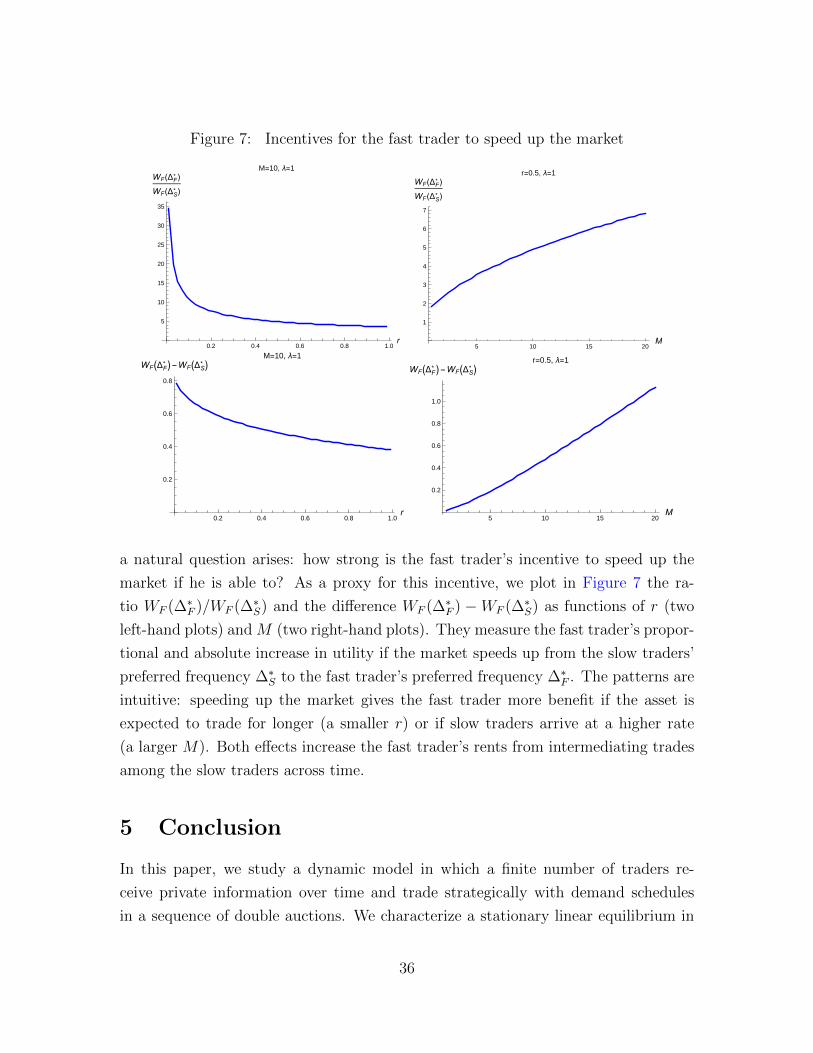
Figure 7: Incentives for the fast trader to speed up the market

0.2 0.4 0.6 0.8 1.0r

5

10

15

20

25

30

35

WF(ΔF* )

WF(ΔS* )

M=10, λ=1

5 10 15 20M

1

2

3

4

5

6

7

WF(ΔF* )

WF(ΔS* )

r=0.5, λ=1

0.2 0.4 0.6 0.8 1.0r

0.2

0.4

0.6

0.8

WFΔF* -WFΔS

* M=10, λ=1

5 10 15 20M

0.2

0.4

0.6

0.8

1.0

WFΔF* -WFΔS

* r=0.5, λ=1

a natural question arises: how strong is the fast trader’s incentive to speed up the

market if he is able to? As a proxy for this incentive, we plot in Figure 7 the ra-

tio WF (∆∗F )/WF (∆∗S) and the difference WF (∆∗F ) −WF (∆∗S) as functions of r (two

left-hand plots) and M (two right-hand plots). They measure the fast trader’s propor-

tional and absolute increase in utility if the market speeds up from the slow traders’

preferred frequency ∆∗S to the fast trader’s preferred frequency ∆∗F . The patterns are

intuitive: speeding up the market gives the fast trader more benefit if the asset is

expected to trade for longer (a smaller r) or if slow traders arrive at a higher rate

(a larger M). Both effects increase the fast trader’s rents from intermediating trades

among the slow traders across time.

5 Conclusion

In this paper, we study a dynamic model in which a finite number of traders re-

ceive private information over time and trade strategically with demand schedules

in a sequence of double auctions. We characterize a stationary linear equilibrium in

36

closed form. The equilibrium price aggregates a weighted sum of the common value

information and private values information, but the two components cannot be sep-

arated from the price. Due to imperfect competition, the equilibrium allocation is

not fully efficient, but it converges to the efficient allocation exponentially over time.

The presence of adverse selection—asymmetric information regarding the common-

value component of the asset—slows down this convergence speed. As the number

n of traders increases, the asymptotic convergence rate to efficiency is O(n−4/3) with

adverse selection and O(n−2) without adverse selection; the corresponding rates in

the continuous-time limit are O(n−2/3) and O(n−1), respectively.

We use this modeling framework to study the optimal trading frequency that

maximizes welfare. Trading frequency is measured as the number of double auctions

per unit of clock time. A higher trading frequency reduces the aggressiveness of de-

mand schedules, but allows more immediate reactions to new information. If traders

have homogeneous trading speed, slow trading tends to be optimal for scheduled in-

formation arrivals but fast trading tends to be optimal for stochastic information

arrivals. Moreover, the optimal trading frequency under stochastic information ar-

rivals is higher if the arrival rate of fundamental information is higher. If traders

have heterogeneous speeds (i.e., different frequencies of accessing the market), the

fast trader extracts rents by intermediating trades among slow traders across time.

As a result, the fast trader prefers the highest feasible trading frequency, whereas

slow traders tend to prefer a strictly lower frequency.

37

A List of Model Variables

Variable Explanation

Exogenous Variables

t Discrete trading period , t ∈ {0, 1, 2, 3, . . . }τ Continuous clock time, τ ∈ [0,∞)∆ Length of each trading periodT , r The clock time T of dividend payment has an exponential distribution with

intensity r > 0.{Tk}k∈{0,1,2,... } Times of shocks to the common dividend and private values

DTk The common dividend value immediately after the k-th shockσ2D Each dividend shock DTk −DTk−1

has the distribution N (0, σ2D).

Si,Tk Trader i’s signal of the k-th dividend shockσ2ε The noise in trader i’s dividend signal regarding the k-th dividend shock,

Si,Tk − (DTk −DTk−1), has the distribution N (0, σ2

ε ).wi,Tk Trader i’s private value for the asset immediately after the k-th shockσ2w Shocks to each trader i’s private value, wi,Tk −wi,Tk−1

, has the distributionN (0, σ2

w).λ Before the dividend is paid, the flow cost for holding asset position q is

0.5λq2 per unit of clock time for each trader.Z The total inventory held by all traders, Z ≡

∑1≤j≤n zj,0

γ Time interval of scheduled information arrivalsµ Intensity of stochastic information arrivals

Endogenous Variables

zi,t∆ Trader i’s inventory level right before the period-t double auctionxi,t∆(p) Trader i’s demand schedule in the period-t double auctionp∗t∆ The equilibrium price in period-t double auctionHi,t∆ Trader i’s history (information set) up to time t∆ but before the period-t

double auction, defined in (9)si,Tk Trader i’s total signal right after the k-th shock, defined in (14)vi,t∆ Trader i’s expected value for the asset, evaluated right after the period-t

double auction, given Hi,t∆ ∪ {Hj,t∆}j 6=iVi,t∆ The period-t ex post utility of trader i, evaluated right after the period-t

double auction, given Hi,t∆ ∪ {Hj,t∆}j 6=iχ, α Constants defined before Proposition 1

zci,(t+1)∆ The competitive allocation immediately after period-t auction

zei,τ The continuous-time version of competitive allocation

σ2z , σ

20 Constants defined in Equations (52) and (53)

W (∆) Welfare under homogeneous speed and trading interval ∆WF (∆) The fast trader’s welfare under heterogeneous speedWS(∆) Slow traders’ welfare under heterogeneous speed∆∗F , ∆∗S The fast and slow traders’ preferred frequencies under heterogeneous speed

38

B Proofs

B.1 Proof of Proposition 1

Before constructing the equilibrium, we first prove that our construction of totalsignal in (14) implies Equation (21).

Lemma 1. For any constant x, we have:

E[vi,Tk

∣∣∣Hi,Tk ∪{∑

j 6=i

(x∑k

l=0Sj,Tl + wj,Tk

)}](71)

=wi,Tk +1/(x2σ2

ε )

1/(x2σ2D) + 1/(x2σ2

ε ) + (n− 1)/(x2σ2ε + σ2

w)

k∑l=0

Si,Tl

+1/(x2σ2

ε + σ2w)

1/(x2σ2D) + 1/(x2σ2

ε ) + (n− 1)/(x2σ2ε + σ2

w)· 1

x

(∑j 6=i

(x

k∑l=0

Sj,Tl + wj,Tk

)).

Proof. DefineSi,Tl ≡ xSi,Tl + wi,Tl − wi,Tl−1

. (72)

By the projection theorem for multivariate normal distribution:

E[DTl −DTl−1

| Si,Tl ,∑

j 6=iSj,Tl

](73)

= (xσ2D, (n− 1)xσ2

D) ·(x2(σ2

D + σ2ε ) (n− 1)x2σ2

D

(n− 1)x2σ2D (n− 1)(x2(σ2

D + σ2ε ) + σ2

w) + (n− 1)(n− 2)x2σ2D

)−1

·(xSi,Tl ,

∑j 6=i

Sj,Tl

)′.

We compute:(x2(σ2

D + σ2ε ) (n− 1)x2σ2

D

(n− 1)x2σ2D (n− 1)(x2(σ2

D + σ2ε ) + σ2

w) + (n− 1)(n− 2)x2σ2D

)−1

=

((n− 1)(x2σ2

ε + σ2w) + (n− 1)2x2σ2

D −(n− 1)x2σ2D

−(n− 1)x2σ2D x2(σ2

D + σ2ε )

)· 1

(n− 1)x2(x2σ2ε + σ2

w)(σ2D + σ2

ε ) + (n− 1)2x4σ2Dσ

2ε

,

39

and

E[DTl −DTl−1

| Si,Tl ,∑

j 6=iSj,Tl

]=

(n− 1)x2σ2D(x2σ2

ε + σ2w)Si,Tl + (n− 1)x3σ2

Dσ2ε

∑j 6=i Sj,Tl

(n− 1)x2(x2σ2ε + σ2

w)(σ2D + σ2

ε ) + (n− 1)2x4σ2Dσ

2ε

=(1/x2σ2

ε )Si,Tl + (1/(x2σ2ε + σ2

w)) 1x

∑j 6=i Sj,Tl

1/(x2σ2ε ) + 1/(x2σ2

D) + (n− 1)/(x2σ2ε + σ2

w).

Summing the above equation across l ∈ {0, 1, . . . , k} and adding wi,Tk gives Equa-tion (71).

By Equation (71), we have

E[vi,Tk

∣∣∣Hi,Tk ∪{∑

j 6=i

(χ∑k

l=0Sj,Tl + wj,Tk

)}]=wi,Tk + χ

k∑l=0

Si,Tl +1/(χ2σ2

ε + σ2w)

1/(χ2σ2D) + 1/(χ2σ2

ε ) + (n− 1)/(χ2σ2ε + σ2

w)· 1

χ

(∑j 6=i

(χ

k∑l=0

Sj,Tl + wj,Tk

))

=αsi,Tk +1− αn− 1

∑j 6=i

sj,Tk ,

where in the second line we used the definition of χ in Equation (15), and in the thirdline we used the definition of si,Tk in (14), and the definition of α:

α ≡ 1

1 + (n−1)/(χ2σ2ε+σ2

w)

1/(χ2σ2D)+1/(χ2σ2

ε )+(n−1)/(χ2σ2ε+σ2

w)· 1χ

=χ2σ2

ε + σ2w

nχ2σ2ε + σ2

w

. (74)

We conjecture that traders use the following linear, symmetric and stationarystrategy:

xj,t∆(p; sj,t∆, zj,t∆) = asj,t∆ − bp+ dzj,t∆ + fZ. (75)

This conjecture implies the market-clearing prices of

p∗t∆ =a

nb

n∑j=1

sj,t∆ +d+ nf

nbZ. (76)

Fix a history Hi,t∆ and a realization of∑

j 6=i sj,t∆. We use the single-deviationprinciple to construct an equilibrium strategy (75): under the conjecture that othertraders j 6= i use strategy (75) in every period t′ ≥ t, and that trader i returns tostrategy (75) in period t′ ≥ t + 1, we verify that trader i has no incentive to deviatefrom strategy (75) in period t.22

22For a description of the single-deviation principle, also called “one-stage deviation principle”,

40

If trader i uses an alternative demand schedule in period t, he faces the resid-ual demand −

∑j 6=i xj,t∆(pt∆) and is effectively choosing a price pt∆ and getting

xi,t∆(pt∆) = −∑

j 6=i xj,t∆(pt∆). Therefore, by differentiating

E[Vi,t∆ | Hi,t∆ ∪

{∑j 6=i

sj,t∆

}]where Vi,t∆ is defined in (12), with respect to pt∆ and evaluating it at pt∆ = p∗t∆ in(76), we obtain the following first order condition in period t of trader i:

E

[(n− 1)b ·

((1− e−r∆)

∞∑k=0

e−rk∆∂(zi,(t+k)∆ + xi,(t+k)∆)

∂xi,t∆

(vi,(t+k)∆ −

λ

r(zi,(t+k)∆ + xi,(t+k)∆)

)

−∞∑k=0

e−rk∆∂xi,t∆∂xi,0

p∗t∆

)−∞∑k=0

e−rk∆ xi,(t+k)∆

∂p∗(t+k)∆

∂pt∆

∣∣∣∣∣ Hi,t∆ ∪{∑

j 6=isj,t∆

}]= 0,

(77)

where we write xi,(t+k)∆ = xi,(t+k)∆(p∗(t+k)∆; si,(t+k)∆, zi,(t+k)∆) for the strategy xi,(t+k)∆( · )defined in (75), and by definition zi,(t+k+1)∆ = zi,(t+k)∆ + xi,(t+k)∆.

Since all traders follow the conjectured strategy in (75) from period t + 1 andonwards, we have the following evolution of inventories: for any k ≥ 1,

zi,(t+k)∆ + xi,(t+k)∆ =asi,(t+k)∆ − bp∗(t+k)∆ + fZ + (1 + d)zi,(t+k)∆ (78)

=(asi,(t+k)∆ − bp∗(t+k)∆ + fZ) + (1 + d)(asi,(t+k−1)∆ − bp∗(t+k−1)∆ + fZ)

+ · · ·+ (1 + d)k−1(asi,(t+1)∆ − bp∗(t+1)∆ + fZ) + (1 + d)k(xi,t∆ + zi,t∆).

The evolution of prices and inventories, given by Equations (76) and (78), revealsthat by changing the demand or price in period t, trader i has the following effectson inventories and prices in period t+ k, k ≥ 1:

∂(zi,(t+k)∆ + xi,(t+k)∆)

∂xi,t∆= (1 + d)k, (79)

∂xi,(t+k)∆

∂xi,t∆= (1 + d)k−1d, (80)

∂p∗(t+k)∆

∂pt∆=∂p∗(t+k)∆

∂xi,t∆= 0. (81)

As we verify later, the equilibrium value of d satisfies −1 < d < 0, so the partialderivatives (79) and (80) converge.

see Theorem 4.1 and 4.2 of Fudenberg and Tirole (1991). We can apply their Theorem 4.2 becausethe payoff function in our model, which takes the form of a “discounted” sum of period-by-periodpayoffs, satisfies the required “continuity at infinity” condition.

41

The first order condition in (77) simplifies to:

E

[(n− 1)b

((1− e−r∆)

∞∑k=0

e−rk∆(1 + d)k(vi,(t+k)∆ −

λ

r(zi,(t+k)∆ + xi,(t+k)∆)

)

− p∗t∆ −∞∑k=1

e−rk∆(1 + d)k−1d p∗(t+k)∆

)− xi,t∆

∣∣∣∣∣ Hi,t∆ ∪{∑

j 6=isj,t∆

}]= 0,

(82)

where we have (cf. Lemma 1, Equations (76) and (78)):

E[p∗i,(t+k)∆ | Hi,t∆ ∪ {sj,τ}j 6=i,0≤τ≤t∆] = p∗t∆, (83)

E[vi,(t+k)∆ | Hi,t∆ ∪ {sj,τ}j 6=i,0≤τ≤t∆] = E[vi,t∆ | Hi,t∆ ∪

{∑j 6=i

sj,t∆

}]= αsi,t∆ +

1− αn− 1

∑j 6=i

sj,t∆, (84)

E[zi,(t+k)∆ + xi,(t+k)∆ | Hi,t∆ ∪ {sj,τ}j 6=i,0≤τ≤t∆]

= (asi,t∆ − bp∗t∆ + fZ)

(1

−d− (1 + d)k

−d

)+ (1 + d)k(xi,t∆ + zi,t∆). (85)

Substituting Equations (76), (83), (84) and (85) into the first-order condition (82)and using the notation st∆ =

∑1≤j≤n sj,t∆/n, we get:

(n− 1)b(1− e−r∆)

[1

1− e−r∆(1 + d)

(αsi,t∆ +

1− αn− 1

∑j 6=i

sj,t∆ −(a

bst∆ +

d+ nf

nbZ

))

−∞∑k=0

λ

re−rk∆(1 + d)k

(1

−d− (1 + d)k

−d

)(asi,t∆ − b

(a

bst∆ +

d+ nf

nbZ

)+ fZ

)

− λ

(1− e−r∆(1 + d)2)r(xi,t∆ + zi,t∆)

]− xi,t∆ = 0. (86)

42

Rearranging the terms gives:(1 +

(n− 1)b(1− e−r∆)λ

(1− e−r∆(1 + d)2)r

)xi,t∆ (87)

= (n− 1)b(1− e−r∆)

[1

1− e−r∆(1 + d)

(nα− 1

n− 1si,t∆ +

n− nαn− 1

st∆ −a

bst∆

)− λe−r∆(1 + d)

r(1− (1 + d)e−r∆)(1− (1 + d)2e−r∆)a(si,t∆ − st∆)

− λ

(1− e−r∆(1 + d)2)rzi,t∆

−(

1

1− e−r∆(1 + d)

(d+ nf

nb+

λ

rn

)− λ

(1− (1 + d)2e−r∆)nr

)Z

].

On the other hand, substituting Equation (76) into the conjectured strategy (75)gives:

xi,t∆ = a(si,0 − s0) + dzi,0 −d

nZ. (88)

We match the coefficients in Equation (88) with those in Equation (87). First of all,we clearly have

a = b. (89)

We also obtain two equations for b and d:(1 +

(n− 1)b(1− e−r∆)λ

(1− e−r∆(1 + d)2)r

)=

(1− e−r∆)(nα− 1)

1− e−r∆(1 + d)− (n− 1)b(1− e−r∆)e−r∆(1 + d)λ

(1− (1 + d)e−r∆)(1− (1 + d)2e−r∆)r,(

1 +(n− 1)b(1− e−r∆)λ

(1− e−r∆(1 + d)2)r

)d = −(n− 1)b(1− e−r∆)λ

(1− e−r∆(1 + d)2)r. (90)

There are two solutions to the above system of equations. One of them leads tounbounded inventories, so we drop it.23 The other solution leads to converging in-ventories and is given by

b =(nα− 1)r

2(n− 1)e−r∆λ

((nα− 1)(1− e−r∆) + 2e−r∆ −

√(nα− 1)2(1− e−r∆)2 + 4e−r∆

),

(91)

d = − 1

2e−r∆

((nα− 1)(1− e−r∆) + 2e−r∆ −

√(nα− 1)2(1− e−r∆)2 + 4e−r∆

).

(92)

23This dropped solution to (90) has the property of (1+d)e−r∆ < −1, which leads to an unboundedpath of inventories (cf. Equation (78)) and utilities.

43

Lastly, matching the coefficient of Z gives:

f = −dn− bλ

nr. (93)

Under the condition nα > 2, we can show that b > 0 and −1 < d < 0, thatis, the demand schedule is downward-sloping in price and the inventories evolutions(79)–(80) converge.

By Equation (15), the condition nα > 2 is equivalent to the condition

χ2 <(n− 2)σ2

w

nσ2ε

(94)

which is equivalent to the following condition on the fundamentals:

1

n/2 + σ2ε/σ

2D

<

√n− 2

n

σwσε. (95)

Finally, we verify the second-order condition. Under the linear strategy in (75)with b > 0, differentiating the first-order condition (77) with respect to p0 gives

(n− 1)b(1− e−r∆)

(−λr

(n− 1)b∞∑k=0

e−rk∆(1 + d)2k − 1

)− (n− 1)b < 0. (96)

This completes the construction of a perfect Bayesian equilibrium.

B.2 Proof of Proposition 2

Suppose that every trader i use the strategy:

xi,t∆(p) =∑Tl≤t∆

alSi,Tl + awwi,t∆ − bp+ dzi,t∆ + f, (97)

where {al}l≥0, aw, b, d and f are constants. We show that for everyone using (97) tobe a perfect Bayesian equilibrium (PBE), the constants must be the ones given byProposition 1. We divide our arguments into two steps.

Step 1. Define xl ≡ al/aw. 24 As a first step, we show that if (97) is a symmetricPBE, then we must have xl = χ for every l, where χ is defined in Equation (15).

Suppose that (t − 1)∆ ∈ [Tk′ , Tk′+1) and t∆ ∈ [Tk, Tk+1), so there are k − k′ ≥ 1dividend shocks between time (t − 1)∆ and time t∆. 25 Without loss of generality,assume k′ = 0. Since all other traders j 6= i are using strategy (97), by computing

24Clearly, we cannot have aw = 0, since players use their private values in any equilibrium.25In period t = 0, we take DT−1 = wi,T−1 = 0.

44

the difference p∗t∆ − p∗(t−1)∆, trader i can infer from the period-t price the value of

∑j 6=i

k∑l=1

xlSj,Tl + wj,Tl − wj,Tl−1.

By the projection theorem for normal distribution, we have

E[DTk −DT0 | Hi,t∆ ∪

{∑j 6=i

∑Tl≤t∆

xlSj,Tl + wj,Tl − wj,Tl−1

}](98)

=E[DTk −DT0 | {Si,Tl}kl=1 ∪

{∑j 6=i

∑k

l=1xlSj,Tl + wj,Tl − wj,Tl−1

}]= u Σ−1 ·

(Si,T1 , . . . , Si,Tk ,

∑j 6=i

∑k

l=1xlSj,Tl + wj,Tl − wj,Tl−1

)′,

where Σ is the covariance matrix of(Si,T1 , . . . , Si,Tk ,

∑j 6=i∑k

l=1 xlSj,Tl + wj,Tl − wj,Tl−1

):

for 1 ≤ l ≤ k + 1 and 1 ≤ m ≤ k + 1,

Σl,m =

σ2D + σ2

ε 1 ≤ l = m ≤ k

0 1 ≤ l 6= m ≤ k

(n− 1)(∑k

l′=1 x2l′)(σ

2D + σ2

ε ) + (n− 1)kσ2w l = m = k + 1

+(n− 1)(n− 2)∑k

l′=1 x2l′σ

2D

(n− 1)xlσ2D 1 ≤ l ≤ k,m = k + 1

, (99)

and Σk+1,l = Σl,k+1. And u is a row vector of covariances between(Si,T1 , . . . , Si,Tk ,

∑j 6=i∑k

l=1 xlSj,Tl + wj,Tl − wj,Tl−1

)and DTk −DT0 :

u = (σ2D, . . . , σ

2D, (n− 1)

∑k

l=1xlσ

2D). (100)

Therefore, we have

E[vi,t∆ | Hi,t∆ ∪

{∑j 6=i

∑Tl≤t∆

xlSj,Tl + wj,Tl − wj,Tl−1

}](101)

=wi,Tk + E[DT0 | {Si,T0} ∪{∑

j 6=ix0Sj,T0 + wj,0

}]

+ u Σ−1 ·(Si,T1 , . . . , Si,Tk ,

∑j 6=i

∑k

l=1xlSj,Tl + wj,Tl − wj,Tl−1

)′.

Since we look for a symmetric equilibrium in which everyone plays (97), trader i’sconditional value in (101) must place a weight of xl on Si,Tl , 1 ≤ l ≤ k, which impliesthat

u Σ−1 = x, (102)

45

where x = (x1, . . . , xk, y) and y is an arbitrary number. Clearly, Equation (102) isequivalent to

u = x Σ,

which implies (from the first k entries of the row vector)

σ2D = xl(σ

2D + σ2

ε ) + y(n− 1)xlσ2D, 1 ≤ l ≤ k,

i.e.,

x1 = · · · = xk =σ2D

σ2D + σ2

ε + y(n− 1)σ2D

.

Now define x ≡ x1 = · · · = xk. Applying Lemma 1 to the conditional value in(101) implies that for the conditional value in (101) to place a weight of x on Si,Tl ,1 ≤ l ≤ k, we must have x = χ.

Step 2. Given Step 1, we can rewrite the strategy (97) as

xi,t∆(p) = aw · α si,t∆ − bp+ dzi,t∆ + f, (103)

where si,t∆ is the total signal defined in (14) and α is defined in (16). The equilibriumconstruction in Section B.1 then uniquely determines the values of aw, b, d and f .This concludes the proof of Proposition 2.

B.3 Proof of Proposition 3

We first prove the convergence to competitive allocation. Conditional on the totalsignals staying the same from period t to t, the efficient allocation in each of theseperiods is also the same and is given by

zci,(t+1)∆ =r(nα− 1)

λ(n− 1)

(si,t∆ −

1

n

n∑j=1

sj,t∆

)+

1

nZ. (104)

We rewrite the perfect Bayesian equilibrium strategy (18) as

xi,t∆(p; si,t∆, zi,t∆) = asi,t∆ − bp+ dzi,t∆ + fZ. (105)

It is easy to verify that at the competitive allocation zci,(t+1)∆, trader i trades zerounit in equilibrium:

xi,t∆(p∗t∆; si,t∆, zci,(t+1)∆) = 0; (106)

one way to see this is to note that the perfect Bayesian equilibrium strategy is ascaled version of the competitive equilibrium strategy (Equation (32)).

46

That is, for every i ∈ {1, 2, . . . , n},

zci,(t+1)∆ =asi,t∆ − bp∗i,t∆ + fZ

−d. (107)

By definition, we have

z∗i,(t+1)∆ = z∗i,t∆ + xi,t∆(p∗i,t∆; si,t∆, z∗i,t∆)

= asi,t∆ − bp∗i,t∆ + (1 + d)z∗i,t∆ + fZ

= (−d)zci,(t+1)∆ + (1 + d)z∗i,t∆,

where the last equality follows from (107). This proves (34) for t = t. The case oft > t follows by induction.

Now we prove the comparative statics. We write

1 + d =1

2e−r∆

(√(nα− 1)2(1− e−r∆)2 + 4e−r∆ − (nα− 1)(1− e−r∆)

), (108)

andη ≡ nα− 1. (109)

We first note that ∂(1+d)∂η

< 0.

1. The comparative statics with respect to r follow by straightforward calculationsshowing that ∂(1+d)

∂r< 0.

2. As σ2D increases, the left-hand side of Equation (15) increases, and hence the

solution χ to (15) increases, which means that nα decreases because according to

Equation (16) nα is a decreasing function of χ2. Thus, ∂η∂σ2D< 0, and ∂(1+d)

∂σ2D

> 0.

3. As σ2w increases, the left-hand side of Equation (15) increases, and hence the

solution χ to (15) increases; by (15) this means that σ2w/χ

2 must increase aswell. Thus, nα increases because according to Equation (16) nα is an increasing

function of σ2w/χ

2. Hence, ∂η∂σ2w> 0 and ∂(1+d)

∂σ2w

< 0.

4. We can rewrite Equation (15) as

11α

+ σ2ε

σ2D

= χ, (110)

and Equation (16) as

χ =

√1− αnα− 1

σwσε, (111)

47

and hence1

nη+1

+ σ2ε

σ2D

=

√n− η − 1

nη

σwσε. (112)

From Equation (112) is it straightforward to show that η must increase with n.Thus, 1 + d decreases in n.

5. For the comparative statics with respect to ∆, we find that

∂(log(1 + d)/∆)

∂∆= − 1

∆2

(r∆

η√η2(er∆ − 1)2 + 4er∆ − η2(er∆ − 1)− 2√

η2(1− e−r∆)2 + 4e−r∆(√

η2(er∆ − 1)2 + 4er∆ − η(er∆ − 1))

+ log

(1

2

(√η2(er∆ − 1)2 + 4er∆ − η(er∆ − 1)

)))> 0.

B.4 Proofs of Propositions 5, 6, 7 and 8

We first establish some general properties of the equilibrium welfare, before specializ-ing to the rate that inefficiency vanishes as n→∞ (Section B.4.1), and to the optimaltrading frequency given scheduled (Section B.4.2 and Section B.4.3) and stochastic(Section B.4.4) arrivals of new information.

The following lemma relates the amount of inefficiency associated with an inven-tory allocation to the square distance between that allocation and the competitiveallocation:

Lemma 2. Let {zei } be the competitive allocation given the total signals {si}:

{zei } = argmax{z′i}

n∑i=1

((αsi +

1− αn− 1

∑j 6=i

sj

)(z′i)−

λ

2r(z′i)

2

)subject to:

n∑i=1

z′i = Z.

For any profile of inventories (z1, z2, . . . , zn) satisfying∑n

i=1 zi = Z, we have:

n∑i=1

((αsi +

1− αn− 1

∑j 6=i

sj

)zei −

λ

2(zei )

2

)−

n∑i=1

((αsi +

1− αn− 1

∑j 6=i

sj

)zi −

λ

2(zi)

2

)

=λ

2r

n∑i=1

(zi − zei )2. (113)

Proof. First, by the definition of competitive allocation, we have(αsi +

1− αn− 1

∑j 6=i

sj

)− λzei = ν (114)

48

for every i, where ν is the Lagrange multiplier for the constraint∑n

i=1 zei = Z in the

maximization problem of {zei }.Since (zi)

2 = (zei )2 + 2zei (zi − zei ) + (zi − zei )2, we have:

n∑i=1

((αsi +

1− αn− 1

∑j 6=i

sj

)zi −

λ

2r(zi)

2

)(115)

=n∑i=1

((αsi +

1− αn− 1

∑j 6=i

sj

)zei −

λ

2r(zei )

2

)+

n∑i=1

((αsi +

1− αn− 1

∑j 6=i

sj

)− λ

rzei

)(zi − zei )

− λ

2r

n∑i=1

(zi − zei )2.

The middle term in the right-hand side of (115) is zero because of (114) and of∑ni=1(zi − zei ) = Z − Z = 0. This proves the lemma.

By Lemma 2 we write W (∆) as:

W (∆) = E

[∫ ∞τ=0

re−rτn∑i=1

(vi,τz

ei,τ −

λ

2r(zei,τ )

2

)dτ

]−X(∆), (116)

where

X(∆) = E

[∫ ∞τ=0

re−rτλ

2r

n∑i=1

(zei,τ − z∗i,τ )2 dτ

](117)

is the amount of inefficiency associated with the equilibrium path of inventories. Sincethe first term on the right-hand side of (116) is the welfare of competitive allocationin continuous time and is hence independent of ∆, the optimal trading frequency isdetermined by the comparative statics of X(∆) with respect to ∆.

Lemma 3. Suppose that τ ∈ (t∆, (t+ 1)∆). Then we have

E[(z∗i,τ − zei,τ )2] = E[(z∗i,(t+1)∆ − zei,t∆)2] + E[(zei,t∆ − zei,τ )2]. (118)

Proof. Recall that z∗i,τ = z∗i,(t+1)∆ for τ ∈ (t∆, (t + 1)∆) because trading does not

happen in (t∆, (t+ 1)∆). Thus, we can rewrite, for any τ ∈ (t∆, (t+ 1)∆),

E[(z∗i,τ−zei,τ )2] = E[(z∗i,(t+1)∆−zei,t∆)2]+E[(zei,t∆−zei,τ )2]+E[2(z∗i,(t+1)∆−zei,t∆)(zei,t∆−zei,τ )].(119)

Since z∗i,(t+1)∆ is measurable with respect to {Hj,t∆}1≤j≤n, τ > t∆, and {zei,τ ′}τ ′≥0

is a martingale, we have E[(z∗i,(t+1)∆ − zei,t∆)(zei,t∆ − zei,τ )] = 0 by the law of iteratedexpectations.

49

By Lemma 3, we can further decompose X(∆) into two terms:

X(∆) = X1(∆) +X2(∆), (120)

where

X1(∆) = (1− e−r∆) · λ2r

n∑i=1

∞∑t=0

e−rt∆E[(z∗i,(t+1)∆ − zei,t∆)2] (121)

and

X2(∆) =λ

2r

n∑i=1

∞∑t=0

∫ (t+1)∆

τ=t∆

re−rτE[(zei,t∆ − zei,τ )2] dτ. (122)

The expression X2(∆) is purely in terms of the competitive inventories zei,t∆ andis relatively easy to analyze because zei,τ depends only on the total signals at timeτ . In contrast, X1(∆) is a function of the equilibrium inventories z∗i,τ which dependson all total signals on and before time τ . The next lemma simplifies the equilibriuminventory terms in X1(∆).

Lemma 4.

E[(z∗i,(t+1)∆−zei,t∆)2] = (1+d)2(t+1)E[(z∗i,0−zei,0)2]+t−1∑t′=0

(1+d)2(t−t′)E[(zei,(t′+1)∆−zei,t′∆)2]

(123)

Proof. From Proposition 3 (where zei,t∆ = zci,(t+1)∆), we have

z∗i,(t+1)∆ − zei,t∆ = (1 + d)(z∗i,t∆ − zei,t∆). (124)

Therefore,

E[(z∗i,(t+1)∆ − zei,t∆)2] = (1 + d)2E[(z∗i,t∆ − zei,t∆)2]

= (1 + d)2E[(z∗i,t∆ − zei,(t−1)∆)2] + (1 + d)2E[(zei,t∆ − zei,(t−1)∆)2]

− 2(1 + d)2E[(z∗i,t∆ − zei,(t−1)∆)(zei,t∆ − zei,(t−1)∆)]. (125)

Because z∗i,t∆ is measurable with respect to {Hj,(t−1)∆}1≤j≤n and {zei,τ}τ≥0 is a mar-tingale, E[(z∗i,t∆ − zei,(t−1)∆)(zei,t∆ − zei,(t−1)∆)] = 0 by the law of iterated expectations.The rest follows by induction.

Finally, Lemma 5 expresses X1(∆) in terms of the competitive inventories, similarto X2(∆).

Lemma 5.

X1(∆) =λ(1 + d)

2r(nα− 1)

(n∑i=1

E[(zi,0 − zei,0)2] +n∑i=1

∞∑t=0

e−r(t+1)∆E[(zei,(t+1)∆ − zei,t∆)2]

).

(126)

50

Proof. By Lemma 4, we have

X1(∆) (127)

=λ(1− e−r∆)

2r

n∑i=1

∞∑t=0

e−rt∆

((1 + d)2(t+1)E[(z∗i,0 − zei,0)2] +

t−1∑t′=0

(1 + d)2(t−t′)E[(zei,(t′+1)∆ − zei,t′∆)2]

)

=λ

2r

(1− e−r∆)(1 + d)2

1− (1 + d)2e−r∆

n∑i=1

E[(z∗i,0 − zei,0)2]

+1− e−r∆

r

λ

2

n∑i=1

∞∑t′=0

E[(zei,(t′+1)∆ − zei,t′∆)2]∞∑

t=t′+1

e−rt∆(1 + d)2(t−t′)

=λ

2r

(1− e−r∆)(1 + d)2

1− (1 + d)2e−r∆

n∑i=1

E[(z∗i,0 − zei,0)2]

+λ

2r

(1− e−r∆)(1 + d)2

1− (1 + d)2e−r∆

n∑i=1

∞∑t′=0

E[(zei,(t′+1)∆ − zei,t′∆)2]e−r(t′+1)∆.

We can simplify the constant in the above equations by a direct calculation:

e−r∆(1 + d)2 (128)

=2(nα− 1)2(1− e−r∆)2 + 4e−r∆ − 2(nα− 1)(1− e−r∆)

√(nα− 1)2(1− e−r∆)2 + 4e−r∆

4e−r∆

= 1− (nα− 1)(1− e−r∆)(1 + d),

which implies:(1− e−r∆)(1 + d)2

1− (1 + d)2e−r∆=

1 + d

nα− 1. (129)

Finally, by construction: z∗i,0 = zi,0 for every bidder i.

B.4.1 Proofs of Proposition 5

Suppose that T0 = 0 and {Tk}k≥1 is a homogeneous Poisson process with intensityµ > 0. (The proof for scheduled information arrivals Tk = kγ is analogous.)

Lemma 5 then implies that

X(∆)

n=λ(1 + d(∆))

2r(nα− 1)·

(∑ni=1 E[(zi,0 − zei,0)2]

n+e−r∆µ∆

1− e−r∆

∑ni=1 E[(zei,Tk − z

ei,Tk−1

)2]

n

),

(130)where for any k ≥ 1,∑n

i=1 E[(zei,Tk − zei,Tk−1

)2]

n=

(r(nα− 1)

λ(n− 1)

)2(n− 1)(χ2(σ2

D + σ2ε ) + σ2

w)

nα2, (131)

51

by Equation (52).Equation (131) tends to a constant as n → ∞ (since χ → 0 as n → ∞), and

lim∆→0e−r∆µ∆1−e−r∆ = µ

r. By assumption,

∑ni=1 E[(zi,0 − zei,0)2]/n is bounded as n → ∞.

Thus, for limn→∞X1(∆)/n it suffices to analyze

1 + d(∆)

nα− 1=

1

2e−r∆

(√(1− e−r∆)2 +

4e−r∆

(nα− 1)2− (1− e−r∆)

). (132)

Suppose that σ2D > 0 and ∆ > 0. Equation (112) (where η ≡ nα− 1) implies that

nα = O(n2/3) as n→∞. To see this, first note that η →∞ and η/n→ 0 as n→∞,for otherwise the left-hand side and right-hand side of Equation (112) cannot match.Suppose that as n becomes large, η = O(ny) for some y < 1. The left-hand sideof Equation (112) is of order O(ny−1), and the right-hand side is of order O(n−y/2).Thus, y = 2/3. It is straightforward to calculate that, as n becomes large,

O

(1 + d(∆)

nα− 1

)= O((nα− 1)−2) = O(n−4/3).

But if we first take the limit ∆→ 0, we clearly have

lim∆→0

1 + d(∆)

nα− 1=

1

nα− 1= O(n−2/3), as n becomes large.

If σ2D = 0, then nα = n. The same calculation as above shows that X(∆)/n is of

order O(n−2) for a fixed ∆ > 0 but of order O(n−1) if we first take the limit ∆→ 0.

B.4.2 Proof of Proposition 6

For any τ > 0, we let t(τ) = min{t ≥ 0 : t ∈ Z, t∆ ≥ τ}. That is, if new signalsarrive at the clock time τ , then t(τ)∆ is the clock time of the next trading period(including time τ).

For any ∆ ≤ γ, by the assumption of Proposition 6 there is at most one newsignal profile arrival in each interval [t∆, (t+ 1)∆). Thus, we only need to count thechanges in competitive allocation between period t((k − 1)γ) and t(kγ), for k ∈ Z+.

52

Using this fact, we can rewrite X1(∆) and X2(∆) as:

X1(∆) =λ(1 + d)

2r(nα− 1)

(n∑i=1

E[(zi,0 − zei,0)2] +n∑i=1

∞∑k=1

e−rt(kγ)∆E[(zei,kγ − zei,(k−1)γ)2]

)

=λ(1 + d)

2r(nα− 1)

(n∑i=1

E[(zi,0 − zei,0)2] +n∑i=1

∞∑k=1

e−rkγE[(zei,kγ − zei,(k−1)γ)2]

)

− λ(1 + d)

2r(nα− 1)

n∑i=1

∞∑k=1

(e−rkγ − e−rt(kγ)∆)E[(zei,kγ − zei,(k−1)γ)2]. (133)

and

X2(∆) =λ

2r

n∑i=1

∞∑t=0

∫ (t+1)∆

τ=t∆

re−rτE[(zei,t∆ − zei,τ )2] dτ (134)

=λ

2r

n∑i=1

∞∑k=1

(e−rkγ − e−rt(kγ)∆)E[(zei,kγ − zei,(k−1)γ)2].

Note that all the expectations in the expressions of X1(∆) and X2(∆) do notdepend on ∆. To make clear the dependence of d on ∆, we now write d = d(∆).Since (1 + d(∆))/(nα− 1) < 1, we have for any ∆ < γ:

X(∆) = X1(∆) +X2(∆) (135)

>λ(1 + d(∆))

2r(nα− 1)

(n∑i=1

E[(zi,0 − zei,0)2] +n∑i=1

∞∑k=1

e−rkγE[(zei,kγ − zei,(k−1)γ)2]

)

>λ(1 + d(γ))

2r(nα− 1)

(n∑i=1

E[(zi,0 − zei,0)2] +n∑i=1

∞∑k=1

e−rkγE[(zei,kγ − zei,(k−1)γ)2]

)= X(γ),

where the last inequality holds because d(∆) decreases with ∆ (which can be verifiedby taking derivative the d′(∆)) and where the last equality holds because t(kγ)∆ =kγ if γ = ∆. Therefore, we have W (∆) < W (γ) for any ∆ < γ. This provesProposition 6.

Notice that for this lower bound of ∆∗ ≥ γ we make no use of the assumptionthat E[(zei,kγ − zei,(k−1)γ)

2] is a constant independent of k.

53

B.4.3 Proof of Proposition 7

If ∆ = lγ, where l ≥ 1 is an integer, we have:

X1(lγ) =λ(1 + d(lγ))

2r(nα− 1)

(σ2

0 +∞∑t=0

e−r(t+1)lγlσ2z

)=λ(1 + d(lγ))

2r(nα− 1)

(σ2

0 +e−rlγ

1− e−rlγlσ2z

).

(136)

X2(lγ) =λ

2r

1

1− e−rlγ((e−γr − e−2γr) + 2(e−2γr − e−3γr) + · · ·+ (l − 1)(e−(l−1)γr − e−lγr)

)σ2z

=λ

2r

1

1− e−rlγ(e−γr + e−2γr + e−3γr + · · ·+ e−(l−1)γr − (l − 1)e−lγr

)σ2z

=λ

2r

1

1− e−rlγ

(1− e−rlγ

1− e−γr− 1− (l − 1)e−rlγ

)σ2z

=λ

2r

(1

1− e−γr− 1− l e−rlγ

1− e−rlγ

)σ2z . (137)

Hence, if ∆ = lγ, l ∈ Z+, we have:

X(lγ) =λ(1 + d(lγ))

2r(nα− 1)σ2

0 −λ

2r

(1− 1 + d(lγ)

nα− 1

)le−rlγ

1− e−rlγσ2z +

λe−γr

2r(1− e−γr)σ2z .

(138)

By taking derivative, we can show that the function (involved in the first term in(138))

1 + d(∆)

nα− 1=

1

2e−r∆

(√(1− e−r∆)2 +

4e−r∆

(nα− 1)2− (1− e−r∆)

)is strictly decreasing in ∆. And since(

1− 1 + d(∆)

nα− 1

)∆e−r∆

1− e−r∆=

(nα− 1)(1 + e−r∆)−√

(nα− 1)2(1− e−r∆)2 + 4e−r∆

2(nα− 1)e−r∆/2· ∆e−r∆/2

1− e−r∆,

and both terms on the right-hand side are strictly decreasing in ∆ (easily verifiedwith derivatives), the above function (involved in the second term in (138)) is alsostrictly decreasing in ∆.

Without loss of generality, suppose that σ2z = 1. The above discussion implies

that the function X(lγ) satisfies strictly decreasing difference condition with respectto variables l and σ2

0 = σ20/σ

2z :

∂2X(lγ)

∂l ∂σ20

< 0. (139)

Therefore, by a well-known result in monotone comparative statics (Theorem 5 in

54

Milgrom and Shannon (1994)), l∗ that minimizes X(lγ) is weakly increasing withσ2

0 = σ20/σ

2z . As σ2

0/σ2z → 0, the second term in (138) dominates, and hence X(lγ) is

minimized at l∗ = ∞. As σ20/σ

2z → ∞, the first term in (138) dominates, and hence

X(lγ) is minimized at l∗ = 1.Finally, as n tends to infinity, the proof of Proposition 5 implies that nα tends

to infinity as well. As nα → ∞, (1 + d(lγ))/(nα − 1) → 0 for every l ∈ Z+, andby assumption σ2

0/σ2z remains bounded, so the second term in (138) dominates, and

hence X(lγ) is minimized at l∗ = 1.

B.4.4 Proof of Proposition 8

Since dividend shocks arrive according to a Poisson process with the intensity µ, wehave

n∑i=1

E[(zei,τ − zei,t∆)2] = (τ − t∆)µσ2z , τ ∈ [t∆, (t+ 1)∆), (140)

n∑i=1

E[(zei,(t+1)∆ − zei,t∆)2] = ∆µσ2z . (141)

Substituting the above two expressions into (122) and (126), we have:

X1(∆) =λ(1 + d)

2r(nα− 1)

(σ2

0 +∞∑t=0

e−r(t+1)∆∆µσ2z

)(142)

=λ(1 + d)

2r(nα− 1)

(σ2

0 +∆e−r∆

1− e−r∆µσ2

z

)and

X2(∆) =λ

2r

∞∑t=0

e−rt∆∫ ∆

τ=0

re−rττµσ2z dτ = − λ

2r

∆e−r∆

1− e−r∆µσ2

z +λ

2r2µσ2

z . (143)

Therefore,

X(∆) =λ(1 + d)

2r(nα− 1)σ2

0 −λ

2r

(1− 1 + d

nα− 1

)∆e−r∆

1− e−r∆µσ2

z +λ

2r2µσ2

z . (144)

We note that the above is the same expression as Equation (138) in the proof ofProposition 7; therefore, the proof of Proposition 8 is the same as that of Proposition 7with the modification that here ∆ is not restricted to integer multiple of γ, and hencethe comparative statics is strict.

55

B.5 Proof of Proposition 9

We have derived the slow traders’ equilibrium strategies in the text following Propo-sition 9, so here we focus on characterizing the fast trader’s equilibrium strategy.

We conjecture that the fast trader uses the strategy

xF,t∆(p; zF,t∆) = −bFp+ dF zF,t∆. (145)

Without loss of generality let us specialize to period 1 with an arbitrary inventoryzF,∆. Assuming that the fast trader uses strategy (145) from period 2 and onwards,and that the slow traders use their equilibrium strategy (59) in every period, we willconstruct strategy (145) such that the fast trader has no incentive to deviate fromstrategy (145) in period 1. By the single deviation principle, this gives the equilibriumstrategy of the fast trader.

Under our assumption about the traders’ strategies from period 2 and onwards,we have for t ≥ 1:

p∗(t+1)∆ =1

bF + nSbS

(nS∑j=1

bSwj,(t+1)∆ + dF zF,(t+1)∆

), (146)

and

zF,(t+2)∆ = zF,(t+1)∆ + xF,(t+1)∆

= zF,(t+1)∆ − bFp∗(t+1)∆ + dF zF,(t+1)∆

= zF,(t+1)∆ +−bF

bF + nSbS

nS∑j=1

bSwj,(t+1)∆ +−bF

bF + nSbSdF zF,(t+1)∆ + dF zF,(t+1)∆

=−bF

bF + nSbS

nS∑j=1

bSwj,(t+1)∆ +

(1 +

nSbSbF + nSbS

dF

)zF,(t+1)∆. (147)

Therefore, the fast trader in period 1 has the following effect on the future prices andinventories:

∂(zF,(t+1)∆ + xF,(t+1)∆)

∂xF,∆=

(1 +

nSbSbF + nSbS

dF

)t, (148)

∂xF,(t+1)∆

∂xF,∆=

(1 +

nSbSbF + nSbS

dF

)t−1nSbS

bF + nSbSdF , (149)

∂p∗(t+1)∆

∂xF,∆=

(1 +

nSbSbF + nSbS

dF

)t−1dF

bF + nSbS. (150)

56

The fast trader’s first order condition at period 1 is:

−xF,∆ + nSbS

[1− e−r∆

r

∞∑t=0

e−rt∆E[−λ(zF,(t+1)∆ + xF,(t+1)∆)

∂(zF,(t+1)∆ + xF,(t+1)∆)

∂xF,∆| zF,∆, xF,∆

](151)

− p∗∆ −∞∑t=1

e−rt∆E[∂xF,(t+1)∆

∂xF,∆p∗(t+1)∆ | zF,∆, xF,∆

]

−∞∑t=1

e−rt∆E[∂p∗(t+1)∆

∂xF,∆xF,(t+1)∆ | zF,∆, xF,∆

]]= 0,

i.e.,

−xF,∆ + nSbS

[1− e−r∆

r

∞∑t=0

e−rt∆(

1 +nSbS

bF + nSbSdF

)t(−λE[zF,(t+1)∆ + xF,(t+1)∆ | zF,∆, xF,∆])

(152)

−p∗∆ −∞∑t=1

e−rt∆(

1 +nSbS

bF + nSbSdF

)t−1nSbS

bF + nSbSdFE[p∗(t+1)∆ | zF,∆, xF,∆]

−∞∑t=1

e−rt∆(

1 +nSbS

bF + nSbSdF

)t−1dF

bF + nSbSE[xF,(t+1)∆ | zF,∆, xF,∆]

]= 0,

i.e.,

−xF,∆ + nSbS

[1− e−r∆

r

∞∑t=0

e−rt∆(

1 +nSbS

bF + nSbSdF

)2t

(−λ(zF,∆ + xF,∆))

(153)

−p∗∆ −∞∑t=1

e−rt∆(

1 +nSbS

bF + nSbSdF

)2(t−1)nSbSdFbF + nSbS

· dFbF + nSbS

(zF,∆ + xF,∆)

−∞∑t=1

e−rt∆(

1 +nSbS

bF + nSbSdF

)2(t−1)dF

bF + nSbS· nSbSdFbF + nSbS

(zF,∆ + xF,∆)

]= 0,

57

i.e.,

−xF,∆ + nSbS

[− 1− e−r∆

r· λ

1− e−r∆(

1 + nSbSbF+nSbS

dF

)2 (zF,∆ + xF,∆) (154)

−p∗∆ −2e−r∆

1− e−r∆(

1 + nSbSbF+nSbS

dF

)2 ·d2FnSbS

(bF + nSbS)2(zF,∆ + xF,∆)

]= 0,

i.e.,

−xF,∆ + nSbS

[− 1

1− e−r∆(

1 + nSbSbF+nSbS

dF

)2 (155)

·(λ(1− e−r∆)

r+

2e−r∆d2FnSbS

(bF + nSbS)2

)(zF,∆ + xF,∆)− p∗∆

]= 0.

Matching the coefficients with (145), we have

bF =nSbS

1 + nSbSλF/r, (156)

and

dF = −λFrbF , (157)

where

λF ≡1

1− e−r∆(

1 + nSbSbF+nSbS

dF

)2 ·(λ(1− e−r∆) +

2re−r∆d2FnSbS

(bF + nSbS)2

)(158)

=1

1− e−r∆(

1− nSbSbF+nSbS

· λF bFr

)2 ·(λ(1− e−r∆) +

2e−r∆λ2F b

2FnSbS

r(bF + nSbS)2

).

And recall that

bS =bF + (nS − 1)bS

1 + (bF + (nS − 1)bS)λ/r. (159)

Lemma 6. Suppose that nS > 1. There is a unique set of λF > 0, bS > 0 and bF > 0that solve Equations (156), (158) and (159). In this solution we always have λF < λ.

Proof. Taking λF as given and solving Equations (156) and (159), we get unique

58

positive solutions bS(λF ) and bF (λF ) by Lemma 7.26

By expanding the denominator on the right-hand side and moving it to the left-hand side, we can simplify Equation (158) to:

λ− λFλF

=e−r∆

1− e−r∆

(2− λF bF (λF )

r

)λF bF (λF )

r

n2SbS(λF )2

(bF (λF ) + nSbS(λF ))2. (161)

Equation (156) implies that λF bF (λF )/r < 1. Thus, any solution λF to Equation(161) satisfies λF < λ.

Lemma 7 shows that (2 − λF bF (λF )/r)λF bF (λF )/r is increasing in λF ; and thatnSbS(λF )/(bF (λF ) + nSbS(λF )) is also increasing in λF . Hence the right-hand sideof Equation (161) is increasing in λF , while the left-hand side of Equation (161) isdecreasing in λF . It is easy to show (using Lemma 7) that limλF→0 λF bF (λF )/r = 0,and hence the right-hand side of Equation (161) is close to 0 when λF is close tozero, while the left-hand side of Equation (161) is negative when λF is close to zero.Therefore, Equation (161) has a unique positive solution λF .

Finally, it is easy to check that given λF < λ, Equations (156) and (159) implythat bF > bS.

Lemma 7. Suppose nS > 1. For any λ > 0 and λF > 0, there exist unique bS > 0and bF > 0 that satisfy

bS =(nS − 1)bS + bF

1 + ((nS − 1)bS + bF )λ/r, bF =

nSbS1 + nSbSλF/r

. (162)

Moreover, as λF increases (holding all else constant), for the (bS, bF ) that satisfiesthe above equation: (2− bFλF/r)bFλF/r strictly increases and bF/(nSbS + bF ) strictlydecreases.

Proof. For the simplicity of notation, let us use n1 ≡ nS, n2 ≡ 1, λ1 ≡ λ/r andλ2 ≡ λF/r.

We first want to show the existence and uniqueness of bi > 0, i ∈ {1, 2}, thatsatisfy

bi + (λibi − 1)(B − bi) = 0, (163)

26In fact, we have the following explicit solution:

bF = rλ(2nS − 1) + λFnS(3nS − 2)−

√λ2F (nS − 2)2n2

S + λ2(1− 2nS)2 + 2λλFnS(nS(2nS − 3) + 2)

2λFnS(λ+ λFnS),

bS = rλ(1− 2nS) + λF (nS − 2)nS +

√λ2F (nS − 2)2n2

S + λ2(1− 2nS)2 + 2λλFnS(nS(2nS − 3) + 2)

2λλF (nS − 1)nS.

(160)

59

where B ≡ n1b1 + n2b2. Solving for bi in (163), we get:

bi =2 + λiB −

√λ2iB

2 + 4

2λi, (164)

(The quadratic equation has two solutions, but only the smaller one is the correctsolution.27) Thus, B must solve the following equation:

B =2∑i=1

ni2 + λiB −

√λ2iB

2 + 4

2λi. (165)

To show that (165) has a unique positive solution B, we rationalize the numeratorsof (165) and rewrite it as

0 = B

(−1 +

2∑i=1

ni2

2 +Bλi +√λ2iB

2 + 4

).

Under the conjecture that B > 0, we have

0 = f(B) ≡ −1 +2∑i=1

ni2

2 +Bλi +√λ2iB

2 + 4. (166)

It is straightforward to see that f ′(B) < 0, f(0) = n1+n2

2− 1 > 0, and f(B) → −1

as B →∞. Thus, Equation (166) (and hence Equation (165)) has a unique positivesolution B.

We now turn to the second statement of the lemma. When λi increases (holdingall else constant), the B that solves (166) must decrease, which means that Bλj(j 6= i) must decrease and hence Bλi must increase for the B that solves (166); thus

biλi(2−biλi) =2+λiB−

√λ2iB

2+4

2· 2−λiB+

√λ2iB

2+4

2must increase and bi

B=

2+λiB−√λ2iB

2+4

2Bλimust decrease.

B.6 Proof of Proposition 11

Define

κ ≡ 1− nSbSλF bF(bF + nSbS)r

. (167)

From the characterization of the equilibrium inventory and price in Proposition 10,

27If bi =2+λiB+

√λ2iB

2+4

2λi, then we would have bi > B, which contradicts the definition of B.

60

we have:

E[(z∗F,(t+1)∆)2] =

(bF

bF + nSbS

)2

nSb2Sσ

2w

1− κ2t

1− κ2(168)

E[xF,t∆(p∗t∆; z∗F,t∆) · p∗t∆] = − bFnSb2Sσ

2w

(bF + nSbS)2+

λ2F b

4Fn

2Sb

3Sσ

2w

(bF + nSbS)4r2

1− κ2(t−1)

1− κ2. (169)

Therefore, the fast trader gets:

WF (∆) = E

[− λ(1− e−r∆)

2r

∞∑t=1

e−rt∆(z∗F,(t+1)∆)2 −∞∑t=1

e−rt∆xF,t∆(p∗t∆; z∗F,t∆)p∗t∆

]

= −λ(1− e−r∆)

2r

(bF

bF + nSbS

)2

nSb2Sσ

2w

11−e−r∆ −

11−e−r∆κ2

1− κ2.

+e−r∆

1− e−r∆bFnSb

2Sσ

2w

(bF + nSbS)2− λ2

F b4Fn

2Sb

3Sσ

2w

(bF + nSbS)4r2e−r∆

11−e−r∆ −

11−e−r∆κ2

1− κ2

= − b2FnSb

2Sσ

2w

(bF + nSbS)2r

(λ(1− e−r∆)

2+λ2F b

2FnSbSe

−r∆

(bF + nSbS)2r

)e−r∆

(1− e−r∆)(1− e−r∆κ2)

+e−r∆

1− e−r∆bFnSb

2Sσ

2w

(bF + nSbS)2. (170)

Applying Condition (63) to the last equation, we get:

WF (∆) = − b2FnSb

2Sσ

2w

(bF + nSbS)2r

λF (1− e−r∆κ2)

2

e−r∆

(1− e−r∆)(1− e−r∆κ2)+

e−r∆

1− e−r∆bFnSb

2Sσ

2w

(bF + nSbS)2

= − b2FnSb

2Sσ

2w

(bF + nSbS)2r

λF2

e−r∆

1− e−r∆+

e−r∆

1− e−r∆bFnSb

2Sσ

2w

(bF + nSbS)2

=e−r∆

1− e−r∆bFnSb

2Sσ

2w

(bF + nSbS)2

(1− λF bF

2r

)=r(λ− λF )σ2

w

2nSλ2F

, (171)

where the last line follows from Equation (161).Applying the explicit expressions for bF (λF ) and bS(λS) in Equation (160), we

61

have

F (nS, λF ) ≡(

2− λF bF (λF )

r

)λF bF (λF )

r

n2SbS(λF )2

(bF (λF ) + nSbS(λF ))2(172)

=(2nS − 1)λ+ n2

SλF −√λ2F (nS − 2)2n2

S + λ2(1− 2nS)2 + 2λλFnS(nS(2nS − 3) + 2)

2(λ+ nSλF )

=(2nS − 1) + nSx−

√x2(nS − 2)2 + (1− 2nS)2 + 2x(nS(2nS − 3) + 2)

2(1 + x)≡ F (nS, x),

where x ≡ nSλF/λ < nS.We can rewrite Equation (161) as

nS − xx

=1

er∆ − 1F (nS, x). (173)

Taking log of both sides in Equation (173) and differentiating with respect to ∆, weget (recall nS = M∆):(

− 1

nS − x− 1

x

)dx

d∆+

M

nS − x= − rer∆

er∆ − 1+∂ log(F )

∂nSM +

∂ log(F )

∂x

dx

d∆,

i.e.,

dx

d∆=

rer∆

er∆−1+ 1

nS−xM − ∂ log(F )

∂nSM

1nS−x

+ 1x

+ ∂ log(F )∂x

, (174)

and

d log(WF )

d∆=

(− 1

nS − x− 2

x

)dx

d∆+

M

nS − x(175)

≤M

((− 1

nS − x− 2

x

) 1nS

+ 1nS−x

− ∂ log(F )∂nS

1nS−x

+ 1x

+ ∂ log(F )∂x

+1

nS − x

),

since WF (∆) = r(nS−x)σ2w

2λx2 and rer∆

er∆−1≥ 1/∆ = M/nS.

We calculate:

∂ log(F )

∂x=−1 + 2nS + (3nS − 2)x+

√x2(nS − 2)2 + (1− 2nS)2 + 2x(nS(2nS − 3) + 2)

2x(1 + x)√x2(nS − 2)2 + (1− 2nS)2 + 2x(nS(2nS − 3) + 2)

> 0,

∂ log(F )

∂nS=

3− 2nS − (nS − 2)x+√x2(nS − 2)2 + (1− 2nS)2 + 2x(nS(2nS − 3) + 2)

2(nS − 1)√x2(nS − 2)2 + (1− 2nS)2 + 2x(nS(2nS − 3) + 2)

> 0.

(176)

To show that d log(WF )d∆

< 0, it suffices to show that the second line of (175) is

62

negative, which is equivalent to

3− x

nS− (2nS − x)

∂ log(F )

∂nS> x

∂ log(F )

∂x. (177)

Using the expressions in (176), it is straightforward to show that (177) holds whenever0 ≤ x ≤ nS and nS ≥ 2.

Therefore, the optimal ∆∗F ≤ 2/M .

63

References

Aıt-Sahalia, Y. and M. Saglam (2014): “High Frequency Traders: Taking Ad-vantage of Speed,” Working paper.

Ausubel, L. M., P. Cramton, M. Pycia, M. Rostek, and M. Weretka(2011): “Demand Reduction, Inefficiency and Revenues in Multi-Unit Auctions,”Working paper.

Babus, A. and P. Kondor (2012): “Trading and Information Diffusion in Over-the-Counter markets,” Working paper.

Back, K., C. H. Cao, and G. A. Willard (2000): “Imperfect Competitionamong Informed Traders,” Journal of Finance, 55, 2117–2155.

Baruch, S. and L. R. Glosten (2013): “Fleeting Orders,” Working paper.

Bergemann, D. and S. Morris (2005): “Robust Mechanism Design,” Economet-rica, 73, 1771–1813.

Bergemann, D. and J. Valimaki (2010): “The Dyanmic Pivot Mechanism,”Econometrica, 78, 771–789.

Biais, B., P. Bossaerts, and C. Spatt (2010): “Equilibrium Asset Pricing andPortfolio Choice Under Asymmetric Information,” Review of Financial Studies, 23,1503–1543.

Biais, B., T. Foucault, and S. Moinas (2014): “Equilibrium Fast Trading,”Working paper.

Budish, E., P. Cramton, and J. Shim (2013): “The High-Frequency TradingArms Race: Frequent Batch Auctions as a Market Design Response,” Workingpaper.

Cremer, J. and R. P. McLean (1985): “Optimal Selling Strategies under Un-certainty for a Discriminating Monopolist when Demands are Interdependent,”Econometrica, 53, 345–361.

Foster, F. D. and S. Viswanathan (1996): “Strategic Trading When AgentsForecast the Forecasts of Others,” Journal of Finance, 51, 1437–1478.

Foucault, T., J. Hombert, and I. Rosu (2013): “News Trading and Speed,”Working paper.

Foucault, T., R. Kozhan, and W. W. Tham (2014): “Toxic Arbitrage,” Work-ing paper.

64

Fuchs, W. and A. Skrzypacz (2013): “Costs and Benefits of Dynamic Tradingin a Lemons Market,” Working paper.

Fudenberg, D. and J. Tirole (1991): Game Theory, MIT Press.

Fudenberg, D. and Y. Yamamoto (2011): “Learning from Private Informationin Noisy Repeated Games,” Journal of Economic Theory, 146, 1733–1769.

Glosten, L. R. and P. R. Milgrom (1985): “Bid, Ask and Transaction Prices ina Specialist Market with Heterogenously Informed Traders,” Journal of FinancialEconomics, 14, 71–100.

Grossman, S. (1976): “On the Efficiency of Competitive Stock Markets WhereTrades Have Diverse Information,” Journal of Finance, 31, 573–585.

——— (1981): “An Introduction to the Theory of Rational Expectations UnderAsymmetric Info,” Review of Economic Studies, 48, 541–559.

Grossman, S. J. and J. E. Stiglitz (1980): “On the impossibility of informa-tionally efficient markets,” American Economic Review, 70, 393–408.

He, H. and J. Wang (1995): “Differential informational and dynamic behavior ofstock trading volume,” Review of Financial Studies, 8, 919–972.

Hoffmann, P. (2014): “A dynamic limit order market with fast and slow traders,”Journal of Financial Economics, 113, 156–169.

Horner, J. and S. Lovo (2009): “Belief-Free Equilibria in Games with IncompleteInformation,” Econometrica, 77, 453–?87.

Horner, J., S. Lovo, and T. Tomala (2012): “Belief-Free Price Formation,”Working paper.

Jehiel, P., M. Meyer-Ter-Vehn, B. Moldovanu, and W. R. Zame (2006):“The Limits of Ex Post Implementation,” Econometrica, 74, 585–610.

Jovanovic, B. and A. J. Menkveld (2012): “Middlemen in Limit-Order Mar-kets,” Working paper.

Kyle, A. S. (1985): “Continuous Auctions and Insider Trading,” Econometrica, 53,1315–1335.

——— (1989): “Informed Speculation with Imperfect Competition,” Review of Eco-nomic Studies, 56, 317–355.

Kyle, A. S., A. A. Obizhaeva, and Y. Wang (2013): “Smooth Trading withOverconfidence and Market Power,” Working paper.

65

Li, W. (2014): “High Frequency Trading with Speed Hierarchies,” Working paper.

Menkveld, A. J. and M. A. Zoican (2014): “Need for Speed? Exchange Latencyand Liquidity,” Working paper.

Milgrom, P. and C. Shannon (1994): “Monotone Comparative Statics,” Econo-metrica, 62, 157–180.

Ostrovsky, M. (2012): “Information Aggregation in Dynamic Markets with Strate-gic Traders,” Econometrica, 80, 2595–2647.

Pagnotta, E. and T. Philippon (2013): “Competing on Speed,” Working paper.

Perry, M. and P. J. Reny (2005): “An Efficient Multi-Unit Ascending Auction,”Review of Economic Studies, 72, 567–592.

Rostek, M. and M. Weretka (2012): “Price Inference in Small Markets,” Econo-metrica, 80, 687–711.

——— (2014): “Dynamic Thin Markets,” Working paper.

Rosu, I. (2014): “Fast and Slow Informed Trading,” Working paper.

Sannikov, Y. and A. Skrzypacz (2014): “Dynamic Trading: Price Inertia, Front-Running and Relationship Banking,” Working paper.

Securities and Exchange Commission (2010): “Concept Release on EquityMarket Structure; Proposed Rule,” Federal Register, 75, 3593–3614.

Vayanos, D. (1999): “Strategic Trading and Welfare in a Dynamic Market,” TheReview of Economic Studies, 66, 219–254.

Vives, X. (2011): “Strategic Supply Function Competition with Private Informa-tion,” Econometrica, 79, 1919–1966.

Yueshen, B. Z. (2014): “Queuing Uncertainty,” Working paper.

66