welfare e ects of dynamic electricity pricingclay/file/simulatingdynamictariffs.pdfwelfare e ects of...
TRANSCRIPT

Noname manuscript No.(will be inserted by the editor)
Welfare Effects of Dynamic Electricity Pricing
Clay Campaigne, Maximilian Balandat, and
Lillian Ratliff
November 7, 2016
Abstract We study the welfare effects of various dynamic electricity pricing schemes,including Real-Time pricing, Time-of-Use pricing, Critical Peak Pricing and Crit-ical Peak Rebates (or “Demand Response”) by simulating the behavior of rationalconsumers under a set of scenarios. Allowing for realistic dynamic consumptionmodels, we gain novel insights into the effect of intertemporal substitution on indi-vidual and social surplus. Defining the concept of a baseline-taking equilibrium, weare able to quantify the welfare implications of the adverse incentives associatedwith manipulating the Demand Response baseline.
Contents
1 Introduction . . . . . . . . . . . . . . . . . . . . . . . . . . . . . . . . . . . . . . . . . 2
2 Electricity Tariffs . . . . . . . . . . . . . . . . . . . . . . . . . . . . . . . . . . . . . . 9
3 Consumption Model . . . . . . . . . . . . . . . . . . . . . . . . . . . . . . . . . . . . 12
4 Simulation setting and evaluation metrics . . . . . . . . . . . . . . . . . . . . . . . . 16
5 The principal determinants of tariff efficiency . . . . . . . . . . . . . . . . . . . . . . 18
6 The effects of demand response and DR distortions . . . . . . . . . . . . . . . . . . . 34
7 Discussion . . . . . . . . . . . . . . . . . . . . . . . . . . . . . . . . . . . . . . . . . . 43
A Formulation of the Optimization Problem . . . . . . . . . . . . . . . . . . . . . . . . 45
B Dynamical System Models . . . . . . . . . . . . . . . . . . . . . . . . . . . . . . . . . 48
C Economics Appendix . . . . . . . . . . . . . . . . . . . . . . . . . . . . . . . . . . . . 51
D Data . . . . . . . . . . . . . . . . . . . . . . . . . . . . . . . . . . . . . . . . . . . . . 53
E Tables of Results . . . . . . . . . . . . . . . . . . . . . . . . . . . . . . . . . . . . . . 54
Clay CampaigneDept. of Industrial Engineering and Operations Research, University of California, Berkeley,E-mail: [email protected]
Maximilian BalandatDept. of Electrical Engineering and Computer Sciences, University of California, Berkeley, E-mail: [email protected]
Lillian RatliffDept. of Electrical Engineering, University of Washington, E-mail: [email protected]

2 Clay Campaigne, Maximilian Balandat, and Lillian Ratliff
1 Introduction
Many economists have stressed the importance of dynamic retail pricing for theefficient and reliable functioning of electricity markets. Dynamic tariffs includegeneral Time-of-Use tariffs (ToU), Critical Peak Pricing (CPP), historical-baseline-dependent Demand Response (DR), and real-time pricing (RTP). Economists areoften particularly critical of DR programs, for giving consumers adverse incentives(double-payment and baseline inflation) that may make their individually optimalbehavior detrimental to social welfare.
Policy-oriented discussions of dynamic pricing programs often stress the im-portance of load-shifting behavior, but economic evaluations of dynamic pricingtypically assume a time-separable economy, precluding the possibility of intertem-poral consumption substitution. Economic studies also typically assume simplifiedrepresentations of retail tariffs. For example, the standard time-separability as-sumption precludes the representation of demand response or demand charges.
In this paper, we model prototypical rational electricity consumers, and for-mulate their consumption decisions under various dynamic pricing schemes asmathematical optimization problems. Based on historical data from California, wesimulate a large number of different scenarios and quantify the average impactof various real and idealized electricity tariffs on social welfare. Our frameworkexplicitly models intertemporal substitution of consumption. We introduce theconcept of a “baseline-taking equilibrium,” and compute these equilibria, so thatwe can calculate the welfare impacts of baseline manipulation.
The organization of the remaining sections is as follows. We review the relevantliterature in Section 1.1. We discuss our contributions to this literature in Section1.2, and preview our main results in Section 1.3. In Sections 2 and 3, we describe thetariffs we simulate, and the consumer models that face these tariffs, respectively.In Section 4, we describe the data setting and parameters that determine certainaspects of the tariffs we simulate, and also the welfare metrics according to whichwe evaluate tariffs. In Sections 5 and 6, we describe our main findings, whichdivide respectively into a broad discussion of the determinants of efficiency andcomparison across real and hypothetical tariffs in general, and the effects of DRand DR distortions in particular. Each of Sections 5 and 6 begins with a theoreticaloverview, followed by a summary of the results of our relevant simulations. Finally,in Section 7, we discuss policy implications, modeling limitations, and possiblefuture research directions. Further details are provided in the Appendices, as wellas in the code repository, accessible at https://github.com/Balandat/pyDR.
1.1 Related Literature
Our research relates to three main strands of literature. Two strands are in eco-nomics: treating the efficiency of various retail electricity pricing schemes in general(Section 1.1.1), and distorted incentives from baseline-dependent demand responseprograms in particular (Section 1.1.2). The third strand studies engineering modelsof energy consumers (Section 1.1.3).

Welfare Effects of Dynamic Electricity Pricing 3
1.1.1 Efficiency of Retail Pricing in General
The problem of economically efficient retail pricing of electricity is one of thecore instances of the “peak-load pricing” problem: how to optimally price a non-storable good subject to fluctuating demand, produced by a regulated monopolistthat faces a production capacity constraint and a break-even revenue requirement.Crew et al. (1995) provide a classic survey of this literature. They characterizethe optimal markups of retail prices over marginal operating costs that may berequired to pay for capacity costs and other fixed costs under linear pricing, anddiscuss extensions and related settings.
The most fundamental conclusion of the economics of electricity pricing is thatfor consumers who behave according to standard economic models, the most ef-ficient (or “first-best”) outcome occurs when they face a Real-Time Price (RTP)equal to the time-varying social marginal cost (SMC) of generating electricity,including the costs of externalities like Greenhouse Gases (GHGs) and other pol-lutants.
Borenstein and Holland (2005) discuss the effects of real-time metering andpricing on the efficiency of retail competition in restructured electricity markets,particularly when some fraction of customers remain in flat tariffs. They give atheoretical argument that, while retail competition results in the efficient outcomewhen all customers face real-time prices, when some or all remain in a flat tariff,competition fails to achieve the second-best outcome; and nor does it provideoptimal incentives for the marginal adoption of real-time metering.1 More relevantto our concerns, they also provide simulation-based estimates of the welfare gainsand cost savings from three different penetration levels of real-time pricing, in along run competitive equilibrium simulation model, using data from 1999-2003 inCalifornia. Borenstein (2005) elaborates further on these simulation results andthe underlying data and methodology, and also discusses the much smaller gainsthat can be obtained from time-of-use pricing in this model, under various rulesdetermining how fixed costs are collected through volumetric adders.2 In energyand capacity cost terms (disregarding operating reserves, producer market power,and other complicating factors), he estimates the gains from introducing RTP inCalifornia to be on the order of hundreds of millions of dollars annually, or 5-10%total customer bills, and those from ToU to be about 20% as large.3
Joskow and Tirole (2006) analyze several economic environments, includingthose of Borenstein and Holland (2005), and challenge some of the latter’s model-ing assumptions together with their corresponding conclusions. For our purposes,most relevant is their demonstration that Borenstein and Holland (2005)’s theoret-ical inefficiency results stem from the restriction to linear (i.e. volumetric) tariffs.Joskow and Tirole conclude that retail competition with flat two-part pricing (a
1 Second-best settings are settings where some constraints on policy make the otherwiseunconstrained socially optimal solution infeasible. In this case the constraints are that con-sumers are subject to linear pricing, and that some fraction of customers are on flat-rate pricinginstead of RTP.
2 Transmission and distribution (T&D) are assumed to be passed through to customers asa time-invariant $40/MWh charge.
3 Borenstein and Holland (2005)’s constant-elasticity demand model implies that that totalsurplus is infinite, so they consider absolute gains in surplus and cost savings, and as a fractionof customer bills (system cost plus $40/MWh T&D costs, in his model).

4 Clay Campaigne, Maximilian Balandat, and Lillian Ratliff
lump-sum access charge plus a linear, per MWh charge, that is constant acrosshours) can achieve the second-best optimum.
Borenstein (2009) provides a less formal, more policy-oriented discussion ofvarious types of retail tariffs, including RTP, ToU, demand charges, critical peakpricing (CPP), interruptible service contracts, and baseline-dependent demandresponse. He estimates, based on wholesale price statistics, that ToU prices canreflect at most 6-13% of wholesale price variation in California (see his footnote8). Hogan (2014) observes that this fraction of wholesale price variation that is“explained” by hourly or ToU indicator variables (the R-squared from a linearregression model) is an approximate index for the fraction of welfare gains thatcan be obtained by switching a group of consumers from a flat tariff to a ToU tariff,as compared to switching from flat to RTP. In the case of PJM, Hogan reaches anmore pessimistic estimate of the gains achievable by ToU than Borenstein (2005).
Jacobsen et al. (2016), studying second-best Pigovian taxation of environmen-tal externalities, establish conditions under which formulas for deadweight lossitself, rather than the ratios of deadweight losses given by Hogan’s index, can beexpressed as functions of summary statistics from such regression analyses. As apreliminary step in their analysis, they present a standard expression for the dead-weight loss due to suboptimal linear prices, based on Harberger (1964)’s seminal“welfare triangle” analysis: the deadweight loss is the demand-derivative-weightedsum of squared differences of retail prices from social marginal costs (Equation6 in our Section 5.1).4 Hogan’s index corresponds to the special case in whichdemand derivatives are constant but unknown, and the average markup in eachToU is zero. Their formula has the advantage of being applicable to any linearpricing scheme, whereas Hogan’s index is applicable only to comparing the justmentioned second-best scheme, ToU with zero average markup, with the first-best:RTP with zero markup.5 The assumption of zero average markup is restrictive,because political and other normative constraints seem to prevent utilities fromcollecting transmission and distribution (T&D) costs entirely through fixed “me-ter” charges.6
4 This standard Harberger triangle analysis assumes linear demand functions and constantmarginal costs. Therefore, it does not take into account long-term equilibrium effects on thecapital stock, as Borenstein and Holland (2005) do. Also note that this formula only applieswhen zero lower bounds on consumption are not binding.
5 Jacobsen et al. (2016)’s primary focus is the same as the assumed setting of Hogan’s index,however: welfare losses from second-best pricing, particularly of externalities. Note that theseresults probably also apply to two-part pricing, to the extent that the access fee is small enoughthat it doesn’t deter consumption. However, Ito (2014)’s observation that consumers seem torespond to average prices rather than marginal prices throws this conventional “marginal”approach into question. For this and similar reasons, we interpret our results as pertaining toidealized rational consumers, rather than consumers as they currently are.
6 Joskow and Tirole (2006) argue that some fixed costs are already collected through lump-sum charges, so that the need to recoup fixed costs should not prevent efficient, marginal-cost-based pricing. However, Borenstein (2016) points out that determining the appropriate share ofsystem-wide fixed costs for each consumer seems to require arbitrary cost-allocations that arehard to square with normative principles. This is particularly the case for business customers,since companies can have radically different sizes. This difficulty provides an argument infavor of volumetric collection of some portion of fixed costs, despite the resulting economicinefficiency.

Welfare Effects of Dynamic Electricity Pricing 5
1.1.2 Demand Response incentives in particular
Many economists have argued that demand response is a poor substitute for real-time pricing in terms of economic efficiency (Wolak et al., 2009; Chao and DePillis,2013; Borenstein et al., 2002; Bushnell et al., 2009a; Borenstein, 2014). Borenstein(2014) criticizes it for giving incentives that vary drastically about the baselinequantity: if the participant’s demand is too great during a DR event, then it facesno incentive to conserve at all. This is a consequence of the fact that DR is designedas a risk-free, “carrot-only” incentive program, rather than a “carrot-and-stick”incentive Alexander (2010): customers are encouraged to change their behavior,but they face only an “upside” incentive from the status quo.
DR programs also give consumers two distorted incentives that are principalfoci of the current study. The “double-payment” distortion is the excessive incen-tive for demand reduction during DR events that results from the fact that DRparticipants not only receive the wholesale price per unit reduction, but also avoidpaying the retail price, which already includes an estimate of the wholesale price.The “baseline-inflation” distortion is the perverse incentive that consumers aregiven to increase their consumption in hours that they anticipate may determinethe baseline for an upcoming DR hour, in order to increase their DR payment.
Chao and DePillis (2013) analyze these two incentive effects by characteriz-ing the stationary Markov equilibrium of a dynamic model in which the con-sumer’s utility is a sum over concave, temporally independent stage utility func-tions, and DR participation is compulsory once enrolled.7 They show that bothdouble-payment and baseline inflation result in inefficient consumption levels intheir model. In a case of static linear demand and supply, they demonstrate thatwithout baseline inflation (i.e. under a “contractual baseline”), the effect of thedouble payment distortion is that a demand response policy only improves effi-ciency when DR events are called when the wholesale market price is at least twicethe retail rate (their Section 4.1).
1.1.3 Engineering / HVAC Literature
In the engineering literature, authors have proposed and studied relatively sophis-ticated consumers and developed algorithms for computing optimal behavior inthe face of different pricing schemes. Zavala (2013) focuses on buildings as con-sumers and gives a comprehensive overview of real-time optimization strategiesunder dynamic prices. The problem of optimally scheduling different loads of asingle consumer, such as electric appliances, is particularly well studied; see e.g.Chen et al. (2012) and Tsui and Chan (2012). However, while authors consider avariety of dynamic pricing schemes (Vardakas et al., 2015), results on the welfareeffects of existing dynamic policies under historical data are hard to find. Also,there does not seem to be any study of the impact of adverse incentives on socialwelfare. A number of authors have focused on developing new pricing schemesbased on maximizing social welfare, see for example Shi and Wong (2011); Singhet al. (2011); Dong et al. (2012); Samadi et al. (2012); Yang et al. (2013). Others
7 When we say that DR is compulsory, we mean that the consumer receives a DR paymentwhich is the reduction from baseline times the wholesale price, even if this quantity is negative.That is, Chao and DePillis’ formulation assumes away the problem of discontinuous incentivesnoted by (Borenstein, 2014).
6 Clay Campaigne, Maximilian Balandat, and Lillian Ratliff
considers the relationship between electricity retailer and consumers in a principal-agent framework (Zugno et al., 2013; Balandat et al., 2014), from which we takeinspiration in formulating our mixed-integer optimization problem. However, theseapproaches typically results in very complicated pricing mechanisms that are veryfar from current policy.
1.2 Main Contributions of This Work
1.2.1 Relation to extant literature
Our study examines the welfare effects of a number of different real and hypothet-ical tariffs, for two principal electricity consumer models. Our Quadratic Utility(QU) model represents a generic consumer with a separate demand curve for eachtime stage, like those from Borenstein and Holland (2005) and Chao and DePil-lis (2013); but by incorporating a physical model of a battery, we further endowthis consumer with an ability to engage in intertemporal substitution. The sec-ond model represents an agent operating a commercial building electric Heating,Ventilation and Air Conditioning (HVAC) system, who seeks to minimize totalexpenditures, subject to maintaining the building’s internal temperature withintime-dependent comfort constraints.
We complement the simulation analysis of Borenstein and Holland (2005) bystudying the welfare effects of a range of real and realistic tariffs, represented infine-grained detail. The type of analysis in Borenstein and Holland (2005) doesnot incorporate critical peak pricing, demand charges, or baseline-dependent de-mand response, and since the latter two features involve intertemporal coupling(as opposed to simple linear prices), it cannot be extended to incorporate them.Using the preliminary results in Jacobsen et al. (2016), we show that making theassumption of zero average markup (Hogan, 2014) can be quite misleading, par-ticularly given the large markups over social marginal costs in the real tariffs westudy.8 We assess the gains from real-time pricing, various time-of-use tariffs, CPP,and DR; and show that under the standard model (without intertemporal substi-tution), high volumetric markups are a much greater contributor to deadweightloss than is the absence of real-time pricing, at least for realistic tariffs and datadrawn from the contemporary greater San Francisco Bay Area. But our simulationresults indicate that real-time pricing becomes more important as the capacity forconsumption substitution increases.
We complement the analysis of Chao and DePillis (2013) with a more detailedand accurate representation of demand response revenues, which, due to the vol-untary nature of participation, are non-convex in the consumption quantity.
Perhaps the most significant advance in our approach, vis-a-vis the literaturedescribed above, is that our models incorporate realistic intertemporal consump-tion substitution: shifting energy through time either with a battery, or with the
8 While it is not a focus of ours, according to our data, optimal ToU pricing would reducedeadweight loss from the optimal flat tariff by only 2-3%, assuming the current PG&E ToUperiods, and a consumer with the same demand-derivatives in every period.

Welfare Effects of Dynamic Electricity Pricing 7
inherent thermal inertia of a building and its air volume.9 This is especially sig-nificant because one of the key policy rationales for DR and other time-varyingtariffs programs is to incentivize “load shifting” (Faruqui et al., 2012): incentivesreflecting scarcity might not merely prevent an act of consumption, but might re-sult in it being rescheduled.10 We think it is important, especially given advancesin automation technology,11 to consider how the dynamic nature of consumptionmay interact with dynamic tariffs.
A shortcoming of our approach, compared to Borenstein and Holland (2005), isthat we have no representation of the supply side. We take historical market pricesas fully representing the supply side, whereas Borenstein and Holland model thesupply mix and market equilibrium. This means that our simulation results arebest interpreted as showing the marginal effects of shifting a single consumer, ora small group of consumers, between tariffs, without thereby affecting the supplyside. Another shortcoming of our approach, particularly in comparison to Chaoand DePillis (2013), is our assumption of perfect foreknowledge of wholesale pricesand thus the timing of DR events.
Our work bridges the gap between the economics and engineering literatures,while making important contributions to both fields: On the one hand it enrichesthe economics and policy literature by extending existing analyses to more realisticconsumption models that allow true inter-temporal substitution, and by definingthe novel baseline-taking equilibrium concept that allows to evaluate the cost ofmanipulation of the DR baseline. On the other hand, our work contributes to theengineering literature by developing a novel optimization formulation that allowsus to endogenize the DR baselining methodology currently in use by CAISO, andby making available a software package that allows researchers to easily apply oureconomic analyses to a variety of engineering-style consumption models.
1.3 Executive summary of results
Using historical data from California including real-time prices, weather, and rep-resentative consumption to calibrate our models (see Appendices B and D), weprovide estimates of the welfare effects of various dynamic pricing policies, and inour Quadratic Utility model, assess their dependence on the elasticity and substi-tution capacity of demand.
In Section 5.1, we show that in our data setting, according to a standardanalysis of tariff efficiency which ignores intertemporal substitution (essentially,our QU model with no battery), the deadweight loss is mostly due to the highaverage level of markups, rather than tariffs’ failure to co-vary in real time withsocial marginal costs. However, as we introduce and increase the capability ofintertemporal substitution, the average markup has less of an impact on total
9 While Chao and DePillis (2013) analyze a dynamic equilibrium, dynamics only enter intotheir model through the baseline-formation process itself, rather than in the internal state ofthe consumer.10 Herter and Wayland (2010) provide empirical evidence for load shifting among residential
customers in the California Statewide Pricing Pilot, a critical peak pricing experiment.11 Bollinger and Hartmann (2015) and Harding and Lamarche (2016) both find that automa-
tion technology, in particular “smart” thermostats, provides significant reductions of peakload.
8 Clay Campaigne, Maximilian Balandat, and Lillian Ratliff
welfare, and real-time pricing becomes relatively more important (Section 5.2).We also show how ToU and RTP tariffs whose price ratios do not reflect the ratiosof social marginal costs create inefficient load-shifting incentives for customerswho can intertemporally substitute, with the result that having a battery can besocially destructive.
In Section 5.3 we perform a comprehensive comparison of the simulation resultsfor general tariff types. The most salient patterns are that welfare effects generallyscale approximately linearly with elasticity, because the effects of tariff differencesare mediated by their effects on consumption quantities12; and that the largerefficiency effects are typically across tariffs, rather than from adding DR or peakday pricing to a tariff (except for PDP in the A-6 ToU tariff). For example, theA-6 ToU induces quite low social welfare in our QU model without a large battery,mostly because the extremely high prices over-penalize consumption during peakToUs. But with a large battery, the A-6 ToU tariff becomes more efficient; notbecause the consumer is using the battery efficiently, but because the battery isencouraging it to take advantage of low off-peak prices to consume more.
In the QU model, real-time pricing tariffs are generally much more efficientthan all actually existing tariffs. For a typical business consumer with an annualbill of $4,010 annually and elasticity Ed = −0.1, our “A-1 RTP” tariff achieveswelfare gains of $66 annually with no battery, and $357 annually with a mediumbattery. The greatest gains achieved by (arguably) non-hypothetical tariffs in thosesettings are $8 and $69 respectively, from the A-1 ToU tariff with baseline-takingdemand response. (All benefits are all calculated relative to the benchmark of the“vanilla” A-1 tariff, on which this consumer model is calibrated.)
In the QU model, the effects of PDP and DR are quite small without a battery.For example, for a typical business consumer with an annual bill of $4,010 annuallyand elasticity Ed = −0.1, the benefits are positive but negligible, from $1-$10annually. The no-battery welfare effects scale approximately linearly in elasticity.With a medium battery (with similar specifications as a Tesla PowerWall battery),the benefits of DR are between $40 and $80 annually, with baseline manipulationcases typically falling toward the lower end of the range; and PDP saves nothingin the A-1 ToU, and $28 annually in the A-6 ToU.
But in the HVAC case, aggressive ToU tariffs (the A-6 and E-19 ToU) arecompetitive with some RTP tariffs in terms of social welfare, due to large capacitycost savings. DR and critical peak pricing programs typically have beneficial wel-fare effects, and the latter significantly reduce consumers’ contribution to long-runcapacity costs. Tariffs from the A-1 ToU with peak day pricing, E-19 ToU tariffs,and our hypothetical A-1 RTP tariff all achieve cost savings between $12,000 and$22,000 annually compared to the “vanilla” A-1 tariff, which has baseline gener-ation cost of $68,100, and consumer expenditure of $146,795. These large effectsreflect the high degree of flexibility of our HVAC system. DR typically achievescost savings of $2,000-$7,000 annually depending on the base tariff, and PDP de-livers smaller benefits, from $0-$300, except in the A-1 ToU, where it acheives asurprisingly large benefit of $12,439, entirely due to reduced capacity costs.
In Section 6 we focus on the welfare effects of DR and DR distortions. Wecompute the welfare effects of the double-payment incentive in our simulation
12 This result is exact for the quadratic utility model in absence of a battery: see equation(6).

Welfare Effects of Dynamic Electricity Pricing 9
scenarios; and, by formulating the concept of a “baseline-taking equilibrium,” wesimilarly compute the welfare effects of DR baseline manipulation. In the quadraticutility model under a realistic tariff, demand response has negligible effects with-out a battery. With a medium battery, DR generates welfare improvements on thescale of 1-2% of annual customer expenditures (or 3-6% of capacity plus generationcosts), but the adverse incentives reduce the benefits toward the lower end of thatrange. With a large battery, the welfare benefits are slightly larger without manip-ulation, but with manipulation, DR becomes destructive, making demand responsedestructive to social welfare overall. In the HVAC model, demand response cre-ates much larger benefits, on the order of 10% of the social cost of generation pluscapacity. Surprisingly, the “adverse incentives” of DR can actually be beneficial ina realistic tariff; but in a theoretical case with zero average markup, the adverseincentives are destructive, so much so that the net effect of DR becomes negative.
Finally, we argue (at the end of Section 5.2) that a battery may be a worthyinvestment for the QU consumer under an RTP tariff, but that under currentlyrealistic ToU and DR tariffs, the benefits of a battery do not reliably justify thecost, and may even be negative. Therefore, we would argue that programs tosubsidize on-site battery deployment are unadvisable until tariffs are reformed togive reliably efficient incentives.
2 Electricity Tariffs
Economists typically advocate for real-time pricing, on the basis of economic effi-ciency (Borenstein, 2005). However, very few consumers seem to have the sophis-tication and motivation to make consumption decisions based on real-time prices,such that exposure to unpredictable prices and bills would be worthwhile — as of2012, only two utilities offered retail RTP plans (Faruqui et al., 2012). Regulatorsand consumer advocates are wary of requiring or defaulting their constituents intoprograms with volatility and unpredictable bills, or exposing sub-populations toretail rates that would be higher than under the status quo (Alexander, 2010;Faruqui et al., 2012). As a result, a number of alternatives have been introducedthat can be seen as striking a risk-reward tradeoff that is intermediate betweentraditional flat-rate pricing and RTP, capturing some of the variability in the costof energy, while avoiding the unpredictability (Faruqui et al., 2012). We provide abrief summary of these alternatives here; the interested reader can refer to Boren-stein (2009) or Faruqui et al. (2012) for a more thorough overview.
ToU tariffs are one such alternative, under which customers pay different ratesin different periods, classified by season, work day vs holiday or weekend, and timeof day. In theory, ToU prices can be interpreted as composed of an estimate of theconditional expectation or conditional weighted average of wholesale prices duringthe respective ToU (Hogan, 2014), plus a markup to recoup additional costs. Theseadditional costs might include the provision of peak capacity, and fixed costs thatare not necessarily proportional to the customer’s quantity of energy consumption,such as administrative and transmission and distribution costs.
Demand charges are charges proportional to the customer’s maximum demand(in kW), typically averaged over a fifteen minute period. There are several possiblerationales for applying demand charges, although Borenstein (2009) is very skepti-cal that any is economically satisfactory. One justification is that demand charges
10 Clay Campaigne, Maximilian Balandat, and Lillian Ratliff
help manage peak demand, since ToU pricing does not capture any of the consider-able residual cost variation during the peak ToU (Borenstein, 2009). However, thisproblem would be better addressed with critical peak pricing. Another rationaleis that peak demand is a proxy for the cost a customer imposes on the system fordistribution capacity. Perhaps the best explanation for the existence of demandcharges is simple historical entrenchment: Arthur Wright invented the “electricmaximum demand indicator” in 1902 (Wright, 1902), and advocated vigorouslyon behalf of demand charges. His technology offered an approximate solution tomanaging peak electric load almost a century before the widespread adoption ofreal time meters (Faruqui, 2015).
Critical Peak Pricing (CPP) is another alternative: under CPP, higher pricesare charged in a small subset of hours, but the particular times are determined onrelatively short notice (e.g., the 20 hours of the year with the highest anticipatedprices). Under standard CPP, the peak price is known at the beginning of theseason; under variable peak pricing, the critical peak prices determined close toreal-time, and are related to LMPs. CPP is often combined with ToU pricing.
Finally, in Demand Response (DR) programs, consumers are rewarded for their“reduction” in consumption with respect to some baseline.13 A DR policy can becombined with any of the above tariff types.
We use the terms “markup,” “volumetric adder,” and, in Section 5.1, “pricingerror,” almost interchangeably. Generally the markup is the retail price minusthe wholesale price, and “volumetric adder” is a common term in the electricityindustry for the markup per unit energy. The pricing error is the difference betweenthe retail price and the social marginal cost, which, technically speaking, is themarkup minus externality costs.
Tariffs used in our Simulations
In our analysis, we focus on a number of commercial tariffs offered by PG&E inNorthern California, as well as several hypothetical tariffs. The actually existingtariffs include the A-1, A-1 ToU, A-6 ToU, A-10, the A-10 ToU, and the E-19ToU tariffs, which we briefly outline in the remainder of this section. We refer thereader to PG&E’s documentation14 for more detail.
The A-1 tariff is a “small general service” flat rate tariff. It charges one energycharge (i.e. per kWh) for all Winter periods, from November 1 to April 30, andanother rate that is approximately 50% higher for all summer periods. However,the A-1 is not open to customers with a maximum demand of 75 kW for threemonths in a row, or to newly connecting customers with smart meters. The A-1ToU is new small general service time of use (ToU) tariff, meant to replace theA-1. Like all PG&E ToU tariffs, in the summer A-1 ToU has on-peak, part-peak,and off-peak energy charges, and for the winter it has part- and off-peak charges.Within each season, the difference between the highest and lowest energy ratesis about 20%, and the ratio of average summer to winter rates is similar to theoriginal A-1.
13 Borenstein (2009) uses the more specific term Critical Peak Rebates, but we use the term“DR”, even though it is sometimes used to refer to a wider class of programs, as the latterterm is more commonly applied.14 Pacific Gas and Electric Company (b), http://www.pge.com/tariffs/electric.shtml

Welfare Effects of Dynamic Electricity Pricing 11
The A-6 ToU is a ToU tariff that more aggressively incentivizes load shifting.The summer peak price is $0.60 / kWh, four times the summer off-peak price. Offpeak prices are lower than those under A-1 ToU.
The A-10 tariff is similar to the A-1, except that it also has a demand charge.In turn the energy charges are lowered, relative to the A-1. The demand charge ismeant to be a simple proxy for the contribution to system peak, which, in theory,would ensure that consumers face the appropriate price signals for contributing tothe need for marginal system capacity expansion, although it has been criticizedby some as being ill-suited to that goal (Borenstein, 2005).
Finally, the E-19 tariff combines the aggressive ToU pricing of the A-6—witha summer peak energy rate more than four times the summer off-peak rate—withthe demand charge. It has the lowest off-peak rates of any of the tariffs. Further,it has a more elaborate demand charge formula: in the summer, there are separatecharges proportional to the highest 15 minute power draw in a on-peak period andpart-peak period respectively, and there is also an additional charge proportionalto the maximum of the two power draws just mentioned.
The ToU tariffs (A-1 ToU, A-6 ToU, A-10 ToU, and E-19 ToU) all allow forCPP. In particular, PG&E’s Peak Day Pricing (PDP) program is an optional rateoffered to consumers already on one of the ToU tariffs that provides a discount onregular summer electricity rates in exchange for higher prices during nine to 15peak pricing event days per year. Under PDP, PG&E has the right to call between9 and 15 PDP events, on a day-ahead basis. On a PDP day, a substantial adder,between $0.60 and $1.20, is added to energy charges between 2-6 pm. In exchange,customers are offered reductions in both their off-peak energy charges and in theirdemand charges. Our simulations include PDP events on the days days that theyactually occurred. We treat peak day pricing and demand response as exclusivealternatives.15
We also consider three hypothetical tariffs: the SMC RTP tariff, the A-1 RTPtariff, and the Opt Flat tariff. The SMC RTP tariff consists only of an energycharge, equal to the time-varying social marginal cost (SMC), that is, the LMP,plus the Social Cost of Carbon (see Appendix C.2). Capacity costs and non-GHGexternalities are not included in these SMCs. The A-1 RTP tariff is more real-istic RTP tariff, which adds LMPs to the A-1 “non-generation rate.” The non-generation rate is the surcharge charged to customers of Community Choice Ag-gregator as an estimate of the transmission and distribution cost allocation thatthose customers must pay to (Pacific Gas and Electric Company, a). However, weshould note that the A-1 RTP tariff has a much lower average price than actu-ally existing tariffs, because the imputed generation portion that we remove fromthe A-1 tariff to get the non-generation rate is actually much larger than averageLMPs (this is evident by comparing tables 2 and 3 below).
The Opt Flat tariff is a flat tariff equal to the average SMC. This is the optimalflat tariff for a time-separable demand system with identical demand derivativesin every period.
We simulate DR in the Opt Flat tariff, but no DR, or peak-day pricing, ineither of the RTP tariffs.
15 PG&E allows simultaneous (“dual”) participation in both programs, but only if the DRis a “day-of” capacity program, rather than a day-ahead energy program. (Pacific Gas andElectric Company, 2011).

12 Clay Campaigne, Maximilian Balandat, and Lillian Ratliff
3 Consumption Model
In this section we provide a brief overview of the consumption models in ourstudy. We think of such models as consisting of two parts: a basic expendituremodel and an electricity consumption model. The expenditure model describesthe generic costs associated with consuming electricity under various tariffs,16
while the electricity consumption model captures the specifics of the consumer’sutility function, constraints, and dynamics. This modular framework allows us toeasily incorporate different types consumers and to analyze how this drives thewelfare effects.
We assume that utility is quasi-linear, so that the overall utility of a risk-neutral consumer is V = U − E, where U is the total consumption utility (givenby the electricity consumption model) and E is the total expenditure.
3.1 Expenditure Model
A customer’s expenditures over T periods under a given retail tariff are given by
E = FC +T∑t=1
(pRt qt − 1{t∈E} p
DRt DRt
)+ DC (1)
where FC are the tariffs total fixed charges over all periods,17 and qt, pRt , and
pDRt are the electricity consumption (in kWh), retail energy charge, and demand
response reward18 (in $/kWh) in period t, respectively. Further, E is the set ofDR periods, and DC are the total demand charges accrued over all periods. Foreach period t ∈ E the quantity DRt = qBL
t − qt is the “reduction” in electricityconsumption with respect to the baseline value qBL
t , based on which the consumeris compensated if it participates.19 For the sake of simplicity, our expendituremodel assumes that the revenues that a DR provider gets under FERC Order 745are passed on directly to the DR participant.
Various baselining methodologies for Demand Response have been proposedand are used by different ISOs. In this paper, we will focus on the so-called “10 in10” baseline used by CAISO detailed in Appendix A, under which qBL
t essentiallyis the average consumption during the same hour of the day over a number ofrecent non-event days.20 Demand charges, if part of the tariff, are typically highlinear prices on the customer’s peak power consumption during each month (orthey may be specific to each ToU of each month: see Section 2), averaged over anhourly or quarter-hourly period.
16 Accounting for things like demand charges, PDP credits, and DR reward payments.17 e.g. daily meter charges, processing and billing charges, etc.18 Here pDR
t = pWt for standard DR rewards, and pDRt = pWt − (pRt − pT&D
t ) for LMP-Grewards, which have been proposed to reduce the “double payment distortion (see Section 6).19 See Appendix A for details on how the consumer’s problem can be formulated as a mixed-
integer optimization problem.20 For simplicity, we do not perform the so-called Load Point Adjustment (LPA) (Coughlin
et al., 2008). A multiplicative LPA would be difficult or impossible to implement, because itwould introduce a ratio of decision variables into the contraints. But an additive LPA wouldbe straightforward to implement.
Welfare Effects of Dynamic Electricity Pricing 13
In general, the times at which DR events take place are unknown to the con-sumer a priori, at least until a certain period (e.g. 24 hours for day ahead warning)before the event. Moreover, if the DR rewards depend on the real-time or hour-ahead LMP, there is uncertainty about the marginal benefit of reducing consump-tion during a DR event, even if the period of the event is known. Thus in reality autility-maximizing consumer faces a stochastic optimization problem that includesher beliefs about both the probability of a DR event occurring and the marginalreward in every period. As such a problem appears intractable without makingadditional modeling assumptions, we for simplicity consider the benchmark casewhere the periods and rewards of the DR events are known a priori for the entiresimulation horizon.
Assumption 1 (A priori knowledge of DR events) The set E ⊂ {1, . . . , T} of
DR events as well ass the associated demand response rewards pDRt for t ∈ E are
known to the consumer in period t = 0.
Under Assumption 1, the consumer has perfect knowledge of the effect of itsconsumption choices on the amount of DR rewards received. Intuitively speaking,this will over-emphasize a consumer’s potential to benefit from artificially inflatingtheir baseline in order to maximize DR payoffs, as doing so in the presence ofuncertainty is typically a much less compelling strategy.21
3.2 Electricity Consumption Model
We capture the dynamics of the consumption model (and thus the potential forinter-temporal substitution) using the language of dynamical systems. In order toobtain a tractable optimization problem, we restrict ourselves to linear dynamicalsystems.22 Specifically, we consider a generic electricity consumer with an internalstate xt ∈ Rnx that evolves over time according to a discrete-time linear time-invariant (LTI) system of the form:
xt+1 = Axt +But + Evt (2a)
yt = Cxt +Dut (2b)
qt = cqut . (2c)
Here ut ∈ Rnu denotes the vector of inputs, yt ∈ Rny is the vector of outputs,and vt ∈ Rnv is a vector of disturbances. We assume that vt = vt + νt, where
21 However, we cannot easily claim the solution under Assumption 1 as an upper boundon the effects of artificial baseline inflation (at least in an almost sure sense), as suboptimaldecision-making due to false beliefs in the presence of uncertainty potentially may yield betteroutcomes for the individual than the expectation-maximizing strategy. We plan to investigatethis further in the future.22 To simplify notation we focus on time-invariant systems, noting that the extension to
time-varying systems is straightforward.Since our optimization formulation already includes integer variables, it would be relativelyeasy to extend our framework to piece-wise affine (PWA) dynamical systems. This increasedgenerality would allow to include approximations to non-linear models that better capturethe dynamics of certain systems. For example, Aswani et al. (2012) argue that PWA systemscan provide a more accurate representation of the dynamics of HVAC systems in differentoperating regimes. To simplify exposition, we will focus on linear dynamical systems in thispaper.

14 Clay Campaigne, Maximilian Balandat, and Lillian Ratliff
vt is the disturbance forecast and νt is a random vector representing the forecasterror. The initial state x0 at time t = 0 is known. The system matrices A ∈Rnx×nx , B ∈ Rnx×nu and E ∈ Rnx×nv , which describe the state evolution, and theoutput matrices C ∈ Rny×nx and D ∈ Rny×nu are also known. Finally, cq ∈ R1×nu
is vector mapping control input to power consumption, implying that the energyconsumption qt in period t is linear in the control ut. While this assumption issomewhat restrictive, it still allows for a wide range of interesting and relevantconsumption models.23 Stacking states, controls and outputs, respectively, we canwrite x := [x>0 , . . . , x
>T ]>, u := [u>0 , . . . , u
>T−1]> and y := [y0, . . . , yT ]>.
Typically there will be some hard constraints on the system’s control input u,due for example to actuator limits. Moreover, physical limits as well as safetyconsiderations impose hard constraints on the state x and the output y. We assumethat these constraints are linear in state and control and thus can be expressed as
Fx +Gu ≤ 0 (3)
where F and G are appropriate matrices.24 Note that this formulation allows for awide range of constraints, from simple box constraints over complicated polytopicconstraint sets to inter-temporal constraints, for example in the form of budgetconstraints on the control input, or an overall target production quantity in aproduction model. As with the uncertainty about DR events, we in this initialwork for simplicity choose to ignore the forecast errors:
Assumption 2 (Absence of Forecast Errors) There are no errors in the distur-
bance forecast, i,e, νt ≡ 0.
Under Assumption 2, the dynamics (2a) can also be included into the constraints (3).
Compared to the fidelity and generality of the consumption models that havebeen used in the economics literature, our formulation allows for a broad rangeof more realistic models. We describe the two models for which we obtain oursimulation results in the following.
3.2.1 Quadratic Utility (QU) with Battery
The first model we consider is a consumer that derives a quadratic utility (QU)from electricity consumption in each time period, giving rise to a standard lineardemand curve for each period. We augment this system with a battery that allowsfor energy storage and thus enables intertemporal substitution. The consumer whoconsumes quantity qt in period t at price pRt derives stage utility
Ut(qt) = at qt −1
2bt q
2t − pRt qt (4)
so that U =∑Tt=1 Ut(qt). The parameters at and bt are calibrated based on ob-
served consumption levels of a sample of consumers under the A-1 tariff, positing
23 Requiring the consumption to be linear in the control has to do with how we formulatethe participation decision during Demand Response hours, which relies on this linearity.24 Constraints on the output y can clearly be written in this way as well.

Welfare Effects of Dynamic Electricity Pricing 15
an elasticity of demand (see Appendix B.1 for details). We model the battery asa simple continuous-time first-order linear system given by the ODE
xτ = − 1
Tleakxτ + ηc u1,τ −
1
ηdu2,τ . (5)
Here xτ is the battery charge (in kWh) and u1,τ and u2,τ are the charge anddischarge power (in kW) at time τ , respectively. Further, Tleak is the leakagetime constant and ηc and ηd are the charging and discharging efficiencies of thebattery, respectively. The discrete-time battery model of the form (2) is obtainedby discretizing (5) under zero-order hold sampling. The energy drawn from thegrid in period t is qt = u1,t + u3,t, where u3,t is the energy that is consumeddirectly, and u1,t is the energy used for charging the battery. The total amount ofelectricity consumed in period t is qt = u2,t + u3,t.
In addition to the base case of no battery, we consider a “medium” and a“large” battery with 10kWh and 25kWh capacity, respectively. We assume simplelower and upper bounds (conditional on battery size) of the form 0 ≤ ui,t ≤ umax
i
on charging and discharging rates. The consumer we consider is unable to dischargestored energy to the grid. All parameters and the discrete-time model are given inSection B.1 in the Appendix.
3.2.2 Commercial Building HVAC Model
We also consider a simple model of the Heating, Ventilation and Air-Conditioning(HVAC) system of a commercial building. Commercial building HVAC makes upabout 14% of total electricity consumption in the U.S.25 Such HVAC systems area natural candidate for the provision of demand response, due to their high level ofconsumption, and the intrinsic thermal inertia of buildings, which allows to shiftheating and cooling inter-temporally (Oldewurtel et al., 2013). While commercialHVAC – even when participating in demand response programs – tends to be gov-erned by relatively simple heuristic control strategies (Oldewurtel et al., 2013), wecontend that an optimization-based approach is well-motivated for the comparisonof the economic outcomes under many different policy settings.
The form and parameters of our model are taken from Gondhalekar et al.(2013). The model has three states, which describe aggregates of indoor air tem-perature, interior wall surface temperature, and exterior wall core temperature (allin ◦C). The two control inputs u1 and u2 are the electric power (in kW) used forheating and for cooling, respectively.26 The electric energy drawn from the grid inperiod t is qt = u1,t + u2,t. Exogenous disturbances are outdoor air temperature,solar radiation, and internal heat sources, and are taken from publicly availabledata sources (see Appendix D for details).
25 HVAC accounts for about 40% of commercial building electricity consumption (Fagilde),and commercial buildings comprise about 35% of total U.S. electricity consumption (U.S.Department of Energy; U.S. Energy Information Administration).26 We acknowledge that most buildings in California are not electrically heated. The point
here is not to have a model as accurate as possible, but to understand the effect of intertemporalsubstitution capability based on the thermal inertia of the building. Moreover, most periodswith high LMPs fall in the hot summer months, which means that the effect of heating playsless of a role anyway.

16 Clay Campaigne, Maximilian Balandat, and Lillian Ratliff
We impose “comfort constraints” on the interior air temperature x1,t as well asactuation constraints on heating and cooling power consumptions u1,t and u2,t (seeAppendix B.2 for details). We assume that the utility generated from consumingelectricity is independent of the particular temperature profile, so long as it satisfiesthe comfort constraints. Hence effectively we have that U = C for some constant Cif the comfort constraints are satisfied, and U = −∞ otherwise.27 By representingthe preferences of the occupants by hard comfort constraints, we avoid the issue ofestimating the occupants’ dollar value of discomfort incurred by slight deviationsfrom a most-preferred set-point.
Note that while, unlike the QU model, the HVAC model does not include anelectric battery, the thermal capacity of the building also enables inter-temporalsubstitution of consumption, e.g. by pre-cooling the building during the morning.
4 Simulation setting and evaluation metrics
4.1 Simulation Parameters
For both the Quadratic Utility and HVAC models, we simulate the behavior of theconsumer under the different pricing schemes for a range of different parameters.We consider data for the following five geographic regions28: San Francisco EastBay, San Francisco Peninsula, Central Coast, Fresno, and Sacramento. For eachof these areas, we take as simulation periods the years 2012, 2013, and 2014, eachtaken separately. To simplify our exposition, and to get a metric that is, in somesense, representative for the consumption in recent years in all of California, mostof our results are reported in form of the average over both geographical areas andsimulation periods.
The periods during each simulation run that are potential DR periods are thosewhose real-time LMP exceed the threshold determined by CAISO’s net benefit test(NBT) (Xu, 2011). We artificially limit the number of DR events, since simplyapplying the NBT results in thousands of DR events per year, which we judgeto be unrealistic. To simulate nDR DR events during the simulation period, wedetermine the nDR hours with the highest LMPs, subject to the constraint thatthere are no more than two events in a single day. While we technically can runsimulations for an arbitrary number of DR events, for large nDR the problem sizeof the baseline manipulation case quickly becomes intractable.29 We report resultswith nDR = 75, which appears relatively high given the number of events that aretypically called in existing Critical Peak Pricing and DR programs.30
27 See Section 4.2 for additional discussion of consumer utility effects.28 These map to so-called Sub-Load Aggregation Point (SLAP) nodes defined by CAISO.29 The complexity of this problem does not grow linearly and depends heavily on the number
of potential DR events during the 10 day period before the event that is used to determinethe 10 in 10 CAISO baseline. See Appendix A.1 for details.30 For example, no more than 15 events per year are called in PG&E’s SmartRate critical
peak pricing plan (Pacific Gas and Electric Company, 2016c).
Welfare Effects of Dynamic Electricity Pricing 17
4.2 Welfare Measures
We evaluate welfare effects of retail tariffs under both the quadratic utility (QU)and HVAC consumption models described in section 3. For the both consumers,we evaluate tariffs according to variants of standard welfare measures: consumersurplus, retailer surplus, and the sum of these: social surplus, or total welfare. Theconsumer surplus is the consumption utility minus the consumer expenditure.The retailer surplus is the consumer expenditure, treated as revenue, minus LMP-weighted consumption, capacity costs (which we actually break out separately),and greenhouse gas (GHG) externality costs.31 By netting externality costs fromthe retailer surplus, we are in a sense partitioning society into the consumer on theone hand, and everything else on the other. This is a reasonable scheme, becausethe consumer is the only optimizing agent in our setup; and in any case, Californiautilities are subject to revenue regulation, such that their allowed revenues are“decoupled” from sales volume (Migden-Ostrander et al., 2014).32
Because we take historical wholesale prices as given rather than dependingon the consumption, these measures give us the marginal welfare impact, to theconsumer and to the rest of society, of moving a small group of consumers ontoone or another tariff.33 The (marginal) social surplus is the sum of the consumerand retailer surpluses: consumption utility, minus procurement and environmentalcosts.
In any consumption model, ignoring capacity costs, if the consumer faces atariff equal to the LMP plus externality costs, then the consumer’s objective isidentical with the social welfare objective.34 This is the best case for society, andwe simulate this situation with our SMC RTP tariff. The deadweight loss undera given tariff is the total welfare in this hypothetical best case, minus the totalwelfare under the tariff under consideration.35 Our calculations of deadweightloss are relative to the particular demand models—in particular, battery size andelasticity. This deadweight loss can be interpreted as the amount society loses bysuboptimal pricing, assuming that consumer preferences and technology are fixed.
31 The CPUC requires that load-serving entities in California procure sufficient long termcapacity to cover their peak loads. We discuss the calculation of environmental costs andcapacity costs in Appendices C.2 and C.3.32 Other presentations might break out externalized environmental costs or DR revenues
separately, since in actuality, they clearly do not accrue to the retailer.33 If we estimated historical cost curves instead of taking historical LMPs as given, we could
study the aggregate impact of moving a larger number of consumers between tariffs. We restrictourselves to the “marginal” setting for the sake of simplicity. This partly accounts for our useof the term “retailer surplus” instead of the more standard “producer surplus,” since it ismore realistic to assume that the retailer would procure the bulk of its energy at the LMP, inexpectation.34 This is to say that the consumer’s contribution to social cost can be well approximated
as a linear expression with a coefficient for energy consumed in each hour. In principle, theconsumer’s marginal contribution to production cost also includes its contribution to ancillaryservice costs (Tsitsiklis and Xu, 2015).35 In fact, we treat capacity costs in a somewhat inconsistent manner. On the one hand, we do
not incorporate them into Social Marginal Costs, because the available data are of questionablequality; there is no definitive methodology for their calculation (see Appendix C.3); and theSMC data are of central importance, as an input to both our simulations and the conceptualand statistical analyses in Sections 5.1 and 5.2. On the other hand, we do depict capacity costsin the summary descriptions of the simulation results in Sections 5.3 and 6.2.
18 Clay Campaigne, Maximilian Balandat, and Lillian Ratliff
In the HVAC model, the consumption utility is taken to be an arbitrary con-stant (see Section 3.2.2). In our analysis of welfare impacts we always considerchanges in surplus from some benchmark tariff, so that this constant is canceledout.
5 The principal determinants of tariff efficiency
5.1 “Classical” Time-Separable Analyses
A common refrain among electricity market economists is that real time pricing isthe most efficient retail pricing scheme, and that ToU and DR are very inadequateapproximations of it (Borenstein, 2005; Hogan, 2014). The latter policies may evenbe counterproductive distractions, some authors argue, by competing for limitedattention and political capital (Bushnell et al., 2009b; Hogan, 2014).
Hogan (2014) makes this argument with respect to ToU in the context ofsecond-best pricing.36 He observes that taking the optimal flat tariff as a baseline,the optimal ToU tariff can only capture about 11% of the welfare gains achievableby the optimal RTP tariff.37
The optimal flat tariff has an energy price equal to the demand-derivative-weighted average of social marginal costs, and similarly, the optimal ToU tariffsets the price in each ToU equal to the demand-derivative-weighted conditionalexpectation of the SMC conditional on that ToU.38 But this argument must bequalified by the fact that this form of second-best pricing is itself difficult or im-possible to achieve. This is because the utility has substantial fixed administrative,transmission, and distribution costs, and, for the time being, it seems that fixedtariff charges sufficiently high to recoup these costs are politically infeasible, sothat a substantial portion must be recovered through volumetric adders to thetariff (Borenstein, 2016).
In fact, we observe that the average markups embedded in PG&E tariffs arelarge enough that, according to standard time-separable consumption models, theyaccount for the great majority of the deadweight loss, so that the failure to co-varydynamically with social costs pales in comparison.39
However, we describe in Section 5.2 that when we allow for intertemporalconsumption substitution, the importance of the average markup is diminished,
36 A second-best policy is a policy that is suboptimal, but optimal subject to some policyconstraint under consideration. Here, the constraint is that prices not vary, or not vary withineach ToU.37 We report Hogan (2014)’s figure for the seemingly favorable assumption that the price can
differ for each hour of the day, and that prices are updated annually (see his footnote 4). Forhourly ToU prices updated every month, the achievable welfare gains increase to about 20%.According to our data, conditioning on year and ToU can achieve about a 2-3% reduction indeadweight loss.38 See Borenstein and Holland (2003) p. 475, or Joskow and Tirole (2006).39 Borenstein (2005) addresses this issue, arguing that disregarding the volumetric adder is
unlikely to have a substantial effect (see his page 5). One factor explaining the discrepancybetween Borenstein’s conclusions and our own is that he considers markups on the order of10% or 20% of wholesale prices, whereas the markups we observe are on the order of severalhundred percent, and none as small as 100% (see Table 2).

Welfare Effects of Dynamic Electricity Pricing 19
and our results are more consistent with the arguments of economists mentionedabove, including their lack of emphasis on average markups.40
Jacobsen et al. (2016) present a formula for Harberger (1964)’s standard char-acterization of DWL as a function of the mis-pricing “errors,” in a system withlinear demand and constant marginal costs:
−2×DWL =J∑j=1
J∑k=1
ejek∂xj∂ek
=J∑j=1
e2j∂xj∂ej
+J∑j=1
∑k 6=j
ejek∂xj∂ek
. (6)
In general, the “error” ei is the difference between the retail price and thesocial marginal cost for commodity i, and xj is the demand for commodity j,for i, j ∈ {1, . . . , J}. In our setting, the commodities are electricity delivery inparticular hours, and the “errors” are the hourly markups, which we also refer toas “volumetric adders.”41
In the time-separable consumption model, the second term on the right handside of (6) is zero, and the DWL is a weighted least squares objective, with theweights being the demand derivatives. Treating the retail price as a statisticalpredictor of the social cost, we can decompose this mean-squared-error loss func-tion into bias and variance components.42 The bias component of a tariff’s DWLis the mean tariff error: the average markup, less externality costs. The variancecomponent is the average squared difference between the error and the bias. Thevariance component is zero if and only if the tariff differs from the SMC by aconstant, namely, the bias. Such a tariff is an RTP tariff (reflecting both internaland externalized costs) with a constant volumetric markup.
In a ToU tariff, the variance component is a weighted average of the SMCvariance within each ToU:
∑i wi · Var(SMC|ToU = ToUi), where ToUi ranges
over the ToU period types (i.e. summer peak, summer part-peak, summer offpeak, winter part-peak, winter off peak), and wi incorporates both the frequencyof ToUs and their average demand derivatives. The law of total variance, i.e.EY [Var(X|Y )] ≤ Var(X), guarantees that the optimal ToU tariff reduces DWLas compared to the optimal flat tariff, as both have only variance components.In this zero-average-markup second-best setting, the fraction of welfare gainedfrom the optimal ToU tariff, compared to the optimal RTP tariff, is equal to theR-squared from a linear regression of the SMC on ToU indicator variables. ThisR-squared is the fraction of SMC variance “explained” by the ToU, and whendemand-derivatives are the same for all time periods, it is Hogan (2014)’s index,mentioned above.43
40 The reader should bear in mind the caveat that in the present section, we consider onlyshort-run costs, and ignore the cost of peak capacity. We incorporate capacity costs into thesocial welfare measures in Sections 5.3 and 6.41 We should note that equation (6) only holds when nonnegativity constraints are not active
for the consumer’s optimal consumption vector. This condition does not hold for our QUconsumer under the A-6 ToU PDP tariff with elasticity Ed ≥ 0.2, since the resulting energyprices are about four times the prices on which that consumer model is calibrated.42 Technically, a bias-variance decomposition requires scaling the demand derivatives so that
they sum to one, thereby scaling the DWL as well, and then treating them as a notionalprobability measure. See Appendix C.1 for details. Whenever we refer to expectations orvariances, the corresponding probability measure incorporates demand-derivative weighting.43 Some of these statements are made somewhat more nuanced by demand-weighting, but
the same principles apply.
20 Clay Campaigne, Maximilian Balandat, and Lillian Ratliff
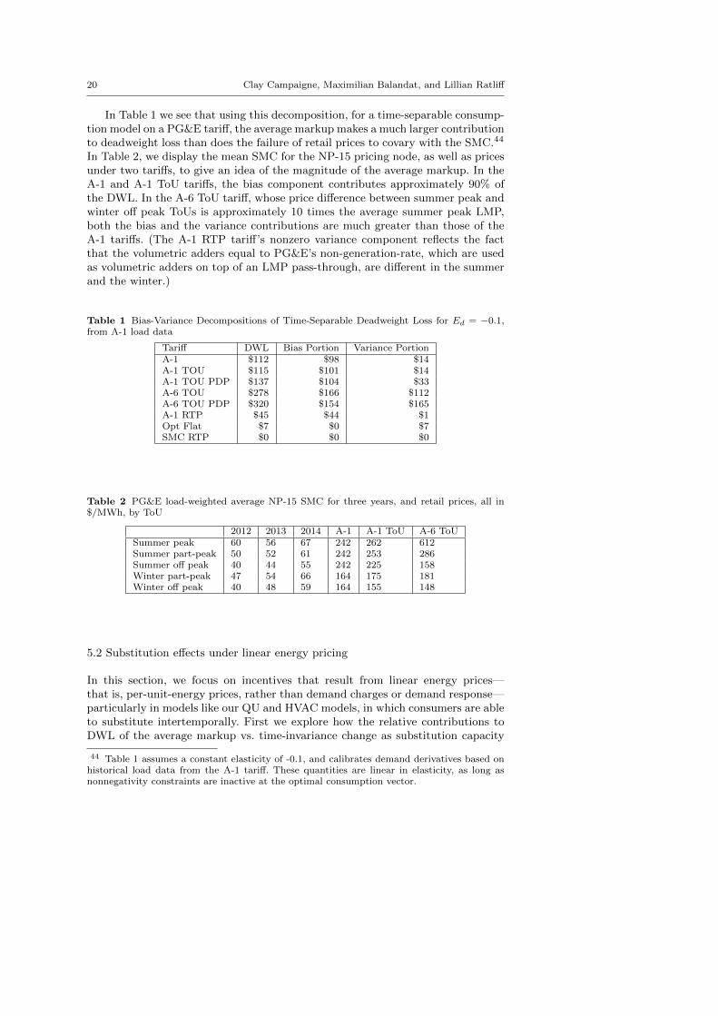
In Table 1 we see that using this decomposition, for a time-separable consump-tion model on a PG&E tariff, the average markup makes a much larger contributionto deadweight loss than does the failure of retail prices to covary with the SMC.44
In Table 2, we display the mean SMC for the NP-15 pricing node, as well as pricesunder two tariffs, to give an idea of the magnitude of the average markup. In theA-1 and A-1 ToU tariffs, the bias component contributes approximately 90% ofthe DWL. In the A-6 ToU tariff, whose price difference between summer peak andwinter off peak ToUs is approximately 10 times the average summer peak LMP,both the bias and the variance contributions are much greater than those of theA-1 tariffs. (The A-1 RTP tariff’s nonzero variance component reflects the factthat the volumetric adders equal to PG&E’s non-generation-rate, which are usedas volumetric adders on top of an LMP pass-through, are different in the summerand the winter.)
Table 1 Bias-Variance Decompositions of Time-Separable Deadweight Loss for Ed = −0.1,from A-1 load data
Tariff DWL Bias Portion Variance PortionA-1 $112 $98 $14A-1 TOU $115 $101 $14A-1 TOU PDP $137 $104 $33A-6 TOU $278 $166 $112A-6 TOU PDP $320 $154 $165A-1 RTP $45 $44 $1Opt Flat $7 $0 $7SMC RTP $0 $0 $0
Table 2 PG&E load-weighted average NP-15 SMC for three years, and retail prices, all in$/MWh, by ToU
2012 2013 2014 A-1 A-1 ToU A-6 ToUSummer peak 60 56 67 242 262 612Summer part-peak 50 52 61 242 253 286Summer off peak 40 44 55 242 225 158Winter part-peak 47 54 66 164 175 181Winter off peak 40 48 59 164 155 148
5.2 Substitution effects under linear energy pricing
In this section, we focus on incentives that result from linear energy prices—that is, per-unit-energy prices, rather than demand charges or demand response—particularly in models like our QU and HVAC models, in which consumers are ableto substitute intertemporally. First we explore how the relative contributions toDWL of the average markup vs. time-invariance change as substitution capacity
44 Table 1 assumes a constant elasticity of -0.1, and calibrates demand derivatives based onhistorical load data from the A-1 tariff. These quantities are linear in elasticity, as long asnonnegativity constraints are inactive at the optimal consumption vector.
Welfare Effects of Dynamic Electricity Pricing 21
changes, either “directly,” via cross-price elasticity, or “indirectly,” by load-shiftingusing either existing means of storage (HVAC model) or a battery (QU model).45
Then we draw a distinction between “level effects” and “load shifting effects” oftariffs on consumption patterns, which helps us explain why some tariffs have theefficiency effects that they do.
For a consumer with the ability to intertemporally substitute, the bias-variancedecomposition introduced above no longer exhausts the deadweight loss. Never-theless, we can still consider markups and a lack of real-time pricing as two prin-cipal factors impacting tariff efficiency, and compare their effects. We present twoarguments to demonstrate that, as we increase cross-price elasticity directly orindirectly, the high level of markups diminishes in importance, and the lack of realtime pricing — which is in a sense the same thing as high markup variance —becomes more important.
First we consider changing cross-price elasticity directly in a linear demandmodel. Examining the cross terms in equation (6), we see that, roughly speaking,the more highly correlated tariff errors are for pairs of periods which serve as sub-stitutes (i.e., have large positive cross-price elasticities), the more the substitutioneffect reduces deadweight loss. On the other hand, if two pricing errors have op-posite signs in substitute hours, then they induce inefficient substitution betweentheir respective hours. Using (6), we can derive a condition for a two-good lineardemand system under which, even if both pricing errors are positive, increasingthe smaller of them can reduce deadweight loss:46
∂
∂e1
(e21∂x1
∂e1+ e22
∂x2
∂e2+ e1e2
(∂x1
∂e2+∂x2
∂e1
))> 0⇔ e2
e1> −2
∂x1/∂e1∂x1
∂e2+ ∂x2
∂e1
. (7)
This inequality shows that, if the markup of good 2 is high compared to thatof good 1, and the cross-price elasticities are large compared to good 1’s own-priceelasticity, then increasing the magnitude of e1 can actually reduce deadweight loss,by diminishing exaggerated incentives to substitute good 1 for good 2 (recall that∂x1/∂e1 < 0, and generally, the cross-price elasticities are positive). The lesson isthat equalizing markups across time becomes more important as cross-elasticityincreases.47
Now we consider the effect of changing cross-price elasticity “indirectly,” byvarying the size of the Quadratic Utility consumer’s battery, between None, Medium,and Large.48 We see how this indirect modification of cross-price elasticity affects
45 In our QU model, we use the battery model as an indirect means of introducing cross-price elasticity. The QU-with-battery demand system is piecewise linear, rather than linear,and so equation (6) is only an approximation to the DWL. For the HVAC model, if therewere no heat dissipation, then as long as constraints are not binding, the consumer will shiftconsumption to the cheapest period. This means that, effectively, the cross price-elasticitywould be infinite between two periods with different price as long as consumption can beshifted without violating the constraints. In reality, heat dissipation renders it finite, althoughpotentially very high.46 The derivation relies on the linearity of the demand system, i.e., the fact that higher-order
derivatives of demand quantities with respect to price are zero.47 The argument that substitution between goods drives their optimal markups together has
a long history in the taxation literature. Hatta and Haltiwanger (1984), for example, givesufficient conditions on the “strength” of substitutes, which guarantee that “squeezing” theirtax rates toward each other would be welfare-improving.48 See Appendix B.1

22 Clay Campaigne, Maximilian Balandat, and Lillian Ratliff
the relative contributions of average markup and correlation with RTP changeby comparing the DWL under two hypothetical tariffs. The A-1 RTP tariff has aconstant markup to recover fixed costs (no markup variance), so that its DWL isentirely attributable to markups. On the other hand, the “Opt Flat” tariff doesnot track SMC variation at all, but has an average markup of zero, so that itsDWL is entirely attributable to a lack of real-time pricing.49
In Figure 1, we present the result of this analysis, for elasticity Ed = −0.1.On the x-axis, we plot the deadweight loss in each tariff that results from a time-separable model, such as those assumed by Borenstein and Holland (2005) andHogan (2014); this is calculated directly from equation (6), without intertemporalcross-terms, using tariff data and utility function parameters. On the y-axis, weplot the deadweight loss from our simulation results relative to the social surplusunder the “SMC-RTP” tariff, with the same elasticity and battery technology.50 InFigure 1, circle markers represent no substitution (no battery), diamond markersrepresent moderate substitution (Medium battery), and inverted triangle markersrepresent high substitution (Large battery). Each tariff is represented as a verticalstack of three markers, one of each shape, because the x-axis quantity does notaccount for substitution capability. The fact that the circle markers lie on they = x line shows that our consumption model is correctly calibrated.51
In the left portion of the figure, we see that without substitution, the Opt Flattariff has a much lower DWL than the A-1 RTP (see also Table 1). But as weallow and increase substitution by introducing and then increasing the size of thephysical battery model, the Opt Flat tariff induces much larger DWLs. This isbecause the Opt Flat tariff fails to encourage efficient intertemporal substitution,while the A-1 RTP tariff promotes it.
The corresponding results for several actual PG&E commercial tariffs appearin the right portion of Figure 1. These tariffs are less efficient than the hypotheticaltariffs described so far.
49 The optimal flat tariff, assuming time-separable consumption utility, weights SMCs bytheir demand derivatives: see equation (5) in Borenstein and Holland (2003). However, as we usethe same tariffs for several different consumer types, we reflect our agnosticism about demandby using an arithmetic average. This discrepancy accounts for the fact that the bias componentis not exactly zero. Another reasonable choice might be to use system load weighting, to assurethat energy costs are recovered by the LSE.50 This comparison assumes that technology is fixed. If we interpret the battery as a proxy
for other kinds of substitution preferences, then the comparison would hold those constant aswell.51 However, if we displayed the same plot for Ed ≤ −0.2, the DWL predicted by equation
(6) would overstate the actual DWL for PDP tariffs, because that equation is only valid for“interior solutions,” whereas PDP prices get so high that they drive the optimal unconstrainedconsumption quantities negative for elastic consumers.
Welfare Effects of Dynamic Electricity Pricing 23
A-6 TOU
A-6 TOU PDP
A-1 TOU PDP
A-1 TOU
A-1A-1 RTP
Opt FlatSMC RTP
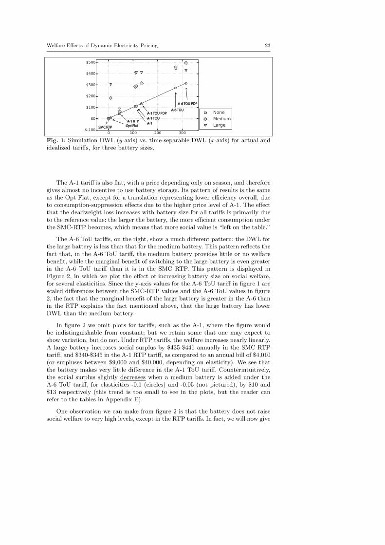
Fig. 1: Simulation DWL (y-axis) vs. time-separable DWL (x-axis) for actual andidealized tariffs, for three battery sizes.
The A-1 tariff is also flat, with a price depending only on season, and thereforegives almost no incentive to use battery storage. Its pattern of results is the sameas the Opt Flat, except for a translation representing lower efficiency overall, dueto consumption-suppression effects due to the higher price level of A-1. The effectthat the deadweight loss increases with battery size for all tariffs is primarily dueto the reference value: the larger the battery, the more efficient consumption underthe SMC-RTP becomes, which means that more social value is “left on the table.”
The A-6 ToU tariffs, on the right, show a much different pattern: the DWL forthe large battery is less than that for the medium battery. This pattern reflects thefact that, in the A-6 ToU tariff, the medium battery provides little or no welfarebenefit, while the marginal benefit of switching to the large battery is even greaterin the A-6 ToU tariff than it is in the SMC RTP. This pattern is displayed inFigure 2, in which we plot the effect of increasing battery size on social welfare,for several elasticities. Since the y-axis values for the A-6 ToU tariff in figure 1 arescaled differences between the SMC-RTP values and the A-6 ToU values in figure2, the fact that the marginal benefit of the large battery is greater in the A-6 thanin the RTP explains the fact mentioned above, that the large battery has lowerDWL than the medium battery.
In figure 2 we omit plots for tariffs, such as the A-1, where the figure wouldbe indistinguishable from constant; but we retain some that one may expect toshow variation, but do not. Under RTP tariffs, the welfare increases nearly linearly.A large battery increases social surplus by $435-$441 annually in the SMC-RTPtariff, and $340-$345 in the A-1 RTP tariff, as compared to an annual bill of $4,010(or surpluses between $9,000 and $40,000, depending on elasticity). We see thatthe battery makes very little difference in the A-1 ToU tariff. Counterintuitively,the social surplus slightly decreases when a medium battery is added under theA-6 ToU tariff, for elasticities -0.1 (circles) and -0.05 (not pictured), by $10 and$13 respectively (this trend is too small to see in the plots, but the reader canrefer to the tables in Appendix E).
One observation we can make from figure 2 is that the battery does not raisesocial welfare to very high levels, except in the RTP tariffs. In fact, we will now give

24 Clay Campaigne, Maximilian Balandat, and Lillian Ratliff
0.90
0.95
1.00
1.05SMC RTP A1 RTP A1 BLT
0.90
0.95
1.00
1.05A1TOU A1TOU BLT A1TOU PDP
N M L0.90
0.95
1.00
1.05A6TOU
N M L
A6TOU BLT
N M L
A6TOU PDP
Ed =-0.1
Ed =-0.2
Ed =-0.3
Fig. 2: Quadratic Utility: Normalized Social Surplus (disregarding capacity costs)for Battery Size = (N)one, (M)edium, and (L)arge, for 9 tariff × DR type combina-tions. Social surplus is normalized by value for SMC RTP, with the correspondingelasticity and no battery.
an argument that even the substantial social welfare gains from increasing batterysize in the A-6 ToU tariff are not due to efficient use of the battery itself.52
To make this argument, we decompose the deadweight loss into “level effects”and “load-shifting effects.” That is, we distinguish between (i) whether the con-sumption levels in each period are efficient, and (ii) whether, given those levels,the use of the battery is efficient.53 This decomposition is expressed in the equalitybetween (8) and (9) below.
Defining the “virtual social energy arbitrage revenue” (VSEAR) as the so-cial benefit from shifting energy across time without changing consumption lev-els,54 the inefficiency of suboptimal use of storage can be expressed as the efficientVSEAR, minus the VSEAR under individually optimal behavior, resulting in theequality between (9) and (10) below:
52 Neubauer and Simpson (2015) make a similar argument, that demand charges give con-sumers inefficient incentives to exploit on-site storage.53 These are features of consumption decisions given the ability for intertemporal substitu-
tion, rather than tariffs, and are distinct from the bias-variance decomposition of DWL thatis applicable for time-separable consumption models.54 i.e., VSEAR =
∑t(u2,t − u1,t)SMCt according to the notation from Section 3.2.1, and
VPEAR, defined below is∑
t(u2,t − u1,t)pRt .

Welfare Effects of Dynamic Electricity Pricing 25
DWL = Efficient Surplus−Actual Surplus (8)
= (Efficient Surplus−Actual Levels Efficiently Sourced︸ ︷︷ ︸DWL from consuming at inefficient levels: ≥0
)
+ (Actual Levels Efficiently Sourced−Actual Surplus︸ ︷︷ ︸DWL from inefficient battery use given actual consumption levels: ≥0
) (9)
= (Efficient Surplus−Actual Levels Efficiently Sourced︸ ︷︷ ︸DWL from consuming at inefficient levels: ≥0
)
+ (Actual Levels Efficiently Sourced−Actual Levels No Battery︸ ︷︷ ︸VSEAR given actual consumption but socially optimal shifting: ≥0
)
+ (Actual Levels No Battery−Actual Surplus︸ ︷︷ ︸−VSEAR under individually optimal behavior
) (10)
The first two summands in (10) are nonnegative by construction, but theircalculation requires an auxiliary optimization which we do not perform. The lastterm is, in a sense, the impact of actual (individually optimal) battery use oneconomic efficiency.
For intuition about the cause of inefficient substitution, consider a consumerthat will consume a unit of energy in hour i, and has the option of drawing thatunit from the grid either in hour i, or drawing a slightly larger quantity to providefor that consumption in hour j < i. (That is, we hold the consumption quantityconstant, as in the latter components of the decompositions above.) The con-sumer’s battery has charge, discharge, and leakage inefficiencies, ηc, ηd and Tleak
respectively. The consumer saves the following dollar quantity per unit if it choosesto draw the power in period j < i:
pRi −pRj
ηdηce(i−j)/Tleak≈ pRi − 1.11 · 1.01(i−j)pRj ≈ p
Ri − (1.11 + 0.01(i− j))pRj .
(11)
We refer to (11), summed over time indices, as the virtual private energy ar-bitrage revenue, or VPEAR.55 The middle expression of (11) plugs in our batterymodel parameters. Because (1.01)k ≈ 1 + .01 k for small k, battery storage effec-tively increases the price and cost by a fixed 11% for a charge-discharge cycle, plus1% per hour in storage, compared to the price and cost in the actual productionhour.
The social cost savings from that substitution is the same expression with thecorresponding social marginal costs in place of retail prices:
SMCi −SMCj
ηdηce(i−j)/Tleak. (12)
55 This measure only includes energy charges, and is thus not an accurate measure of expen-diture savings for tariffs with DR or demand charges. However, it is valid for peak day pricing,since we model PDP as part of the energy charge of the tariff.
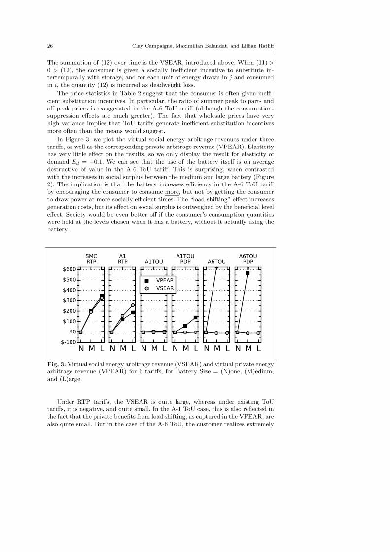
26 Clay Campaigne, Maximilian Balandat, and Lillian Ratliff
The summation of (12) over time is the VSEAR, introduced above. When (11) >0 > (12), the consumer is given a socially inefficient incentive to substitute in-tertemporally with storage, and for each unit of energy drawn in j and consumedin i, the quantity (12) is incurred as deadweight loss.
The price statistics in Table 2 suggest that the consumer is often given ineffi-cient substitution incentives. In particular, the ratio of summer peak to part- andoff peak prices is exaggerated in the A-6 ToU tariff (although the consumption-suppression effects are much greater). The fact that wholesale prices have veryhigh variance implies that ToU tariffs generate inefficient substitution incentivesmore often than the means would suggest.
In Figure 3, we plot the virtual social energy arbitrage revenues under threetariffs, as well as the corresponding private arbitrage revenue (VPEAR). Elasticityhas very little effect on the results, so we only display the result for elasticity ofdemand Ed = −0.1. We can see that the use of the battery itself is on averagedestructive of value in the A-6 ToU tariff. This is surprising, when contrastedwith the increases in social surplus between the medium and large battery (Figure2). The implication is that the battery increases efficiency in the A-6 ToU tariffby encouraging the consumer to consume more, but not by getting the consumerto draw power at more socially efficient times. The “load-shifting” effect increasesgeneration costs, but its effect on social surplus is outweighed by the beneficial leveleffect. Society would be even better off if the consumer’s consumption quantitieswere held at the levels chosen when it has a battery, without it actually using thebattery.
N M L$-100
$0
$100
$200
$300
$400
$500
$600
SMCRTP
N M L
A1RTP
N M L
A1TOU
N M L
A1TOUPDP
VPEAR
VSEAR
N M L
A6TOU
N M L
A6TOUPDP
Fig. 3: Virtual social energy arbitrage revenue (VSEAR) and virtual private energyarbitrage revenue (VPEAR) for 6 tariffs, for Battery Size = (N)one, (M)edium,and (L)arge.
Under RTP tariffs, the VSEAR is quite large, whereas under existing ToUtariffs, it is negative, and quite small. In the A-1 ToU case, this is also reflected inthe fact that the private benefits from load shifting, as captured in the VPEAR, arealso quite small. But in the case of the A-6 ToU, the customer realizes extremely

Welfare Effects of Dynamic Electricity Pricing 27
large private benefits—about $1,300 annually—from load shifting which is in itselfsocially destructive. This pattern of results helps explains the trends in socialsurplus depicted in figure 2 above.
These observations, that existing retail tariffs do not align private incentiveswith social welfare, make us skeptical of the case for public subsidization of on-sitebattery storage. Noting the often small, mixed or unpredictable effects of batterystorage in existing tariffs, we believe that any subsidies should be conditioned onthe development of retail tariffs that give consumers reliably efficient price signals.
5.3 Simulation Results: Comparison Across Tariffs
Building on the preliminary, thematically organized analysis above, in this sectionwe summarize the cross-tariff comparison of welfare measures.
5.3.1 Quadratic Utility
First we continue discussing the results for the quadratic utility model. In Figures4 and 5, we plot dollar changes in economic surpluses, under real and hypotheticaltariffs respectively, using the A-1 tariff as a benchmark. The social surplus underthe A-1 does not depend on battery size, and is $8,855 for elasticity Ed = −0.3,$12,000 for Ed = −0.2, $21,435 for Ed = −0.10, and $40,305 for Ed = −0.05. Fora more concrete benchmark, the consumer expenditure is $4,010, and the totalof SMC and capacity cost is $1,209, regardless of elasticity or battery size.56 Alldata is presented in tables 5 - 16. We plot the changes in social surplus (thickblack arrows) as the sum of three components: change in consumer surplus on top(blue arrows), change in retailer surplus ignoring capacity costs (“retail energysurplus” — red arrows), and negative change in capacity costs on the bottom(purple arrows). We represent the summation of these components into the totalchange in social surplus in the style of “tip-to-tail” vector sum diagrams.
We do not simulate the quadratic utility model under tariffs with demandcharges (the A-10 and E-19 tariffs), because we already make a very large numberof comparisons in the QU model; calibrating the QU utility parameters by assum-ing the optimality of historical load data is much more complicated under suchtariffs; and those consumer classes associated with these tariffs seem quite differentfrom those associated to the A-1 and A-6 tariffs. For the sake of completeness, wealso plot the effect of DR under “baseline-taking equilibrium.” (We explore theeffects of DR in greater detail in Section 6.)
The most salient trends are that with low elasticities, efficiency effects arequite small, because prices have smaller effects on consumption levels57; that thelarger efficiency effects are typically across tariffs, rather than between the variousdynamic variation of each tariffs, with the Opt Flat tariff being the most efficientwith no battery and real time pricing being the most efficient with a battery,
56 The expenditure and cost are constant because the consumer parameters are calibrated toreproduce a given reference consumption trace for each elasticity, and the battery plays almostno role under the A-1 tariff.57 Recall that equation (6) shows that without intertemporal substitution, deadweight loss
is linear in elasticity when nonnegativity constraints are inactive for the optimal consumptionvector.

28 Clay Campaigne, Maximilian Balandat, and Lillian Ratliff
and the A-6 ToU tariff being the least efficient, except with a large battery. Asdiscussed in Section 5.1, without intertemporal substitution, the average level ofthe tariff is the primary driver of efficiency effects, but when there is consumptionsubstitution, the real time pricing tariffs are generally much more efficient than allother tariffs. The efficiency effects of DR under “baseline-taking equilibrium” aregenerally positive but often small. We discuss the effects of DR and its distortionsin detail in Section 6.
A1 DR
A1TOU
A1TOU PDP
A1TOU DR
A6TOU
A6TOU PDP
A6TOU DR
Ed=-0.1, Batt Size=None Ed=-0.2, Batt Size=None Ed=-0.3, Batt Size=None
A1 DR
A1TOU
A1TOU PDP
A1TOU DR
A6TOU
A6TOU PDP
A6TOU DR
Ed=-0.1, Batt Size=Medium Ed=-0.2, Batt Size=Medium Ed=-0.3, Batt Size=Medium
$-1000 $-500 $0 $500
A1 DR
A1TOU
A1TOU PDP
A1TOU DR
A6TOU
A6TOU PDP
A6TOU DR
Ed=-0.1, Batt Size=Large
∆CS∆RES
∆Cap∆SS
$-1000 $-500 $0 $500
Ed=-0.2, Batt Size=Large
$-1000 $-500 $0 $500
Ed=-0.3, Batt Size=Large
Fig. 4: Quadratic Utility model, changes in surplus from A-1 tariff benchmark;realistic tariffs.
A-1 and A-1 ToU
The A-1 tariff without DR is not represented in figure 4, because it is the baselineagainst which other tariffs are compared. The “vanilla” settings of the A-1 andA-1 ToU tariffs have nearly the same results, and are within $10 of each other forevery metric, for every elasticity and battery size.
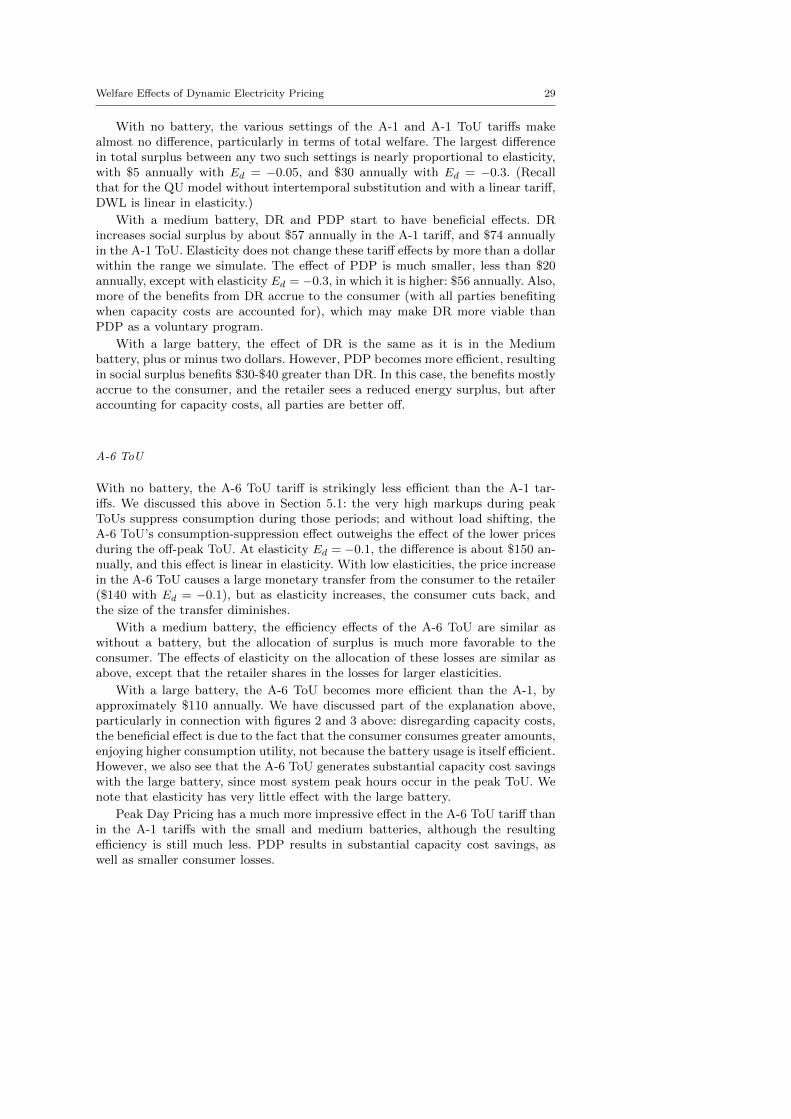
Welfare Effects of Dynamic Electricity Pricing 29
With no battery, the various settings of the A-1 and A-1 ToU tariffs makealmost no difference, particularly in terms of total welfare. The largest differencein total surplus between any two such settings is nearly proportional to elasticity,with $5 annually with Ed = −0.05, and $30 annually with Ed = −0.3. (Recallthat for the QU model without intertemporal substitution and with a linear tariff,DWL is linear in elasticity.)
With a medium battery, DR and PDP start to have beneficial effects. DRincreases social surplus by about $57 annually in the A-1 tariff, and $74 annuallyin the A-1 ToU. Elasticity does not change these tariff effects by more than a dollarwithin the range we simulate. The effect of PDP is much smaller, less than $20annually, except with elasticity Ed = −0.3, in which it is higher: $56 annually. Also,more of the benefits from DR accrue to the consumer (with all parties benefitingwhen capacity costs are accounted for), which may make DR more viable thanPDP as a voluntary program.
With a large battery, the effect of DR is the same as it is in the Mediumbattery, plus or minus two dollars. However, PDP becomes more efficient, resultingin social surplus benefits $30-$40 greater than DR. In this case, the benefits mostlyaccrue to the consumer, and the retailer sees a reduced energy surplus, but afteraccounting for capacity costs, all parties are better off.
A-6 ToU
With no battery, the A-6 ToU tariff is strikingly less efficient than the A-1 tar-iffs. We discussed this above in Section 5.1: the very high markups during peakToUs suppress consumption during those periods; and without load shifting, theA-6 ToU’s consumption-suppression effect outweighs the effect of the lower pricesduring the off-peak ToU. At elasticity Ed = −0.1, the difference is about $150 an-nually, and this effect is linear in elasticity. With low elasticities, the price increasein the A-6 ToU causes a large monetary transfer from the consumer to the retailer($140 with Ed = −0.1), but as elasticity increases, the consumer cuts back, andthe size of the transfer diminishes.
With a medium battery, the efficiency effects of the A-6 ToU are similar aswithout a battery, but the allocation of surplus is much more favorable to theconsumer. The effects of elasticity on the allocation of these losses are similar asabove, except that the retailer shares in the losses for larger elasticities.
With a large battery, the A-6 ToU becomes more efficient than the A-1, byapproximately $110 annually. We have discussed part of the explanation above,particularly in connection with figures 2 and 3 above: disregarding capacity costs,the beneficial effect is due to the fact that the consumer consumes greater amounts,enjoying higher consumption utility, not because the battery usage is itself efficient.However, we also see that the A-6 ToU generates substantial capacity cost savingswith the large battery, since most system peak hours occur in the peak ToU. Wenote that elasticity has very little effect with the large battery.
Peak Day Pricing has a much more impressive effect in the A-6 ToU tariff thanin the A-1 tariffs with the small and medium batteries, although the resultingefficiency is still much less. PDP results in substantial capacity cost savings, aswell as smaller consumer losses.
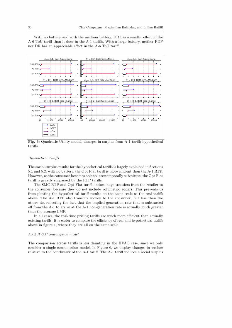
30 Clay Campaigne, Maximilian Balandat, and Lillian Ratliff
With no battery and with the medium battery, DR has a smaller effect in theA-6 ToU tariff than it does in the A-1 tariffs. With a large battery, neither PDPnor DR has an appreciable effect in the A-6 ToU tariff.
SMC-RTP
A1 RTP
Opt Flat
Ed=-0.1, Batt Size=None Ed=-0.2, Batt Size=None Ed=-0.3, Batt Size=None
SMC-RTP
A1 RTP
Opt Flat
Ed=-0.1, Batt Size=Medium Ed=-0.2, Batt Size=Medium Ed=-0.3, Batt Size=Medium
$0 $1000 $2000 $3000
SMC-RTP
A1 RTP
Opt Flat
Ed=-0.1, Batt Size=Large
∆CS∆RES
∆Cap∆SS
$0 $1000 $2000 $3000
Ed=-0.2, Batt Size=Large
$0 $1000 $2000 $3000
Ed=-0.3, Batt Size=Large
Fig. 5: Quadratic Utility model, changes in surplus from A-1 tariff; hypotheticaltariffs.
Hypothetical Tariffs
The social surplus results for the hypothetical tariffs is largely explained in Sections5.1 and 5.2: with no battery, the Opt Flat tariff is more efficient than the A-1 RTP.However, as the consumer becomes able to intertemporally substitute, the Opt Flattariff is greatly surpassed by the RTP tariffs.
The SMC RTP and Opt Flat tariffs induce huge transfers from the retailer tothe consumer, because they do not include volumetric adders. This prevents usfrom plotting the hypothetical tariff results on the same scale as the real tariffsabove. The A-1 RTP also transfers money to the consumer, but less than theothers do, reflecting the fact that the implied generation rate that is subtractedoff from the A-1 to arrive at the A-1 non-generation rate is actually much greaterthan the average LMP.
In all cases, the real-time pricing tariffs are much more efficient than actuallyexisting tariffs. It is easier to compare the efficiency of real and hypothetical tariffsabove in figure 1, where they are all on the same scale.
5.3.2 HVAC consumption model
The comparison across tariffs is less daunting in the HVAC case, since we onlyconsider a single consumption model. In Figure 6, we display changes in welfarerelative to the benchmark of the A-1 tariff. The A-1 tariff induces a social surplus
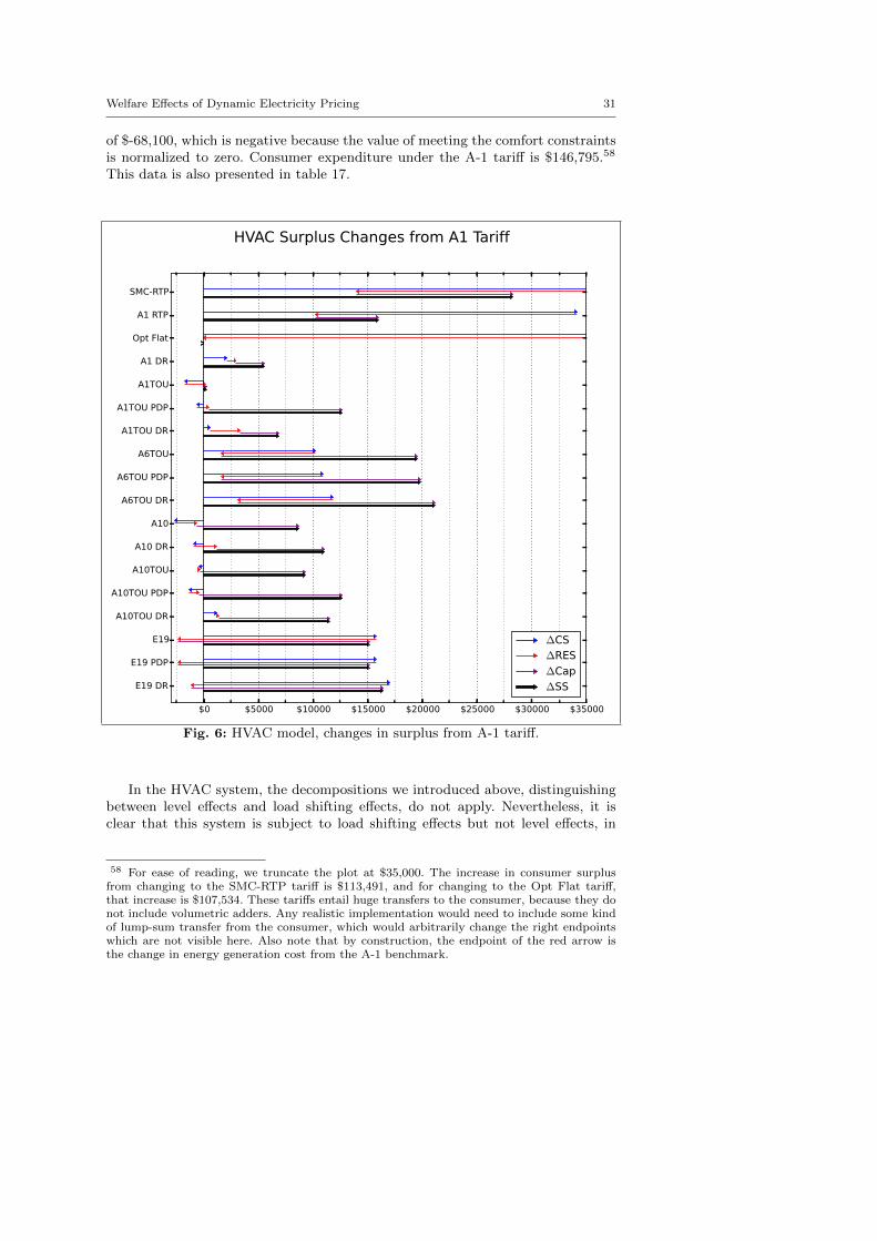
Welfare Effects of Dynamic Electricity Pricing 31
of $-68,100, which is negative because the value of meeting the comfort constraintsis normalized to zero. Consumer expenditure under the A-1 tariff is $146,795.58
This data is also presented in table 17.
$0 $5000 $10000 $15000 $20000 $25000 $30000 $35000
SMC-RTP
A1 RTP
Opt Flat
A1 DR
A1TOU
A1TOU PDP
A1TOU DR
A6TOU
A6TOU PDP
A6TOU DR
A10
A10 DR
A10TOU
A10TOU PDP
A10TOU DR
E19
E19 PDP
E19 DR
∆CS∆RES
∆Cap∆SS
HVAC Surplus Changes from A1 Tariff
Fig. 6: HVAC model, changes in surplus from A-1 tariff.
In the HVAC system, the decompositions we introduced above, distinguishingbetween level effects and load shifting effects, do not apply. Nevertheless, it isclear that this system is subject to load shifting effects but not level effects, in
58 For ease of reading, we truncate the plot at $35,000. The increase in consumer surplusfrom changing to the SMC-RTP tariff is $113,491, and for changing to the Opt Flat tariff,that increase is $107,534. These tariffs entail huge transfers to the consumer, because they donot include volumetric adders. Any realistic implementation would need to include some kindof lump-sum transfer from the consumer, which would arbitrarily change the right endpointswhich are not visible here. Also note that by construction, the endpoint of the red arrow isthe change in energy generation cost from the A-1 benchmark.

32 Clay Campaigne, Maximilian Balandat, and Lillian Ratliff
the sense that multiplying all tariff prices by a positive scalar has no effect on theconsumer’s optimal solution.59
The HVAC system results are much different from those for the quadraticutility consumer, presumably largely because of the absence of level effects.
The A-1 ToU tariff is very similar to the flat A-1, but with Peak Day Pric-ing, the A-1 ToU achieves large cost savings, of about $12,500. Every other tariffinduces a substantial improvement over the A-1 tariff, mostly because of large ca-pacity savings. This is especially the case for the A-6 and E-19 tariffs, which havevery aggressive ToU pricing. Demand Response (without baseline manipulation)is always beneficial, although the effects are largest in the A-1 and A-1 ToU tariffs.In all tariffs, PDP has positive effects — by far the most beneficial in the A-1 ToUtariff, where it saves approximately $12,500 in capacity costs.
SMC-RTP is, reassuringly, the most efficient tariff. But it is striking, and sur-prising, that the A-6 ToU tariffs are more efficient than the hypothetical A-1 RTP,and the E-19 tariffs are only slightly less efficient than the A-1 RTP. The benefitsfrom these aggressive ToU tariffs are primarily due to reductions in capacity costs,which more than compensate for less beneficial energy cost effects (as compared toA-1 RTP). This can be seen by noting that the endpoint of the red arrow representsthe change in social energy costs, and the length of the purple arrow representsthe reduction in capacity costs. The A-10 tariff has similar energy costs as the A-1tariff, but, presumably due to demand charges, it has lower capacity costs. TheE-19 tariff has consistently higher generation costs than the A-1 benchmark, butthe capacity cost savings more than compensate, so that it is also more efficientthan the A-1.
The fact that the hypothetical A-1 RTP tariff does not compare as favorablyagainst realistic tariffs as it does in the quadratic utility model, due to its smallerreductions in capacity costs than those achieved by the realistic tariffs, probablyindicates that RTP tariffs should include contribution to capacity costs, as oursimulated RTP tariffs do not. It appears that LMPs alone do not provide a suf-ficient incentive to reduce system capacity costs, particularly when their effect isdiluted by flat volumetric adders. However, we should note that our methodologyfor computing capacity costs is subject to noise, being derived from such small“samples” of hours, and it’s based on a public available dataset which we do notregard as a particularly reliable measure of actual capacity costs.60
The most dramatic pattern in private expenditures in the comparison of realtariffs is that the A-6 ToU and E-19 ToU tariffs are the cheapest for the consumer.This is because our HVAC system is very capable of intertemporal substitution,perhaps particularly in the weather regime we consider, so that the tariffs with thelowest off-peak price are the cheapest. This substitution entails a loss of retailer
59 This is because the consumer’s optimization problem is to minimize expenditure, subjectto comfort constraints. This problem can be reformulated so that the objective is linear in thevector of retail prices, with no prices showing up in the constraints. Then scaling the vector ofprices scales the objective function (by linearity) without affecting the constraints, so that theoptimal solution is unaffected. If a tariff includes complicated elements like demand responseor demand charges, prices show up in auxiliary constraints. But these constraints can beeliminated by substitution into the objective, at the cost of no longer having a standard-formLP or MIP, which only matters for computational reasons.60 One way to reduce the variance of capacity cost estimates would be to average effects
across heterogenous consumers. Another would be to adopt something like the “probabilistic”capacity charge allocation from Boomhower and Davis (2016).

Welfare Effects of Dynamic Electricity Pricing 33
energy surplus, because the retail price differences are greater than the averagewholesale price differences.
The hypothetical tariffs all induce large transfers from the retailer to the con-sumer, because realistic tariffs include such high markups over LMPs.

34 Clay Campaigne, Maximilian Balandat, and Lillian Ratliff
6 The effects of demand response and DR distortions
6.1 Theoretical Overview
In this section, we examine the welfare effects of Demand Response, with a focus ontwo economic distortions commented on in the literature: “baseline manipulation”and “double payment” (Chao and DePillis, 2013; Hogan, 2010; Borlick et al., 2012).
Baseline manipulation
A fully rational consumer who understands the baselining method may have anincentive to artificially inflate her consumption during certain periods in order toincrease the rewards from DR “reductions” during periods of high reward pDRt .In our model the baseline values are determined endogenously as part of the op-timization problem, so these incentives are captured correctly and we can indeedobserve this behavior in our simulations (see Appendix C.3). To evaluate the effectsof baseline manipulation compared to the behavior of a non-strategic customer,we consider a no-manipulation benchmark that we refer to as “baseline-takingequilibrium”:
Definition 1 (Baseline-Taking Equilibrium) Let β : q 7→ qBL denote the func-tion mapping a consumption sequence q = (q1, . . . , qT ) to a sequence of baselinevalues qBL = (qBL1 , . . . , qBLT ), and let C denote the set of constraints on state andcontrol variables of the consumer. Then (x∗,u∗,q∗) is a baseline-taking equilibriumif q∗ = β(q∗) and (x∗,u∗) ∈ arg maxx,u∈C V(x,u; q∗).
In words, a baseline-taking consumer regards the DR baseline values as exoge-nously given data, rather than decision variables as in the “fully rational” model.In equilibrium, the consumer’s optimal response to these baseline values results, ascomputed by the given baselining methodology (in our case, CAISO “10 in 10”),in the given DR baseline. That is, the vector of baseline quantities is a fixed pointof the operator β(·) in Definition 1. Algorithm 1 in Appendix A.2 describes thefixed-point iteration we use to compute a baseline-taking equilibrium.
The contrast between such a baseline-taking equilibrium and the strategic, or“baseline-manipulation” optimum is analogous to the contrast between a price-taking equilibrium on the one hand, and monopoly or Cournot oligopoly pricingoutcomes on the other.61
To illustrate baseline manipulation resulting from the distorted incentives, weshow some simulation results that highlight the effect of DR with and withoutbaseline manipulation. These plots show how a fully rational (i.e. strategic) DRparticipant would behave with advanced knowledge of DR event days, and theyalso demonstrate that optimal behavior in baseline-taking equilibrium matches anintuitive understanding of how a rational DR participant that ignores the incentiveto inflate the baseline would behave.
61 To solve for a price-taking equilibrium, the economist characterizes producers’ optimalquantity response as a function of an exogenously determined price over which the producerhas no strategic control. Then the economist uses a market-clearing condition relating pricesand total production quantities to determine the equilibrium price that supports these quantitydecision. By comparing prices and quantities in both economic environments, one can, arguably,capture the effects of strategic “manipulation” of baselines, and prices, respectively.

Welfare Effects of Dynamic Electricity Pricing 35
Baseline manipulation in the QU model
A sample solution from our simulation of the Quadratic Utility model under theOptFlat tariff is shown in Figure 2.7 for the strategic agent (CAISO), the baseline-taking agent (BLT), and the Nominal agent, who is not exposed to any DR in-centives. We highlight the DR event as well as the BL-relevant periods, i.e. theperiods that are considered for determining the baseline value for the DR period.
0
1
2
3
4
5
control input [kW]
CAISO charge
BLT charge
CAISO discharge
BLT discharge
DR event
BL-relevant
0
2
4
6
8
energy consumption [kW
h]
CAISO
BLT
Nominal
DR event
BL-relevant
12:00 00:0019-Nov2012
00:0020-Nov
00:0021-Nov
12:00 12:00 12:000
1
2
3
4
5
battery charge [kW
h] CAISO
BLT
Nominal
DR event
BL-relevant
Fig. 7: Baseline manipulation behavior in the QU model, OptFlat, medium bat-tery, Ed = −0.3
The top panel of Figure 7 shows the charging (u1) and discharging (u2) ratesof the battery.62 We see that immediately before and during the DR event, boththe strategic agent and the BLT agent act the same: before the event they chargethe battery, and then they consume from the battery during the event. The middlepanel shows the total energy drawn from the grid (u1 +u3). From this we see thatduring the DR event, both the strategic and BLT agent in fact consume exclusivelyfrom their battery and draw no power from the grid (the Nominal agent ignoresthe event). But at 24 and 48 hours before the event, the BLT agent acts the sameas the Nominal agent, while the strategic agent charges its battery as rapidly as
62 We do not include the respective inputs of the nominal agent, who under the Opt Flattariff does not use the battery and exclusively consumes energy directly from the grid.
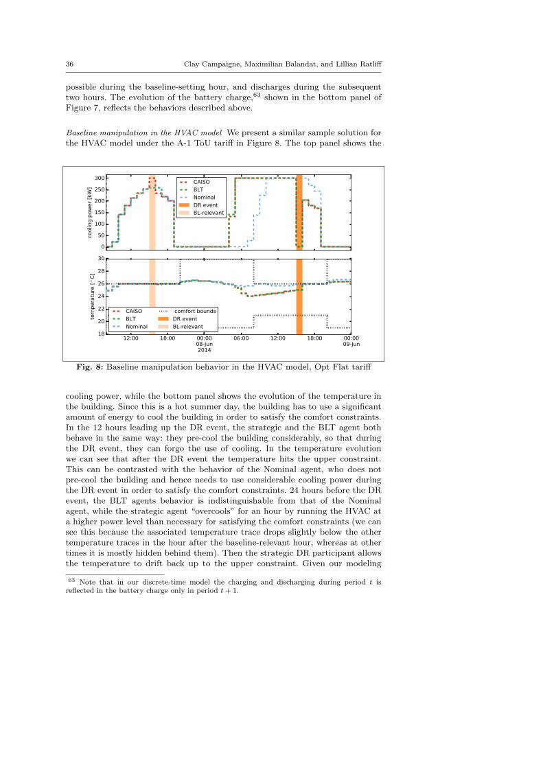
36 Clay Campaigne, Maximilian Balandat, and Lillian Ratliff
possible during the baseline-setting hour, and discharges during the subsequenttwo hours. The evolution of the battery charge,63 shown in the bottom panel ofFigure 7, reflects the behaviors described above.
Baseline manipulation in the HVAC model We present a similar sample solution forthe HVAC model under the A-1 ToU tariff in Figure 8. The top panel shows the
0
50
100
150
200
250
300
cooling power [kW]
CAISO
BLT
Nominal
DR event
BL-relevant
00:0008-Jun2014
00:0009-Jun
12:00 18:00 06:00 12:00 18:0018
20
22
24
26
28
30
tem
pera
ture
[◦ C
]
CAISO
BLT
Nominal
comfort bounds
DR event
BL-relevant
Fig. 8: Baseline manipulation behavior in the HVAC model, Opt Flat tariff
cooling power, while the bottom panel shows the evolution of the temperature inthe building. Since this is a hot summer day, the building has to use a significantamount of energy to cool the building in order to satisfy the comfort constraints.In the 12 hours leading up the DR event, the strategic and the BLT agent bothbehave in the same way: they pre-cool the building considerably, so that duringthe DR event, they can forgo the use of cooling. In the temperature evolutionwe can see that after the DR event the temperature hits the upper constraint.This can be contrasted with the behavior of the Nominal agent, who does notpre-cool the building and hence needs to use considerable cooling power duringthe DR event in order to satisfy the comfort constraints. 24 hours before the DRevent, the BLT agents behavior is indistinguishable from that of the Nominalagent, while the strategic agent “overcools” for an hour by running the HVAC ata higher power level than necessary for satisfying the comfort constraints (we cansee this because the associated temperature trace drops slightly below the othertemperature traces in the hour after the baseline-relevant hour, whereas at othertimes it is mostly hidden behind them). Then the strategic DR participant allowsthe temperature to drift back up to the upper constraint. Given our modeling
63 Note that in our discrete-time model the charging and discharging during period t isreflected in the battery charge only in period t+ 1.

Welfare Effects of Dynamic Electricity Pricing 37
assumption that the buildings occupants are indifferent to temperature as long asit satisfies the comfort constraints, this overcooling behavior is wasteful, becausethe energy needed to maintain a certain temperature level is greater the furtherit is from the temperature the building would be without actuation.64
In both the QU and the HVAC cases, the baseline-taking and baseline-manipulatingbehavior are indistinguishable in hours leading up to the DR event, when “legiti-mate” preparation for DR event occurs. Obviously, manipulation behavior occurs24 hours prior, 48 hours, and so on. This has an important and intuitive im-plication of what we might expect when there is price uncertainty that resolvesas the hour approaches: if the day-ahead forecast is good, then as uncertainty isintroduced into further-ahead forecasts, baseline-manipulation behavior should di-minish, and the strategic agent should become more similar to the baseline-takingagent. This is because baseline-manipulation is costly, because by definition theagent is deviating from behavior that would be optimal if not for the effect on thebaseline.
Double payment
The other economic distortion we consider is “double payment.” Under the com-pensation scheme mandated by FERC Order 745, providers of demand responseare to be paid for reductions from their historical baseline at the LMP. But byreducing consumption, the DR participant also avoids paying the retail price, pRt .The retail price can be decomposed into a component that reflects the averagecost of energy procurement, plus a markup intended to recoup the retailer’s ad-ditional costs, particularly their fixed costs. We can write this decomposition aspRt = E[pWt ]+T&Dt, where the first term denotes the average wholesale price, andthe second denotes fixed costs such as Transmission and Distribution.
The result is that, in a DR hour, the the avoided expenditure, or effective “netprice” per MWh reduced, is pRt + pWt = E[pWt ] + T&Dt + pWt , which exceeds theefficient price by E[pWt ] + T&Dt. But in an average hour, the retail price exceedsthe efficient price by only T&Dt.
65
Many economists have concluded on the basis of this and other argumentsthat this effective price during DR events is too high, incentivizing inefficientlylow consumption levels (Borlick et al., 2012; Chao and DePillis, 2013); and that ifbaseline-dependent DR is to exist, a quantity, usually referred to as “G,” shouldbe subtracted from the DR payment, to correct the effective price.
However, there is a lack of clarity in the literature about what exactly this “G”should be. Some authors take it to be the retail rate (Chao and DePillis (2013);Borlick et al. (2012); Borlick (2010); Shanker (2010)), so that the effective price
64 If the only exogenous determinants of building temperature were outside temperature, thiswould be the simple result of Newtons law of cooling, which states that the rate at which abody dissipates heat into its surroundings is proportional to the difference between the bodystemperature and that of its surroundings. In a model with higher order terms relating powerdraw and HVAC cooling output, overcooling might be wasteful because it would encourage thebuilding to run the HVAC at an inefficiently high level; but in our linear model, this is not anissue.65 This disregards externality costs. To account for externality costs, the reader can subtract
them from T&Dt in what follows. This is straightforward in our setting, because externalitycosts are essentially time-invariant in California, as natural gas is the marginal fuel in themajority of hours (see Appendix C.2 and Callaway et al. (2015)).

38 Clay Campaigne, Maximilian Balandat, and Lillian Ratliff
would be pWt in DR hours. This is the efficient price for a single hour consideredalone. But Hogan (2010) (also approvingly cited by Chao and DePillis (2013))argues that “G” refers to “the imputed generation portion of retail rates.” If theimputed generation component is E[pWt ], then the LMP - G payment would bepWt − E[pWt ], and the effective net price would T&Dt + pWt .
When we simulate the elimination of the double payment distortion by makingLMP-minus-G payments in our study, we adopt a variant of this latter approachsubtracting an imputed generation component of the retail price from the LMPpayment. This seems sensible because it equalizes average markups across DR andnon-DR hours (see Section 5.2), and DR does not necessarily abate fixed costs(although that point is arguable).
To derive the imputed generation component of a retail tariff, we subtractthe “non-generation rate” for that tariff from the tariff itself. The non-generationrate is a surcharge paid to PG&E by customers of Community Choice Aggregationcustomers, to cover PG&E’s infrastructure costs (see Table 3). In our hypotheticalOpt Flat tariff, we take the imputed generation component to be the average LMPitself, since the Opt Flat tariff represents the average generation rate.
Table 3 Load-weighted average A-1 ToU prices, Non-gen component, and NP-15 SMC, all in$/MWh. Data from Pacific Gas and Electric Company (a)
Tariff Non-gen Imputed gen Average SMCSummer peak 262 128 134 61Summer part-peak 253 128 125 55Summer off peak 225 128 97 46Winter part-peak 175 97 77 55Winter off peak 155 97 58 48
While we consider this to be a reasonable and realistic way of decomposingPG&E’s tariffs into generation and non-generation components, the resulting de-composition results in generation components that are much higher than the av-erage LMP.66 The resulting value of “G” is a sort of compromise, intermediatebetween the retail rate itself endorsed by Chao and DePillis (2013) on the highside, and the average wholesale price, which is perhaps the lowest value suggestedby Hogan (2010), on the low side. It seems the fact that PG&E’s imputed gen-eration component is so much higher than the average LMP is accounted for byCPUC mandates to procure various expensive renewable resources, such as wind,solar, and biogas energy, using out-of-market feed-in tariffs.67
6.2 Simulation Results: DR distortions
In the following two sections, we present our findings on the effects of DR withand without the two economic distortions just introduced, for both the quadraticutility model and the HVAC model.
66 A reasonable alternative would be some kind of load-weighted average LMP (since PG&Epublishes representative consumption data for each customer class (Pacific Gas and ElectricCompany, 2016a), a separate load-weighting measure could be used for each tariff).67 See Senate Bill 1122 (California State Senate, 2012), as well as Pacific Gas and Electric
Company (2016d).

Welfare Effects of Dynamic Electricity Pricing 39
In Figures 9 and 10, we plot, for both consumer models, the welfare effectsof the four DR settings: standard DR with both the manipulation and doublepayment distortions (“DR”); DR without double payment (“LMP-G”); DR in abaseline-taking equilibrium (“BLT”); and DR without double payment and in abaseline-taking equilibrium (“BLT & LMP-G”). The welfare effects are representedin terms of their changes (in $) from the no-DR benchmark, as in the previousfigures.
We explore the welfare impacts of these different demand response environ-ments under two tariffs: A-1 ToU and Opt Flat. We choose the A-1 ToU tariffas representative of extant tariffs, as flat tariffs such as the A-1 are being phasedout for commercial and industrial tariffs, and are not available to customers withsmart meters (Pacific Gas and Electric Company, b). We choose the Opt Flat tariffbecause it is common in the DR and dynamic pricing literature to treat DR assuperimposed on a second-best tariff, i.e. in which the retail price is the averagesocial marginal cost (Chao and DePillis, 2013, Appendix A).
Note that, in our model, DR can never have a detrimental effect on the con-sumer surplus, because participation is voluntary and we assume that the consumerhas perfect foresight.
6.2.1 DR and Distortions Simulation Results: Quadratic utility model
In general, the changes in surplus due to DR for the quadratic utility consumptionmodel are on the order of several hundred dollars at most. This is very small as afraction of total social surplus since calibration of inelastic utility functions resultsin very large social surpluses (ranging from $8,855 for elasticity Ed = −0.3 to$21,435 at elasticity Ed = −0.1). However, in absolute terms, or as a fraction ofthe annual electricity bill (calibrated to be equal to $4,013 annually in the A-1case), the changes are more substantial.
In Figure 9, we plot the results for a demand elasticity of Ed = −0.1. The plotsfor the range from -0.05 to -0.2 are very similar for both tariffs, so we only includeone.68 Since the effects of DR are almost negligible without battery storage, thislack of dependence on demand elasticity suggests that the economically significanteffects of DR are a result of battery storage arbitrage, and are mostly financialfrom the consumer’s perspective, without much effect on end-use consumptionquantities.
DR has an appreciable effect on the surpluses whenever there is battery storage.In these cases, manipulation of the DR baseline has a comparatively large anddetrimental effect on social surplus. That is, “BLT” always has a higher surplusthan “DR,” and “BLT & LMP-G” always has a higher social surplus than “LMP-G.” Whenever DR with baseline manipulation has a non-negligible effect, theconsumer benefits are much greater than for the corresponding BLT case, butthe aggregate social benefits are smaller, which implies a financial transfer fromthe retailer (really, the rest of society) to the consumer, which is sometimes quitelarge.69 In baseline-taking equilibria, the retailer surplus increases under the A-1
68 In the tables in Appendix E we also present results for Ed = −0.3, but this case is moreextreme, and perhaps not very realistic.69 Ignoring capacity costs, this transfer is the length of overlapping blue and red arrows.
Accounting for capacity costs, one would replace the red arrows with the sum of the red and

40 Clay Campaigne, Maximilian Balandat, and Lillian Ratliff
DR
LMP-G
BLT
BLT & LMP-G
A-1 TOU, Battery Size = None Opt Flat, Battery Size = None
∆CS∆RES
∆Cap∆SS
DR
LMP-G
BLT
BLT & LMP-G
A-1 TOU, Battery Size = Medium Opt Flat, Battery Size = Medium
$-200 $-100 $0 $100 $200 $300 $400 $500
DR
LMP-G
BLT
BLT & LMP-G
A-1 TOU, Battery Size = Large
$-200 $-100 $0 $100 $200 $300 $400 $500
Opt Flat, Battery Size = Large
Fig. 9: Quadratic Utility Social Surplus Changes, DR and Distortions, Ed = −0.1
ToU tariff, and is unaffected under the Opt Flat tariff. The retailer benefits areentirely due to reduction in capacity costs (purple arrows).
Without a battery, DR is beneficial to society, but the scale is negligible: atmost $15 annually (a little over $1 a month) under the very high elasticity Ed =−0.2, and at most $3 annually under the more plausible elasticity of Ed = −0.05.The largest effect of DR without a battery (and the only one greater than $15annually) is a reduction in generation cost of $36 annually, when Ed = −0.3.
With a medium battery, all DR variants increase social surplus, with an in-crease between $50 and $75 in the A-1 ToU tariff, and between $19 and $60 in theOpt Flat tariff. The lower ends of these ranges come from the baseline manipu-lation cases, and the upper ones are from baseline-taking. Eliminating the doublepayment distortion (“LMP-G” vs. “DR”, and “BLT & LMP-G” vs. “BLT”) has asmall positive effect (sometimes none) on total surplus, and has a more substantialeffect of redistributing part of the change in social surplus from the consumer tothe retailer (reducing the size of the transfer from the retailer to the consumer inthe baseline manipulation case, and magnifying the retailer’s revenue increase un-der baseline-taking). In the basic DR setting (with both manipulation and doublepayment), DR increases the social surplus by $20 annually, but involves a transferfrom the retailer to the consumer of $60 to $65 in the A-1 ToU and $140 in theOpt Flat, annually. In the real world, much of such a transfer would likely involvecross-subsidization from consumers who do not participate in DR. But withoutbaseline manipulation, both the retailer and the consumer see improvements fromDR, which is what one would hope for from a DR program.
With a large battery, the effects of DR are quite large and mixed. Strikingly,increasing the battery size from Medium to Large has a negligible effect on totalsurplus in baseline-taking equilibria, and has a large negative effect when manipu-lation is possible (comparing results for the Large vs Medium battery). With both
purple arrows. Note that for any tariff, the transfer between the consumer and the retailercould be changed to any desired values by changing the fixed charges, i.e., the meter charges.
Welfare Effects of Dynamic Electricity Pricing 41
manipulation and double payment, DR has a small negative effect on social sur-plus in the A-1 ToU tariff ($10 annually), and a larger negative effect in the OptFlat tariff ($190 annually). These totals include large transfers from the retailer tothe consumer: about $220 and $380 respectively. Without manipulation, societygains $60 to $70 annually from DR, and the retailers revenues either increase orare unaffected, as compared to no DR.
Comparing the A-1 ToU tariff with the Opt Flat tariff, we see that the deleteri-ous effects of baseline manipulation are much greater in the Opt Flat. Intuitively,this would seem to be because baseline manipulation requires “excessive” con-sumption in anticipation of upcoming DR events. That excessive consumption iseasier to engage in, in a tariff that has much lower markups, such as the Opt Flat.
These results compare DR tariffs against the A-1 ToU benchmark, whichchanges slightly with battery size. So we also summarize the effects of increasingthe battery size on social surplus in DR tariffs: With demand response, increas-ing battery size can increase social welfare by between $23 and $36 annually inthe A-1 tariff, and $44-$48 in the A-1 ToU (the high end of the ranges are fromlower elasticities). The private gains are smaller. With baseline manipulation, amedium battery realizes a value to society of $14-$26, but with a large battery, thesurplus decreases by $21-$26 annually. In conjunction with our discussion above,this suggests that RTP tariffs may make battery investments worthwhile, but DRprograms probably do not justify them, and may even make the operation of abattery economically destructive.
To sum up, in the quadratic utility model, the effects of DR on total surplusare highly dependent on the base tariff (A-1 ToU vs. Opt Flat), the size of thebattery, and the type of economic distortions allowed for, but are not significantlydependent on elasticity. Baseline manipulation is always worse for society thanbaseline taking, and can in fact make the net social effects of DR deleterious. DRwith baseline manipulation results in large transfers toward the consumer wheneverthere is any effect on efficiency. Double payment has smaller efficiency effects,mostly redistributing changes in surplus from the retailer to the consumer.70 Alarge battery as compared to a medium battery is good for the consumer, butneutral for society in baseline-taking equilibrium, and bad for society when baselinemanipulation is possible.
As a side-note, the non-monotonicity of the effect of the battery size on socialsurplus reflects the complexity of tariff incentive effects when consumers can in-tertemporally substitute, an issue we explored earlier in Section 5.2, particularlyFigures 2 and 3, with respect to the A-6 ToU tariff.
6.2.2 DR Distortions Simulation Results: HVAC model
Figure 10 shows the changes in surpluses for the HVAC model, from the no-DRbenchmarks for the A-1 and Opt Flat tariffs respectively. For the A-1 tariff, thebenchmark social surplus (negative generation cost minus capacity cost with noDR) is -$68,100, and the individual expenditure is $146,795. For the Opt Flat tariff,
70 The notable exception to this is in the A-1 ToU tariff, with the large battery and base-line manipulation, where eliminating double payment creates a $25 annual gain for society,transforming effects that were slightly or negligibly deleterious into effects that are noticeablypositive.

42 Clay Campaigne, Maximilian Balandat, and Lillian Ratliff
the social surplus benchmark is nearly same as that of the A-1 tariff (-$68,097),and the individual expenditure is $39,261.71
-1000 0 1000 2000 3000 4000 5000 6000 7000 8000
DR
LMP-G
BLT
BLT & LMP-G
HVAC: A-1 TOU
-5000 0 5000 10000
DR
LMP-G
BLT
BLT & LMP-G
HVAC: Opt Flat
∆CS∆RES
∆Cap∆SS
Fig. 10: HVAC DR distortions: Social Surplus Changes from no-DR baseline.(Benchmark social cost of generation and capacity: $68,100.)
Under the A-1 ToU tariff, the effect of demand response is always beneficialfor society in aggregate. It is also beneficial in every component of social surplus,except in the case with both DR distortions, in which case the retailer is negativelyimpacted in terms of energy costs, but in turn sees a larger benefit in terms ofcapacity costs. The pattern of results stemming from distortions is hard to explain:eliminating baseline manipulation is good for society in the presence of the doublepayment distortion, but it is deleterious for society under LMP-G compensation.Similarly, eliminating double payment is beneficial under baseline manipulation,but it is harmful in baseline-taking equilibria. And the “undistorted” outcome withbaseline-taking and LMP-G, is the worst of all four combinations of distortions.
In the Opt Flat tariff, the effects are much more concordant with economicintuition. This might be expected, since the Opt Flat tariff is the standard settingunder which DR is studied, and we do not have to worry about the interaction ofthe DR incentives with high markups and potentially distorted time-of-use priceratios. Demand response is deleterious for society with baseline manipulation,but beneficial in baseline-taking equilibrium. What is striking is the extremelyhigh transfer from the retailer to the consumer under baseline manipulation (notethough that reduced capacity costs still have a significant positive effect on retailersurplus). Eliminating the double payment distortion is beneficial under baselinemanipulation. In baseline-taking equilibrium, eliminating double payment has a
71 Since the A-1 tariff is also flat, the only difference in incentives between the two tariffs isthe incentive to substitute between summer and winter seasons in the A-1 tariff, which is onlypossible for a few hours annually. The Opt Flat individual expenditure is lower than the socialcost of generation because the Opt Flat tariff does not reflect capacity costs.

Welfare Effects of Dynamic Electricity Pricing 43
small effect, which is almost entirely a redistribution of revenue from the consumerto the retailer. This suggests that double payment does not have a large effect onconsumption behavior in baseline-taking equilibrium.
And again, baseline manipulation is a much smaller problem in the A-1 ToUtariff than it is in the Opt Flat tariff, presumably because baseline inflation is moreexpensive in the former tariff, which has much higher markups. Finally, we recallour comment from discussing the examples of baseline manipulation depicted infigures 7 and 8: it seems likely that under uncertainty about hours far in thefuture, the effects of baseline manipulation, insofar as they differ from baselinetaking, would be smaller than what we see in our simulation results.
7 Discussion
Throughout this paper, we have observed that, not all too surprisingly, the effi-ciency effects of different tariffs depend strongly on the underlying consumptionmodel. Moreover, tariffs and intertemporal substitution technology interact to pro-duce complicated patterns of outcomes, which are often hard to explain, let aloneforesee:
– Without intertemporal substitution capacity, high markups are much moreimportant drivers of welfare losses than a lack of real-time pricing, but withintertemporal substitution capacity, high markups are less important;
– With a large battery, DR with baseline manipulation is welfare-improving withhigh markups (A-1 ToU tariff), but welfare-reducing with low markups (OptFlat tariff);
– In the A-6 ToU tariff (with large price differences between ToUs), a mediumbattery provides very little social benefit, but a large battery provides a largesocial benefit. Consequently, the A-6 tariff reduces welfare compared to theA-1 tariffs with no battery and with a medium battery, but it increases welfareover the A-1 tariffs with a large battery;
– With DR and baseline manipulation, a medium battery provides a significantsocial benefit, but a large battery provides no benefit, or is socially harmful;
– In the QU model, real-time pricing based on LMPs is far more efficient than flatand existing tariffs when there is any substitution capacity, but in the HVACmodel, existing tariffs can be more efficient than our hypothetical real-timepricing tariff, by reducing capacity costs.
(The effects involving baseline manipulation, and to some extent real-time pricing,are likely sensitive to our unrealistic perfect foresight assumptions.) It is easyto find examples of prominent economists criticizing well-intended tariff featuresfor giving perverse incentives in the presence of rapidly developing technologies:we have discussed demand charges and demand response above; net metering isanother example.
One policy conclusion we draw from all this is that, given the complexityof tariff incentives, policymakers should hew close to economic orthodoxy, andfocus on conceptually simple tariffs that are less likely to have unexpected side-effects. And if the energy market does not provide sufficient incentives for capacityinvestment, then these improved tariffs should also account for contribution tosystem capacity costs. If tariffs do not give the right incentives under a broad range

44 Clay Campaigne, Maximilian Balandat, and Lillian Ratliff
of conditions, then additional smart technology might reduce efficiency, rather thanincreasing it. Simulation studies like this one may also help as early indicators ofpotentially costly distortions.
The extreme disparity between high retail prices and relatively low wholesaleprices also prompts consideration. Although it is not the focus of our study, wespeculate that feed-in tariffs supporting California’s Renewable Portfolio Stan-dards, and other “complementary policies,” are major drivers of this disparity.These complementary policies are intended to supplement California’s cap-and-trade carbon pricing regulation, but the current consensus is that they insteadplay the leading role (Cullenward and Coghlan, 2016; Fowlie, 2016), with the re-sult that environmental goals are met at unnecessarily high cost. For example,Hughes and Podolefsky (2015) make a rough estimate that the California SolarInitiative, a residential solar subsidy program, achieved CO2 emission reductionsat a cost of approximately $130 to $196 per metric tonne: over 10 times the pre-vailing emissions allowance price. Our finding that high markups are likely to be amajor driver of welfare losses underscores these considerations, strengthening thebroader argument in favor of simplifying and streamlining California’s energy andenvironmental policy more generally, in order to achieve environmental goals asefficiently as possible.
The main limitation of our approach is that it considers data—LMPs, periodseligible for DR, and weather—to be known to the consumer in advance. Thisperfect knowledge assumption is clearly restrictive, and we would expect consumerbehavior in DR and RTP tariffs to be somewhat different in a more realistic settingwith limited information about future wholesale market prices and DR events. Acentral concern of ours is the efficiency effects of baseline manipulation. Intuitively,we would expect that perfect foresight gives the consumer the greatest ability toartificially inflate its baseline, and hence expect that our estimates of the socialcost of baseline manipulation over-estimate the true cost. Since in our models,“legitimate” preparation for upcoming DR events seems to occur in the hoursimmediately before the event, we expect that as price uncertainty is added forhours further out in the planning horizon, the effects of baseline manipulationshould diminish. Uncertainty has implications for most other tariffs, but we donot expect them to be as severe, except perhaps in real-time pricing and demandcharges, since retail prices are generally known far enough in advance, and weatheris usually fairly predictable over the relevant time horizon.
Ideally, we would be able to extend our formulation to more realistic settingsthat incorporate uncertainty by adopting methods such as approximate dynamicprogramming (Powell, 2011), stochastic multistage programming (Defourny et al.,2011), or stochastic MPC (Mesbah, 2016). However, if the goal is to retain theability to treat complex consumption models and to formulate the DR baselineendogenously as part of the optimization problem, the extension to such methodsposes very significant challenges, at least if the resulting algorithm should be ofany reasonable computational complexity.72 The “perfect information relaxation”
72 Our baseline-taking equilibrium concept and associated fixed-point algorithm seem totranslate relatively straightforwardly to the stochastic multistage programming setting. How-ever, the combination of hourly consumption decisions and the long-range dependence of theDR baseline on consumption decisions would result in prohibitively large scenario trees, withor without baseline manipulation. Perhaps heuristic methods could be applied to generatetractable scenario trees with a satisfactory level of modeling fidelity.
Welfare Effects of Dynamic Electricity Pricing 45
that we examine in the present work would be an important first step in bench-marking any such approximately optimal policies under more realistic informationstructures (Brown et al., 2010).
We also hope that with our open source software package pyDR (Balandat et al.,2016a) we provide other researchers with a useful tool to study welfare effects ofdynamic electricity pricing under a broad range of consumption models and tariffs.
A Formulation of the Optimization Problem
Recall the utility function of a risk-neutral, utility-maximizing consumer from Section 3:
V(u, x, q, z, qBL) := U(u, x, y, q)−T∑
t=1
[pRt qt − 1{t∈E} p
DRt DRt
]− FC−DC (13)
A.1 Optimization Problem for a Fully Rational Consumer
A fully rational consumer faces the following optimization problem:
maxx,u,q,z,qBL
V(x, u, q, z, qBL) (14a)
s.t. zDRt ∈ {0, 1} ∀ t (14b)
DRt = (qBLt − qt)zDR
t ∀ t (14c)
consumption model constraintst(xt, ut) ∀ t (14d)
baseline definition(qBL, q, zDR) (14e)
FC = fixed charge definition (14f)
DC = demand charge definition(q) (14g)
Denote problem (14) by P. We point out that, under our assumption of perfect foresight,73
participation in DR events, though voluntary, will take place automatically in (14) wheneverit is ex-post beneficial to the consumer.
Before describe how to formulate the different elements of P in the following sections, webriefly comment on the complexity of the optimization problem. Depending on the length ofthe simulation horizon, the number of DR events, and whether the tariff includes a demandcharge, P is a Mixed-Integer Program (MILP for the HVAC model and MIQP for the QuadraticUtility model) of considerable size. The largest of our simulations are for the HVAC model andinvolve around 45,000 variables and 100,000 constraints. For the Quadratic Utility model ourlargest optimization problem has around 35,000 variables and 9,000 constraints. Despite thelarge size of the problem, the GUROBI solver (Gurobi Optimization, 2016) we use manages tosolve even the largest of the problems in less than 100 seconds on a standard desktop computer.
Demand Charges
Let TDC denote the set of periods relevant for the demand charge in the horizon of interest74.Then we have DC =
∑p∈TDC
DCp, where, for each p ∈ TDC , DCp ≥ qt for all t ∈ p. From the
objective function, it is easy to see that at the optimum, DCp = maxt∈p qt for each p ∈ TDC .In this paper, we focus on charges on the peak consumption during each month. However, theabove formulation is rather general and can easily be modified to account for similar kinds ofdemand charges, as long as they can be reformulated as linear constraints.
73 Which follows from Assumptions 1 and 2.74 E.g. the different months or the different billing periods within the simulation horizon
1, . . . , T

46 Clay Campaigne, Maximilian Balandat, and Lillian Ratliff
Endogenous Definition of the DR Baseline
Various baselining methodologies have been proposed for Demand Response and are usedby different ISOs. In this paper, we focus on the so-called “10 in 10” baseline defined byCAISO (CAISO, 2015). In this methodology, the baseline for a particular hour is the averageconsumption in the previous n similar75 non-event days (i.e. days without a DR event), wheren = 10 for Business days and n = 4 for non-Business days. The CAISO methodology alsoallows for a so-called load-point adjustment (LPA), by which the raw customer baseline canbe adjusted up or down by no more than 20%, depending on the consumption level during themorning of the event day. For simplicity, we will ignore the LPA in this paper.
Let qd,h denote the total energy consumption of the DR participant in hour h of day d.
Under some abuse of notation, let qBLd,h denote the value of the CAISO baseline in the same
period. In order to improve readability, we start with the simplest case and step by step buildup a formulation that captures the complete baseline.
No other DR events: In the simplest case, there are no possible DR events in the past nsimilar days, and the baseline value can be written as
qBLd,h =
1
n
∑d′∈D
qd′,h (15)
where D is the set of the n similar previous days76. In this case, it is easy to formulate theDR participant’s decision problem: Abusing notation again, let zd,h ∈ {0, 1} be a binaryvariable indicating whether the participant reduces consumption w.r.t to baseline (zd,h = 1)
or not (zd,h = 0) during hour h of day d. Moreover, let rd,h = (qBLd,h − qd,h)zd,h denote the
reduction w.r.t. the baseline value. The DR reward during this hour is LMPd,h · rd,h, whereLMPd,h is the Locational Marginal Price at the participant’s pricing node. Thus, as the term
LMPd,h · rd,h appears in the participant’s objective function77 (which is to be maximized),then the constraints
rd,h ≥ 0 (16a)
rd,h ≤ qBLd,h − qd,h (16b)
rd,h ≤ zd,h ·M (16c)
with M a suitably large constant78 fully encode the decision problem. In particular, if zd,h = 0then rd,h is forced to zero by constraint (16c). Otherwise, if M is large enough and zd,h = 1,then (16c) is not binding, and by way of how it appears in the objective, rd,h at optimum
will equal the baseline reduction qBLd,h − qd,h by constraint (16b). Observe that, importantly,
all constraints (16) are linear inequality constraints.
However, if within the n previous similar days there is the possibility for participating inanother DR event, then the previous decision of whether to reduce consumption and receive aDR payment will affect the computation of the baseline. Nevertheless, by introducing additionalvariables and constraints, it is still possible to formulate the baseline as a (possibly large) setof linear inequality constraints.
75 Here “similarity” just depends on the distinction between Business and non-Business days.76 For example, if d is a Business day, then D contains the 10 previous Business days.77 Note that the variable rd,h appears nowhere else in the objective or in other constraints.78 Choosing M large enough but not too large is important for the optimization problem
to be well-conditioned. In general this can be tricky, but in our case a straightforward andsuitable choice is to set M to the maximum possible energy consumption or the participant inany given period.

Welfare Effects of Dynamic Electricity Pricing 47
All DR events in same hour, one other possible event: For simplicity, assume first thatDR events always occur during the same hour of the day. This allows us to simplify notation,drop the index h, and simply consider d as the period of interest. Further, suppose that there isexactly one day, say day d[1], in the previous n similar days during which the participant maychoose to be rewarded for reducing consumption w.r.t. the baseline. Let zd[1] ∈ {0, 1} denote
the associated indicator variable. Again, with the term LMPd · rd in the objective function,the problem can be encoded via the following constraints:
rd ≥ 0 (17a)
rd ≤ qBLd − qd (17b)
rd ≤ zd ·M (17c)
qBLd ≤ 1
n
(∑d′∈D′ qd′ + qd[1]
)+ zd[1] ·M (17d)
qBLd ≤ 1
n
(∑d′∈D′ qd′ + qd(1)
)+ (1− zd[1] ) ·M (17e)
where D′ is the set of n−1 similar previous days excluding day d[1], and d(1) is the first similar
day prior to all days in D′. In particular, if zd[1] = 0, the constraint (17e) will be inactive and,
because qBLd enters the objective through the reduction rd, (17d) will be binding. In both
cases, the baseline qBLd will be forced to the correct value.
All DR events in same hour, more than one event: We retain the simplifying assumptionthat all events happen during the same hour, but now consider the case when there are kpossible event days that could affect the baseline in day d. Call those event days d[1], . . . , d[k]
and denote by zd[1] , . . . , zd[k]∈ {0, 1} the associated indicator variables for participating in
the respective event. Furthermore, let D′ be the set of n − k previous similar days excluding
days d[1], . . . , d[k]. Finally, denote by d(1), . . . , d(k) the k first similar days prior do all days in
D′, and let K = {1, . . . , k}. It turns out that we can encode the correct baseline by using 2k
big-M type constraints. This is easiest to see when k = 2, in which the constraints are:
rd ≥ 0 (18a)
rd ≤ qBLd − qd (18b)
rd ≤ zd ·M (18c)
qBLd ≤ 1
n
(∑d′∈D′ qd′ + qd[1] + qd[2]
)+ (zd[1] + zd[2] ) ·M (18d)
qBLd ≤ 1
n
(∑d′∈D′ qd′ + qd(1) + qd[2]
)+ (1− zd[1] )M + zd[2] ·M (18e)
qBLd ≤ 1
n
(∑d′∈D′ qd′ + qd[1] + qd(1)
)+ zd[1]M + (1− zd[2] ) ·M (18f)
qBLd ≤ 1
n
(∑d′∈D′ qd′ + qd(1) + qd(2) + (2− zd[1] − zd[2] ) ·M (18g)
It is rather straightforward to verify that for all possible combinations
(zd[1] , zd[2] ) ∈ {(0, 0), (0, 1), (1, 0), (1, 1)}
the constraints (18) result in the correct definition of the baseline. For the general case, equa-tions (18d)-(18g) can be replaced by the following 2k constraints:
∀ K ∈ 2K qBLd ≤ 1
n
(∑d′∈D′ qd′ +
∑j∈K qd[j] +
∑l∈K\K qd(l)
)+M ·
∑j∈K zd[j] +M ·
∑l∈K\K(1− zd[l] )
(19)
where 2K denotes the power set (i.e., the set of all subsets) of K.
DR events in different hours, more than one event: This is the most general case thatcovers the full problem. To encode whether there is one or more DR events during a givenday, we use an auxiliary indicator variable for each day with at least one possible event.Specifically, suppose that during day d there are m hours during which the participant can

48 Clay Campaigne, Maximilian Balandat, and Lillian Ratliff
choose to participate in DR. Call those hours h1, . . . hm, and let zd,hi∈ {0, 1} for i = 1, . . . ,m
the associated indicator variables for DR participation. Let zd ∈ {0, 1} be the binary variableindicating whether the participant places at least one DR bid during day d. Then the variablezd is fully determined by the following constraints:
zd ≥ zd,hifor i = 1, . . . ,m (20a)
zd ≤∑m
i=1 zd,hi(20b)
The general problem can then be formulated by defining auxiliary variables and associated setsof constraints as in (20) for each day with possibly multiple DR events, and by using thoseauxiliary variables zd in the respective constraints (19) that determine the baseline value.
A.2 Fixed-Point Algorithm for Computing a Baseline-Taking Equilibrium
A consumer that takes the baseline values qBL as given exogenously, but otherwise behaves ina fully rational way, solves a slightly modified version of the optimization problem P in (14).Specifically, qBL is not a variable anymore but instead is a fixed parameter, and the con-straint (14e) is dropped from the problem. Let P denote this modified optimization problem.
We are interested in Baseline-taking Equilibria as formalized in Definition 1. A straightfor-ward approach to finding such an equilibrium is a fixed-point iteration, as given by Algorithm 1.Here β : q 7→ qBL is the function computing the baseline based on the consumption vector q(in our case, this is the CAISO 10 in 10 method). Furthermore, d : qBL × qBL 7→ R+ is a dis-tance function between two baseline profiles, and ε > 0 is a numerical tolerance parameter79.At this point we do not have any theoretical convergence guarantees80 for Algorithm 1, butnumerical simulations have shown it to converge reliably within a few (< 10) iterations for allour simulation scenarios.
Data: εResult: Baseline-taking equilibrium (x∗, u∗, q∗, z∗)Solve P to obtain initial condition (x0, u0, z0, q0)
Let qBL = β(q0)for k ∈ N do
Solve P for baseline qBL to obtain (x, u, z, q)
Let qBL = β(q)
if d(qBL, qBL) < ε thenreturn (x∗, u∗, q∗, z∗) := (x, u, z, q)
end
qBL ← qBL
end
Algorithm 1: Algorithm for Computing Baseline-taking EquilibriumAlgorithm 1 returns, up to numerical tolerances, a consumption vector q∗ that is opti-
mal with respect to the baseline β(q∗), which is of course nothing but the a Baseline-takingEquilibrium according to Definition 1.
B Dynamical System Models
While we investigate the two particular models of the Quadratic Utility with Battery and theHVAC-equipped building in detail, we point out that our formulation also allows for generalquadratic utility functions of the form
U(u, x, y, q) = w>Hw + h>w (21)
79 In our simulations, we used the standard Euclidean norm for the distance and toleranceparameter of ε = 10−2.80 Without making additional assumptions, deriving theoretical guarantees for convergence
seems quite daunting, as in each iteration of the algorithm we are solving a full Mixed-Integeroptimization problem.

Welfare Effects of Dynamic Electricity Pricing 49
where w = [u>, x>, y>, q>]> and H � 0. This is a rather general formulation that encompassesmany different models of interest. As the pyDR package (Balandat et al., 2016a) is written in amodular fashion, it is straightforward to include other consumption models of the form (21).
B.1 Quadratic Utility Model with Battery
Calibration of the Consumption Utility Model
Recall from Section 3.2 that in the Quadratic Utility model a consumer who consumes quantityqt in period t at price pRt derives stage utility
Ut(qt) = at qt −1
2bt q
2t − pRt qt (22)
In the absence of storage, optimal consumption without a budget constraint yields that
U ′t(qt) = 0 ⇔ at − pRt = bt qt ⇔ q =at − pRtbt
(23)
The parameters at and bt are calibrated for each period based on observed consumption dataand prices, by positing the (point) elasticity of demand, η. The elasticity is
η(pRt ) ,dqt(pt)
dpRt
pRtqt
= −1
bt
pRtqt
= −pRtbt
bt
at − pRt= −
pRtat − pRt
Solving for the parameters at and bt yields
at = −pRt (1− η)
ηbt = −
pRtqtη
(24)
We calibrate the parameters at and bt in each period using consumption data representative81
of customers with PG&E’s A1 tariff under the associated retail charges from the A1 tariff. Toensure comparability, this calibration is the same for all simulations of the Quadratic Utilitymodel.
Battery Parameters
The battery charge xt (in kWh) is subject to the following constraints:
0 ≤ xt ≤
0 kWh for no battery
10 kWh for medium battery
25 kWh for large battery
Charging and discharging82 are limited to 0 ≤ ui,t ≤ umaxi , where
umax1 =
0 kW for no battery
5 kW for medium battery
25 kW for large battery
umax2 =
0 kW for no battery
7.5 kW for medium battery
30 kW for large battery
We assume a leakage time constant of Tleak = 96 h and the same charging and dischargingefficiency of ηc = ηd = 0.95. Discretizing (5) under zero-order hold sampling with a samplingtime of 1h then yields the following matrices for the discrete-time system model (2):
A = 0.9974 B = [0.95, −1.0526, 0] E = D = 0 cq = [1, 0, 1]
81 We use the so-called “Dynamic Load Profile”, which is published online (Pacific Gas andElectric Company, 2016a).82 In our implementation we also limit the direct consumption in order to simplify finding
an “M” in the big-M formulation. However, the limit is so high that the constraints are neverbinding, and thus do not affect the solution of the optimization problem.

50 Clay Campaigne, Maximilian Balandat, and Lillian Ratliff
B.2 Commercial Building HVAC System Model
We consider a simple Linear Time Invariant model for the HVAC system of a commercialbuilding, with form and parameters from Gondhalekar et al. (2013). The continuous-timesystem dynamics are x = Actx +Bctu + Ectv, where x ∈ R3, u ∈ R2, v ∈ R3 and
Act =
−(k1 + k2 + k3 + k5)/c1 (k1 + k2)/c1 k5/c1(k1 + k2)/c2 −(k1 + k2)/c2 0
5/c3 0 −(k4 + k5)/c3
Bct =
1/c1 −1/c10 00 0
, Ect =
k3/c1 1/c1 1/c10 1/c2 0
k4/c3 0 0
Here x1(t) represents the room temperature, and x2(t) and x3(t) represent interior-wall surfaceand exterior-wall core temperature at time t, respectively. The inputs u1(t) and u2(t) areheating and cooling power in period t, respectively. The disturbance vector v(t) consists ofoutside air temperature (v1(t)), solar radiation (v2(t)) and internal heat gains (v3(t)). Alltemperatures are in ◦C, all other inputs are in kW. The parameters in the matrices given inTable 4.
Table 4 HVAC system parameters (Gondhalekar et al., 2013)
c1 c2 c3 k1 k2 k3 k4 k5
9.356 · 105 2.97 · 106 6.695 · 105 16.48 108.5 5.0 30.5 23.04
We discretize the continuous-time model using a zero-order hold scheme with 1 hour sam-pling time83 to obtain a discrete-time system of the form (2). The resulting matrices are
A = 0.1 ·
5.821 3.394 0.5821.069 8.868 0.0480.814 0.214 7.536
B = 10−3 ·
2.947 −2.9470.231 −0.2310.181 −0.181
E = 10−3 ·
20.238 3.178 2.9471.441 1.368 0.231
143.635 0.190 0.181
The total power consumption in this model is simply the sum of heating and cooling power,and so cq = [1, 1]. The interior air temperature x1,t is required to satisfy “comfort constraints”of the form xmin
1,t ≤ x1,t ≤ xmax1,t , where
xmin1,t =
{21 if 8am ≤ t ≤ 8pm
19 otherwisexmax
1,t =
{26 if 8am ≤ t ≤ 8pm
30 otherwise
with the narrower band capturing the main work hours. Heating and cooling power consump-tion u1,t and u2,t satisfy actuator constraints of the form 0 ≤ u1,t ≤ umax
1 and 0 ≤ u2,t ≤ umax2 ,
respectively, where
umax1,t = 500 umax
2,t =
150 for nodes PGEB, PGP2
200 for node PGCC
300 for nodes PGSA, PGF1
Here we adjusted some of the constraints from Gondhalekar et al. (2013) upwards to accountfor the higher cooling requirements (hence larger HVAC systems) at the higher temperaturepricing nodes PGCC (Central Coast), PGSA (Sacramento) and PGF1 (Fresno).
83 We could also higher sampling frequencies, but those would result in much larger opti-mization models.

Welfare Effects of Dynamic Electricity Pricing 51
C Economics Appendix
C.1 Deadweight loss bias-variance decomposition
We can compute the bias-variance decomposition of a tariff’s deadweight loss (DWL), displayedin Table 1, under the assumption of a time-separable linear demand system, as follows. Werecall the expression (6) for the DWL, under the assumption of time separability (i.e. cross-derivatives equal zero):
DWL = −1
2
J∑j=1
e2j∂xj
∂ej
We construct weights which are proportional to the demand derivatives, so that the coefficientson the tariff errors sum to one:
wj , −1
2
∂xj
∂ej/(−
1
2
J∑i=1
∂xi
∂ei
)
=∂xj
∂ej/( J∑i=1
∂xi
∂ei
).
We treat the vector of weights w as a notional probability mass function. All expectations arewith respect to w.
Then our proxy loss function is the expected squared tariff error, under w, and is propor-tional to the DWL:
L ,J∑
j=1
wje2j =
∑j e
2j∂xj
∂ej∑j
∂xj
∂ej
= −2 ·DWL/(∑
j
∂xj
∂ej
)
We define the tariff’s bias as the expected difference between the retail price and the socialmarginal cost (SMC):
β ,∑j
wj(pRj − SMCj) =∑j
wjej .
The variance is the expected squared difference of the tariff error from the bias:
Var ,∑j
wj(pRi − SMCi − β)2 =∑j
wj(ej − β)2 .
The tariff proxy loss is the variance plus the square of the bias:
L = β2 + Var .
Since the DWL = −(∑
j∂xj
∂ej
)L/2, The portion of DWL due to bias is −
(∑j
∂xj
∂ej
)β2/2, and
the portion due to variance is −(∑
j∂xj
∂ej
)Var/2. In Table 1, as in our simulations, we deter-
mine demand derivatives by assuming constant demand elasticity, and backing out demandderivatives from historical price and load levels for A-1 customers.

52 Clay Campaigne, Maximilian Balandat, and Lillian Ratliff
C.2 Social Marginal Cost and the Social Cost of Carbon
To calculate the social marginal cost (SMC) RTP tariff, we assume that the social marginal costof generation is the private marginal generation cost, plus the externalized cost of pollution.For simplicity, we consider pollution costs to be entirely attributable to GHG emissions.
We do not include estimated capacity costs in SMC tariffs, because we consider the qualityof the data to be too low, and the calculation method too arbitrary, to merit inclusion in thetariffs that form the basis for our repository of simulation data. However, when we calculatewelfare metrics in Sections 5.3 and 6.2, we also include estimated capacity costs, whose cal-culation we describe in Appendix C.3. The resulting inconsistency means that the SMC-RTPtariff could be improved on.
To determine the social cost of GHG emissions, we start by assigning a social cost ofcarbon, of $40 per metric tonne CO2e (Jacobsen et al., 2016; Interagency Working Group onSocial Cost of Carbon, 2013). From this, we subtract an estimate of the cost of carbon that wasreflected in the price of carbon in the California cap and trade market, and thus internalizedinto wholesale prices. We determine the latter subtrahend to be $0 in 2012, and $12 in 2013and 2014 (Hsia-Kiung et al., 2014).
In order to obtain the carbon cost per MWh, we multiply these carbon costs per tonneby the marginal operating emissions rate (MOER) of the CAISO grid, in tonnes per MWh.To obtain these MOERs, we use a dataset from the company WattTime, which gives hourlymarginal operating emissions rates (MOERs) for the CAISO market, for the year 2015 (seealso (Callaway et al., 2015)). We do not have hourly data on emissions rates for the CAISOgrid for 2012-2014, but we will see below that the hourly variation in MOERs in 2015 is smallenough that it would have a very small impact on our welfare calculations. We then assumethat the composition of marginal power plants did not dramatically change between 2012 and2015, and use the 2015 mean MOER from the WattTime dataset.
Then the time-average marginal external carbon cost is
914.83lbs
MWh︸ ︷︷ ︸MOER
·1 tonne
2204.62 lb︸ ︷︷ ︸=1
·$40
tonne︸ ︷︷ ︸SCC
=$16.60
MWhfor 2012
and
914.83lbs
MWh︸ ︷︷ ︸MOER
·1 tonne
2204.62 lb︸ ︷︷ ︸=1
·$(40− 12)
tonne︸ ︷︷ ︸SCC
=$11.62
MWhfor 2013 and 2014
To show that using the mean MOER in place of the hourly results does not result in exces-sive error, we rely on our observation that the coefficient of variation for CAISO MOERs inWattTime dataset is 6.9%. Since variation in external costs is due entirely to variation in theMOER, this results in a standard deviation of $1.16 / MWh in 2012, and $0.86 / MWh in2013 and 2014. Compared to the pricing errors we observe, this is extremely small.84 We alsotried fitting several models predicting MOERs from LMPs, and found LMPs to be quite poorpredictors. The R-squared coefficient for a linear regression of MOER on LMP for 2015 is 0.03.Lowess locally linear regression showed a similarly poor fit.
Therefore, carbon costs are essentially a fixed adder, which “cancels out” some portion ofthe welfare loss caused by high volumetric markups, by bringing the social marginal cost uptoward the retail price.
In our discussion of double payment and imputed generation rates in Section 6, we men-tioned that CPUC mandates seem to bring expensive renewable generation online, out ofmerit order. This presumably biases our retailer surplus metric upward, and may have trou-bling implications for our measures quantifying efficiency and social welfare. But if marginalconsumption is served from the spot market, and does not affect production levels of theseout-of-market resources, then our marginal welfare measures would be unaffected by this pos-sibility.
84 We can draw a similar conclusion with publicly available data. In CAISO, the time-sensitive estimate of the marginal cost of carbon differs from its average by less than 2.9%, or$0.463/MWh, more than 95% of the time (Callaway et al., 2015, p. 19).

Welfare Effects of Dynamic Electricity Pricing 53
C.3 Calculation of Capacity Costs
In California, due to both price caps and limited price-responsiveness of demand, the energymarkets are seen as inadequate to the task of ensuring sufficient capacity to meet peak de-mand. To address this, the CPUC requires that LSEs procure sufficient capacity to meet theirestimated contribution to system peak load, with a 15% reserve margin, in a bilateral capacitymarket (Gannon et al., 2015). In the California capacity market, LSEs procure capacity at themonthly level.
To calculate marginal contributions to system capacity cost, we follow Boomhower andDavis (2016), whose primary concern is to evaluate the benefits of energy efficiency investments,which deliver time-varying reductions in consumption. They rely on the 2013-2014 CPUCResource Adequacy Report (Gannon et al., 2015), which presents data on a survey of resourceadequacy (RA) contracts (covering generally around 10% of all RA contracts), including themean, weighted average, maximum, minimum, and 85th percentile of contract costs per kW-year. It presents these figures by month-of-year for all of CAISO (Table 13), and regionally,aggregated over all months (Table 12).
Boomhower and Davis (2016, Appendix B) take the 85th percentile of contract prices, in$/kW-month, for all of California, disaggregated by month, to represent the marginal cost ofadding or maintaining capacity. Then they consider several methods of allocating percentagesof contribution to peak capacity needs across hours. The result of such an allocation procedureis to arrive at a $/kWh capacity charge for each hour of the month, in proportion to theircontribution to peak, such that the charges add up to the original $/kW-month quantity.We follow one of their three methods, which assigns one third of the peak capacity cost toeach of the peak three hours of system load. We obtain system load data from the websitehttp://www.energyonline.com, provided by LCG Consulting.
This method has several shortcomings, but it seems to be the best achievable with publiclyavailable data. Firstly, the CPUC survey covers only 31% of such contracts in CAISO, and wehave no assurance that this subset of contracts is representative of the population. Further,we can see in Table 12 that capacity contracts reported for capacity local to the Bay Area andother PG&E areas settle at lower prices than in other regions, but we do not have monthlyprices available for our geographical regions of interest— only for CAISO as a whole.85
Pfeifenberger et al. (2012) provide additional background on this topic. They argue thatbecause California’s long-run Resource Adequacy requirement is currently met by bilateralcontracting, it is difficult to estimate the value of marginal capacity in California. They reportthat as of 2012, the CPUC (California Public Utilities Commission) cost-effectiveness testassumed that peak reductions from that DR resources provided savings of $136. kW-year. Incontrast, because of excess capacity, they argue that the capacity could be acquired for as littleas $18-38/kW-year (Pfeifenberger et al., 2012, p. 2).
D Data
Our simulations use different historical data as inputs, including time series of CAISO LMPs,weather, and representative historical consumption and data on the various tariffs offered byPG&E. In this section we describe the sources for this data and how the raw data has beenprocessed. All data used in our simulations is available for download (Balandat et al., 2016b)so it can be used with our python package pyDR (Balandat et al., 2016a) to reproduce theresults reported in this paper.
Weather Historical outside temperature and Global Horizontal incident (GHI) solar radiationdata for each of the geographic locations was obtained from the publicly available CIMIS dataset (California Department of Water Resources, 2015). Fore the 15 minute resolution model,the data was generated from the hourly data using two-sided exponential smoothing. The four
85 In fact, the CPUC capacity (“Long Run Adequacy”) regulations are more complex thanwe have indicated, because in addition to the total capacity requirement, LSEs are also re-quired to ensure that an administratively-determined portion of their capacity is in their localarea, so that sufficient capacity is still available during grid congestion. Capacity prices varyconsiderably by local area.

54 Clay Campaigne, Maximilian Balandat, and Lillian Ratliff
different components of the solar radiation used in the HVAC building model simulations werecomputed using the open source python library pvlib (pvlib, 2016).
Wholesale Electricity Prices CAISO defines a total of 23 so-called Sub-Load-AggregationPoints (SLAP). Among other roles, these SLAPs are the pricing points on which compensationfor Demand Response resources registered as Proxy Demand Resources (PDR) is based (Cal-ifornia Independent System Operator Corporation, 2013). We used real-time market (RTM)data for the years 2012-2014 for the following SLAPs: PGCC (Central Coast), PGEB (SF EastBay), PGF1 (Fresno), PGP2 (SF Peninsula) and PGSA (Sacramento). The data was scrapedon 15 minute resolution from the CAISO OASIS API (California Independent System Opera-tor Corporation, 2015). For the hourly resolution of our model, we used the average of the theream-time LMP within each hour.
Tariffs The schedules for the PG&E commercial electricity tariffs used in our study areprovided by PG&E in form of a spreadsheet (Pacific Gas and Electric Company, 2016b).The tariffs used for the simulation in this paper are also included in our python packagepyDR (Balandat et al., 2016a).
PDP events For peak day pricing, we use data on the historical occurrence of “SmartDays,”which are days on which the PG&E residential “SmartRate” critical peak prices are charged.This data is available on the PG&E website,86 and we use the data from 2012 to 2014 in oursimulations. PG&E representatives have also provided us with a list of PDP event days for2013-2015 by email, and have told us that that SmartDay event days and PDP event daysare triggered on the same days, although there are slight discrepancies. We use the onlineSmartDay data in order to have a consistent series that includes 2012.
The PG&E website lists the following SmartDay events:
– 2011: 6/21, 6/22, 7/5, 7/6, 7/28, 7/29, 8/17, 8/18, 8/23, 8/29, 9/2, 9/6, 9/7, 9/8, 9/20– 2012: 7/9, 7/10, 7/11, 7/23, 9/4, 9/13, 9/14, 10/1, 10/2, 10/3– 2013: 6/7, 6/28, 7/1, 7/2, 7/19, 8/19, 9/9, 9/10– 2014: 5/14, 6/9, 6/30, 7/1, 7/7, 7/14, 7/25, 7/28, 7/29, 7/31, 9/11, 9/12– 2015: 6/12, 6/26, 6/30, 7/1, 7/28, 7/29, 7/30, 8/17, 8/27, 8/28, 9/9, 9/10, 9/11– 2016: 6/1, 6/26, 6/27, 6/28, 6/30, 7/14, 7/15, 7/26, 7/27, 7/28, 8/17, 9/26
Demand Profiles We calibrate the parameters for the quadratic utility model (see Section B.1for details) on the demand from the “dynamic profiles” provided by PG&E (Pacific Gas andElectric Company, 2016a).
E Tables of Results
In Tables 5 - 16, we display the simulation results for the QU consumer, for each tariff, DRtype (including PDP as a DR type), battery size, and elasticity. Results are averaged acrossyears (2012, 2013, 2014) and region (PGCC, PGEB, PGF1, PGP2, PGSA).
“CS” is consumer surplus: consumption utility minus consumer expenditure. “RES” is“retail energy surplus”: consumer expenditure minus LMP-weighted consumption and carbonexternalized carbon costs. “Cap” is capacity costs. “SS” is social surplus — here reportedas SS = CS + RES - Cap. “Gen” is marginal generation cost: LMP-weighted consumption,plus externalized carbon cost. (This implies that consumer expenditure can be calculated asRES + Gen.) “VSEAR” is virtual social energy arbitrage revenue: the revenue that would begenerated if all charge-discharge cycles were purchases and sales of energy, at the LMP plusexternalized carbon cost (see footnote in Section 5.2). “PEAR” is private energy arbitragerevenue: the savings in individual expenditure due to battery usage, holding control decisionsat their actual values, including PDP revenues, but excluding baseline-dependent DR revenues.Blank entries represent the value zero.
86 https://www.pge.com/en_US/residential/rate-plans/rate-plan-options/smart-rate-add-on/smart-day-history/smart-day-history.page, accessed October 12,2016.
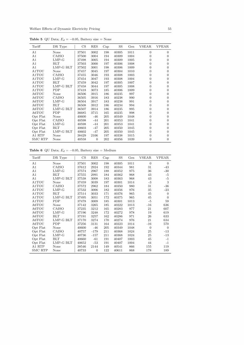
Welfare Effects of Dynamic Electricity Pricing 55
Table 5 QU Data; Ed = −0.05, Battery size = None
Tariff DR Type CS RES Cap SS Gen VSEAR VPEAR
A1 None 37501 3002 198 40305 1011 0 0A1 CAISO 37500 3004 194 40309 1004 0 0A1 LMP-G 37498 3005 194 40309 1005 0 0A1 BLT 37503 3000 197 40306 1008 0 0A1 LMP-G BLT 37502 3001 198 40306 1009 0 0A1TOU None 37457 3045 197 40304 1010 0 0A1TOU CAISO 37455 3046 193 40308 1003 0 0A1TOU LMP-G 37454 3047 193 40308 1004 0 0A1TOU BLT 37459 3042 197 40305 1007 0 0A1TOU LMP-G BLT 37458 3044 197 40305 1008 0 0A1TOU PDP 37418 3073 185 40306 1009 0 0A6TOU None 36506 3915 186 40235 997 0 0A6TOU CAISO 36505 3916 183 40238 990 0 0A6TOU LMP-G 36504 3917 183 40238 991 0 0A6TOU BLT 36508 3912 186 40234 994 0 0A6TOU LMP-G BLT 36507 3914 186 40235 995 0 0A6TOU PDP 36685 3715 165 40235 998 0 0Opt Flat None 40600 -46 205 40349 1048 0 0Opt Flat CAISO 40598 -44 201 40353 1041 0 0Opt Flat LMP-G 40598 -44 201 40353 1041 0 0Opt Flat BLT 40603 -47 205 40350 1045 0 0Opt Flat LMP-G BLT 40602 -47 205 40350 1045 0 0A1 RTP None 38429 2106 197 40338 1015 0 0SMC RTP None 40558 0 202 40356 1039 0 0
Table 6 QU Data; Ed = −0.05, Battery size = Medium
Tariff DR Type CS RES Cap SS Gen VSEAR VPEAR
A1 None 37501 3002 198 40305 1011 0 0A1 CAISO 37612 2924 192 40344 981 31 -43A1 LMP-G 37574 2967 188 40352 975 36 -30A1 BLT 37555 2991 184 40362 968 43 -5A1 LMP-G BLT 37538 3008 183 40363 968 43 -5A1TOU None 37459 3039 197 40301 1014 -3 3A1TOU CAISO 37572 2962 184 40350 980 31 -36A1TOU LMP-G 37532 3006 182 40356 976 35 -23A1TOU BLT 37514 3033 171 40376 965 45 0A1TOU LMP-G BLT 37495 3051 172 40375 965 45 0A1TOU PDP 37478 3009 185 40301 1013 -5 59A6TOU None 37142 3265 185 40222 1013 -16 636A6TOU CAISO 37235 3212 165 40283 977 21 607A6TOU LMP-G 37196 3248 172 40272 978 19 619A6TOU BLT 37191 3257 162 40286 971 26 633A6TOU LMP-G BLT 37170 3274 170 40274 976 21 634A6TOU PDP 37256 3131 164 40223 1014 -16 570Opt Flat None 40600 -46 205 40349 1048 0 0Opt Flat CAISO 40757 -179 211 40368 1024 25 -13Opt Flat LMP-G 40736 -157 211 40368 1024 25 -13Opt Flat BLT 40660 -61 191 40407 1003 45 -1Opt Flat LMP-G BLT 40652 -53 191 40407 1004 44 -1A1 RTP None 38546 2144 149 40541 866 155 119SMC RTP None 40733 0 122 40611 868 178 189

56 Clay Campaigne, Maximilian Balandat, and Lillian Ratliff
Table 7 QU Data; Ed = −0.05, Battery size = Large
Tariff DR Type CS RES Cap SS Gen VSEAR VPEAR
A1 None 37502 3001 198 40305 1011 0 1A1 CAISO 37725 2767 227 40265 1027 -15 -143A1 LMP-G 37645 2863 220 40288 1009 3 -100A1 BLT 37556 2989 185 40360 969 42 -4A1 LMP-G BLT 37538 3007 183 40361 969 41 -4A1TOU None 37461 3038 197 40301 1014 -3 4A1TOU CAISO 37682 2815 205 40292 1020 -8 -123A1TOU LMP-G 37601 2908 192 40317 1006 5 -83A1TOU BLT 37513 3032 171 40374 966 44 1A1TOU LMP-G BLT 37496 3049 172 40373 966 44 1A1TOU PDP 37555 2942 108 40388 1011 -1 140A6TOU None 37842 2632 73 40401 1017 -10 1360A6TOU CAISO 38008 2476 78 40407 1011 -3 1286A6TOU LMP-G 37950 2539 76 40412 1005 3 1309A6TOU BLT 37878 2624 73 40429 988 18 1358A6TOU LMP-G BLT 37866 2636 73 40429 989 18 1358A6TOU PDP 37899 2579 55 40423 1019 -10 1252Opt Flat None 40600 -46 205 40349 1048 0 0Opt Flat CAISO 40983 -498 308 40177 1118 -68 -51Opt Flat LMP-G 40929 -443 303 40184 1116 -67 -51Opt Flat BLT 40660 -62 192 40406 1004 44 -1Opt Flat LMP-G BLT 40652 -55 192 40406 1004 44 -1A1 RTP None 38608 2180 106 40683 769 254 182SMC RTP None 40852 0 61 40791 751 297 320
Table 8 QU Data; Ed = −0.1, Battery size = None
Tariff DR Type CS RES Cap SS Gen VSEAR VPEAR
A1 None 18631 3002 198 21435 1011 0 0A1 CAISO 18634 3002 194 21443 999 0 0A1 LMP-G 18632 3005 194 21443 1001 0 0A1 BLT 18635 2999 197 21437 1001 0 0A1 LMP-G BLT 18633 3001 197 21437 1004 0 0A1TOU None 18587 3043 196 21433 1009 0 0A1TOU CAISO 18591 3043 192 21441 997 0 0A1TOU LMP-G 18588 3045 192 21441 999 0 0A1TOU BLT 18591 3039 195 21435 1000 0 0A1TOU LMP-G BLT 18590 3041 196 21435 1002 0 0A1TOU PDP 18558 3050 172 21436 1006 0 0A6TOU None 17684 3785 175 21294 983 0 0A6TOU CAISO 17688 3784 171 21301 971 0 0A6TOU LMP-G 17685 3787 172 21300 974 0 0A6TOU BLT 17688 3779 174 21293 973 0 0A6TOU LMP-G BLT 17686 3784 174 21295 977 0 0A6TOU PDP 17891 3537 133 21295 984 0 0Opt Flat None 21782 -48 213 21522 1085 0 0Opt Flat CAISO 21786 -47 209 21530 1073 0 0Opt Flat LMP-G 21785 -46 209 21530 1074 0 0Opt Flat BLT 21787 -49 212 21526 1076 0 0Opt Flat LMP-G BLT 21786 -48 212 21526 1077 0 0A1 RTP None 19569 2129 197 21501 1018 0 0SMC RTP None 21743 0 206 21537 1068 0 0

Welfare Effects of Dynamic Electricity Pricing 57
Table 9 QU Data; Ed = −0.1, Battery size = Medium
Tariff DR Type CS RES Cap SS Gen VSEAR VPEAR
A1 None 18631 3002 198 21435 1011 0 0A1 CAISO 18743 2925 192 21475 982 31 -43A1 LMP-G 18704 2968 189 21483 976 36 -30A1 BLT 18685 2991 184 21492 968 43 -5A1 LMP-G BLT 18668 3008 183 21493 968 42 -4A1TOU None 18590 3037 196 21430 1013 -3 3A1TOU CAISO 18703 2962 184 21480 980 30 -36A1TOU LMP-G 18662 3005 182 21485 976 35 -23A1TOU BLT 18644 3031 170 21504 964 45 0A1TOU LMP-G BLT 18626 3049 171 21503 964 45 0A1TOU PDP 18617 2987 172 21432 1011 -5 59A6TOU None 18318 3140 174 21284 999 -15 635A6TOU CAISO 18410 3091 154 21347 965 19 606A6TOU LMP-G 18372 3123 161 21334 966 18 618A6TOU BLT 18366 3132 152 21345 958 24 632A6TOU LMP-G BLT 18346 3147 160 21334 962 20 632A6TOU PDP 18458 2964 110 21312 1000 -15 568Opt Flat None 21782 -48 213 21522 1085 0 0Opt Flat CAISO 21942 -182 217 21544 1060 27 -13Opt Flat LMP-G 21921 -160 217 21544 1060 27 -13Opt Flat BLT 21844 -63 198 21583 1038 46 -1Opt Flat LMP-G BLT 21837 -55 198 21583 1039 46 -1A1 RTP None 19684 2168 149 21703 875 155 119SMC RTP None 21919 0 126 21792 900 181 192
Table 10 QU Data; Ed = −0.1, Battery size = Large
Tariff DR Type CS RES Cap SS Gen VSEAR VPEAR
A1 None 18632 3001 198 21435 1011 0 1A1 CAISO 18856 2769 227 21398 1029 -15 -143A1 LMP-G 18776 2865 221 21420 1010 3 -100A1 BLT 18686 2989 184 21490 969 41 -4A1 LMP-G BLT 18668 3006 183 21491 969 41 -4A1TOU None 18591 3036 196 21430 1013 -3 4A1TOU CAISO 18813 2816 205 21424 1021 -8 -123A1TOU LMP-G 18731 2908 191 21448 1007 5 -84A1TOU BLT 18644 3030 170 21503 965 44 1A1TOU LMP-G BLT 18626 3047 171 21502 966 43 1A1TOU PDP 18689 2940 98 21531 1011 -1 139A6TOU None 18984 2613 53 21543 1015 -10 1351A6TOU CAISO 19151 2458 63 21546 1010 -3 1278A6TOU LMP-G 19092 2520 57 21555 1003 3 1301A6TOU BLT 19020 2605 53 21572 986 18 1349A6TOU LMP-G BLT 19009 2616 53 21572 987 18 1349A6TOU PDP 19040 2572 51 21561 1019 -10 1248Opt Flat None 21782 -48 213 21522 1085 0 0Opt Flat CAISO 22171 -504 317 21350 1155 -66 -51Opt Flat LMP-G 22116 -448 311 21357 1153 -65 -51Opt Flat BLT 21845 -65 199 21581 1040 45 -1Opt Flat LMP-G BLT 21837 -57 199 21581 1040 45 -1A1 RTP None 19746 2206 107 21845 779 255 184SMC RTP None 22039 0 66 21973 783 303 326

58 Clay Campaigne, Maximilian Balandat, and Lillian Ratliff
Table 11 QU Data; Ed = −0.2, Battery size = None
Tariff DR Type CS RES Cap SS Gen VSEAR VPEAR
A1 None 9196 3002 198 12000 1011 0 0A1 CAISO 9207 2999 191 12015 988 0 0A1 LMP-G 9202 3004 192 12014 993 0 0A1 BLT 9205 2994 195 12005 987 0 0A1 LMP-G BLT 9202 3000 196 12006 993 0 0A1TOU None 9153 3038 195 11996 1007 0 0A1TOU CAISO 9164 3035 188 12011 984 0 0A1TOU LMP-G 9159 3041 190 12010 989 0 0A1TOU BLT 9162 3030 192 12001 983 0 0A1TOU LMP-G BLT 9158 3036 193 12002 990 0 0A1TOU PDP 9143 3006 147 12002 1002 0 0A6TOU None 8345 3524 152 11717 955 0 0A6TOU CAISO 8356 3519 145 11731 932 0 0A6TOU LMP-G 8349 3527 148 11728 939 0 0A6TOU BLT 8355 3509 145 11718 931 0 0A6TOU LMP-G BLT 8349 3522 151 11720 941 0 0A6TOU PDP 8600 3259 87 11772 962 0 0Opt Flat None 12452 -51 228 12173 1159 0 0Opt Flat CAISO 12463 -53 221 12189 1136 0 0Opt Flat LMP-G 12461 -51 222 12189 1138 0 0Opt Flat BLT 12462 -51 225 12185 1136 0 0Opt Flat LMP-G BLT 12460 -50 226 12185 1139 0 0A1 RTP None 10154 2173 196 12132 1025 0 0SMC RTP None 12418 0 215 12203 1125 0 0
Table 12 QU Data; Ed = −0.2, Battery size = Medium
Tariff DR Type CS RES Cap SS Gen VSEAR VPEAR
A1 None 9196 3002 198 12000 1011 0 0A1 CAISO 9309 2927 193 12043 983 30 -43A1 LMP-G 9270 2970 189 12050 977 36 -30A1 BLT 9250 2990 184 12056 967 42 -4A1 LMP-G BLT 9233 3008 183 12058 968 42 -4A1TOU None 9155 3032 195 11993 1011 -3 3A1TOU CAISO 9269 2960 183 12046 981 30 -36A1TOU LMP-G 9228 3003 181 12051 975 34 -23A1TOU BLT 9210 3026 169 12067 962 44 0A1TOU LMP-G BLT 9191 3044 170 12066 962 44 0A1TOU PDP 9202 2945 137 12010 1006 -4 59A6TOU None 8976 2895 149 11721 970 -13 632A6TOU CAISO 9064 2856 132 11788 942 17 604A6TOU LMP-G 9028 2881 139 11770 941 17 615A6TOU BLT 9019 2886 132 11773 933 22 629A6TOU LMP-G BLT 9002 2901 138 11765 936 19 630A6TOU PDP 9124 2833 86 11871 984 -14 566Opt Flat None 12452 -51 228 12173 1159 0 0Opt Flat CAISO 12618 -188 229 12201 1132 31 -13Opt Flat LMP-G 12595 -165 229 12201 1131 31 -13Opt Flat BLT 12519 -67 212 12239 1109 50 -1Opt Flat LMP-G BLT 12510 -59 212 12239 1109 50 -1A1 RTP None 10265 2217 150 12332 894 156 120SMC RTP None 12594 0 136 12459 965 186 198

Welfare Effects of Dynamic Electricity Pricing 59
Table 13 QU Data; Ed = −0.2, Battery size = Large
Tariff DR Type CS RES Cap SS Gen VSEAR VPEAR
A1 None 9197 3001 198 12000 1011 0 1A1 CAISO 9422 2775 228 11969 1032 -15 -143A1 LMP-G 9342 2869 221 11989 1012 3 -100A1 BLT 9251 2989 184 12055 969 41 -4A1 LMP-G BLT 9233 3006 183 12056 969 41 -4A1TOU None 9157 3032 195 11993 1011 -3 4A1TOU CAISO 9380 2818 204 11994 1023 -8 -123A1TOU LMP-G 9297 2909 190 12016 1007 5 -84A1TOU BLT 9209 3026 169 12066 964 43 1A1TOU LMP-G BLT 9192 3043 170 12065 964 43 1A1TOU PDP 9257 2944 97 12103 1011 -1 139A6TOU None 9564 2602 46 12120 1016 -11 1335A6TOU CAISO 9732 2449 57 12125 1012 -3 1262A6TOU LMP-G 9673 2511 50 12135 1005 2 1285A6TOU BLT 9600 2593 45 12148 986 18 1332A6TOU LMP-G BLT 9589 2605 46 12148 987 17 1333A6TOU PDP 9618 2571 46 12142 1021 -10 1240Opt Flat None 12452 -51 228 12173 1159 0 0Opt Flat CAISO 12851 -515 333 12003 1228 -62 -51Opt Flat LMP-G 12795 -458 327 12010 1226 -61 -51Opt Flat BLT 12519 -69 213 12237 1111 48 -1Opt Flat LMP-G BLT 12511 -61 213 12237 1111 48 -1A1 RTP None 10327 2256 110 12473 800 258 186SMC RTP None 12718 0 76 12641 847 314 337
Table 14 QU Data; Ed = −0.3, Battery size = None
Tariff DR Type CS RES Cap SS Gen VSEAR VPEAR
A1 None 6051 3002 198 8855 1011 0 0A1 CAISO 6069 2996 187 8877 978 0 0A1 LMP-G 6062 3004 190 8876 985 0 0A1 BLT 6066 2989 188 8868 975 0 0A1 LMP-G BLT 6060 2999 194 8865 983 0 0A1TOU None 6009 3034 193 8849 1006 0 0A1TOU CAISO 6027 3027 183 8871 973 0 0A1TOU LMP-G 6019 3036 186 8869 980 0 0A1TOU BLT 6024 3020 183 8861 969 0 0A1TOU LMP-G BLT 6018 3031 190 8858 979 0 0A1TOU PDP 6018 2961 121 8858 997 0 0A6TOU None 5296 3263 128 8430 926 0 0A6TOU CAISO 5314 3257 119 8452 897 0 0A6TOU LMP-G 5303 3267 125 8446 906 0 0A6TOU BLT 5311 3240 117 8434 892 0 0A6TOU LMP-G BLT 5302 3260 126 8436 905 0 0A6TOU PDP 5549 3141 82 8607 948 0 0Opt Flat None 9412 -54 243 9115 1233 0 0Opt Flat CAISO 9430 -60 233 9138 1199 0 0Opt Flat LMP-G 9427 -56 234 9138 1202 0 0Opt Flat BLT 9427 -54 235 9138 1197 0 0Opt Flat LMP-G BLT 9425 -52 238 9135 1200 0 0A1 RTP None 7029 2217 194 9052 1033 0 0SMC RTP None 9382 0 223 9159 1182 0 0

60 Clay Campaigne, Maximilian Balandat, and Lillian Ratliff
Table 15 QU Data; Ed = −0.3, Battery size = Medium
Tariff DR Type CS RES Cap SS Gen VSEAR VPEAR
A1 None 6051 3002 198 8855 1011 0 0A1 CAISO 6165 2930 193 8901 985 30 -43A1 LMP-G 6125 2971 189 8907 978 35 -30A1 BLT 6105 2990 184 8911 967 41 -4A1 LMP-G BLT 6088 3007 183 8912 967 41 -4A1TOU None 6011 3028 193 8846 1009 -3 3A1TOU CAISO 6126 2959 182 8903 981 30 -36A1TOU LMP-G 6085 3001 180 8906 975 34 -23A1TOU BLT 6065 3022 168 8919 960 44 0A1TOU LMP-G BLT 6047 3040 169 8918 961 43 0A1TOU PDP 6074 2924 97 8902 1004 -4 58A6TOU None 5920 2672 118 8474 942 -11 628A6TOU CAISO 6004 2643 107 8540 921 15 602A6TOU LMP-G 5971 2660 113 8518 917 16 612A6TOU BLT 5959 2663 109 8513 908 20 625A6TOU LMP-G BLT 5945 2677 112 8509 911 19 626A6TOU PDP 6040 2726 80 8685 970 -13 565Opt Flat None 9412 -54 243 9115 1233 0 0Opt Flat CAISO 9584 -194 242 9147 1203 34 -13Opt Flat LMP-G 9560 -170 242 9148 1203 34 -13Opt Flat BLT 9483 -71 226 9186 1179 53 -1Opt Flat LMP-G BLT 9474 -63 226 9185 1179 53 -1A1 RTP None 7136 2265 153 9249 914 157 121SMC RTP None 9560 0 146 9414 1029 192 204
Table 16 QU Data; Ed = −0.3, Battery size = Large
Tariff DR Type CS RES Cap SS Gen VSEAR VPEAR
A1 None 6052 3001 198 8855 1011 0 1A1 CAISO 6278 2780 228 8830 1035 -15 -143A1 LMP-G 6197 2872 221 8848 1014 3 -100A1 BLT 6106 2988 184 8910 968 40 -4A1 LMP-G BLT 6088 3006 183 8911 969 40 -4A1TOU None 6012 3027 193 8847 1009 -3 4A1TOU CAISO 6236 2820 203 8853 1025 -9 -123A1TOU LMP-G 6154 2909 189 8873 1008 4 -84A1TOU BLT 6065 3021 168 8919 962 43 1A1TOU LMP-G BLT 6047 3039 168 8917 962 42 1A1TOU PDP 6113 2947 97 8964 1012 -1 139A6TOU None 6430 2592 45 8977 1016 -11 1318A6TOU CAISO 6599 2443 56 8986 1015 -3 1245A6TOU LMP-G 6540 2504 49 8995 1007 2 1268A6TOU BLT 6467 2583 45 9005 986 17 1315A6TOU LMP-G BLT 6455 2595 45 9005 987 17 1316A6TOU PDP 6482 2575 46 9011 1025 -11 1233Opt Flat None 9412 -54 243 9115 1233 0 0Opt Flat CAISO 9821 -526 346 8948 1301 -58 -51Opt Flat LMP-G 9763 -467 341 8955 1299 -58 -51Opt Flat BLT 9483 -74 226 9183 1181 51 -1Opt Flat LMP-G BLT 9474 -65 226 9183 1181 51 -1A1 RTP None 7199 2307 113 9392 821 261 188SMC RTP None 9686 0 87 9600 910 324 348
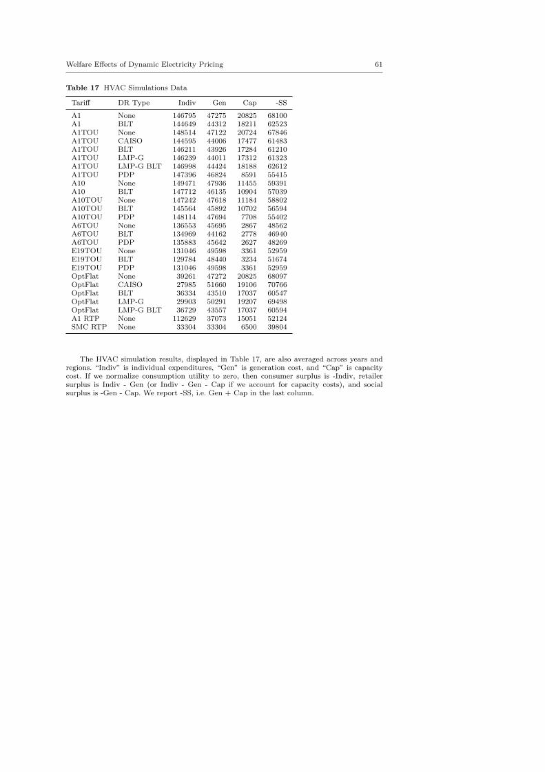
Welfare Effects of Dynamic Electricity Pricing 61
Table 17 HVAC Simulations Data
Tariff DR Type Indiv Gen Cap -SS
A1 None 146795 47275 20825 68100A1 BLT 144649 44312 18211 62523A1TOU None 148514 47122 20724 67846A1TOU CAISO 144595 44006 17477 61483A1TOU BLT 146211 43926 17284 61210A1TOU LMP-G 146239 44011 17312 61323A1TOU LMP-G BLT 146998 44424 18188 62612A1TOU PDP 147396 46824 8591 55415A10 None 149471 47936 11455 59391A10 BLT 147712 46135 10904 57039A10TOU None 147242 47618 11184 58802A10TOU BLT 145564 45892 10702 56594A10TOU PDP 148114 47694 7708 55402A6TOU None 136553 45695 2867 48562A6TOU BLT 134969 44162 2778 46940A6TOU PDP 135883 45642 2627 48269E19TOU None 131046 49598 3361 52959E19TOU BLT 129784 48440 3234 51674E19TOU PDP 131046 49598 3361 52959OptFlat None 39261 47272 20825 68097OptFlat CAISO 27985 51660 19106 70766OptFlat BLT 36334 43510 17037 60547OptFlat LMP-G 29903 50291 19207 69498OptFlat LMP-G BLT 36729 43557 17037 60594A1 RTP None 112629 37073 15051 52124SMC RTP None 33304 33304 6500 39804
The HVAC simulation results, displayed in Table 17, are also averaged across years andregions. “Indiv” is individual expenditures, “Gen” is generation cost, and “Cap” is capacitycost. If we normalize consumption utility to zero, then consumer surplus is -Indiv, retailersurplus is Indiv - Gen (or Indiv - Gen - Cap if we account for capacity costs), and socialsurplus is -Gen - Cap. We report -SS, i.e. Gen + Cap in the last column.

62 Clay Campaigne, Maximilian Balandat, and Lillian Ratliff
References
B. R. Alexander. Dynamic pricing? Not so fast! A residential consumer perspective. ElectricityJournal, 23(6):39–49, 2010. ISSN 10406190. doi: 10.1016/j.tej.2010.05.014.
A. Aswani, N. Master, J. Taneja, V. Smith, A. Krioukov, D. Culler, and C. Tomlin. Identify-ing models of HVAC systems using semiparametric regression. In 2012 American ControlConference (ACC), pages 3675–3680, 2012. ISBN 9781457710964. doi: 10.1109/ACC.2012.6315566. URL http://ieeexplore.ieee.org/lpdocs/epic03/wrapper.htm?arnumber=6315566.
M. Balandat, F. Oldewurtel, M. Chen, and C. J. Tomlin. Contract design for frequencyregulation by aggregations of commercial buildings. In Communication, Control, andComputing (Allerton), 52nd Annual Allerton Conference on, pages 38–45, 2014. doi:http://doi.org/10.1109/ALLERTON.2014.7028433. URL http://ieeexplore.ieee.org/xpl/articleDetails.jsp?arnumber=7028433.
M. Balandat, C. Campaigne, and L. Ratliff. The pyDR python package, Aug 2016a. URLhttps://github.com/Balandat/pyDR. GitHub repository.
M. Balandat, C. Campaigne, and L. Ratliff. Data for pyDR simulations, Aug 2016b. URLhttps://www.ocf.berkeley.edu/~balandat/pyDR_data.zip.
B. Bollinger and W. R. Hartmann. Welfare effects of home automation technology with dy-namic pricing. Working Paper, April 2015.
J. Boomhower and L. W. Davis. Do Energy Efficiency Investments Deliver at the Right Time?2016. URL http://ei.haas.berkeley.edu/research/papers/WP271.pdf.
S. Borenstein. The Long-Run Efficiency of Real Time Electricity Pricing. The Energy Journal,26:93–116, 2005. ISSN 01956574. doi: 10.5547/ISSN0195-6574-EJ-Vol26-No3-5.
S. Borenstein. Time-varying retail electricity prices: Theory and practice. In J. M. Griffinand S. L. Puller, editors, Electricity deregulation: choices and challenges. The University ofChicago Press, 2009. ISBN 9780226308586.
S. Borenstein. Peak-Time Rebates: Money for Nothing?, 2014. URL http://www.greentechmedia.com/articles/read/Peak-Time-Rebates-Money-for-Nothing.
S. Borenstein. The Economics of Fixed Cost Recovery by Utilities. 2016. URL https://ei.haas.berkeley.edu/research/papers/WP272.pdf.
S. Borenstein and S. Holland. On the efficiency of competitive electricity markets with time-invariant retail prices. The Rand Journal of Economics, 36(3):469–493, 2005. ISSN 07416261.doi: Article. URL http://www.nber.org/papers/w9922.
S. Borenstein and S. P. Holland. On the Efficiency of Competitive Electricity Markets WithTime-Invariant Retail Prices. RAND Journal of Economics, 36(August):469–493, 2003.
S. Borenstein, M. Jaske, and A. R. Rosenfeld. Dynamic Pricing , Advanced Metering andDemand Response in Electricity Markets. 2002.
R. L. Borlick. Pricing Negawatts. Public Utilities Fortnightly, 14:148, 2010.R. L. Borlick, J. Bowring, J. Bushnell, P. A. Centolella, H.-P. Chao, A. Faruqui, M. Giberson,
D. Gonatas, S. Harvey, B. F. Hobbs, W. W. Hogan, J. P. Kalt, R. J. Michaels, S. S. Oren,D. B. Patton, C. Pirrong, S. L. Pope, L. E. Ruff, R. Schmalensee, R. J. Shanker, V. L.Smith, and R. D. Tabors. BRIEF OF ROBERT L. BORLICK, JOSEPH BOWRING,JAMES BUSHNELL, AND 18 OTHER LEADING ECONOMISTS AS AMICI CURIAEIN SUPPORT OF PETITIONERS, 2012. URL http://www.scotusblog.com/wp-content/uploads/2015/09/2015-09-09-SCOTUS_EconomistsBriefDR.pdf.
D. B. Brown, J. E. Smith, and P. Sun. Information Relaxations and Duality in StochasticDynamic Programs. Operations Research, 58(4-Part-1):785–801, 2010. ISSN 0030-364X.doi: 10.1287/opre.1090.0796.
J. Bushnell, B. F. Hobbs, and F. a. Wolak. When It Comes to Demand Response, Is FERC ItsOwn Worst Enemy? Electricity Journal, 22(8):9–18, 2009a. ISSN 10406190. doi: 10.1016/j.tej.2009.08.004.
J. Bushnell, B. F. Hobbs, and F. A. Wolak. When It Comes to Demand Response, Is FERCIts Own Worst Enemy? Electricity Journal, 22(8):9–18, 2009b. ISSN 10406190. doi: 10.1016/j.tej.2009.08.004.
CAISO. Fifth replacement ferc electric tariff, July 2015. URL https://www.caiso.com/Documents/ConformedTariff_Jun12_2015.pdf.
California Department of Water Resources. California Irrigation Management System, 2015.URL http://www.cimis.water.ca.gov/.

Welfare Effects of Dynamic Electricity Pricing 63
California Independent System Operator Corporation. Load granularity refinements issuepaper and pricing analysis study. Presentation, Aug 2013. URL https://www.caiso.com/Documents/Presentation-LoadGranularityRefinementsIssuePaperAug21_2013.pdf.
California Independent System Operator Corporation. Interface Specificationfor OASIS, 4.2.6 edition, Mar 2015. URL http://www.caiso.com/Documents/OASIS-InterfaceSpecification_v4_2_6Clean_Independent2015Release.pdf.
California State Senate. Senate bill no. 1122, Sep 2012. URL https://leginfo.legislature.ca.gov/faces/billTextClient.xhtml?bill_id=201120120SB1122.
D. Callaway, M. Fowlie, and G. McCormick. Location, location, location: The variable valueof renewable energy and demand-side efficiency resources. 2015. URL https://ei.haas.berkeley.edu/research/papers/WP264.pdf.
H.-P. Chao and M. DePillis. Incentive effects of paying demand response in wholesale electricitymarkets. Journal of Regulatory Economics, 43:265–283, 2013. ISSN 0922-680X. doi: 10.1007/s11149-012-9208-1. URL http://link.springer.com/10.1007/s11149-012-9208-1\nhttp://link.springer.com/article/10.1007/s11149-012-9208-1.
Z. Chen, L. Wu, and Y. Fu. Real-time price-based demand response management for residentialappliances via stochastic optimization and robust optimization. IEEE Transactions onSmart Grid, 3(4):1822–1831, Dec 2012. ISSN 1949-3053. doi: 10.1109/TSG.2012.2212729.
K. Coughlin, M. A. Piette, C. Goldman, and S. Kiliccote. Estimating Demand Response LoadImpacts: Evaluation of Baseline Load Models for Non- Residential Buildings in California.2008.
M. A. Crew, C. S. Fernando, and P. R. Kleindorfer. The theory of peak-load pricing: Asurvey. Journal of Regulatory Economics, 8(3):215–248, 1995. ISSN 1573-0468. doi: 10.1007/BF01070807. URL http://dx.doi.org/10.1007/BF01070807.
D. Cullenward and A. Coghlan. Structural oversupply and credibility in California’s carbonmarket. Electricity Journal, 29(5):7–14, 2016. ISSN 10406190. doi: 10.1016/j.tej.2016.06.006.
B. Defourny, D. Ernst, and L. Wehenkel. Multistage Stochastic Programming. In DecisionTheory Models for Applications in Artificial Intelligence, pages 97–143. IGI Global, 2011.doi: 10.4018/978-1-60960-165-2.ch006.
Q. Dong, L. Yu, W. Z. Song, L. Tong, and S. Tang. Distributed demand and response algorithmfor optimizing social-welfare in smart grid. In Parallel Distributed Processing Symposium(IPDPS), 2012 IEEE 26th International, pages 1228–1239, May 2012. doi: 10.1109/IPDPS.2012.112.
G. Fagilde. HVAC by the Numbers: How to Save by Cutting Waste. URL https://www.pge.com/en/mybusiness/save/smbblog/article/HVACnumbers.page.
A. Faruqui. The global movement toward cost-reflective tariffs (presentation), 2015.URL http://www.brattle.com/system/publications/pdfs/000/005/172/original/The_global_movement_toward_cost-reflective_tariffs__Faruqui_EUCI.pdf?1431628764.
A. Faruqui, R. Hledik, and J. Palmer. Time-Varying and Dynamic Rate Design. 2012.M. Fowlie. Time to Unleash the Carbon Market?, 2016. URL https://energyathaas.
wordpress.com/2016/06/20/time-to-unleash-the-carbon-market/.J. Gannon, D. Brooks, L. Chow, and S. Brant. The 2013 2014 Resource Adequacy Report.
Technical Report August, The California Public Utilities Commission, 2015. URL http://www.cpuc.ca.gov/ra/.
R. Gondhalekar, F. Oldewurtel, and C. N. Jones. Least-restrictive robust periodic modelpredictive control applied to room temperature regulation. Automatica, 49(9):2760 – 2766,2013. ISSN 0005-1098. doi: http://dx.doi.org/10.1016/j.automatica.2013.05.009. URL http://www.sciencedirect.com/science/article/pii/S0005109813002793.
Gurobi Optimization. Gurobi Optimizer Reference Manual, 2016. URL http://www.gurobi.com.
A. C. Harberger. The Measurement of Waste. The American Economic Review, 54(3):58–76,1964.
M. Harding and C. Lamarche. Empowering consumers through data and smart technology:Experimental evidence on the consequences of time-of-use electricity pricing policies. Journalof Policy Analysis and Management, 35(4):906–931, 2016. ISSN 1520-6688. doi: 10.1002/pam.21928. URL http://dx.doi.org/10.1002/pam.21928.
T. Hatta and J. Haltiwanger. Tax Reform and Strong Substitutes. 1984.K. Herter and S. Wayland. Residential response to critical-peak pricing of electricity: Califor-
nia evidence. Energy, 35(4):1561 – 1567, 2010. ISSN 0360-5442. doi: http://dx.doi.org/10.1016/j.energy.2009.07.022. URL http://www.sciencedirect.com/science/article/pii/

64 Clay Campaigne, Maximilian Balandat, and Lillian Ratliff
S0360544209003016. Demand Response Resources: the {US} and International Experi-enceDemand Response Resources: the {US} and International Experience.
W. W. Hogan. Demand response pricing in organized wholesale markets. Demand ResponseCompensation in Organized Wholesale Energy Markets, 2010. URL http://www.hks.harvard.edu/fs/whogan/Hogan_IRC_DR_051310.pdf.
W. W. Hogan. Time of Use Rates and Real Time Prices. 2014. URL http://www.hks.harvard.edu/fs/whogan/Hogan_TOU_RTP_Newark_082314.pdf.
K. Hsia-Kiung, E. Reyna, and T. O’Connor. Carbon Market California: a comprehensiveanalysis of the Golden State’s cap-and-trade program: Year One: 2012-2013. 2014. URLhttp://www.edf.org/sites/default/files/content/ca-cap-and-trade_1yr_22_web.pdf.
J. E. Hughes and M. Podolefsky. Getting Green with Solar Subsidies: Evidence from theCalifornia Solar Initiative. Journal of the Association of Environmental and ResourceEconomists, 2(2):235–275, 2015. ISSN 23335955. doi: 10.1086/681131.
Interagency Working Group on Social Cost of Carbon. Technical Update of the SocialCost of Carbon for Regulatory Impact Analysis Under Executive Order 12866. 2013.URL https://www.whitehouse.gov/sites/default/files/omb/inforeg/social_cost_of_carbon_for_ria_2013_update.pdf.
K. Ito. Do Consumers Respond to Marginal or Average Price? Evidence from NonlinearElectricity Pricing. American Economic Review, 104(2):537–563, feb 2014. ISSN 0002-8282. doi: 10.1257/aer.104.2.537. URL http://dx.doi.org/10.1257/aer.104.2.537http://pubs.aeaweb.org/doi/10.1257/aer.104.2.537.
M. R. Jacobsen, C. R. Knittel, J. M. Sallee, and A. A. V. Benthem. Sufficient Statisticsfor Imperfect Externality-Correcting Policies. 2016. URL http://www.nber.org/papers/w22063.
P. Joskow and J. Tirole. Retail Electricity Competition. RAND Journal of Economics, 37:799–815, 2006. ISSN 07416261. doi: 10.1111/j.1756-2171.2006.tb00058.x.
A. Mesbah. Stochastic model predictive control: An overview and perspectives for futureresearch. IEEE Control Systems Magazine, 2016. Accepted.
J. Migden-Ostrander, B. Watson, D. Lamont, and R. Sedano. Decoupling Case Studies: Rev-enue Regulation Implementation in Six States. Technical report, The Regulatory AssistanceProject, Montpelier, VT, 2014. URL http://www.raponline.org/document/download/id/7209.
J. Neubauer and M. Simpson. Deployment of Behind-The-Meter Energy Storage for DemandCharge Reduction. 2015. URL http://www.nrel.gov/docs/fy15osti/63162.pdf.
F. Oldewurtel, T. Borsche, M. Bucher, P. Fortenbacher, M. G. V. T. Haring, J. L. Math-ieu, O. Megel, E. Vrettos, and G. Andersson. A framework for and assessment of de-mand response and energy storage in power systems. In Proceedings of IREP Symposium:Bulk Power System Dynamics and Control - IX Optimization, Security and Control of theEmerging Power Grid, IREP 2013, 2013. ISBN 9781479901999. doi: 10.1109/IREP.2013.6629419.
Pacific Gas and Electric Company. Non-residential rates, a.Pacific Gas and Electric Company. PG&E Tariff Book, b. URL https://www.pge.com/
tariffs/ERS.SHTML.Pacific Gas and Electric Company. Peak Day Pricing Fact Sheet: Dual Par-
ticipation for Peak Day Pricing, 2011. URL http://www.pge.com/includes/docs/pdfs/mybusiness/energysavingsrebates/demandresponse/peakdaypricing/PDPDualParticipationCustFactSheet.pdf.
Pacific Gas and Electric Company. Understanding energy use and prices, July 2016a. URLhttp://www.pge.com/tariffs/energy_use_prices.shtml.
Pacific Gas and Electric Company. Electric Rates for Commercial/General Service (A-1, A-6,A-10, E-19), Jan 2016b. URL https://www.pge.com/tariffs/Comml_160101-160229.xls.
Pacific Gas and Electric Company. SmartRate FAQ, Aug 2016c. URL https://www.pge.com/en_US/residential/rate-plans/rate-plan-options/smart-rate-add-on/discover-smart-rate/discover-smart-rate.page?
Pacific Gas and Electric Company. Renewable feed-in tariffs, 2016d. URL https://www.pge.com/en_US/for-our-business-partners/floating-pages/renewable-feed-in-tariffs/renewable-feed-in-tariffs.page.
J. P. Pfeifenberger, K. Spees, and S. A. Newell. Resource Adequacy in California. Tech-nical Report October, Brattle Group, 2012. URL http://www.brattle.com/system/publications/pdfs/000/004/827/original/Resource_Adequacy_in_California_Calpine_
Welfare Effects of Dynamic Electricity Pricing 65
Pfeifenberger_Spees_Newell_Oct_2012.pdf.W. B. Powell. Approximate Dynamic Programming: Solving the curses of dimensionality. John
Wiley & Sons, 2nd edition, 2011.pvlib. pvlib python library, 2016. URL https://github.com/pvlib/pvlib-python.P. Samadi, H. Mohsenian-Rad, R. Schober, and V. W. S. Wong. Advanced demand side
management for the future smart grid using mechanism design. IEEE Transactions onSmart Grid, 3(3):1170–1180, Sept 2012. ISSN 1949-3053. doi: 10.1109/TSG.2012.2203341.
R. J. Shanker. COMMENTS OF ROY J. SHANKER PH.D. REGARDING THE EN-ERGY MARKET DEMAND RESPONSE NOPR ON BEHALF OF THE PJM POWERPROVIDERS (P3). Technical report, Docket No. RM10-17-000, 2010.
W. Shi and V. W. S. Wong. Real-time vehicle-to-grid control algorithm under price uncertainty.In Smart Grid Communications (SmartGridComm), 2011 IEEE International Conferenceon, pages 261–266, Oct 2011. doi: 10.1109/SmartGridComm.2011.6102330.
K. Singh, N. P. Padhy, and J. Sharma. Influence of price responsive demand shifting biddingon congestion and lmp in pool-based day-ahead electricity markets. IEEE Transactions onPower Systems, 26(2):886–896, May 2011. ISSN 0885-8950. doi: 10.1109/TPWRS.2010.2070813.
J. N. Tsitsiklis and Y. Xu. Pricing of fluctuations in electricity markets. European Journal ofOperational Research, 246(1):199–208, 2015. ISSN 03772217. doi: 10.1016/j.ejor.2015.04.020. URL http://www.sciencedirect.com/science/article/pii/S0377221715003136.
K. M. Tsui and S. C. Chan. Demand response optimization for smart home scheduling underreal-time pricing. IEEE Transactions on Smart Grid, 3(4):1812–1821, Dec 2012. ISSN1949-3053. doi: 10.1109/TSG.2012.2218835.
U.S. Department of Energy. Buildings Energy Data Book: Building Sector Energy Consump-tion. URL http://buildingsdatabook.eren.doe.gov/TableView.aspx?table=1.1.9.
U.S. Energy Information Administration. State Energy Data System. URL http://www.eia.gov/state/seds/#.
J. S. Vardakas, N. Zorba, and C. V. Verikoukis. A survey on demand response programs insmart grids: Pricing methods and optimization algorithms. IEEE Communications SurveysTutorials, 17(1):152–178, Firstquarter 2015. ISSN 1553-877X. doi: 10.1109/COMST.2014.2341586.
F. A. Wolak, J. Bushnell, and B. F. Hobbs. The California ISO’s Proxy Demand Resource(PDR) Proposal. Technical report, Market Surveillance Committee of the California ISO,2009. URL http://www.caiso.com/239f/239fc54917610.pdf.
A. Wright. Maximum Demand Indicator, 1902. URL https://www.google.com/patents/US702846.
L. Xu. Demand response net benefits test. Technical report, California Independent SystemOperator Corporation, Jul 2011. URL http://www.caiso.com/Documents/FinalProposal_Appendix-DemandResponseNetBenefitsTest.pdf.
P. Yang, G. Tang, and A. Nehorai. A game-theoretic approach for optimal time-of-use elec-tricity pricing. IEEE Transactions on Power Systems, 28(2):884–892, May 2013. ISSN0885-8950. doi: 10.1109/TPWRS.2012.2207134.
V. M. Zavala. Real-time optimization strategies for building systems. Industrial & EngineeringChemistry Research, 52(9):3137–3150, 2013. doi: 10.1021/ie3008727. URL http://dx.doi.org/10.1021/ie3008727.
M. Zugno, J. M. Morales, P. Pinson, and H. Madsen. A bilevel model for electricity retailers’participation in a demand response market environment. Energy Economics, 36(0):182– 197, 2013. ISSN 0140-9883. doi: http://dx.doi.org/10.1016/j.eneco.2012.12.010. URLhttp://www.sciencedirect.com/science/article/pii/S0140988312003477.