Welfare Impacts of Rising Food Prices: Evidence from India

by Regine Weber

Center for Development Research (ZEF), University of Bonn

Abstract.

India has been experiencing rising food prices during the last five years. In this

paper we explore how inflationary food prices impact India’s consumer welfare

and poverty ratios, by calculating the compensating variation as a welfare

measure. We account for changes in consumption patterns, i.e. substitution effects

among food items, by including own and cross price elasticities obtained through

the estimation of a demand system, i.e. QUAIDS. Our results show that consumers

substitute high value commodities, e.g. milk, livestock products and fruits in case of

rising prices. Moreover, a 10 per cent price increase on average causes a welfare

loss of 5 to 6 per cent of monthly income in rural areas and 3 to 4 per cent welfare

loss in urban areas. As a result, there is a drop below the poverty line of an

additional 4.69 per cent and 2.19 per cent of households in rural and urban regions

respectively.

Keywords: QUAIDS, compensating variation, welfare impacts, poverty dynamics.

JEL codes: I32, Q18

1

1. Introduction

India has been experiencing inflationary food prices during the last five years. The prices of all

major food commodities have been increasing by 10 per cent since 2008/09 (Mishra and Roy

2012). Figure 1 shows the development of the Indian wholesale price index of various food prices

from 2005 to 2014. Food prices started to increase at a faster pace in mid-2009 and are rising and

experiencing strong spikes until today. Initially, the Indian food price inflation was led by cereals

(Ganguli and Gulati 2013). However, in 2011-12 and 2013-14 food inflation has shifted to high

value commodities, like milk, milk products, fruits and vegetables (Gulati and Saini 2014). This

is a rather problematic development, since these goods are major protein and vitamin sources.

Hence, they play a key role in nutrition security and are of particular importance in a diversified

and balanced diet (Gulati and Saini 2014).

The persistent rise in food prices is of particular concern for India, where one third of the

population is considered poor (Gulati, Gujra and Nandakumar et al. 2012) and the average Indian

household spends half of its income on food. High food prices are most likely to affect the

poorest of the society, as poor people spend a larger share of their income on food (Robles and

Keefe 2011). In 2012, 17 percent of India’s population was undernourished (World Bank 2014)

and 46 per cent of children under three were underweight (Menon 2013). Hence, persistently high

food prices potentially threaten India’s food security and are likely to cause further

impoverishment and hunger.

Food security, particularly access to food, has been a longstanding political goal of the Indian

government, which has been running an extensive, cereals based targeted public distribution

scheme (TPDS) for consumers since 1997 (Jha and Srinivasan 2004, Saini and Kozicka 2014). In

2013, India introduced the National Food Security Act (NFSA), converting the right to food into

a legal entitlement and granting food subsidies on staple commodities to 75 per cent of its rural

and 50 per cent of its urban population (Mishra 2013). This amounts to a total of around 800

million beneficiaries, or two thirds of India’s population of 1.2 billion (Mishra 2013). The NFSA

requires an estimated 61.2 million tons of grains per year and is estimated to cost India as much

as 0.7 per cent of its gross domestic product each year (Mishra 2013, Kozicka et al. 2015). The

focus of both the TPDS and the NFSA is on grains. Hence, both measures address food security

by increasing the calorie intake and the quantity of food available, while ignoring the importance

of micronutrient deficiencies as cause of malnutrition (Kotwal, Ramaswami and Murugkar 2011).

2

Hence, both programs grant access to basic staple commodities, while not accounting for

nutrition security.

In this paper, we1 aim to analyze the welfare impact of India’s food price inflation on its

consumers. De Janvry and Sadoulet (2009) quantify in their paper the impact of rising food prices

on Indian households by estimating the compensating variation as the percentage change in

household expenditure after a simulated international food price increase in cereals and edible

oils. Their results inter alia identify the rural poor non-farming households as the main welfare

losers, followed by marginal farmers and urban poor. These results invalidate the classic

suggestion of the urban poor as biggest welfare losers of a food price increase. Their study

focuses on first round effects and excludes substitution effects among goods. Hence they do not

account for a change in the consumer’s consumption pattern.

The objective of the present study is to explore to what magnitude inflationary food prices impact

India’s consumer welfare and poverty ratios. We consider changes in consumption patterns, i.e.

substitution effects among food items by including own and cross price elasticities obtained

through the estimation of a demand system. Our work is similar to that of Robles and Torero

(2010), who estimate the welfare impact and poverty dynamics of rising food prices on

consumers in a selection of Latin American countries, incorporating substitution effects among

food items.

The paper is structured as follows: We start with a data description of the 68th

round of the Indian

National Sample Survey on Household Expenditure. Our empirical approach consists of two

steps: a demand system estimation and subsequent welfare analysis. In a first step we estimate

Blanks, Blundell and Lewbel’s Quadratic Almost Ideal Demand System (QUAIDS) to evaluate

income and compensated own and cross price elasticities, and analyze changes in consumption

behavior after a change in food prices. Subsequently, we simulate a 10 and 20 per cent food price

increase and employ the obtained compensated own and cross price elasticities to calculate the

compensation variation as a measure of welfare loss and the impact of the simulated food price

scenarios on India’s poverty ratios. In the last chapter, we discuss our results in the context of

India’s TPDS and National Food Security Act. The study contributes to the understanding of

1 Note from the author: The use of “we” and “our” or any related term should be considered as a stylistic device. The

present study is my own work and I am the only responsible author.

3

changes in consumer behavior after a food price increase and to increasing the knowledge about

welfare impacts of high food prices on Indian consumers.

2. Data: Indian National Sample Survey of Household Expenditure

Our analysis of welfare impacts and the estimation of income and price elasticities are based on

the 68th

round of the Indian National Sample Survey (NSS) of Household Consumer Expenditure,

carried out by India’s National Sample Survey Office of the Ministry of Statistics and

Programme Implementation. The survey was conducted between July 2011 and June 2012 and

was published in July 2013. The survey is cross-sectional, representative at the national level and

based on a stratified multi-stage sampling design. Participating households are randomly selected

and report demographic data and household characteristics, consumption quantity and value, total

consumption expenditure and the value and quantity of home production.2 The quantity and value

of consumption is reported on the basis of a 30 day recall period. Additionally, a 365 day recall

period is available for selected non-food items to overcome the probability that non-food items

are consumed on an irregular basis. The survey covers a total of 151 food items and 155 non-food

items (National Sample Survey Office 2013b).

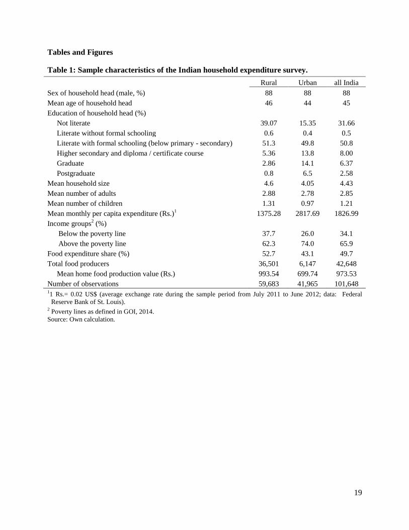
Table 1 presents the summary of household characteristics at the all India level, as well as for the

rural and urban sub-samples. As expected, the greater share of population lives in rural areas (69

percent). In 88 per cent of the households, the head is male and the majority of household heads

are literate with formal schooling; that is below primary, primary, middle and secondary school.

Nearly 40 percent of the rural and 15 percent of the urban areas comprise illiterate households.

The mean size of households is 4.6 in rural and 4.05 in urban areas, consisting on average of two

to three adults and one child.

Further, the mean monthly per capita expenditure is 1375.28 Indian Rupees (Rs.) in rural and Rs.

2817.69 in urban areas. The majority of households, 65.9 per cent, is above the poverty line

(APL). Nearly 34 per cent of India’s population has a monthly expenditure below the poverty line

(BPL) threshold, 37.7 percent in rural and 26 percent in urban areas. Consequently, rural

households spend more than half (52.7 per cent) of their monthly income on food, while

households in urban areas have a food expenditure share of 43.1 per cent. At the all India level, a

2 Since we use the household’s per capita expenditure as a proxy for income, we employ the terms expenditure and

income interchangeably in the present study.

4

comparatively high share of nearly 50 per cent of the monthly income is spent on food. Food

expenditure shares are of high importance for further analysis.

Moreover, 42 per cent of the sample households report on food production. The majority of food

producing households, 86 per cent, is allocated in rural areas and the remaining 14 per cent farm

in urban areas. Farming households produce an estimated mean production value of Rs. 993.54 in

rural and Rs. 699.74 in urban areas. Also, only 16 per cent of food producing households are net

food producers, meaning that the food production value exceeds the food consumption value.

Consequently, 84 per cent of farming households still rely on the market for their consumption.

3. Demand Analysis

3.1. Quadratic Almost Ideal Demand System

We start our modeling approach by estimating a demand system, which allows us to calculate

income elasticities and compensated own and cross price elasticities. We follow Blanks, Blundell

and Lewbel (1997) and estimate the Quadratic Almost Ideal Demand System, which is the

quadratic extension of Deaton and Muellbauer’s (1980) Almost Ideal Demand System. Blanks,

Blundell and Lewbel (1997) extended the original version to a rank three demand system with

Engle curvature flexibility, thus allowing for non-linear Engel curves. This means that goods can

be luxuries at low levels of income and basic needs at high levels of income. QUAIDS is

multistage demand system, in which the household’s total expenditure is allocated among all

goods first and then to different sub-groups of goods.

Following Blanks, Blundell and Lewbel (1997), QUAIDS is derived from the indirect utility

function of consumers, given by:

ln 𝑉 (𝐩, 𝑒) = {[ln 𝑒 − ln 𝑎(𝐩)

𝑏(𝐩)]

−1

+ 𝜆(𝐩)}

−1

(1)

where 𝑒 is the total expenditure and 𝐩 is a vector of prices, [ln𝑒 − ln𝑎(𝐩)]/𝑏(𝐩) is the indirect

utility function originating from Muellbauer’s (1976) Price Independent Generalized Logarithmic

(also known as PIGLOG) Demand System. Applying Roy’s identity to the indirect utility

function lnV(𝐩, 𝑒) yields

5

𝑠ℎ𝑖 = 𝛼𝑖 + ∑ 𝛾𝑖𝑗

𝑛

𝑗=1

ln 𝑝𝑗 + 𝛽𝑖 ln [𝑒

𝑎(𝐩)] +

𝜆𝑖

𝑏(𝐩){ln [

𝑒

𝑎(𝐩)]}

2

(2)

where 𝑠ℎ𝑖 is the household expenditure share for good 𝑖 and 𝑛 is the number of aggregate

commodity groups. Furthermore, ln 𝑎(𝐩) is a transcendental function defined as:

ln 𝑎(𝐩) = 𝛼0 + ∑ 𝛼𝑖 ln 𝑝𝑖 +

𝑛

𝑖=1

1

2∑ ∑ 𝛾𝑖𝑗

𝑛

𝑗=1

ln 𝑝𝑗 ln 𝑝𝑖

𝑛

𝑖=1

(3)

𝑏(𝐩) is the Cobb Douglas price aggregator and is homogenous of degree zero in prices:

𝑏(𝐩) = ∏ 𝑝𝑖𝛽

𝑛

𝑖=1

(4)

And 𝜆(𝐩) is a differentiable, homogeneous function of degree zero in prices:

𝜆(𝐩) = ∑ 𝜆𝑖

𝑛

𝑖=1

ln 𝑝𝑖 (5)

Due to theoretical assumptions, additional constraints on parameters must be imposed. These

constraints are adding up and homogeneity:

∑ 𝛼𝑖

𝑛

𝑖=1

= 1 ∑ 𝛽𝑖

𝑛

𝑖=1

= 0, ∑ 𝛾𝑖𝑗

𝑛

𝑖=1

= 0, ∑ 𝛾𝑖𝑗

𝑛

𝑗=1

= 0, ∑ 𝜆𝑖

𝑛

𝑖=1

= 0 (6)

As well as Slutsky symmetry:

𝛾𝑖𝑗 = 𝛾𝑗𝑖 (7)

Furthermore, expenditure shares must sum up to one:

∑ 𝑠ℎ𝑖

𝑛

𝑖=1

= 1 (8)

On the basis of the estimated demand shares 𝑠ℎ𝑖, we then compute uncompensated own and cross

price elasticities, to obtain compensated price elasticities through the Slutsky equation. Following

Jehle and Reny (2011), uncompensated or Marshallian price elasticities are given by:

6

𝜖𝑖𝑗 = 𝜕𝑠ℎ𝑖

𝜕𝑙𝑛𝑝𝑗

1

𝑠ℎ𝑖− 𝛿𝑖𝑗 (9)

where 𝛿𝑖𝑗 is Kronecker’s delta, which takes the value one when 𝑖 = 𝑗 and zero if 𝑖 ≠ 𝑗 .

Compensated price elasticities are obtained by applying the Slutsky equation:

𝜖𝑖𝑗𝐶 = 𝜖𝑖𝑗 + 𝜂𝑖𝑠ℎ𝑖 (10)

where 𝜂𝑖is the income elasticity, defined as follows:

𝜂𝑖 = 1 + 1

𝑠ℎ𝑖 𝜕𝑠ℎ𝑖

𝜕𝑙𝑛𝑒 (11)

3.2. Estimation

We now delineate our approach of estimating QUAIDS for India, using the 68th

round of the

Indian household expenditure survey. On the basis of selected commodity groups, which are

indexed by 𝑖 , we estimate a system of demand equations, consisting of total consumption

expenditure 𝑒, expenditure shares sℎ𝑖 and commodity prices p𝑖. We estimate the model for the

two sub-samples, rural and urban, to account for the differences among them. We use log total

expenditure and log prices and we include as additional control variable the household size. We

estimate our system of demand equations following Poi (2012), using non-linear, seemingly

unrelated regression. The estimation requires a value for 𝛼0 (Poi 2012). The estimation of 𝛼0 is

rather difficult in practice, therefore we follow Deaton and Muellbauer (1980) and assign a value

to 𝛼0, which can be interpreted as the necessary expenditure for a minimum living standard.

Hence, we set 𝛼0 slightly below the smallest amount of log total expenditure observed in each

sub-sample. All variables are at the household level. We start with the definition of composite

commodity groups.

3.2.1. Composite commodity groups

We aggregate commodity varieties and define a total of eight composite commodity groups

(Table 2). To capture potential substitution effects between food and non-food items after a price

increase, we estimate the expenditure allocation to food and non-food items jointly, following

Robles and Torero (2010). Hence, we estimate the first stage of the demand system.

The composite commodity groups are cereals, pulses, milk, other livestock products, fruits,

vegetables, other food products and non-food items. The selection of commodity groups deviates

7

slightly from previous studies, like Mittal (2010) and Kumar et al. (2011) who aggregate fruits

and vegetables into one composite commodity group. However, we are particularly interested in

income and price elasticities of fruits, vegetables and livestock products, due to their important

role in nutrition security. We expect stark price differences between the categories of fruits and

vegetables to have an impact on income and price elasticities. Therefore, we estimate the model

twice, containing composite and individual commodity groups of fruits and vegetables.

3.2.2. Expenditure shares and total expenditure

We calculate the expenditure shares sℎ𝑖 for each commodity group, as a ratio of expenditure on

the commodity group 𝑖 and the total expenditure 𝑒.We calculate the total household expenditure

𝑒 as the aggregate expenditure value of the commodities, as defined in Table 2. The per capita

total expenditure is then defined as the ratio of total expenditure and household size. We calculate

the total consumption expenditure on the basis of the so called mixed recall period, as available in

the NSS data. The mixed recall period comprises a 30 days recall period for food items and a 365

day recall period for non-food items (GOI 2013).

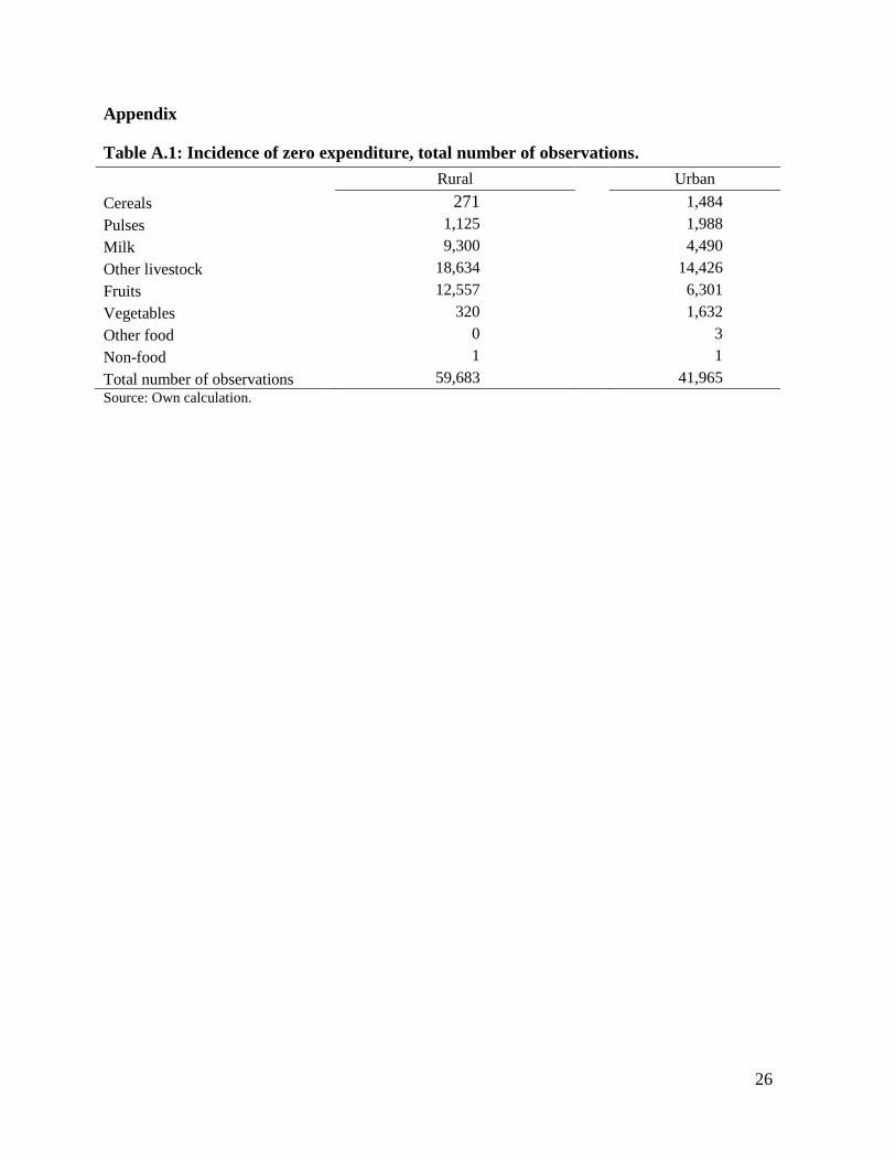
One issue which is common in the use of household expenditure surveys is that of zero

expenditure, as discussed by Deaton (1987) and Ecker and Qaim (2008). There are different

reasons why a household chooses not to consume a commodity. The household either buys the

good at irregular time periods or never buys it altogether, with alcohol and tobacco being the

classic examples (Deaton 1987). Another reason is a too high relative price (corner solution) and

thus the non-consumption of the good is optimal given income and prices. Shonkwiler and Yen

(1999) give a two stage approach to account for zero expenditure through censoring, when zero

consumption is due to a corner solution.3 Nonetheless, we do not account for zero expenditure

due to the following reasons: First, the incidence of zero expenditure is reduced by the

aggregation of food items into composite groups (Tafere et al. 2012). Since the focus of our study

lies on principal food commodities, the level of aggregation is rather high and consequently the

presence of zero expenditure is relatively lower.4 Second, the focus of the Indian diet is

comparatively different, as a large share of the population is vegetarian and the core components

of the Indian food basket are rice, pulses, peas and vegetables (Kumar et al. 2011). These dietary

patterns partly explain zero expenditure for certain food items such as meat.

3 See Shonkweiler and Yen (1999) for further details.

4 The total amount of zero expenditure in each composite group is reported in the Appendix, Table A.1.

8

3.2.3. Unit values and price indices

We calculate a weighted composite group price p𝑗 for each commodity group 𝑖 . We use the

quantities and values of purchased goods, which are reported in the survey, to generate implicit

unit values or prices at the household level, following Wood, Nelson and Nogueira (2012). Unit

values are defined as the ratio of expenditure and quantity and we employ them to calculate

weighted composite group prices as follows. As a first step we calculate weights for each

commodity in the composite group, defined as

𝑎𝑖 =𝑣𝑎𝑙𝑢𝑒 𝑔𝑜𝑜𝑑𝑖

∑ 𝑣𝑎𝑙𝑢𝑒𝑖𝑛𝑖=1

(12)

where good 𝑖 represents one commodity in the composite group and 𝑛 is the number of

commodities in group 𝑖 . We then calculate the composite group price p𝑗 as:

p𝑗 = p𝑖𝑎𝑖 × … × p𝑛

𝑎𝑛 (13)

where 𝑝𝑗 is the composite group price, p𝑖𝑎𝑖 and p𝑛

𝑎𝑛 an are the weighted prices of each commodity

within the group. We then use unit values at the household level to generate median unit values at

the first sampling unit stage. The use of unit values as implicit price is problematic, as discussed

by Deaton (1987), Tafere et al. (2012) and Attanasio et al. (2013). This method has three caveats:

First, unit values at the household level tend to be highly homogeneous. The sampling methods

used for data collection of large household surveys are based on regional clustering.

Consequently, the sampled households have regional proximity to each other. Thus, unit values

are also regionally influenced and lack the variation observed in market prices (Deaton 1987).

Second, unit values can only be considered as approximation to the market price, since unit

values do not account for quality differences among goods, with classic examples being cheap

meat and steak. Quality differences influence the market price and the market price influences

consumers choice (Deaton 1987). Third, measurement errors are likely to affect reported

quantities and expenditure values and are thus passed on to unit values. Moreover, reported

quantities may not be accurate due to imperfect recall (Ecker and Qaim 2008). We are aware of

the issues surrounding the use of unit values as implicit prices; however we proceed with unit

values due to the lack of alternatives.

For non-food items, we use a different approach. Since non-food items are not reported with

quantities, a similar derivation of unit values is not feasible. We follow Robles and Torero (2010)

9

and construct a price index for non-food items for urban and rural regions, based on India’s

Consumer Price Index (CPI). The CPI covers a representative share of non-food commodities

which are also included in the NSS data. In a first step, we construct a sector wise non-food price

index that is a price index for rural and urban areas.5 For standardization, we then employ the all

India non-food price index for industrial workers as reference index. Both CPI series are

published by the Indian Ministry of Statistics and Programme Implementation. The price indices

cover the same time period as the NSS, from July 2011 to June 2012. The standardized, non-food

price index is defined as follows:

𝑃non−food = ∑𝐼𝑖

ℎℎ∈𝑆

𝐼𝑖𝐼𝑛𝑑𝑖𝑎

𝑠ℎ𝑖

𝑖≠𝑓𝑜𝑜𝑑

(14)

where 𝐼𝑖ℎℎ∈𝑆 is a sector wise, non-food consumer price index for rural and urban areas, depending

on the household’s location, 𝐼𝑖𝐼𝑛𝑑𝑖𝑎 is the all India non-food CPI for industrial workers, 𝑠ℎ𝑖 is the

household’s expenditure share on non-food items.

3.3. Empirical Results

3.3.1. Income Elasticities

The estimated parameters of the QUAIDS demand system indicate the fit of the model, and the

majority is significant at the 1 per cent level. Since the parameters are difficult to interpret, we

continue with the calculation of income elasticities. Income elasticities are evaluated at the mean

income. Table 3 shows the estimated income elasticities by region. Income elasticities show the

percentage change in quantity demanded after a one percent change in income. We report the

income elasticities of two estimation trials, in which we estimate the income elasticities for fruits

and vegetables both at the aggregate and at the individual level separately.

When considering the first estimation trail (fruits and vegetables are considered separately), we

find that the income elasticity for commodity groups like cereals, pulses, vegetables and other

food is between zero and one and are thus normal goods. Since their income elasticity is lower

than one, these goods are necessities. Further, we observe the highest income elasticity for fruits,

milk, and non-food items, as well as other livestock products in the rural sector. The income

5 We construct an average index and aggregate over the following non-food items: fuel and lighting, clothing,

bedding, footwear, medical care, education, recreation and amusement, transport and communication, personal care

items, other household requisites, others and miscellaneous.

10

elasticity of these high value goods is greater than one, meaning that these are luxury goods.

Consequently, the percentage change in quantity demanded is higher than the actual income

increase.

When comparing the two estimation trials, we find that the disaggregation of fruits and

vegetables shows that fruits are high value goods. The aggregation of fruits and vegetables

averages out the income elasticities among commodity groups. For both urban and rural regions,

the expenditure elasticity of fruits is greater than one. This means that fruits are luxury goods and

should be considered in the same category as milk, other livestock products and non-food items.

For the remaining commodity groups, we observe comparable income elasticities as in the first

trial.

The estimated income elasticities of some goods are rather high. This is particularly the case for

fruits (1.682), milk (1.692) and other livestock products (1.065) in rural regions. These high

elasticities are due to the quadratic extension of the demand system. Blanks, Blundell and Lewbel

(1997) allow goods to by luxuries at low level of income, while these goods can be normal goods

at high income levels. These results are consistent with the different income levels in rural and

urban regions, with the rural mean income being less than 50 per cent of the average urban

income. Compared to high income elasticities in rural regions, we observe that in urban regions

milk is still luxury goods as per definition. However, the income elasticity of milk is closer to

one, 1.145, as well as the income elasticity for other livestock products is below one, showing the

impact of the higher income level on income elasticities.

The impact of income levels on income elasticities is further corroborated, when analyzing the

results across rural and urban regions. We find the income elasticity to be higher in rural regions.

Due to lower income levels, the expenditure share for food is higher in rural areas, explaining the

higher income elasticities for food items. In urban areas, the income level is higher and thus the

food expenditure share is smaller.

3.3.2. Compensated Own and Cross Price Elasticities

In Table 4 we report compensated own and cross price elasticities, which are evaluated at the

mean value. We start with analyzing own price elasticities, which are defined as the percentage

change of quantity consumed after a one per cent price increase. As expected, our model yields

negative own price elasticities for all commodities. Own price elasticities of the rural sub-sample

11

range between -1.259 and -0.140, while own price elasticities of the urban sector are between

- 1.274 and -0.249. We observe a price elasticity between -1 and 0 for cereals, pulses, vegetables,

other food and non-food. Consequently, their demand is relatively inelastic. The change in

quantity consumed is lower than the percentage change in price. This is consistent with our

results of income elasticities. On the other hand, milk, other livestock, and fruits have an own

price elasticity below -1. Thus, the demand for these goods is relatively elastic, which means that

the change in quantity demanded is larger than the percentage change in price. Consequently, the

consumption of these goods is sensitive to an own price change and a rise in prices leads to a

comparatively strong decline in consumption.

We continue with analyzing cross price elasticities, which are defined as the percentage change

of quantity demanded of one good after a one per cent price increase of another good. A negative

cross price elasticity means that the goods are complements, while a positive cross price elasticity

suggest the goods to be substitutes. If the cross price elasticity is zero, then the goods are

independent and a price increase of one good does not trigger a change in consumption quantities

of the other (Mittal 2010).

The estimated cross price elasticities show that a one percent price increase in cereals triggers a

large consumption response from milk, other livestock products and fruits. Furthermore, in both

sectors we observe negative cross price elasticities for pulses and milk and vice versa, hence

these goods are complementary goods and the consumed quantities decrease in case of a price

increase of the other good. As expected, milk is substituted by other livestock products in case of

a price increase and also vice versa. Regarding fruits, the cross price elasticities are

comparatively moderate. Thus, the consumption of fruits is independent. In the case of a fruit

price increase, the consumption quantities of other livestock, vegetables and cereals increase by

the largest share. In both sectors, a price increase in vegetables triggers a comparatively large

increase in pulses consumption and vice versa.

Our results for income, compensated own and cross price elasticities yield important insights into

consumer behavior. High income and own price elasticities show that these goods are sensitive to

a price increase and the first to be substituted in case of an income decrease or a price increase.

We specifically identify milk, other livestock products and fruits as commodity groups with high

expenditure and own price elasticities. When considering the scenario of a food price increase,

consumers will focus on normal goods, for instance cereals and vegetables, and drop relatively

12

more expensive goods from their consumption basket. Consequently, households consume a less

diversified diet in times of high food prices, focusing their diet on more affordable staple

commodities. High value agricultural commodities play an important role in a diversified and

nutritionally balanced diet, since they are rich in proteins and vitamins. India’s food inflation,

which was led by high value agricultural commodities, therefore threatens to exacerbate the

nutritional status of the Indian consumer.

4. Welfare Analysis

After obtaining compensated own and cross price elasticities, we estimate the welfare impacts of

rising food prices. Our empirical approach comprises first, the estimation of the compensating

variation, and subsequently the impact analysis of a food price increase on India’s poverty ratio.

We follow Deaton (1986) and estimate the compensating variation at the household level. The

compensating variation is the amount needed to compensate a household for a price increase, in

order for the household to remain at the same utility level after a price change. The compensating

variation consists of income and substitution effects.

Following Robles and Torero (2010), the household’s total consumption is defined by the

consumption and production value times the percentage change in food prices:

(𝐪0𝐩1 − 𝐲0𝐩1) − (𝐪0𝐩0 − 𝐲0𝐩0) = (𝐪0 − 𝐲0)∆𝐩 (15)

where 𝐪0, 𝐲0 and 𝐩0 are vector of quantities consumed, quantities produced and prices in the

initial price situation. 𝐩1 is a vector representing the new price level and consequently ∆𝐩

describes the percentage change in prices. Equation 15 describes the case in which households do

not revise their consumption decision.

Furthermore, the household’s net expenditure function, that it the maximum income the

household can achieve, is given by

𝐵(𝐩, 𝐰, 𝑈) = 𝑒(𝐩, 𝐰, 𝑈) − 𝜋(𝐩, 𝐰) (16)

where 𝑒(𝐩, 𝐰, 𝑈) is the total expenditure function and the profit function is described by 𝜋(𝐩, 𝐰).

𝐩 is a price vector of goods, 𝐰 is a vector of factors of production prices and 𝑈 is the utility level.

A second order Taylor approximation around 𝐵(𝐩, 𝐰, 𝑈), that is initial prices and welfare level,

yields the following term for the compensating variation:

13

𝐶𝑉 = 𝑑𝐵(𝐩, 𝐰, 𝑈) = (𝐬ℎ − 𝐬𝑦)′ (

𝑑𝐩

𝐩) 𝑒 +

1

2(

𝑑𝐩

𝐩)

′

(𝒔ℎ)(𝛜𝑖𝑗𝐶 ) (

𝑑𝐩

𝐩) 𝑒 (17)

where 𝑑𝐩/𝐩 is a vector of percentage change of prices, 𝐬ℎ is a vector of expenditure shares of

consumption, 𝐬𝑦 is a vector of expenditure shares of production and 𝑒 is the total household

expenditure.6 𝛜𝑖𝑗

𝐶 is a matrix of compensated own and cross price elasticities, obtained through the

QUAIDS estimation.

The first term (𝐬ℎ − 𝐬𝑦)′(𝑑𝐩/𝐩)𝑒 is the income effect representing the consumer’s loss in

purchasing power after a price increase. When considering only this term, a price increase leads

to a lower budget available for consumption. The second term represents the substitution effect,

which accounts for the substitution of relatively more expensive goods and the reallocation of

budget among food and non-food items. This measure allows us to incorporate first and second

round effects (Robles and Torero 2010). We employ the estimated compensating variation as a

proxy for additional income that a household requires to remain on the same utility level after a

price increase. We subtract the compensating variation from the household’s initial expenditure

level. We then compare the household’s expenditure before and after the food price shock and

analyze the difference between the initial and the new expenditure level (Robles and Torero

2010).

We subsequently analyze the poverty dynamics of a food price shock. The concept of poverty

dynamics refers to the change in national poverty ratios after a rise in food prices. Following

Robles and Keefe (2011), we analyze the percentage share of households that changes the income

group after the price increase. That is the number of households that drops below the poverty

line, due to a rise in food prices. Different to Robles and Torero (2010) we calculate the

household level welfare loss at the poverty line. We then define a new poverty line based on the

additional amount of expenditure required to remain non-poor.

On the basis of the above delineated methodology, we calculate 𝐬ℎ as the ratio of consumption

value of good 𝑖 and total consumption value. Furthermore, we follow Wood, Nelson and

Nogueria (2012) and simulate different food price scenarios, which determine the percentage

change of food prices, 𝑑𝐩/𝐩. India has been experiencing inflationary food prices during the last

five years. Real food prices have increased by 10 per cent (Mishra and Roy 2012). This gives

6 An outright formal derivation of the compensating variation can be found in Robles and Torero (2010), pp.152-155.

14

reason to simulate two food price shocks, to show the effects of a lower and an upper bound

scenario. First, we calculate a food price increase of 10 per cent, as the lower bound, which is

based on the real food price increase. Subsequently, we simulate a 20 per cent food price shock as

upper bound scenario, to understand the effects of persistent and increasing food price inflation.

To measure the impact of different food price scenarios on India’s poverty ratio, we introduce

two income groups in the data set and categorize households accordingly. We follow Kumar et

al. (2011) and base the income groups on India’s official poverty lines, as defined by the

Rangarajan Expert Committee of the Indian Planning Commission. Poverty lines are calculated

on the basis of monthly per capita expenditure during the mixed recall period (30 day recall for

food items, 365 day recall period for non-food goods), as reported in the NSS on household

expenditure (GOI 2014). For the 68th

round of India’s household expenditure survey, the poverty

line7 is defined as Rs. 1407 monthly per capita expenditure in urban areas and Rs. 972 in rural

areas. Hence, we have two income groups, above poverty line and below poverty line, for both

regions. On the basis of these income groups, we compare the household’s expenditure at the

poverty line before and after the price increase and analyze the change in expenditure and the

impact on poverty ratios (Robles and Torero 2010).

A price increase has different effects for food consumers, compared to food producing

households and net food producers. Food consumers are negatively affected, since the rise in

food prices reduces the household budget and the only measure is to substitute relatively

expensive goods for cheaper alternatives. Food producing households are positively affected by

rising food prices, as they sell their goods at a higher price and have the option to consume their

own goods instead of relying on the market. The magnitude of a positive effect depends on the

share of food production in total consumption (De Janvry and Sadoulet 2009). In the present

study, we do not include positive welfare effects for food producing households, since the focus

is on consumers. Furthermore, we require production elasticities to account for production effects

of a food price increase (Robles and Torero 2010). Due to the exclusion of production effects, we

overestimate the welfare effects for food producing households, since we do not account for

income gains arising through high agricultural prices. This is clearly a limitation to our approach.

However, as outlined in the data section of this paper, we find that only 14 per cent of households

7 In 2012, the GOI issued the redefinition of poverty lines, due to claims that the poverty line is set to low. In 2014,

the Rangarajan Expert Committee published new poverty lines, replacing the poverty line of the Tendulkar

committee, which was set at Rs. 816 in rural and Rs. 1000 in urban regions (GOI, 2013).

15

are net food producing households. Still, 86 per cent of food producing households rely to some

extent on the market for their food consumption.

4.1. Compensating Variation

We report the average compensating variation by region (rural and urban) and for mean and

median expenditure in Table 5. When considering the baseline scenario of a 10 per cent food

price increase, we estimate the average loss in rural areas in the range of 5 to 6 per cent of

monthly household income. In money metric terms, a compensation of around Rs. 80 is required

for rural households to remain on the same utility level. For urban areas, we find the

compensating variation to range at 3 to 4 per cent of monthly household expenditure. The money

metric compensation is different for median and mean, with Rs. 23.89 for median and Rs. 93.93

for mean monthly expenditure. The variation across median and mean is quite large, due to the

large expenditure differences within the urban sample. Our results show that households in urban

areas require a larger monetary compensation than rural households. However, rural households

lose a higher percentage share of monthly income and are consequently more negatively affected.

The lower income level in rural areas, as well as the higher expenditure share on food causes the

impact of a food price increase to be higher in rural regions.

In the case of the upper bound scenario of 20 per cent food price increase, we find the welfare

loss to be much larger. Rural households lose 10 to 11 per cent of their monthly income and

require a compensation of Rs. 150 to Rs. 160 to remain on the same utility level. In terms of

percentage share of monthly income, the compensating variation is smaller in urban areas. Urban

households lose 7 per cent of their monthly income and require a mean compensation of Rs.

187.87 per household. Both regions are negatively affected and the magnitude of welfare loss

doubles in coherence with the doubling of food prices.

4.2. Poverty Dynamics

We use our estimates of compensating variation at the household level to analyze the impact of a

food price shock on India’s poverty ratio. As stated above, we use the estimated compensating

variation as an approximation to the post price shock income level and define poverty dynamics

as the share of households that drops below the poverty line after a food price increase. The

estimates for poverty dynamics in rural and urban regions and for the two income groups are

reported in Table 6.

16

In the baseline scenario of a 10 per cent food price increase, we find that an additional 4.69 per

cent of rural households become poor. In the initial setting, 37.7 per cent of rural households have

a monthly income below the poverty line. Hence, the total share of poor households in rural areas

increases to 42.39 per cent. In urban areas, the change in poverty rates is of smaller magnitude.

Yet we find that 2.19 per cent of households, which were above the poverty line before the food

price increase, are poor after the price shock. Compared to the initial level of 26 per cent of urban

households below the poverty line, 28.19 per cent of urban households now have an income

below the poverty line.

For the case of a 20 per cent food price increase, the impact on India’s poverty ratio is larger. Our

results suggest that an additional 9.32 per cent of rural households drop below the poverty line

after a 20 per cent food price increase. The total share of poor households in rural areas increases

from 37.7 to 47.02 per cent. As in the 10 per cent scenario, the impact on urban households is less

pronounced. We find that further 4.52 per cent of urban households fall below the poverty line.

Consequently, the overall share of poor households increases from 26 to 30.52 per cent in urban

areas.

Apart from the households where we observe the impact of high food prices due to their poverty

entry from above the poverty line to below the poverty line, we stress that our model shows an all

losing scenario. That means that the net income level of all households decreases. Households

below poverty line become poorer, as well as households above poverty line have a lower

income. The magnitude of the impact depends largely on how much the households spends on

food, in relation to their overall income level.

Our results indicate that rural households are more negatively affected by a food price increase

than urban households, with an average loss of around 5 per cent of monthly income.

Importantly, we have not included positive impacts of rising prices for food producing

households, hence our estimates should be considered as upper bound for food producing

households. Our results are consistent with previous studies by de Janvry and Sadoulet (2009),

who also find that rural households have the highest welfare loss in the case of a food price

increase. These findings suggest that policy responses to high food prices should particularly

target rural households.

17

Moreover, we show that India’s food inflation of 10 per cent drives additional 4.69 per cent of

rural and 2.19 per cent of urban households into poverty. The scenario of a 10 per cent price

increase describes what consumers faced during the period of food price inflation.

5. Conclusion

In this paper we explore how inflationary food prices impact India’s consumer welfare and

poverty ratios. We account for changes in consumption patterns, i.e. substitution effects among

food items, by including own and cross price elasticities obtained through the estimation of a

demand system, i.e. QUAIDS.

The estimation of QUAIDS and the respective results for income, compensated own and cross

price elasticities show that high value food commodities, for instance milk, other livestock

products and fruits, are the most sensitive to an own price change, as well as to a change in

income. In times of increasing food prices, consumers substitute high value food items for

cheaper alternatives. Consequently, households consume a less diversified diet in times of high

food prices, focusing their diet on cheaper staple commodities. High value agricultural goods

play an important role in a diversified and nutritionally balanced diet, since they are rich in

proteins and vitamins. India’s food inflation, which has been led by high value agricultural

commodities, therefore threatens to exacerbate the nutritional status of the Indian consumer.

India’s TPDS, as well as the newly introduced NFSA are based on cereals and the access to food,

rather than nutrition security. Particularly poor households substitute expensive food items by

cheaper alternatives and hence switch to a cereals lead diet. This causes nutritional deficiencies

and should be addressed by the already implemented food distribution scheme. The scope of food

security programs needs to be extended to nutrition security.

The results of our welfare analysis suggest that rural households suffer a larger welfare loss than

urban households. The simulation of a 10 per cent food price increase indicates that rural

households lose 5 to 6 per cent of their monthly income, while urban households lose 3 to 4 per

cent. The impact analysis of a food price increase on India’s poverty ratio shows that additional

4.69 per cent of households in rural areas and 2.19 per cent of households in urban areas are

driven into poverty. This scenario, which is based on India’s real food price inflation, represents a

large throwback in India’s fight against poverty and hunger. As upper bound scenario, we show

that a 20 per cent food price increase would further cause additional 9.32 per cent of rural and

18

4.52 per cent of urban households to fall below the poverty line. We conclude that India’s current

food inflation has a strong negative impact on India’s poverty ratio.

19

Tables and Figures

Table 1: Sample characteristics of the Indian household expenditure survey.

Rural Urban all India

Sex of household head (male, %) 88 88 88

Mean age of household head 46 44 45

Education of household head (%) Not literate 39.07 15.35 31.66

Literate without formal schooling 0.6 0.4 0.5

Literate with formal schooling (below primary - secondary) 51.3 49.8 50.8

Higher secondary and diploma / certificate course 5.36 13.8 8.00

Graduate 2.86 14.1 6.37

Postgraduate 0.8 6.5 2.58

Mean household size 4.6 4.05 4.43

Mean number of adults 2.88 2.78 2.85

Mean number of children 1.31 0.97 1.21

Mean monthly per capita expenditure (Rs.)1 1375.28 2817.69 1826.99

Income groups2 (%)

Below the poverty line 37.7 26.0 34.1

Above the poverty line 62.3 74.0 65.9

Food expenditure share (%) 52.7 43.1 49.7

Total food producers 36,501 6,147 42,648

Mean home food production value (Rs.) 993.54 699.74 973.53

Number of observations 59,683 41,965 101,648 11 Rs.= 0.02 US$ (average exchange rate during the sample period from July 2011 to June 2012; data: Federal

Reserve Bank of St. Louis). 2 Poverty lines as defined in GOI, 2014.

Source: Own calculation.

20

Table 2: Composite commodity groups.

Group Name Items 1 Cereals Rice PDS, rice other sources, flattened rice (chira), popped rice (khoi,

lawa), puffed rice (muri), other rice products, wheat PDS, wheat other

sources, finely milled wheat flour (maida), finely milled wheat (suji,

rawa), noodles, bread, other wheat products, Sorghum (jowar), pearl

millet (bajra), barley, small millets, finger millet (ragi), maize and their

respective products, other cereals.

2 Pulses Pigeon peas (Arhar, tur), peas, split and whole (gram), moong bean

(moong), lentils (masur), black split pea (urd), peas, grass pea

(khesari), other pulses, pea products, pulse flour (besan), other pulses

products. 3 Milk Liquid milk, baby food, condensed and powder milk, curd, ghee,

butter.* 4 Other livestock Eggs, fish, prawn, goat meat, beef and buffalo meat, pork, chicken,

others (birds, crab, oyster, tortoise).

5 Fruits Fresh fruits: banana, jackfruit, water melon , guava, singara, papaya,

mango, cantaloupe melon (kharbooza), pears (nashpati), berries, litchi,

apple, grapes, other fresh fruits; dry fruits: coconut (copra), groundnut,

dates, cashew nut, walnut, other nuts, raisin, dry grapes (kishmish),

other dry fruits.* 6 Vegetables Potatoes, onion, tomato, eggplant (brinjal), radish, carrot, spinach

(palak) and other leafy vegetable, green chilis, okra (lady's fingers),

snake gourd (parwal), cauliflower, cabbage, gourds, pumpkin, peas,

beans, long beans (barbati), lemon, other vegetables. 7 Other food Goods belonging to the categories salt and sugar, edible oil, spices,

beverages, served and packaged processed food, betal leaves, tobacco,

intoxicants.*

8 Non food All remaining goods and services, as indicated in the NSS schedule.

Note: * A number of food items are not reported with consumption quantities (or in non-kg consumption quantities)

and are thus not eligible for the derivation of unit values. The following goods were excluded from the group

aggregates (names and numbers as in the NSS schedule): Milk: ice cream (166), other milk products (167),

Fruits: pineapple (223), coconut (224), green coconut (225), oranges (228), other fresh fruits (238); Other

food: other beverages (277), cooked snacks purchased (283), other served processed food (284), prepared

sweets (290), biscuits and chocolates (291), other packaged processed food (296), ingredients for mouth

refresher (pan) (302), other tobacco products (317), and other intoxicants (325).

Source: National Sample Survey Office (2013a).

21

Table 3: Income elasticities.

1st Estimation 2nd Estimation

Rural Urban Rural Urban

Cereals 0.256 0.158 0.285 0.185

Pulses 0.392 0.278 0.369 0.243

Milk 1.692 1.145 1.664 1.123

Other livestock 1.065 0.824 1.073 0.822

Fruits 1.682 1.628

Vegetables 0.313 0.295

Fruits and vegetables

0.619 0.654

Other food 0.652 0.565 0.652 0.559

Non food 1.259 1.242 1.257 1.249

Note: In the first estimation, we estimate the expenditure shares of fruits and vegetables separately. In the second

estimation fruits and vegetables are aggregated into one composite commodity group.

Source: Own calculation.

Table 4: Compensated own and cross price elasticities.

Rural

Change in

quantity: Cereals Pulses Milk

Other

livestock Fruits Vegetables

Other

food

Non

food

Cereals -0.140 -0.005 0.116 0.095 0.027 0.003 0.042 -0.137

Pulses -0.021 -0.592 -0.098 0.131 0.006 0.262 0.013 0.299

Milk 0.198 -0.041 -1.053 0.270 -0.001 0.092 0.035 0.500

Other livestock 0.275 0.097 0.478 -1.259 0.044 0.054 0.358 -0.047

Fruits 0.249 0.014 -0.004 0.138 -1.121 0.108 0.122 0.494

Vegetables 0.007 0.162 0.132 0.046 0.028 -0.690 0.059 0.257

Other food 0.039 0.003 0.018 0.111 0.012 0.022 -0.685 0.480

Non-food -0.037 0.020 0.082 -0.005 0.014 0.028 0.142 -0.244

Urban

Change in

quantity: Cereals Pulses Milk

Other

livestock Fruits Vegetables

Other

food

Non

food

Cereals -0.298 0.002 0.196 0.035 0.027 0.024 0.030 -0.017

Pulses 0.008 -0.548 -0.101 0.103 0.002 0.220 -0.004 0.320

Milk 0.264 -0.036 -1.031 0.279 -0.002 0.106 -0.038 0.458

Other livestock 0.087 0.071 0.540 -1.274 0.061 0.068 0.247 0.200

Fruits 0.164 0.003 -0.008 0.140 -1.091 0.082 0.116 0.594

Vegetables 0.055 0.135 0.177 0.060 0.030 -0.559 0.008 0.094

Other food 0.021 -0.001 -0.022 0.071 0.014 0.002 -0.649 0.562

Non-food -0.003 0.016 0.062 0.013 0.018 0.008 0.136 -0.249

Note: Own price elasticities on the diagonal, cross price elasticities off the diagonal.

Source: Own calculation.

22

Table 5: Compensating variation, 10 and 20 per cent food price increase.

10 % scenario

Rural

Urban

Compensating variation: Median Mean

Median Mean

% of monthly income 5.97 5.18

3.63 3.61

in Rs. 77.03 83.17

23.89 93.93

20 % scenario

Rural

Urban

Compensating variation: Median Mean

Median Mean

% of monthly income 11.94 10.36

7.26 7.22

in Rs. 154.07 166.33

47.78 187.87

Note. Includes only net consuming households.

Source: Own calculation.

Table 6: Poverty dynamics, 10 and 20 per cent food price increase.

Initial Scenario

10 % Scenario

20 % Scenario

Dynamic Rural Urban Rural Urban Rural Urban

BPL 37.7 26.0

42.39 28.19

47.02 30.52

APL 62.3 74.0

57.61 71.81

52.98 69.48

Change in poverty 4.69 2.19 9.32 4.52

Note: Estimates are based on monthly income at the poverty line.

Source: Own calculation.

Figure 1: Indian wholesale price index of various food items, 2005-2014.

Source: Indian Ministry of Commerce and Industry.

0.0

50.0

100.0

150.0

200.0

250.0

300.0

350.0

400.0

450.0

01/2

00

5

05/2

00

5

09/2

00

5

01/2

00

6

05/2

00

6

09/2

00

6

01/2

00

7

05/2

00

7

09/2

00

7

01/2

00

8

05/2

00

8

09/2

00

8

01/2

00

9

05/2

00

9

09/2

00

9

01/2

01

0

05/2

01

0

09/2

01

0

01/2

01

1

05/2

01

1

09/2

01

1

01/2

01

2

05/2

01

2

09/2

01

2

01/2

01

3

05/2

01

3

09/2

01

3

01/2

01

4

05/2

01

4

09/2

01

4

Cereals Pulses Vegetables Fruits Milk Eggs, Meat and Fish

23

Acknowledgments

I thank Devesh Roy, Akanksha Negi, Miguel Robles, Suman Chakrabati and Marta Kozicka

for their many useful comments. Financial support was granted by the Advisory Service on

Agricultural Research for Development of GIZ and the International Food Policy Research

Institute (IFPRI).

References

Attanasio, O. et al., 2013. Welfare Consequences of Food Price Increases: Evidence from Rural

Mexico. Journal of Development Economics 104, 136-151.

Blanks, J., Blundell, R., Lewbel, A., 1997. Quadratic Engel Curves and Consumer Demand. The

Review of Economics and Statistics, Vol. 79, No.4, 527-539.

De Janvry, A., Sadoulet, E., 2009. The Impact of Rising Food Prices on Household Welfare in India.

Working Paper Series Institute for Research on Labor and Employment, University of

California at Berkeley.

Deaton, A., 1986. Demand Analysis, Handbook of Econometrics, in Z. Griliches, M. D. Intriligator,

eds., Handbook of Econometrics, Volume 3, Chapter 30, 1767-1839, Elsevier.

,1987. Estimation of Own- and Cross-Price Elasticities from Household Survey Data. Journal

of Econometrics 36, 7-30.

Deaton, A., Muellbauer, J., 1980. An Almost Ideal Demand System. The American Economic Review,

Vol. 70, No. 3, 312-326.

Ecker, O., Qaim, M., 2008. Income and Price Elasticities of Food Demand and Nutrient Consumption

in Malawi. 2008 Annual Meeting at the American Agricultural Economics Association, July

27-29, Orlando, Florida.

Ganguli, K., Gulati, A., 2013. The Political Economy of Food Price Policy: The Case Study of India.

WIDER Working Paper No. 2013/034, United Nations University.

GOI, 2013. Press Note on Poverty Estimates, 2011-2012. Planning Commission, New Delhi, available

at http://planningcommission.nic.in/news/pre_pov2307.pdf, last accessed on 16.04.2014.

GOI, 2014. Report of the Expert Group to Review the Methodology for Measurement of Poverty.

Planning Commission, New Delhi, available at

http://planningcommission.nic.in/reports/genrep/pov_rep0707.pdf, last accessed on

11.06.2015.

24

Gulati, A., Gujra, J., Nandakumar, T. et al., 2012. National Food Security Bill - Challenges and

Options. Discussion Paper No. 2, Commission for Agricultural Costs and Prices, New Delhi.

Gulati, A., Saini, S., 2014. Food Inflation in India: Diagnosis and Remedies, in U. Kapila, eds., Indian

Economy Since Independence, 15th Edition. New Delhi: Academic Foundation.

Jehle, G. A., Reny, P. J. (2011): Advanced Microeconomic Theory, Financial Times, Prentice Hall.

Jha, S., Srinivasan, P. V., 2004. Achieving Food Security in a Cost Effective Way: Implications of

Domestic Deregulation and Reform under Liberalized Trade. MTID Discussion Paper No.

67, IFPRI.

Kotwal, A., Ramaswami B., Murugkar M., 2011. PDS Forever? Economic and Political Weekly, Vol.

XLVI, No. 21, 72-76.

Kozicka, M. et al., 2015. Modelling Indian Wheat and Rice Sector Policies. ZEF Discussion Paper on

Development Policy No. 197.

Kumar, P. et al., 2011. Estimation of Demand Elasticity for Food Commodities in India. Agricultural

Economics Research Review, Vol. 24 January-June 2011, 1-14.

Menon, P., 2013. Tackling Malnutrition in India. IFPRI Blog, available at

http://www.ifpri.org/blog/tackling-malnutrition-india, last accessed on 14.04.2014.

Mittal, S., 2010. Application of the QUAIDS Model to the Food Sector in India. Journal of

Quantitative Economics, Vol. 8, No 1, 42-54.

Mishra, P., Roy, D., 2012. Explaining Food Inflation in India: The Role of Food Prices, in S. Shah, B.

Bosworth, A. Panagariya, eds., India Policy Forum 2011/12, Volume 8, National Council of

Applied Economic Research and Brookings Institution.

Mishra, P., 2013. Financial and Distributional Implications of the Food Security Law. Economic and

Political Weekly, Vol. XLVIII, No. 39, 28-30.

Muellbauer, J., 1976. Community Preference and the Representative Consumer. Econometrica, Vol.

44, No. 5.

National Sample Survey Office, 2013a. 68th Round of Household Expenditure Survey. Planning

Commission, New Delhi.

, 2013b. Note on Sample Design and Estimation Procedure of the NSS 68th Round. Ministry

of Statistics and Program Implementation, New Delhi.

25

Poi, B. P., 2012. Easy Demand-System Estimation with Quaids. The Stata Journal 12, Number 3, 433-

446.

Robles, M., Torero, M., 2010. Understanding the Impact of High Food Prices in Latin America.

Economia, 117-159.

Robles, M., Keefe, M., 2011. The Effects of Changing Food Prices on Welfare and Poverty in

Guatemala. Development in Practice, 21:4-5, 578-589.

Saini, S., Kozicka, M., 2014. Evolution and Critique of Buffer Stocking Policy of India, ICRIER

Working Paper No. 283.

Shonkwiler, J. S., Yen, S. T., 1999. Two-Step Estimation of a Censored System of Equations.

American Journal of Agricultural Economics, Vol. 81, No. 4, 972-982.

Tafere, K. et al., 2012. Food Demand Elasticities in Ethiopia: Estimates Using Household Income

Consumption Expenditure Survey Data. IFPRI, Ethiopia Strategy Support Program II,

Working Paper 11.

Wood, B. D. K., Nelson, C., Nogueira, L., 2012. Poverty Effects of Food Price Escalation: The

Importance of Substitution Effects in Mexican Households. Food Policy 37, 77-85.

World Bank, 2014. Prevalence of Undernourishment as Percentage Share of Population. Available at

http://data.worldbank.org/indicator/SN.ITK.DEFC.ZS, last accessed on 15.04.2014.

26

Appendix

Table A.1: Incidence of zero expenditure, total number of observations.

Rural

Urban

Cereals 271

1,484

Pulses 1,125

1,988

Milk 9,300

4,490

Other livestock 18,634

14,426

Fruits 12,557

6,301

Vegetables 320

1,632

Other food 0

3

Non-food 1

1

Total number of observations 59,683

41,965 Source: Own calculation.