well log analysis at the white rose oilfield, offshore ... log analysis of white rose field crewes...

Well log analysis of White Rose field

CREWES Research Report — Volume 17 (2005) 1

Well log analysis at the White Rose oilfield, offshore Newfoundland

Jessica Jaramillo Sarasty and Robert R. Stewart

ABSTRACT The petrophysical analysis in this paper is based on dipole sonic (Vp and Vs), density,

gamma-ray, and porosity (density porosity and neutron porosity) logs from wells in the White Rose oilfield, offshore Newfoundland. In general, Vp and Vs increase with depth, Vp/Vs decreases with depth, velocity increases as total porosity decreases, Vp/Vs decreases slightly when total porosity decreases, and Vs shows a high correlation with porosity.

We also applied empirical Castagna’s (1985), Faust’s (1951), Gardner et al.’s (1974) and Pickett’s (1963) relationships. We find that Faust is the better predictor for Vp, Castagna is a better predictor for Vs, Castagna’s limestone relationship works better than Pickett’s limestone relationship, and the Gardner prediction of ρ should be used with caution.

Empirical relationships apply with a variable levels of accuracy. Better fits can be achieved by dividing the lithologies into formations (Jaramillo and Stewart, 2003).

INTRODUCTION The White Rose field is located on the northeastern edge of the Jeanne d'Arc Basin,

approximately 350 km southeast of St. John's, Newfoundland (Figure 1). The White Rose field is 50 km from both the Hibernia and Terra Nova oilfields. The water depth is about 120 m. The target reservoir is the Aptian Avalon sandstone.

FIG. 1. Location of White Rose oilfield, Newfoundland (Modified from Encarta.msn.com, 2004.).

Jaramillo Sarasty and Stewart

2 CREWES Research Report — Volume 17 (2005)

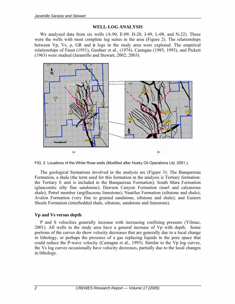
WELL-LOG ANALYSIS We analyzed data from six wells (A-90, E-09, H-20, J-49, L-08, and N-22). These

were the wells with most complete log suites in the area (Figure 2). The relationships between Vp, Vs, ρ, GR and φ logs in the study area were explored. The empirical relationships of Faust (1951), Gardner et al., (1974), Castagna (1985; 1993), and Pickett (1963) were studied (Jaramillo and Stewart, 2002; 2003).

FIG. 2. Locations of the White Rose wells (Modified after Husky Oil Operations Ltd, 2001.).

The geological formations involved in the analysis are (Figure 3): The Banquereau Formation, a shale (the term used for this formation in the analysis is Tertiary formation: the Tertiary E unit is included in the Banquereau Formation); South Mara Formation (glauconitic silty fine sandstone); Dawson Canyon Formation (marl and calcareous shale); Petrel member (argillaceous limestone); Nautilus Formation (siltstone and shale); Avalon Formation (very fine to grained sandstone, siltstone and shale); and Eastern Shoals Formation (interbedded shale, siltstone, sandstone and limestone).

Vp and Vs versus depth P and S velocities generally increase with increasing confining pressure (Yilmaz,

2001). All wells in the study area have a general increase of Vp with depth. Some portions of the curves do show velocity decreases that are generally due to a local change in lithology, or perhaps the presence of a gas replacing liquids in the pore space that could reduce the P-wave velocity (Castagna et al., 1993). Similar to the Vp log curves, the Vs log curves occasionally have velocity decreases, partially due to the local changes in lithology.



Vp/Vs versus depth This analysis was conducted on wells H-20 and L-08. A decrease of Vp/Vs with depth

is observed. Shallow values are in the 2.5–3.5 range. Deeper values are closer to ~1.6. Within lithological formations we observe some increase of the Vp/Vs values. The increase of pressure and temperature could generate bulk porosity reductions, phase changes, cementation, and additional diagenetic changes that could result in compressional and shear velocity gradients (Castagna et al., 1993).

FIG. 3. Stratigraphy of the White Rose field (From Deutsch/Meehan-Husky Oil, 2000, in Husky Oil Operations Ltd, 2001.).

Velocity from Faust’s relationship Faust’s empirical relationship can be written as

)( 61

ZTCV pp = (1)

where Vp is the compressional velocity (m/s), Cp is 125.3 (constant), T is formation age (millions of years) and Z is depth of burial (m). Equation 1 predicts compressional velocities as a function of geological time and depth of burial of the rock (Faust, 1951). This section compares the predicted Vp from the Faust relationship with measured or actual Vp values.



The results obtained using Faust’s equation gave only approximate estimates for the Tertiary formations, and significant underestimated for the Cretaceous formations (Figure 4 and Table 1). It was necessary to segment the wells into their main formations and try to evaluate the best-fit Vp curve using Faust’s equation

In Figure 4, the curve using the Faust constant (Cp=125.3) is labelled “curve A” and the curve with the derived constant (derived from a least square fit) is labelled “curve B”. Each predicted curve is compared with the actual Vp log curve (Panels (b) and (c)).

After comparing both RMS error values (Figure 4, Table 1), we can conclude that original Cp curve data constant (Cp=125.3) works best for the younger Tertiary formations. The derived constant, Cp=132.38, works better for the Cretaceous formations. Tertiary sediments are mostly clastics. In the Cretaceous formations, there is limestone present. In general, the results obtained from the Faust equation must be regarded with caution since the Faust equation was formulated using clastic data.

FIG. 4. Data from well H-20: Panel (a) — actual Vp and Faust Vp (curves A and B) versus depth. Panel (b) — percentage error between the actual Vp curve and the Faust Vp curve A (derived using 125.3 as the constant): RMS error is ±398.01 m/s; Panel (c) — percentage error between the actual Vp curve and the Faust Vp curve B (derived using 128.90 as the constant): RMS error is ±387.45 m/s.



Table 1. Constants used to predict Vp from Faust’s relationship for all wells. The RMS from using Faust’s constant and the RMS error from using the derived constant gives the accuracy of the derived constant. The derived constant is per well.

Well Faust Constant RMS error± (m/s) Constants derived RMS error± (m/s)

A-90 125.3 1344.12 132.38 846.06

E-09 125.3 546.16 127.53 542.83

H-20 125.3 398.01 128.90 387.45

J-49 125.3 445.15 126.06 444.64

L-08 125.3 381.07 120.50 360.54

N-22 125.3 389.89 123.74 387.31

Actual Vs versus Vs estimated from Faust’s relationship We explored the possibility of predicting Vs using a relationship similar to the one

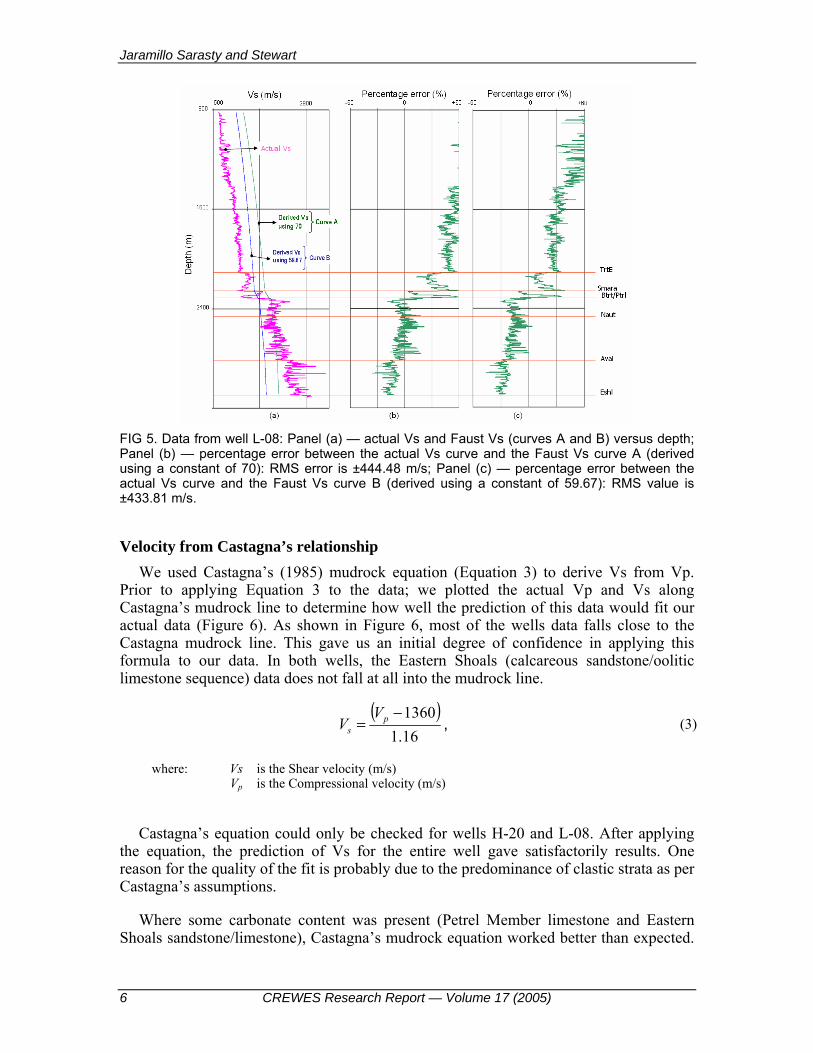
used to predict Vp from Faust (1951), Equation 2. The “Vs Faust equation” attempts to predict shear velocities as a function of geological time and depth of burial of the rock. We explored this relationship in wells H-20 and L-08 where the shear velocity was acquired (Figure 5). The predictions are not very accurate. The constants for each well (Table 2) were derived from the log Vs curve and from the Faust relationship

)( 61

ZTCV ss = (2)

where Vs is the shear velocity (m/s), Cs is 70 (constant), T is formation age (millions of years) and Z is depth of burial (m).

The results obtained using Faust equation and the derived constant gave a better Vs curve for the Tertiary formations. However, the results from both the Tertiary and Cretaceous formations are, at best, approximate (Figure 5 and Table 2). The quality of these results (Figure 5) could also be due to the observation that the sequence is mainly clastic but still contains limestones that can affect the determination of the constant. The best results were found in well H-20. Well L-08 had a fair result for the Tertiary formations.

Table 2: Constants used to predict Vs from Faust’s relationship for wells H-20 and L-08. The RMS error from using Faust’s constant and the RMS error from using the derived constant show the accuracy of the derived constant. The derived constant is per well.

Well Faust Constant RMS error ± (m/s) Constants derived RMS error ± (m/s)

H-20 70 444.48 65.53 429.80

L-08 70 508.53 59.67 433.81



FIG 5. Data from well L-08: Panel (a) — actual Vs and Faust Vs (curves A and B) versus depth; Panel (b) — percentage error between the actual Vs curve and the Faust Vs curve A (derived using a constant of 70): RMS error is ±444.48 m/s; Panel (c) — percentage error between the actual Vs curve and the Faust Vs curve B (derived using a constant of 59.67): RMS value is ±433.81 m/s.

Velocity from Castagna’s relationship We used Castagna’s (1985) mudrock equation (Equation 3) to derive Vs from Vp.

Prior to applying Equation 3 to the data; we plotted the actual Vp and Vs along Castagna’s mudrock line to determine how well the prediction of this data would fit our actual data (Figure 6). As shown in Figure 6, most of the wells data falls close to the Castagna mudrock line. This gave us an initial degree of confidence in applying this formula to our data. In both wells, the Eastern Shoals (calcareous sandstone/oolitic limestone sequence) data does not fall at all into the mudrock line.

( )

16.11360−

= ps

VV , (3)

where: Vs is the Shear velocity (m/s) Vp is the Compressional velocity (m/s)

Castagna’s equation could only be checked for wells H-20 and L-08. After applying the equation, the prediction of Vs for the entire well gave satisfactorily results. One reason for the quality of the fit is probably due to the predominance of clastic strata as per Castagna’s assumptions.

Where some carbonate content was present (Petrel Member limestone and Eastern Shoals sandstone/limestone), Castagna’s mudrock equation worked better than expected.



A simpler approach to Vs prediction for carbonate lithology, is to use Pickett’s empirical relationship for limestones (1963). Pickett’s equation is shown as Equation 4.

9.1p

s

VV = , (4)


Equation 4 was empirically derived using laboratory core data to predict Vs for carbonates. Castagna (1993) based his carbonate equation on a quadratic form (an extension of Pickett’s equation) and a least-squared polynomial fit to the data (Equation 5):

0305.10168.105509.0 2 −+−= pps VVV , (5)


This limestone empirical relationship gives better results for the limestone section of our well than when using the mudrock equation.

The quadratic expression (Equation 5) for limestone uses three constants plus Vp to predict shear velocities. The Vs results are satisfactory on well L-08 (Figure 7), the results are more encouraging for the Petrel member. In the same well, the resultant Vs values from Castagna’s mudrock equation for clastics are higher than the actual Vs values. The results for the Eastern Shoals Formation are reasonable. The Castagna-derived Vs for limestones is more realistic than the Castagna Vs for clastics.

The data shown in Figure 7 are from well L-08. Row (1) column (a) shows actual Vs and Castagna Vs (derived from Castagna’s mudrock relationship) versus depth. Row (1) column (b) shows actual Vs and Castagna Vs (derived from Castagna’s limestone relationship) versus depth. Row (1) column (c) shows actual Vs and Castagna Vs (derived from Pickett’s relationship) versus depth.

Row (2) column (a) is a closer look at the Petrel Formation, actual Vs and Castagna Vs (derived from Castagna’s mudrock relationship) versus depth. Row (2) column (b) is a closer look at the Petrel Formation, actual Vs and Castagna Vs (derived from Castagna’s limestone relationship) versus depth. Row (2) column (c) is a closer look to the Petrel Formation, actual Vs and Castagna Vs (derived from Pickett’s relationship) versus depth.

Row (3) column (a) is a closer look at the Eastern Shoals Formation, actual Vs and Castagna Vs (derived from Castagna’s mudrock relationship) versus depth. Row (3) column (b) is a closer look at the Eastern Shoals Formation, actual Vs and Castagna Vs (derived from Castagna’s limestone relationship) versus depth. Row (3) column (c) provides a closer look at the Eastern Shoals Formation, actual Vs and Castagna Vs (derived from Pickett’s relationship) versus depth.



FIG 6. Panel (a) — actual Vs versus actual Vp for well H-20. The data falls close to the original Castagna’s mudrock line. Panel (b) — actual Vs versus actual Vp for well L-08. Again cluster near the mudrock line.

Table 3, shows the RMS values for the entire well L-08, and also the carbonate Formations present in the well (Petrel and Eastern Shoals). The best result for the entire well uses the mudrock equation. For the Petrel Formation and the Eastern Shoals Formation, the limestone relationship gives a better result than Pickett’s relationship.



FIG 7. Data from well L-08. Actual and derived Vs (using Mudrock, limestone and Pickett’s relationships) versus depth.



Table 3. RMS analysis for the different Vs curves obtained in well L-08. The RMS values accord to the relationship used to derive Vs. Key: indicates good RMS results

RMS error± (m/s)

Vs derived from Thickness (m)

Mudrock relationship

Castagna’s limestone relationship

Pickett’s relationship

All Formations 2293.25 107.31 175.83 305.48

Petrel 148.88 152.48 51.89 165.86

Eastern Shoals 21 509.05 162.75 688.58

Velocity versus GR The gamma ray results on the wells show a common trend for the corresponding

lithology. As we go from shales and limestones into sandstones, the velocities increase.

In Figure 8, one can observe a general trend on both wells in the Vp/Vs versus GR relationship: Vp/Vs increases with increasing GR values. High Vp/Vs values (3.5–4.0) are related to the Tertiary formation (shallow rocks), which correlate with high GR values (60–130, Banquereau shales). As the depth increases, the GR values decrease (going from shales into carbonates and sandstones) and Vp/Vs decreases. Probably mostly due to lithology, age, and compaction/pressure.

If we compare the Nautilus and Avalon GR and Vp/Vs values, we notice that the GR values for the Nautilus shales have a range of 8–129 and for the Avalon Formation 6–137. Their Vp/Vs values are also similar to each other (1.54–2.07 versus 1.42–2.03). These different ranges overlay each other (Figure 8a) and therefore could make it difficult to distinguish between the two lithologies based exclusively on Vp/Vs and GR.

Gardner density In using Gardner’s equation (Equation 6), density can be derived from Vp and

Gardner’s constants, a and m. Gardner et al. (1974) give values for a and m of 310 and 0.25, respectively. This section compares the predicted ρ from Gardner’s equation with actual ρ values.

maαρ = , (6)

where: ρ Density (kg/m3) a Constant of 310

α Compressional velocity (m/s) m Constant of 0.25 For wells E-09 and well H-20 (Figure 9, Panel a), where the ρ prediction was done for

the section of the well where ρ was acquired, Gardner’s rule does a better job in predicting the ρ in comparison to the other wells. Wells J-49, L-08 (Figure 9, Panel (b)), and N-22, Gardner’s equation had difficulties predicting ρ using 310 as constant. There is significant scatter in the data.



To derive a new and more suitable constant per well, we derived the constant from the actual density value and Gardner et al.’s empirical equation. With these new constants we were able to fit the data (Table 2.13). Also, with the help of the RMS error values we were able to corroborate where the relationship worked better.

The RMS error values (Table 4) show that the best results use the derived constant. For well H-20 (Figure 9, Panel (a)), using both Gardner’s constant and the derived constant give similar results and RMS error values of ±58.79 m/s.

FIG 8. Panel (a) — Vp/Vs versus GR for well H-20. Panel (b) — Vp/Vs versus GR for well L-08. Note that the Tertiary Formation keeps a siltstone range of values as the well goes deeper. The differentiation of Formations is noticeable. In both wells, the relationships behave quite similarly: as Vp/Vs decreases, GR decreases.

As shown for well L-08 in Figure 9, Panel (b), Gardner et al.’s rule has difficulty predicting ρ. There are three clusters in the data. However, the RMS error values (Table 4) are considered reasonable.



According to Castagna et al. (1993), the use of Gardner’s equation has a tendency to overvalue the density for sandstones and undervalue the density for shales. Our results show a different trend. The shales tend to have an underestimation in the density values like Castagna’s, but the density of the sandstones does not follow a general trend. From the five wells that were analyzed (E-09, H-20, J-49, L08, and N-22), six formations were treated as sandstones (South Mara, Dawson Canyon, Avalon, Eastern Shoals, Hibernia, Lower Hibernia, and Jeanne d’Arc). It is important to remember that these formations are not an absolute package of sandstones; we can find shales, limestones, and siltstones within these formations. This variation in lithology within the “sandstone formations” should explain why the final density results do not show a general trend (the values are undervalued and overvalued for this group of rocks). The final Castagna’s results came from the Gulf of Mexico and not Eastern Canada. This may be a reason why the results were only fair. The presence of carbonates could also mislead the predicted values.

The results should be taken with sufficient caution, keeping in mind the different lithologies that are involved in the analysis.

Table 4. Constants used to predict ρ from Vp using Gardner’s relationship for all wells. The RMS from using Gardner’s constant and the RMS error from using the derived constant give the accuracy of the derived constant. The derived constant is per well. Key: indicates good RMS results

Well Gardner Constant RMS error± (m/s) Constants derived RMS error ± (m/s)

E-09 310 144.61 320.24 118.64

H-20 310 58.79 310.14 58.79

J-49 310 247.06 314.80 244.21

L-08 310 112.25 319.31 88.65

N-22 310 124.41 318.76 104.61

Density from Vs We evaluated the prediction of ρ using Vs. This new approach (Equation 7) is based

on Gardner et al.’s equation (1974), (Equation 6). This section compares the predicted ρ from Equation 7 with the actual ρ value. We performed this comparison for all the data on well L-08 and for the data from the bottom section of well H-20 (2272–3271 m).

msaV=ρ , (7)

where: ρ Density (kg/m3) a Constant of 350 or derived constant

Vs Shear velocity (m/s) m Constant of 0.25 As Vs < Vp, we expected the new constants to be higher. Deriving the constant, we

found that well H-20 has a 352.73 constant, and well L-08 uses a 386.02 constant (Table 5) and Figure 10. The exponent m = 0.25 was used. The results for the entire wells were not overly accurate (Figure 10).



Velocity and density properties depend on different factors, including type of rock, porosity, mineral composition, and fluid properties. These factors in turn are affected by overburden pressure, fluid pressure, microcracks, age, and depth of burial (Gardner et al, 1974).

FIG 9. Panel (a) — actual ρ and Gardner’s ρ versus actual Vp for well H-20 (2772–3271 m). Panel (b) — actual ρ and Gardner’s ρ versus actual Vp for well L-08.

Table 5. Constants used to predict ρ from Vs using Gardner’s relationship for wells H-20 and L-08. The RMS from using Gardner’s constant and the RMS error from using the derived constant give the accuracy of the derived constant. The derived constant is per well. Key: indicates good RMS results.

Well Gardner Constant RMS error± (m/s) Constants derived RMS error± (m/s)

H-20 350 70.57 352.73 69.47

L-08 350 261.76 386.02 141.59



FIG 10. Figure 2.27: Data from well L-08. Panel (a) — actual ρ and Gardner ρ (derived using Vs and a=350 and 386.02 derived constant) versus depth. Panel (b) — percentage error between actual ρ and Gardner ρ (derived using 350 as the constant), versus depth. The RMS error is ±261.76 kg/m3. Panel (c) — percentage error between actual ρ and Gardner ρ (derived using 386.02 as the constant), versus depth. The RMS error is ±141.59 kg/m3.

Vp, Vs from Gardner Since Gardner et al.’s rule (Equation 6) has some predictive value, we explored the

possibility of predicting Vp and Vs as a function of ρ from the rule (Equation 8). For this case, we based our analysis on the results obtained from the previous section where we derived ρ from Vp and Vs. The constants used in this analysis are the same constants used in the previous section (Tables 4 and 5). The constant a was changed and m=0.25 was kept the same.

ma

pVloglog

10−

=ρ

, (8)

where: Vp Compressional velocity (m/s) ρ Density (kg/m3)

a Constant 310 or derived constant m Constant 0.25

After deriving Vp from Gardner’s relationship, the results were favourable in some parts of the wells (Figure 11), and overall the results were fair for the five wells. The highest RMS error value for Vp is on well J-49 (±1056.81 m/s). However, this value is



better than the RMS error from the constant 310 (±1223.84 m/s). Each well has it own constant which are different from the 310 constant used in the previous relationship where we derived ρ from Vp.

The “Vs Gardner relationship” can be used to predict Vs velocities, given ρ (Equation 9). In this case, the results were not as good as expected in most parts of the wells.

ma

sVloglog

10−

=ρ

, (9)

where: Vs Shear velocity (m/s) ρ Density (kg/m3)

a Constant 350 or derived constant m Constant 0.25

For the Vs analysis in wells H-20 and L-08, the best results are observed in well H-20 where we used a derived constant of 352.73; the correlation was applied to the bottom part of the well where we had ρ data. The section explored in well H-20 was 504.74 m of 2447.54 m and in well L-08, 2293.25 m (that is, the entire well). With this large difference of sections, it is very difficult to imply that one RMS is better than the other. What we can say is that the RMS obtained on both wells in the Vp analysis gave better results than the RMS obtained in the Vs analysis (Table 6).

FIG 11. Data from well H-20, showing the Avalon Formation. Panel (a) — actual Vp versus depth. Panel (b) — actual Vp and Gardner Vp (derived using a constant of 310) versus depth. Panel (c) — percentage error between these two Vp curves versus depth.



Table 6. Constants used in estimating Vp and Vs from Gardner’s relationship using density. The RMS value shows the root mean square error between the new relationship and the original values. Key: Data was not acquired on this well; Good RMS results.

Vp from Gardner Vs from Gardner

Well Gardner Constant

RMS± (m/s)

Derived Constants

RMS± (m/s)

Gardner Constant

RMS± (m/s)

Derived Constants

RMS± (m/s)

E-09 310 1021.28 320.24 742.68

H-20 310 477.82 310.14 476.87 350 350.96 352.73 336.05

J-49 310 1223.84 314.80 1056.81

L-08 310 693.11 319.31 495.15 350 760.15 386.02 395.97

N-22 310 1020.77 318.76 717.04

Velocity versus φD To better understand the area of interest (Avalon sandstone), we need to know more

about the lithology and porosity, of the area. Our first requirement is to know the bulk density of the formation. The bulk density is a function of the density of the minerals (matrix) and the volume (porosity) of the free fluids (Rider, 2002).

Density porosity or φD is derived using the bulk density (Equation 10). In this study, Equation 11 was used.

( ) mfb ρφρφρ −+= 1. ; (10)

fm

bmD ρρ

ρρφ−−= , (11)

where: φD Density-porosity ρm Density of the matrix, zero porosity (kg/m3)

ρf Density of the fluid (kg/m3) ρb Bulk density, or density log reading (kg/m3)

In the case of a sandstone matrix (Figure 12), the total porosity increases as the velocity decreases. The Avalon Formation shows a pattern with a linear regression of y = -6846x + 5214.3, R2 = 0.5792. In the shallow part of the well, there is some data that does not exhibit the same behaviour as the Banquereau shale (Tertiary formation). This could be due to problems with log measurements through the casing. The Nautilus shale behaves somewhat differently from the Banquereau shale (Tertiary formation) but still shows a general trend.

As we move away from shallow and porous formations (Tertiary and South Mara), the velocity increases and the porosity decreases (Nautilus and Avalon). The Avalon shows the porous part (sandstone) and the siltstone part (nonporous section) that could be related to the negative porosity values present.



In the case where the matrix was limestone, the behaviour was similar to the φD value derived using a sandstone matrix. Dawson Canyon Formation (calcareous shale) has a high φD percentage with low Vp, but we can not rely on this result because of insufficient data. The Petrel Member (limestone) shows a range of porosity of 1 to 10%. The porosity decreases as P velocity increases. Also there are some high porosity values (up to 20%), but the lack of sufficient data in this area make it impossible to rely in this value. The Eastern Shoals (calcareous sandstone-siltstone) data show that as we progress deeper in the well, the porosity becomes less than 5%, and we find higher velocities; the lack of high porosity could be due to compaction of the rock.

The φD relationship for Vs is derived in the same manner as for Vp (see Equation 11). In this case there is insufficient data; but we can still gain a general idea of the trend of this relationship. We have a section of the Nautilus and the entire Avalon Formation. In the analysis for the sandstone matrix case, the total porosity increases as the velocity decreases. The Nautilus formation exhibits a trend, but still has lower velocity with general porosity values up to 5%.

In the sandstone and limestone matrix case, the behaviour of the data is similar for the Vs data. In general, the Vs velocity decreases with increasing porosity.

The Vp/Vs analysis was done in the section of the Nautilus and Avalon Formations with a sandstone matrix. For similar lithologies, the Vp/Vs is either unchanged or increases slightly with porosity. For limestone, there was no data available. However, the Nautilus shale shows a slight increase in Vp/Vs when porosity increases. This could be caused by the presence of bound water in the formation. The Avalon Formation shows a range of Vp/Vs from 1.51 to 2.03. On a limestone matrix, the Eastern Shoals show that Vp/Vs decreases as total porosity increases.

FIG 12. Vp versus φD, assuming a sandstone matrix (well L-08).



Velocity versus φN The neutron log is considered to measure largely the hydrogen density. A low

hydrogen density suggests low liquid-filled porosity (Sheriff, 1999). Much of the hydrogen present in a formation is in the water (bound, crystallized, or free pore water) and oil. Since one or both of these fluids are present in the pores of the rocks, we can estimate the porosity by associate it with hydrogen density (Johnson and Pile, 2002).

For the relationship evaluated using Figure 13, we assumed a sandstone matrix. The general trend is a decrease of Vp with increasing neutron porosity. The Nautilus shale shows high porosity values, which may be due to bound water (Rider, 2002).

For the Vs versus φN relationship, we assumed a sandstone matrix. The general trend is a decrease in velocity as the neutron porosity increases. As for Vp versus φN, the Nautilus shale shows high porosity values. This could be due to bound water (shale has a large number of hydrogen atoms since water molecules are bound to the clay, e.g., Johnson and Pile, 2002).

For Vp/Vs versus φN we observe scattered data. The relationship for the Nautilus shale shows an increase of Vp/Vs for φN increasing. The Avalon shows a general trend of maintaining a low Vp/Vs value while the φN increases. The general trend of the Avalon data (Figure 13) gives a linear regression of y = -0.2041x + 1.6831, R2 = 0.0074. The general range for Vp/Vs values (including the scattered data) for Nautilus is ~1.68-1.96, and Avalon ~1.51-2.04.

FIG 13. Well L-08 Vp/Vs versus φN.

φN versus φD When we work with neutron and density logs, it is important to remember that there

are some effects that will affect the final porosity value. The effect due to a hydrocarbon



presence implies that some gas or light hydrocarbons can cause the density log to show an increase in the porosity value. Conversely, the porosity value will decrease on the neutron log (Schlumberger, 1987).

Let’s consider the shale effect on the density porosity versus neutron porosity crossplot. The presence of shales and clays in sandstone units (shaly sandstones) causes a problem with the interpretation of density porosity and neutron porosity. The presence of non-effective shales (kaolinite and chlorite), means there is zero cation exchange capacity between the clay’s adsorbed water and formation water. This process occurs along the clay particle surfaces (Asquith, 1990) and influences the neutron log to a higher degree than the density log, and the cloud of data shifts to higher apparent neutron porosities. This is seemingly due to the large amount of water linked with these shales. This shift is, of course, wrong since the shale point should not move (Hilchie, 1982).

The neutron-density chart (Figure 14) can be used to differentiate between the common reservoir rocks (sandstone, limestone, dolomite), shale and some evaporites. At any point on the chart, we will have points of intersection for the lithology and the porosity. The three lines correspond to density and neutron porosity variation for values of porosity between 0 and 40 PU (porosity units) for the three main rock types. At the sandstone line, there is 0% shale, and at the shale point there is 100% shale. In between, there is a series of parallel lines to the sandstone line that represent, from left to right, an increasing percentage of shale (Hilchie, 1982).

As shown in Figure 13, the Nautilus shale points cluster. If we look at the position of the sandstone line and the 100% shale point, it can be estimated that the Nautilus shale range lies between 20 and 80%. This is consistent with the known geology of the area. The Avalon Formation follows the sandstone line of the chart. The Avalon and Eastern Shoals φN increases when φD increases; for the Nautilus shale, the φN increases with an increase in φD that is not as prominent as it is in the φN. However, the porosity values are high for the Nautilus; this could be apparent porosity due to the presence of bound water.

Multivariate analysis As a more detailed approach to studying the data, we explored a multivariate analysis

in well L-08. According to Russell (2004), the main purpose of the multivariate analysis is to predict a target sonic log with the combination of seismic attributes. In our case, we estimate Vp and Vs using Equations 12 and 13 and various values (Vp, Vs, GR, φN, and φD) as follows:

DNsp edcGRbVaV φφ ++++= , (12)

DNPS edcGRbVaV φφ ++++= , (13)

where: Vp Compressional velocity Vs Shear velocity

GR Gamma Ray φN Neutron-porosity

φD Density-porosity a, b, c, d, e Constants derived from the multivariate analysis



FIG 14. Density porosity versus neutron porosity (well L-08), overlain on a chart from Western Atlas (1985).

The main purpose of this analysis is to predict Vp and Vs using more than one attribute, as we did in the previous sections. The results were encouraging. For this analysis we are using only the section where all the attributes are present. This section, which is found in the Nautilus shale of well L-08, is about 39 m thick.

After applying the constants in Equations 12 and 13, the results were encouraging. The results for the Vp log curve shows that the percentage error between the actual Vp and the derived Vp is between about -11 and +9%. The RMS value shows that the deviation is ±213.52 m/s. We obtained good results from this multivariate analysis.



For the Vs results, the range of percentage error is about -13 to +18%. The RMS error is ±178.77 m/s. If we compare the results obtained in the same area when we applied Castagna’s mudrock relationship, we can see that the multivariate analysis works better (Figure 15).

The approach, shown on Figure 15, to derive Vs (using Castagna’s mudrock relationship and multivariate analysis) has some similarity due to the fact that both relationships use Vp log data. Still, with Castagna’s mudrock equation (1985), we only used one attribute (Vp) and with the multivariate analysis we used four attributes (Vp, GR, φN, and φD). The results using the mudrock relationship haven’t drifted too far from the original values.

FIG 15. Data from a section of Nautilus shale from well L-08. Panel (a) — actual Vs, derived Vs (using a multivariate analysis), and Castagna Vs (using his mudrock relationship) versus depth. Panel (b) — percentage error between the two derived Vs curves and the actual Vs, versus depth. The RMS error is ±178.77 m/s for the derived Vs (using multivariate analysis) and ±206.78 m/s for Castagna Vs (using the mudrock relationship).

CONCLUSIONS In our study of well logs from the White Rose oilfield, offshore Newfoundland we

find that:

Vp and Vs generally increase with depth and Vp/Vs decreases with depth. Velocity decreases as porosity increases. We tried to assess whether some standard empirical relationships hold for these logs. We find that the Faust relationship is of limited use as a Vp or Vs predictor. The Mudrock equation gives quite good Vs values. Castagna’s limestone relationship works better than Pickett’s limestone relationship. Gardner’s relationship also gives only approximate values of density from Vp or Vs.



FURTHER WORK The conclusions of this study could be further enhanced through the analysis of

additional datasets that currently remain proprietary to the data owners.

All the different relationships studied in this work with wells A-90, E-09, H-20, J-49, L-08 and N-22, should be explored on the rest of the wells (N-30, L-61, A-17, F-04 and F-04Z) of the area.

ACKNOWLEDGEMENTS We would like to thank Brian Russell from Hampson-Russell and Carlos Montaña

from CREWES for their help in this project. We also thank the CREWES sponsors for their support. We deeply appreciate the release of the log data from Husky Energy Inc.

REFERENCES Asquith, G. B., 1990, Log evaluation of shaly sandstones: a practical guide: Continuing Education, Course

note series #31, The American Association of Petroleum Geologists, 59. Castagna, J.P., Batzle, M.L. and Eastwood, R.L. 1985. Relationship between compressional-wave and

shear-wave velocities in clastic silicate. 50 4, 571-581. Castagna, J. P., Batzle, M. L., and Kan, T. K., 1993, Rock physics; the link between rock properties and

AVO response: in J. P. Castagna and M. M. Backus, Eds., Offset- Dependent Reflectivity - Theory and Practice of AVO Analysis, Society of Exploration Geophysicists.

Faust, L.Y., 1951, Seismic velocity as a function of depth and geologic time: Geophysics Journal, 16 (2), 192-206.

Gardner, G.H.F., Gardner, L. W., and Gregory, A.R., 1974, Formation velocity and density – the diagnostic basis for stratigraphic traps: Geophysics, 39, 770-780.

Hilchie, D. W., 1982a, Applied open-hole log interpretation for geologists and engineers, Department of Petroleum Engineering, Colorado School of Mines.

Husky Oil Operations, 2001, White Rose oilfield development application volume 2 development plan. Jaramillo, S. J., and Stewart, R. R., 2003, Analysis of well-log data from the White Rose oilfield, offshore

Newfoundland. CREWES Research Report, Volume 15, 16 pages. Johnson, D. E., and Pile, K. E., 2002, Well logging in nontechnical language. 2nd Edition, PennWell

Publishing Company, 289. Pickett, G. R., 1963a, Acoustic character logs and their applications in formation evaluation: In Mavko, G.,

Mukerji, T., and Dvorkin, J., 1993, The Rock Physics Handbook: Tools for Seismic Analysis in Porous Media, Cambridge University Press.

Rider, M. H., 2002, The geological interpretation of well logs, 2nd edition, Rider-French Consulting Ltd, 280.

Russell, B. 2004, The application of multivariate statistics and neural networks to the prediction of reservoir parameters from seismic attributes: Ph.D. thesis, University of Calgary, Department of Geology and Geophysics.

Schlumberger Educational Services, 1987, Log interpretation principles/applications, 2nd edition, 198. Sheriff, R. E., 1999, Encyclopedic dictionary of exploration geophysics, Third Edition, Society of

Exploration Geophysicists. Western Atlas, 1985, Log interpretation charts. Atlas Wireline Services, Western Atlas International, Inc.,

203 pages. Yilmaz, 2001, Seismic data analysis: Soc. Expl. Geophys.

WEB PAGES World Atlas, 2004, www.encarta.msn.com

well log analysis at the white rose oilfield, offshore ... log analysis of white rose field crewes...

Documents