wet classification in the centrifugal fluidized bed
TRANSCRIPT

Wet Classification in the Centrifugal Fluidized Bed
Vom Promotionsausschuss der Technischen Universität Hamburg-Harburg zur Erlangung des akademischen Grades
Doktor-Ingenieur (Dr.-Ing.)
genehmigte Dissertation
von
Jan Margraf
aus
Hamburg
2010

II
Gutachter 1. Prof. Dr.-Ing. Joachim Werther 2. Prof. Dr.-Ing. Gerd Brunner
Tag der mündlichen Prüfung 15. Juni 2010

Contents III
VERLAGSTITELSEITE

IV
CIP-Eintrag Copyright

Contents V
Vorwort Diese Arbeit ist während meiner Zeit als wissenschaftlicher Mitarbeiter am Institut für Feststoffverfahrenstechnik und Partikeltechnologie an der Technischen Universität Hamburg-Harburg entstanden. Die Erstellung dieser Arbeit wurde mir durch kompetente Unterstützung meiner ehemaligen Kollegen am Institut ermöglicht. Mein besonderer Dank gilt dabei meinem Doktorvater Herrn Prof. Dr.- Ing. Joachim Werther, sowie Herrn Dr. Hartge für das Vertrauen und die Unterstützung in meine Arbeit. Weiterhin möchte ich mich für die technische Unterstützung der Institutsangestellten Frank Rimoschat, Heiko Rohde und Bernhard Schult bedanken, die mir bei technischen Fragestellungen eine große Hilfe gewesen sind. Auch möchte ich mich bei allen meinen ehemaligen Kollegen für die schöne und interessante Zeit am Institut bedanken, auf die ich immer gerne zurückblicken werde. Die Fertigstellung dieser Arbeit erfolgte nach meinem Ausscheiden aus dem Institut neben meiner Tätigkeit als Entwicklungsingenieur bei der HJS Fahrzeugtechnik GmbH. Ich möchte mich an dieser Stelle ganz besonders bei meiner Familie und meiner Partnerin Meenu für die Unterstützung und den Beistand in dieser Zeit bedanken. Dortmund, 20. Juni 2010 Jan Margraf

VI

Contents VII
Contents
1. Introduction…………………………………………………………………………
2. State of the art……………………………………………………………………….
2.1 Applications of rotating gas fluidized beds………………………………….
2.2 Wet classification in stationary classifiers……………………………..……
2.2.1 The principle of gravity elutriation……………………………….……
2.2.2 Classification with hydrocyclones……………………………….……
2.3 Wet centrifugal classification in rotating classifiers…………………………
2.4 Classification from centrifugal fluidized beds………………………………
2.4.1 The principle of centrifugal elutriation………………………….……
2.4.2 Centrifugal upstream classifiers……………………………...………
3. Setup and design of the centrifugal fluidized bed classifier ………………
3.1 Experimental setup…………………………….…………………………….
3.2 The geometry of the classification chamber …………………………….
4. Theory……………………………………………………………………………………
4.1 A simplified hydrodynamic model of the liquid flow in the
solids-free chamber (model I)……………….…………………………….
4.2 CFD simulation of the pure liquid flow (model II) …………………………
4.2.1 Geometry and computational grid………………………………
4.2.2 The CFD model……………………………………………………
5. Experimental…………………………………………………………………………
5.1 Experimental materials……………………………………………………
5.2 Flow measurement techniques in the rotating classification chamber
1
5
6
8
8
10
11
14
14
16
27
28
31
34
35
38
39
43
45
45
48

VIII
5.2.1 Pure liquid flow in the rotating classification chamber………
5.2.2 Flow of the fluidized bed in the rotating
classification chamber………………………………………
5.3 Optimization of the coarse discharge ………………………………………
5.4 The usage of the Richardson Zaki correlation
for the prediction of the expansion behavior………………………………
5.5 Measurement of the bed pressure drop………………………………………
5.6 A concept of the control of the operation of the classifier………………
5.6.1 Calculation of the fluidized bed pressure drop
from the liquid column gauge………………………………
5.6.2 Bed pressure drop model………………………………………
5.6.3 Pressure drop model for rotating fixed beds………………
5.6.4 Determination of the operational parameters………………
5.7 Evaluation of the classification experiments………………………………
6. Results and discussion……………………………………………………………
6.1 Fluid mechanics of the flow in the classification chamber………………
6.1.1 Results of the simplified model………………………………
6.1.2 Results of the CFD simulation………………………………
6.1.3 Comparison of the results of the simplified model
with CFD calculations and experiments conducted
with a tracer sphere………………………………………………
6.1.4 The tangential velocity in the freeboard
above the fluidized bed………………………………………
6.1.5 Motion of the fluidized bed in the centrifugal field…………
6.2 Pressure drop………………………………………………………………
6.2.1 Pressure drop of the distributor………………………………
6.2.2 The fluidized bed pressure drop………………………………
6.3 The expansion behavior of the fluidized bed ………………………………
48
52
54
56
61
64
65
67
69
70
75
82
82
82
86
89
91
93
96
96
98
103
Contents IX
6.4 Analysis of the particle size distributions …………………………………
6.5 Classification experiments with the original configuration
of solids discharge………………………………………………………………
6.6 Estimation of the outgoing mass flows for classification with the
optimized coarse discharge nozzles…………………………………………
6.7 Classification experiments with the optimized coarse discharge…………
6.8 Classification with the coarse discharge nozzle type III……………………
6.9 Classification with the coarse discharge nozzle type IV……………………
6.9.1 Influence of the bed height……………………………………
6.9.2 Effect of the number of feed ports on the
classification with nozzle IV…………………………………
6.9.3 Classification of limestone……………………………………
6.9.4 Classification of quartz for cut sizes
between 1 and 10 m…………………………………………
6.9.5 Classification of glass beads…………………………………
6.10 Practical example of the control strategies for
quartz powder classification……………………………………………………
7. Summary and conclusions………………………………………………………
Nomenclature………………………………………………………………………………
References…………………………………………………………………………………
Curriculum vitae…………………………………………………………………………
106
111
114
118
122
124
126
129
133
134
136
138
143
145
148
152

X
1 Introduction
For many industrial applications particle sizes in the micron range and below are
demanded, like in the minerals industry, in powder metallurgy, in ceramics industry or
for toners or pigments.
Powder metallurgy products are used today in a wide range of industries, from
automotive and aerospace applications to power tools and household appliances.
Powder metallic and ceramic products are mainly manufactured by sintering. Sintering
is a method for making objects from powder, by heating the material (below its melting
point - solid state sintering) until its particles adhere to each other. Sintering is
traditionally used for manufacturing ceramic objects, but has also found uses in such
fields as powder metallurgy. For gaining high quality products by sintering it is
necessary to process very fine particles.
Other fields where fine particles are demanded are pigments and toners. Pigments are
used for coloring paint, ink, plastic, fabric, cosmetics, food and other materials. Most
pigments used in manufacturing and the visual arts are dry colorants, usually ground
into a fine powder.
Originally, the particle size of toner averaged between 14–16 micrometers (Nakamura
and Kutsuwada, 1989). To improve image resolution, particle size was reduced,
eventually reaching about 8–10 μm for 600 dots per inch resolution. Further reductions
in particle size producing further improvements in resolution are being developed
recently (Mahabadi and Stocum, 2006). Toner manufacturers maintain a quality
control standard for particle size distribution in order to produce a powder suitable for
use in their printers.

2 Chapter 1: Introduction
For the production of fine powders the classification, i.e. the separation of polydisperse
particle collectives into a coarse and a fines fraction, plays an important role.
Classification processes are applied, when specific particle sizes are required and
particles, which do not fulfill the demands, have to be removed from the product.
During the production of fine particles, e.g. by grinding, spray drying or crystallization,
particles with sizes outside the desired range are generated as unwanted byproducts,
so that classification processes have to be applied.
Sieves and air classifiers are mainly used for dry classification tasks, for wet
classification tasks standard apparatus like the hydrocylclone, the worm screen, the
decanting centrifuge and the elutriator are available. However, they all show significant
drawbacks when it comes to classification in the range of a few microns.
A major problem of standard centrifugal classifiers is the occurrence of a fishhook
effect and an unsatisfactory classification performance with cut sizes in the micron
range. The fishhook effect describes the increase of fines that have been misclassified
to the coarse recovery with decreasing particle diameter (Majumder, et. al., 2003).
Gravity classifiers or elutriators in general show a high separation performance and
are therefore widely used in industry (Schmidt, 2004). The drawback of gravity
classification is the too slow settling velocities of particles in the micron range. Smaller
particles below 1 m can form a stable suspension in the gravity field, where no further
sedimentation occurs. Industrial classification in the gravity field in the micron range is
therefore nearly impossible. For the operation of an elutriator with cut sizes in the
micron range an enhancement of the particles’ settling velocities is necessary. This
can in principle be achieved by a substitution of the gravity field by a centrifugal field.
In the past different lab scale centrifuges were designed to perform centrifugal
elutriation. But all of the devices were found to be not directly applicable in industrial

Chapter 1: Introduction 3
application due to batch operation, low throughput and/or bypass of fines. This will be
discussed in detail in chapter 2.
A continuously operating counter current classifier in the centrifugal field has been
developed at the TU Hamburg-Harburg in the “Institute of Solids Process Engineering
and Particle Technology”, which should be able to perform industrial separation tasks
(Schmidt and Werther 2005). However, the separation performance in the latter
classifier revealed a fishhook effect as it is often observed in hydrocyclone
classification. The reason for that was not really clarified yet, as well as the properties
of the fluidized bed and the fluid mechanics. Besides that the control of the bed height
and the outgoing massflows were not satisfying.
The aim of the present work is therefore to study the fluid mechanics, the separation
process and the fluidized bed behavior and to optimize the classifier and its separation
performance to fulfill the demands of industrial classification in the micron range.
In the first part of this work the fluid mechanics of the classifier are presented. The
investigation was performed by CFD simulations and experiments with tracers, which
were introduced into the classifier and observed with a high speed camera and a
stroboscope. Especially the influence of the Coriolis force on the flow pattern of the
fluid and the fluidized bed was studied, which plays an important role in rotating
systems at high angular velocities.
Based on a thorough analysis of the system behavior a novel coarse discharge
mechanism was developed, which was capable to improve the classification.
In order to find suitable operating conditions the pressure drop profile was measured
and modeled to determine the minimum fluidizing velocity, below which classification
tasks are impossible. Classification experiments with the improved coarse discharge

4 Chapter 1: Introduction
were conducted and the results are presented in the following. The influence of the cut
sizes, the bed height, the coarse discharge and the angular velocities are discussed.

2 State of the art
Fluidization technology, i.e. the induction of liquid like behavior of a particle collective
by a flow opposite to the direction of gravity, is widely used in industry. In the fluidized
state the weight of the particles is completely carried by the drag of the flow. All
particles are then suspended by the upward-flowing gas or liquid and are able to move
freely in the bed like the molecules in a fluid. The characteristics of a fluidized particle
collective is depending on the properties like particle size distribution, density or shape
and can be described by the approach of Geldart (Kuni and Levenspiel, 1991).
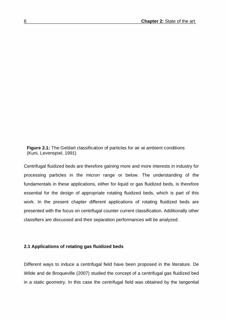
Geldart distinguished between four main categories of fluidizing behavior, taking the
density difference between particles and fluid and the mean particle diameter into
account, which are shown in the Geldart chart for beds fluidized with air at ambient
conditions (figure 2.1). Geldart A and B beds are strongly bubbling and Geldart D beds
can also spout when they are fluidized.
With decreasing diameter cohesion forces gain more and more influence on the
behavior of the fluidized bed and interparticle forces are greater than those resulting
from the action of the fluid. These beds are extremely difficult to fluidize and are
classified as Geldart C beds. Geldart C beds usually exhibit channeling, plugging and
the formation of “rat holes” (Watano et al., 2003).
With increasing interest in processing powders in the micron range (Geldart C) and
below, the application of a fluidized bed with its benefits like enhanced heat, mass
transfer or good handling due to fluid like behavior has a great potential in industrial
applications. One possibility to fluidize these particles is the transfer into the centrifugal
field. The replacement of the gravity by centrifugal acceleration allows the usage of
such higher fluid velocities compared to the gravity field.
6 Chapter 2: State of the art
Figure 2.1: The Geldart classification of particles for air at ambient conditions (Kuni, Levenspiel, 1991)
Centrifugal fluidized beds are therefore gaining more and more interests in industry for
processing particles in the micron range or below. The understanding of the
fundamentals in these applications, either for liquid or gas fluidized beds, is therefore
essential for the design of appropriate rotating fluidized beds, which is part of this
work. In the present chapter different applications of rotating fluidized beds are
presented with the focus on centrifugal counter current classification. Additionally other
classifiers are discussed and their separation performances will be analyzed.
2.1 Applications of rotating gas fluidized beds
Different ways to induce a centrifugal field have been proposed in the literature. De
Wilde and de Broqueville (2007) studied the concept of a centrifugal gas fluidized bed
in a static geometry. In this case the centrifugal field was obtained by the tangential

Chapter 2: State of the art 7
injection of the fluidizing gas via multiple gas inlet slots in the outer wall of the fluidizing
chamber.
A more common approach of centrifugal fluidization is the one in a rotating frame, i.e.
the whole system including the distributor is rotating at the desired angular velocity.
Qian et. al.,(2004) applied the fluidized bed in a horizontally rotating frame as a dust
filter for diesel exhaust gas treatment, where the unwanted soot particles are captured
in the fluidized bed. The advantage of the rotating fluidized bed for this application is
the reduction of the pressure drop compared to other types of granular bed filters. The
formation of bubbles and the bubble size development was studied and modeled by
Nakamura et. al.(2007), who found a reduction of bubble size with increasing
centrifugal acceleration in the rotating fluidized bed.
Figure 2.2: Rotating fluidized bed by Watano et. al. (2003)
Watano et. al. developed a rotating fluidized bed as shown in figure 2.2 for the
purposes of granulation (2003) and coating (2004). They fluidized highly cohesive

8 Chapter 2: State of the art
cornstarch powder with a median diameter of 15 m and obtained uniform fluidization.
The feasibilities of the granulation and the coating of micro particles due to the
centrifugal acceleration were demonstrated.
2.2. Wet classification in stationary classifiers
For processing particles with a desired range in size or density the use of classification
processes, i.e. the separation of a particle collective into a coarse and fines fraction, is
unavoidable. Dry classification is normally performed by air classifiers or sieves, for
the wet classification the most common classifier is the counter current classifier or
elutriator.
2.2.1 The principle of gravity elutriation
The principle of a gravity elutriator is shown in figure 2.3. The suspension is introduced
into the classifier from the top. While the particles are settling in the gravity
environment, the fluid phase of the suspension and additional injected water through
the distributor are forming an upstream, which is directed against the particles’ settling
velocities. As smaller particles are settling slower than larger particles, the presence of
suspensionfeed
fines
fluidizedbed
distributor
water coarse
classificationzone
Figure 2.3: Gravity elutriator (Schmidt, 2004)

Chapter 2: State of the art 9
an upstream is causing classification by taking the fines to an overflow weir, while the
coarse particles are settling in the direction of the distributor. The coarse particles are
accumulating in a bed, which is fluidized by the water injected through the distributor.
An intense movement of particles inside the fluidized bed is causing agglomerates to
decompose (Kalck, 1990), the emerging fines are carried out of the bed with the
upstream to the weir.
Elutriators can be operated continuously and high separation performances can be
achieved. The performance of the classification can be characterized by the
separation efficiency curve T(dp), which denotes the ratio of the coarse recovery to the
feed mass flow for a particle diameter dp. The characterization of the classification
performance is discussed in detail in chapter 5.7.
particle size [m]
sep
ara
tion
effi
cien
cy [%
]
Figure 2.4: Typical separation efficiency curves of gravity elutriation for sand (Heiskanen, 1993)
Typical separation efficiency curves are presented by Heiskanen (1993) in figure 2.4
for sand with cut sizes above 70 m. The presented curves show a sharp
classification, as it is desired for a classification process. Due to the reliability, the
classification performance and the low costs, the elutriator is widely used in industry.

10 Chapter 2: State of the art
Unfortunately, with decreasing particle diameter, the throughput is reduced or
alternatively, the elutriator’s diameter is increased to unacceptable high values at small
cut sizes, whereby the gravity elutriator is not applicable for classification tasks in the
micron range.
2.2.2 Classification with hydrocyclones
Wet classification for cut sizes in the
micron range can be enabled by the
enhancement of the settling velocities by a
centrifugal field. A very common
apparatus for this purpose is the
hydrocyclone, which is sketched in figure
2.5. The hydrocyclone consists of a
cylindrical part with the feed injection and
overflow at the top and a conical part with
coarse discharge at the bottom. The feed
is tangentially injected, which induces a
downward oriented vortex in the wall region. In the conical part an upward oriented
vortex at the center of the cyclone is achieved by the constriction of the cross sectional
area. The flow is then leaving the cyclone at the overflow. Due to the centrifugal force
the coarse particles are carried along the outer vortex at the wall and are then
discharged at the underflow, while the fines are able to follow the flow to the overflow.
Hydrocyclone classifications are normally applied for cut sizes between 5 and 250 m
(Kerkhoff, 1996). The popularity of the hydrocyclone is based on its low costs and its
high throughput at a low place requirement. The main disadvantages are the high
energy requirement and the sensitivity to clogging and unsatisfactory separation
performance (Kerkhoff, 1996). Especially the occurrence of the “fishhook effect”
(Majumder et. al., 2003), i.e. the recovery of fine particles in the hydrocyclone
underflow
feed
overflow
Figure 2.5: Principle of a hydrocyclone

Chapter 2: State of the art 11
underflow increases with decrease in particle size, is a major problem for hydrocyclone
classification tasks.
Figure 2.6 shows a typical separation efficiency curves of a hydrocyclone classification
with quartz (Gerhart, 2001) in the fines region, where a distinct “fishhook effect”
occurs. The reason for the “fishhook effect” is not really clarified yet, imprecise particle
size analysis, different densities of aggregates in the feed, flocculation of fines and the
dragging of fines to the underflow by coarse particles are discussed in the literature
(Gerhart, 2001). The separation efficiency of hydrocyclones in the micron range is
therefore not satisfying, so that other approaches have to be considered.
Figure 2.6: Typical separation efficiency curve of hydrocyclone classification (Gerhart, 2001) (hydrocylclone diameter: 39mm, pressure drop: 1.5 bar; material: quartz)
0
0.1
0.2
0.3
0.4
0.5
0.6
0.7
0.8
0.9
1
1 10 100particle size [m]
T [
-]
2.3 Wet centrifugal classification in rotating classifiers
Another possibility to create a centrifugal field is to rotate the whole apparatus. The
most common application is the centrifuge, which is often employed for classification
or dewatering tasks. For continuous operations decanter centrifuges are used (figure
2.7), in which the sediments are carried by a conveyer screw to the outlet (Stieß,
1993). In the literature classifications are reported with cut sizes down to 10 m

12 Chapter 2: State of the art
(Kellerwessel, 1979). Unfortunately, these centrifuges cause a strong compaction of
the sediment and fines are likely to be misclassified with the sediment to the coarse
discharge, what is not appropriate for industrial applications (Schmidt, 2004). An
apparatus, which is often used in industry for liquid-solid separation is the disc-stack
centrifuge. The principle is illustrated in figure 2.8 (Wang et. al, 1997). A suspension is
introduced at the center, from there the suspension is distributed to the rotating
chamber, where the separation takes place.
Figure 2.7: Principle of a decanter centrifuge (Stieß, 1993)
solids discharge(coarse)
feed
water with fines
The coarse particles are settling to a coarse discharge nozzle, while the fluid is
deflected and flowing versus the centrifugal force to the fluid outlet as pictured in figure
2.8. If disc-stack centrifuges are operated as classifiers it is unavoidable, that fines are
following the coarse particles instead of the fluid at the turnaround point. This leads to
a huge amount of misclassified fines (Schmidt, 2004).
For separation tasks for small cut sizes spinning wheel separators are often employed.
The principle is pictured in figure 2.9. The suspension is introduced (1) into a non
rotating chamber with a spinning wheel (4) inside. The fluid is passing through the
wheel versus the centrifugal acceleration in direction to the center. The centrifugal

Chapter 2: State of the art 13
acceleration is forcing the coarse particles back to outer chamber (2) from which the
coarse particles are discharged. The fines reaching the centre are then discharged
with the fluid (3). A problem of this principle is that the shear forces at the transition
from the non – rotating chamber to the wheel may cause breakage or attrition of the
particles. Another disadvantage is an unavoidable bypass of fines to the coarse
feedoverflow(fines)
underflow(coarse)
feedoverflow(fines)
underflow(coarse)
Figure 2.8: Principle of a disc stack centrifuge (Wang et. al, 1997)
Figure 2.9: Principle of a spinning wheel separator (Schmidt, 2004)
feed
fines
coarse
top view

14 Chapter 2: State of the art
fraction. Figure 2.10 shows a separation efficiency curve of such a classification. A cut
size of 8 m was reached, but a large amount of fines were misclassified, what is
indicated by the fishhook effect in the range below 4 m.
Figure 2.10: Separation efficiency of a soil classification with a spinning wheel separator (AHP 63, Hosokawa Alpine AG, Augsburg, Germany)
0
0.1
0.2
0.3
0.4
0.5
0.6
0.7
0.8
0.9
1
1 10particle size [m]
T [
-]
100
2.4. Classification from centrifugal fluidized beds
The devices presented above are capable for dewatering tasks and for the depletion of
a sharp fines fraction. When coarse fractions without fines are required the presented
classifiers show unacceptably strong fishhook effects. As the gravity elutriator is a
mature technology for reliable and sharp classification tasks, approaches were made
to transfer this technology to the micron range by applying a centrifugal field.
2.4.1 The principle of centrifugal elutriation
The principle of a centrifugal elutriator is the similar to the gravity elutriator. A particle
collective is settling versus a counter current flow at different settling velocities, which
are depending on the particle diameter. As smaller particles are settling slower than

Chapter 2: State of the art 15
larger particles a separation takes place when some particles are settling slower than
the velocity of the counter current. The gravity is replaced by a centrifugal force, which
can be orders of magnitude higher than the gravity, whereby particles in the micron
range can be classified. In contrast to gravity elutriation the centrifugal force is varying
with the radius and the flow pattern is influenced by the Coriolis force (Margraf and
Werther, 2008) acting perpendicular to radial direction.
For the illustration of centrifugal elutriation a radial force balance on a settling particle
can be applied (figure 2.11). The particle, when settling stationary, is experiencing a
centrifugal force FC, a buoyancy force FB and a drag force FD. The gravity force FG can
be neglected, when FG << FC is valid. This applies for the operation of the classifier in
this work. For spheres the following definitions are valid:
Centrifugal force: FC = S . /6 . dp3 . 2 . r (2.1)
Buoyancy force: FB = - L . /6 . dp
3 . 2 . r (2.2)
Drag force: FD = - cD(Rep) . /8 . dp
2 . L . vR
2, (2.3)
with the densities of the particles and the liquid S, L, the particle diameter dp and the
radial fluid velocity vR and the angular velocity .
FD FB
FC
Figure 2.11: Radial forces acting on a stationary settling particle in a centrifugal field
FD: drag force FB: buoyancy force FC: centrifugal force

16 Chapter 2: State of the art
A particle is theoretically floating at a constant radius in the upstream, when the sum of
the radial forces equals zero.
FB + FC + FD = 0 (2.4)
In the Stokes range the drag coefficient cD is defined:
cD = 24/Rep (2.5)
With (2.5) the drag force FD can be expressed by:
FD = - 3 . . . vR . dp , (2.6)
where denotes the viscosity of the fluid.
The radial fluid velocity vR can be expressed by:
RC
Vv
A
(2.7)
In equation (2.7) denotes the liquid volume flow and AC the cross sectional area at
the radius r. For the theoretical cut size dC, for which the radial fluid velocity equals the
particle settling velocity, it holds:
V
C 2C S L
V 18d
A ( )
r (2.8)
2.4.2 Centrifugal upstream classifiers
Preliminary studies to employ centrifugal counter current classification for cut sizes in
the micron range were published by Colon (Colon et. al., 1970). Colon developed two
prototypes, which are pictured in figures (2.12) and (2.13). The classification chamber
in the first prototype (figure 2.12) is a segment of the rotor. The suspension is
introduced in the center of the rotor (1) and then accelerated in 2 channels to the
speed of the rotor. In the classification chambers the suspension is then channeled to
the outer radius of the classification chamber and then turned back in direction of the

Chapter 2: State of the art 17
center. The fines are carried to the outlet (3), while the coarse particles accumulate in
the fluidized bed. A non rotating housing collects the fluid and the fine particles. They
are discharged at the outlet (2). The accumulated coarse particles in the classification
chamber have to be removed periodically.
Figure 2.12: Centrifugal classifier by Colon (1970) – Prototype I
Figure 2.13: Centrifugal classifier by Colon (1970) – Prototype II
The second prototype (figure 2.13) can be operated continuously. The suspension is
fed into the classification chamber at position (1), from where it is channeled to the
classification chamber. Additional water is introduced at (4), which causes a counter
current in the classification chamber. The coarse particles are settling versus the

18 Chapter 2: State of the art
centrifugal force and are discharged at the outlet (2). The fines are taken with the
current to the overflow (3). Colon successfully performed classifications with glass
beads for cut sizes down to 3 m (Schmidt, 2004). However, the achieved throughput
lies in lab scale dimension and is therefore not applicable for industrial purpose.
Priesemann (1994) designed a centrifugal upstream classifier with a circumferential
classification chamber, where the chamber width is expanding with decreasing radius
to assure a constant cut size over the chamber height. The classifier has to be
operated batch-wise, the experimental setup is pictured in figure 2.14. The suspension
is introduced into the classifier via a hollow shaft (1) and then channeled to the
classification chamber (5) by four pipes with nozzles (2) at the end. For the generation
of a counter current, additional water is injected to a ring chamber (3) at the outer
radius of the classifier. The water is passing a porous sinter metal distributor and
fluidizes the particles in the classification chamber. The fluidizing water with the fines
fraction is leaving the classifier via eight pipes (6). The coarse fraction is accumulating
in the fluidized bed and has to be removed, when a certain bed mass is reached.
Priesemann reached sharp classifications with cut sizes down to 4 m, but still with a
large amount of fines been misclassified. Figure 2.15 shows a separation efficiency
curve of Priesemann with a suspension volume flow of 52 l/h and a centrifugal
acceleration of 200g with quartz as solid feed. The diameter of the classification
chamber at the distributor level was 200 mm. The separation efficiency curve looks a
bit strange with a fishhook between 0.7 and 3m and an ideal classification below 0.6
m.
Based on the findings of Priesemann, Timmermann (1998) designed a continuously
operating centrifugal fluidized bed classifier for a higher throughput ratio. Contrary to
Priesemann the classification chamber is not circumferential, but consisting of closed
chambers. The rotor with a diameter of 200 mm can be rotated between 300 and 3000
rpm resulting in a range of centrifugal accelerations between 100 to 1000 times the

Chapter 2: State of the art 19
gravity acceleration. Cut sizes down to 0.5 m are possible at a suspension volume
flow up to 180 ml/min.
Figure 2.14: Setup of the centrifugal classifier of Priesemann (1994)

20 Chapter 2: State of the art
sepa
ratio
n ef
ficie
ncy
[%]
particle size [m]
Figure 2.15: Separation efficiency curve of the centrifugal classifier by Priesemann (1994)
Figure 2.16 shows two cuts through the classification chamber of the apparatus of
Timmermann (1998). Four suspension injection nozzles (1) are installed in the
classification chamber and are fed with suspension from a hollow shaft. The fluidizing
water is introduced to the apparatus at (2) and flows through a porous distributor (3),
behind which it fluidizes the bed consisting of the coarse fraction. The coarse particles
can be discharged by a suction tube (5) which is submerged in the fluidized bed during
operation. It has to be mentioned that the suction velocity at the coarse discharge has
to be higher than the settling velocity of the coarse particles. The fines are taken with
the fluidizing water to the overflow (4), where they get discharged. Under this condition
a high volume flow is passing through the coarse discharge pipe leading to a high
dilution or low solids concentration in the coarse suspension. Timmermann reports in
his work about comparable results like Priesemann in her batch experiments, but with
continuous operation. For an industrial application the throughput (0.0006 – 0.019
m3/h) and the separation efficiency are still not sufficient.

Chapter 2: State of the art 21
Figure 2.16: Setup of the centrifugal classifier of Timmermann (1998)
cut B – B’
cut A – A’
As the above presented classifiers do not show satisfactory results for classification in
the micron range with throughputs adequate for industrial application, Schmidt (2004)
designed a centrifugal counter current classifier, which is also the equipment of the
present work. The principle is shown in figure 2.17. Like in a gravity elutriator the
suspension is fed into the classification chamber where the settling of the particles is
hindered by a counter current flow. The insertion of the suspension and the fluidizing
water is realized by rotary feedthroughs to the hollow shafts in the axis. The fines are
carried by the current to an overflow weir, while the coarse fraction is forming the
fluidized bed, from where the coarse particles are discharged. The centrifugal force
can be adjusted to exceed the gravitational force by orders of magnitudes to enable an
appropriate settling of particles in the micron range.

22 Chapter 2: State of the art
Figure 2.17: Principle of the centrifugal counter current classifier (Schmidt, 2004)
The target of Schmidt’s work was to design a classifier with the same separation
efficiency like a gravity elutriator but with cut sizes down to few microns. On the
contrary to the above presented prototypes the classifier of Schmidt is designed for
suspension throughputs between 137 – 1900 l/h, which lies in the range of industrial
demand (Schmidt, 2004). The rotor has a diameter of 1m and a circumferential
classification chamber. The advantage of a circumferential classification chamber is
the fact that a complete revolution, i.e. 360° of the rotor, is used for the separation.
With a distributor area of 0.05592 m2 the dimensions of the classifier are much larger

Chapter 2: State of the art 23
compared to those of Timmermann (1998) and Priesemann (1994). The principle of
the chamber profile is based on the condition that the cut size has to be constant over
the chamber height. As the cut size depends on the radial position in the classification
chamber, the radial velocity has to be varied above the chamber height to maintain a
constant cut size. Applying equation (2.8) leads to the conclusion that the ratio of the
radial velocity and the radius has to be constant. The condition of constancy of the cut
size was realized by Schmidt (2004) due to the design of the classification chamber.
According to Schmidt (2004) the existence of a fluidized bed is required for de-
agglomeration and therefore the control of the bed height is one of the key tasks for
the operation of the classifier. Schmidt selected needle valves operated with an elbow
lever mechanism for the bed height control, which is presented in detail in chapter 3.
Schmidt conducted experiments to characterize the influences of the angular speed,
the suspension to fluidizing water ratio and the influence of the suspension solids
content. The experimental materials limestone and quartz with similar properties
compared to the ones of the present work, were used by Schmidt. For the analysis of
the particle size distributions a laser diffraction analyzer (Type HELOS 12 KA/LA,
Sympatec Germany) was applied using the Fraunhofer model for evaluation.
The investigation of the influence of the angular velocity at a constant theoretical cut
size (equation 2.8) was conducted by varying the water throughput depending on the
angular velocity. Schmidt (2004) found that with increasing angular velocities the
separation efficiency curves are shifted to larger particle diameters and the “fishhook
effect” is reduced. Figure 2.18 shows a separation efficiency curve of limestone
classification for different angular speeds at a fluidizing to suspension flow ratio of 2:1.
Further experiments were conducted to describe the influence of the fluidizing to
volume flow ratio on the separation efficiency. Schmidt found that an increase of the
ratio results in a higher separation efficiency and in a reduction of the fishhook. This
can easily be seen in figure 2.19, where the fluidizing to suspension flow ratio was

24 Chapter 2: State of the art
se
para
tion
effi
cie
ncy
[-]
theoretical cut size: 6 m
particle diameter [m]
Figure 2.18: Influence of the angular speed on the separation efficiency (Schmidt, 2004)
sepa
ratio
n ef
ficie
ncy
[-]
theoretical cut size: 6 m400 rpm
particle diameter [m]
Figure 2.19: Influence of the fluidizing to suspension flow ratio on the separation efficiency (Schmidt, 2004)

Chapter 2: State of the art 25
varied for the classification of limestone at 400 rpm for a theoretical cut size of 6 m.
An influence of the feed solids concentration was studied as well, but Schmidt (2004)
found no significant influence of the solids concentration on the separation
performance.
Comparing the calculated cut sizes (equation 2.8) with the results of the experiments,
Schmidt (2004) discovered an underestimation of the theoretical cut sizes, i.e. the
measured cut sizes were almost always higher than the calculated ones. This is
revealed in figure 2.20, where the measured cut sizes are plotted versus the
calculated ones. Schmidt (2004) explained the deviation due to the occurrence of
swarm settling instead of single particle settling in the classification zone of the
freeboard, which was assumed in his model. The swarm settling leads to a reduction
of the particle settling velocities, whereby the deviation of the calculated cut sizes to
the experimental findings can be explained.
Although with the design of Schmidt (2004) cut sizes below 10 m were successfully
reached, the sharpness of the classification was not satisfactory. Furthermore the
separation efficiency curves by Schmidt revealed a strong “fishhook effect”, which
could not be eliminated with the actual configuration of the classifier.
However, the principle of centrifugal elutriation has a high potential to fulfill the
industrial demand for wet classification in the micron range. The classifier of Schmidt
reaches the desired cut sizes as well as suspension throughputs for industrial
applications. The elimination of the fishhook and the increase of the sharpness are
therefore the key tasks for optimization. A problem with the classifier of Schmidt is that
the needle valves, which are operated with an elbow lever mechanism, are not
capable to control the bed height accurately. Another problem is the flushing out of the
bed material, which lead to misclassification through bypassing of fines to the outlet.

26 Chapter 2: State of the art
Thus there is a lot of potential for optimization. Therefore the understanding of the
fundamentals of the fluid mechanics and the wet centrifugal fluidization are essential.
These fundamentals are not completely understood yet, so that their investigation is
one of the key points of the present work.
Figure 2.20: Comparison of the theoretical and experimental cut sizes (Schmidt, 2004)
dc [m] - measured
d c[
m] -
calc
ulat
ed
In the following simulations of the pure liquid flow in a rotating chamber (i.e. according
to the conditions in the solids-free chamber or in the freeboard of the fluidized bed,
respectively) with the CFD software CFX will be performed and experiments will be
carried out to verify the findings of the simulation and to describe the behavior of the
fluidized bed. The characterization of the fluidized bed behavior will be conducted by
the determination of its expansion and the pressure drop profile under different angular
velocities. From the findings the classifier will be improved, especially an improvement
of the coarse discharge is considered in this work, which plays an important role for
the control of the bed height.
3 Setup and design of the centrifugal fluidized bed
classifier
In this chapter the setup of the classifier is presented, which is based on the previous
work conducted by Schmidt (2004). The general data of the classifier are provided as
well as a detailed explanation for the design of the classification chamber. The coarse
discharge mechanism of Schmidt (2004) is presented, which plays an important role in
separation performance. The coarse discharge is modified later, which is part of
chapter 5.
3.1 Experimental setup
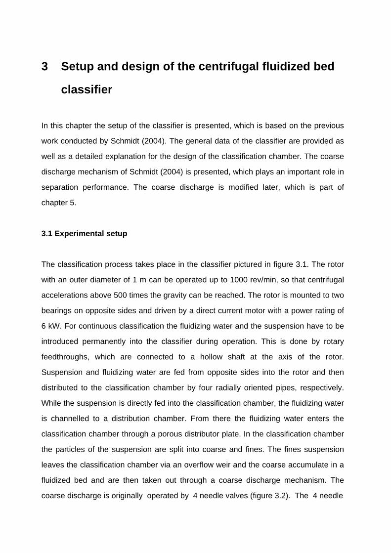
The classification process takes place in the classifier pictured in figure 3.1. The rotor
with an outer diameter of 1 m can be operated up to 1000 rev/min, so that centrifugal
accelerations above 500 times the gravity can be reached. The rotor is mounted to two
bearings on opposite sides and driven by a direct current motor with a power rating of
6 kW. For continuous classification the fluidizing water and the suspension have to be
introduced permanently into the classifier during operation. This is done by rotary
feedthroughs, which are connected to a hollow shaft at the axis of the rotor.
Suspension and fluidizing water are fed from opposite sides into the rotor and then
distributed to the classification chamber by four radially oriented pipes, respectively.
While the suspension is directly fed into the classification chamber, the fluidizing water
is channelled to a distribution chamber. From there the fluidizing water enters the
classification chamber through a porous distributor plate. In the classification chamber
the particles of the suspension are split into coarse and fines. The fines suspension
leaves the classification chamber via an overflow weir and the coarse accumulate in a
fluidized bed and are then taken out through a coarse discharge mechanism. The
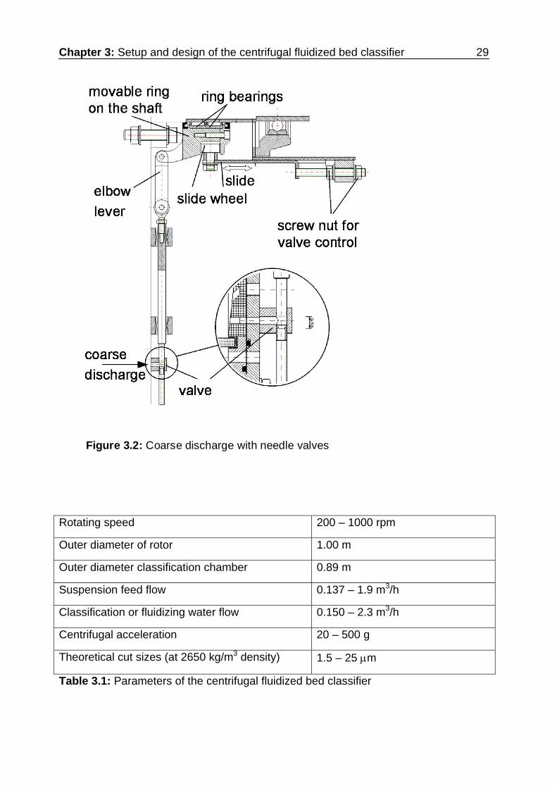
coarse discharge is originally operated by 4 needle valves (figure 3.2). The 4 needle

28 Chapter 3: Setup and design of the centrifugal fluidized bed classifier
Figure 3.1: Design of the centrifugal fluidized bed classifier
non – rotating particle capture chamber
distributor
rotaryfeedthrough
rotaryfeedthrough
bearingbearing
distributorchamber
shaft
overflow weir
fines coarse
elbow lever
slide for elbowlever control
valves are connected with an elbow lever mechanism to a ring, which can be moved
on the shaft. A non-rotating slide with a wheel running in the ring enables the
movement of the ring, which opens or closes the needle valves. The coarse discharge
mechanism has a strong influence on the performance of the classifier and will be
modified later according to the findings of the investigation of the fluid (chapter 5). The
coarse and the fines are captured in a non-rotating ring chamber made of plexiglass.
The ring chamber is divided into two sections, one for the coarse, the other one for the
fines fraction. The fines and the coarse suspension leave the ring chamber at the
bottom from opposite sides. Photographs of the classifier are shown in figure 3.3 (left:
frontview; right: backview). The operational parameters are summarized in table 3.1
(Schmidt and Werther, 2005).
Chapter 3: Setup and design of the centrifugal fluidized bed classifier 29
Figure 3.2: Coarse discharge with needle valves
Rotating speed 200 – 1000 rpm
Outer diameter of rotor 1.00 m
Outer diameter classification chamber 0.89 m
Suspension feed flow 0.137 – 1.9 m3/h
Classification or fluidizing water flow 0.150 – 2.3 m3/h
Centrifugal acceleration 20 – 500 g
Theoretical cut sizes (at 2650 kg/m3 density) 1.5 – 25 m
Table 3.1: Parameters of the centrifugal fluidized bed classifier
30 Chapter 3: Setup and design of the centrifugal fluidized bed classifier
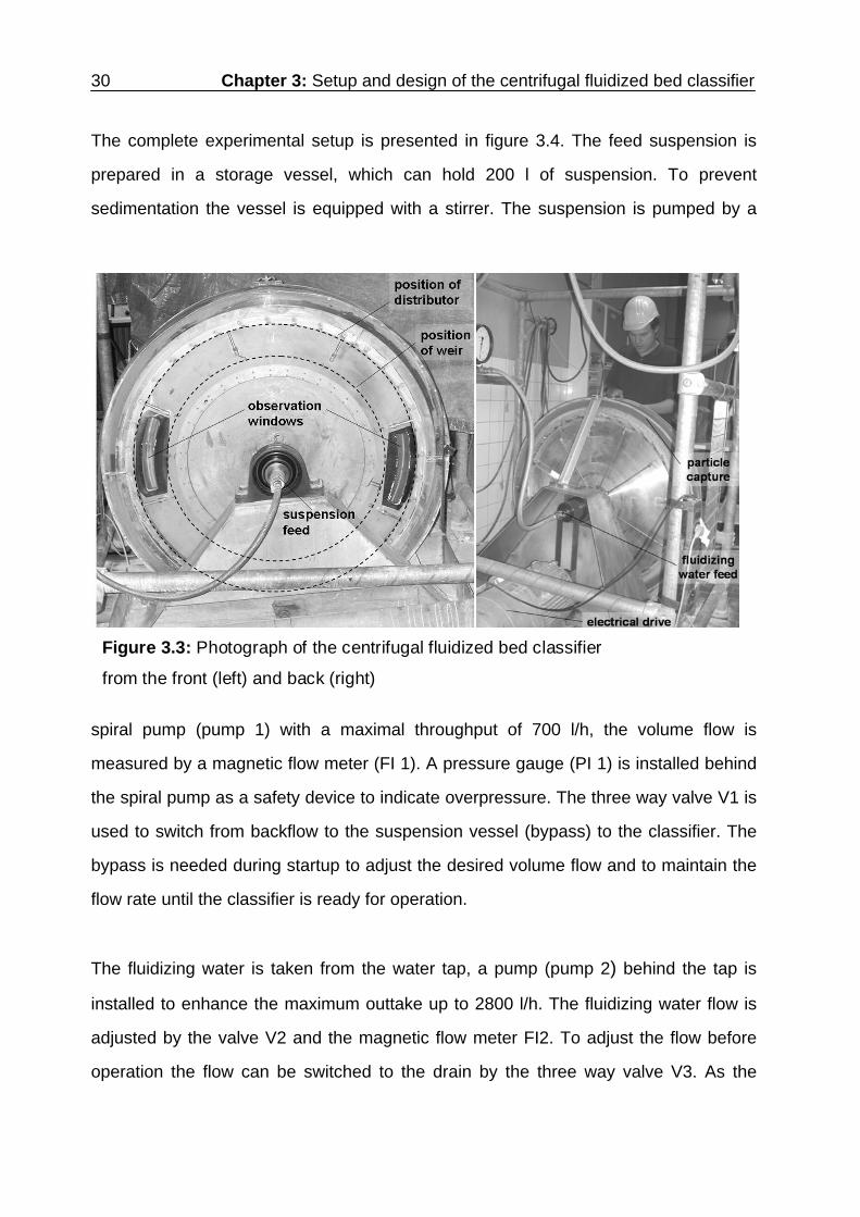
The complete experimental setup is presented in figure 3.4. The feed suspension is
prepared in a storage vessel, which can hold 200 l of suspension. To prevent
sedimentation the vessel is equipped with a stirrer. The suspension is pumped by a
Figure 3.3: Photograph of the centrifugal fluidized bed classifier
from the front (left) and back (right)
spiral pump (pump 1) with a maximal throughput of 700 l/h, the volume flow is
measured by a magnetic flow meter (FI 1). A pressure gauge (PI 1) is installed behind
the spiral pump as a safety device to indicate overpressure. The three way valve V1 is
used to switch from backflow to the suspension vessel (bypass) to the classifier. The
bypass is needed during startup to adjust the desired volume flow and to maintain the
flow rate until the classifier is ready for operation.
The fluidizing water is taken from the water tap, a pump (pump 2) behind the tap is
installed to enhance the maximum outtake up to 2800 l/h. The fluidizing water flow is
adjusted by the valve V2 and the magnetic flow meter FI2. To adjust the flow before
operation the flow can be switched to the drain by the three way valve V3. As the

Chapter 3: Setup and design of the centrifugal fluidized bed classifier 31
desired flow is reached V3 can be the switched to the classifier. A pressure gauge
(PI2) indicates the pressure in front of the fluidizing water feedthrough.
Figure 3.4: Experimental setup
3.2 The geometry of the classification chamber
The most important part is the circumferential classification chamber, where the split of
the suspension into coarse and fines takes place. The design and the dimensions of
the classification chamber are shown in figure 3.5.
Figure 3.5: Drawing (left) and sketch (right) of the classification chamber
RD = 445 mm
RW = 335 mm
RD = 445 mm

32 Chapter 3: Setup and design of the centrifugal fluidized bed classifier
The suspension is injected to the classification chamber by 4 ports, 30 mm above the
distributor at an angle of 45°. The injected particles inside the chamber are affected by
a counter current, which causes the classification effect. While the coarse particles
accumulate in the fluidizing bed, the fines are carried with the radial flow to the
overflow weir. The fluidizing water is distributed across the circumference by a ring
chamber and enters the classification chamber through a 8 mm thick porous distributor
(CELLPOR – TYPE 152, Porex Technologies GmbH, Singwitz, Germany). The
distributor has a linear pressure drop characteristics up to a fluid velocity of 0.02 m/s.
The pressure drop at 0.02 m/s is 0.42 bar.
The classification chamber is equipped with two windows made from plexiglass (cf.
figure 3.3), which enables the observation of the fluidized bed and particularly its
freeboard with the help of a stroboscope and a high-speed camera (KODAK
EKTAPRO). The camera is able to take up to 1000 frames per second.
The cut size dC, i.e. the condition where the drag on a single particle equals the
centrifugal force minus the buoyancy force is one of the most important aspects of
classification. It determines the profile of the classification chamber and the operating
conditions. Inserting the cross sectional area AC, with
AC = 2 . r . B; (3.1)
and with the chamber width B, into equation (2.8), it follows:
C 2S L
18 Vd
( ) r 2 r
B (3.2)
As a constant cut size is desired for all radial positions the product r2*B must be kept
constant. Therefore the width B of the chamber has to be reduced with increasing

Chapter 3: Setup and design of the centrifugal fluidized bed classifier 33
distance from the axis. The resulting parabolic profile was approximated by two linear
sections to facilitate manufacturing of the classification chamber (cf. figure 3.5). The
deviation of the approximated chamber profile from the ideal profile was always below
2% (Schmidt 2004) and thus the assumption of a constant cut size over the chamber
height is valid.
4 Theory
With the centrifugal fluidized bed classifier a novel system was designed to perform
particle separation in the micron range. The classification takes place in a
circumferential classification chamber, in which the fluid and the bed can freely move
in tangential direction. The fluid enters the chamber in radial direction at the distributor
(radial position of the distributor: RD = 0.445 m) and leaves it at the weir (radial position
of the weir: RW = 0.335 m). The centrifugal acceleration varies with the distance from
the axis and furthermore the flow is affected by the Coriolis force, which reaches high
values at high angular speed rates.
The Coriolis force describes the influence of the rotation on an object in motion in a
rotating reference frame. The Coriolis force is proportional to the speed of rotation and
to the mass and the velocity of the object. The Coriolis force acts in a direction
perpendicular to the rotation axis and to the velocity of the object in the rotating frame.
The Coriolis force vector is defined: corS
corS 2m
U, (4.1)
where m is the mass of the object,
the angular velocity vector and U the velocity
vector of the object in the rotating reference frame.
Little research was done in the past to describe a flow in such a system. Schmidt
(2004) assumed the Coriolis force to be negligible and conducted CFD – simulations
for pure liquid flow without the Coriolis force. His results showed a radially oriented
flow pattern, which was only influenced by the suspension injection ports.
As the Coriolis force acts perpendicular to the centrifugal force, i.e. in tangential
direction, it can be expected, that the Coriolis force has a significant influence on the
flow pattern in the annular chamber. A significant influence of the Coriolis force would

Chapter 4: Theory 35
induce a velocity component in tangential direction. These expectations are contrary to
Schmidt’s (2004) assumptions and have to be investigated. In this chapter the theory
of the computational investigation of the single phase liquid flow (water) is presented.
For a rough estimation a simplified model was developed and the results are
compared with a precise CFD simulation with the software CFX 5.7.
4.1 A simplified hydrodynamic model of the liquid flow in the solids-free
chamber (model I)
The model presented in this section describes the induction of tangential movement
relative to the wall from the distributor in the direction to the overflow weir. The
observer in this model is located outside, i.e. the velocity of the rotor is as well
considered as the tangential flow.
The principle underlying this model is to apply the conservation of angular momentum
(Dixon, 1998) on a ring element with the thickness dr. The massflow passes the
ring element with the thickness dr in radial direction (figure 4.1). For the momentum
balance the angular momentum MF of the flow into the element, the angular
momentum MO of the flow out of the element and the torque MW caused by wall friction
have to be considered. The viscous momentum transfer between ring elements is
neglected, since the velocity gradient between the walls is much higher than from the
distributor to the weir and therefore the radial viscous momentum transfer is
considered to be small compared to the wall friction. Conservation of angular
momentum on a ring element with thickness dr means
m
Wm (w dw) (r dr) M m w r 0 , (4.2)
where is the fluid mass flow, w the absolute tangential velocity, r the radius and MW
the torque with regard to the axis.
m

36 Chapter 4: Theory
Transforming equation (4.2) results in:
Wm (r dw w dr) M (4.3)
The angular torque MW is a product of wall friction force FW and radius r,
MW = FW * r (4.4)
Figure 4.1: Balance of angular momentum on a ring element of the liquid in the classification chamber
The wall friction force can be derived from the pressure loss p for a through-flow
system (Bohl, 1991):
p = 0.5 * * L/dh * * vT2, (4.5)
where L is the circumference, dh the hydraulic diameter, vT the velocity of the fluid
relative to the wall and the wall friction coefficient.

Chapter 4: Theory 37
The pressure loss p equals the wall friction FW divided by the cross sectional surface
AQ.
FW = p . AQ (4.6)
The relative tangential velocity vT between the fluid and the wall is replaced by the
absolute velocity w of the fluid minus the velocity of the wall at the radial position r.
vT = w – r * , (4.7)
where r is the radial position and the angular velocity. It follows
FW = 0.5 * * L/dh * * AQ * (w – r * )2, (4.8)
The hydraulic diameter dh for slit flow (Schröder, 2004) results from the chamber width
B:
dh = 2 * B(r) (4.9)
It holds
AQ = B(r) * dr; (4.10)
and
L(r) = 2 * * r (4.11)
which leads for the wall friction force of the ring element to
FW = 0.5 * * * * (w – r * )2 * r * dr (4.12)
It follows for the torque
MW = 0.5 * * * * (w – r * )2 * r2 * dr (4.13)
Inserting equation (4.13) into equation (4.3) results in
2 2m (r dw w dr) 0.5 (w r ) r drl p r w⋅ ⋅ + ⋅ = ⋅ ⋅ ⋅ ⋅ - ⋅ ⋅ ⋅ (4.14)
which leads to
(4.15) WM mdw = w dr
m r
- ⋅ ⋅⋅

38 Chapter 4: Theory
or
(4.16) 2(d
l p r wé ⋅ ⋅ê -w r ) r ww dr
2 m r
ù⋅ ⋅ - ⋅ ú= ê ú⋅ë û
The calculation of profile of the tangential velocity along the height of the chamber was
conducted in the following way: the starting point of the calculation of the tangential
velocity distribution is at the distributor. At this point the tangential velocity of the fluid
equals the velocity of the apparatus, i.e. vT = 0 m/s.
D Dw(R ) R w= ⋅ (4.17)
With equation (4.16) the change w of the absolute tangential velocity of the fluid after
the distance -r can be calculated. With w from equation (4.16) the starting value for
the next iteration is then given by:
D Dw(r R r) w(r R ) w= -D = = +D (4.18)
The local relative tangential velocity vT(r) can be calculated as the difference between
the tangential velocity of the apparatus and the absolute tangential velocity of the fluid.
4.2 CFD simulation of the pure liquid flow (model II)
The CFD simulation is a complex Eulerian flow calculation and is used to predict flow
patterns. It is presently used to confirm the validity of the simplified model and to give
more detailed information about the flow behavior inside the classification chamber.
For this purpose the CFD software CFX 5.7 by ANSYS, Inc. was used. Due to
complexity a single phase model with water as liquid phase is considered only. This
chapter consists of two parts, the geometry and the CFD model part. In chapter 4.2.1
the geometry and the grid as well as cell types are presented. Chapter 4.2.2 describes
the equations to be solved in each cell of the domain and the turbulence model. The
domain is the body of the geometry, in which the fluid flow is calculated. The
calculation of the CFD model was conducted for an observer inside the system, i.e.

Chapter 4: Theory 39
only the velocities relative to the rotating reference frame are considered. The effect of
the rotation on the flow pattern is contributed by adding centrifugal and Coriolis force
terms to the Navier-Stokes equations.
4.2.1 Geometry and computational grid
Because a single-phase model is used only, the suspension feed and the coarse
discharge can be neglected for the determination of the flow pattern. For the
determination of a general tangential flow pattern this simplification is valid as the flow
through the distributor to the weir is much larger than the flow through the feed and
discharge ports. The modeling of the classification of particle collectives this way is too
inaccurate as local radial velocities in the near discharge and feed port regions play an
important role for classifications. Therefore simulations of classifications were not
conducted in this work. Neglecting the feed and discharge ports, the classification
chamber becomes completely rotational symmetric to the axis. Due to symmetry it is
possible to consider just a small section of the classification chamber for the CFD –
model. As the total amount of cells for this model was limited to approximately 300000
cells due to the available computing power, it is advisable to use a section less than
10° of the whole classification chamber to achieve a sufficient cell number in the
model. This enables a high mesh refinement, especially in the near wall region, where
high shear stresses occur. A higher number of cells would result in an unacceptably
high calculation time.
Figure 4.2 shows the domain of the model used for the calculation, which is defined as
a rotating reference frame, meaning that the calculated velocities are related to the
wall velocity. At the front and back of figure 4.2 the side walls are visible. The wall
surfaces are defined as no slip walls, i.e. the velocity is zero. The left and right
surfaces of the domain are modeled as periodic boundaries. Periodic boundary
condition means that a value transported over the periodic boundary will reenter the

40 Chapter 4: Theory
geometry at the corresponding other periodic boundary. The periodic boundary
condition is valid for a completely rotationally symmetric system. The shapes of the
periodic boundary surfaces are identical to the real chamber profile, like presented in
figure 3.5 (right), but without feed and coarse discharge.
opening
periodic boundary
periodic boundary
inlet
0.05 m
opening
periodicboundary
0.11
m
no slipwall
periodicboundary
Figure 4.2: Frame of the CFD model for the calculation of the liquid flow in the classification chamber
In the real chamber a porous distributor plate is used as water inlet. To simplify the
calculation and to increase the robustness of the solver the porous distributor is not
considered. Instead the inlet with a constant velocity in radial direction only is
assumed.
At the top of the chamber the fluid leaves the fluid domain. This boundary is modeled
as an opening with a relative pressure of 0 Pa. The opening boundary condition allows
the fluid to leave and also to enter the domain. Although only a flow out of the domain
is possible, the opening condition achieves a higher stability of the solver (CFX
Manual, 2004).

Chapter 4: Theory 41
Figure 4.3 shows the hexahedral mesh on the domain surfaces. A hexahedral mesh
was chosen, because the solver shows a faster convergence of the equation system
than with a tetrahedral mesh, what was tested on the domain of figure 4.2. Another
reason for using a hexahedral mesh is the fact, that a more effective mesh refinement
in the near wall region is achieved.
The refinement of the mesh in the wall region, where the highest velocity gradients
occur and shear stresses occur, can be seen in figure 4.3. A cell width of 0.1 mm in
that region is achieved, which is necessary for an accurate modeling. The whole grid
of the chamber consists of 236,811 hexahedron cells and has a height of 110 mm and
a width of 20 to 33 mm.
The geometry presented above is valid for a circumferential classification chamber, i.e.
the fluid can move freely in tangential direction. Previous works (Timmermann, 1998;
Priesemann, 1994) dealt with a closed classification chamber, i.e. the fluid is
surrounded by four walls while passing through the classification chamber. The
question arises, how the flow is influenced in a closed system by the rotational forces
in such a system. A simulation with a closed system can be easily carried out by
replacing the periodic boundaries of figure 4.2 by no slip walls. The fluid mechanics of
that system were also investigated in the present work.

42 Chapter 4: Theory
Fig
ure
4.3:
Hex
ahed
ralm
esh
of t
he
CF
D m
odel
in
let
surf
ace
no
slip
sur
face
op
enin
g su
rfac
e p
eri
od
ic b
ou
nd
ary
su
rfa
ce
Chapter 4: Theory 43
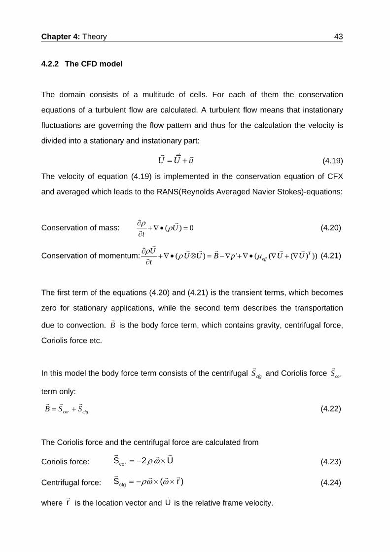
4.2.2 The CFD model
The domain consists of a multitude of cells. For each of them the conservation
equations of a turbulent flow are calculated. A turbulent flow means that instationary
fluctuations are governing the flow pattern and thus for the calculation the velocity is
divided into a stationary and instationary part:
U U u (4.19)
The velocity of equation (4.19) is implemented in the conservation equation of CFX
and averaged which leads to the RANS(Reynolds Averaged Navier Stokes)-equations:
Conservation of mass: ( ) 0
U
t (4.20)
Conservation of momentum: ( ) ' ( ( ( )
))
T
eff
UU U B p U U
t (4.21)
The first term of the equations (4.20) and (4.21) is the transient terms, which becomes
zero for stationary applications, while the second term describes the transportation
due to convection. B
is the body force term, which contains gravity, centrifugal force,
Coriolis force etc.
In this model the body force term consists of the centrifugal cfgS
and Coriolis force corS
term only:
cfgcor SSB
(4.22)
The Coriolis force and the centrifugal force are calculated from
Coriolis force: corS 2
U (4.23)
Centrifugal force: cfgS (
r ) (4.24)
where is the location vector and Ur
is the relative frame velocity.

44 Chapter 4: Theory
The second term on the right side of equation (4.21) is the momentum transfer by
pressure gradients. The third term on the right of equation (4.21) represents the
diffusive momentum transport by shear stresses. The shear stresses due to turbulence
is contained in the effective viscosity eff = + t, with the bulk viscosity and the
turbulent viscosity t.
The used k- model assumes that the turbulent viscosity is linked to the turbulent
kinetic energy k and turbulent frequency via the relation:
t = . k/ (4.25)
The starting point of the present formulation is the k- model developed by Wilcox
(Manual CFX 5.7, 2004). It solves two transport equations, one for the turbulent kinetic
energy, k, and one for the turbulent frequency, .
Turbulent kinetic energy:
(4.26)
tk
k
( k)( Uk) k P ' k
t
Turbulent frequency:
(4.27)
2t
k
( )( U ) ' P
t k
Pk is the turbulence production due to viscous forces, which is modelled using:
Tk t t
2P U ( U U ) U(3 U3 k)
(4.28)
The model constants are given by:
’ = 0.09; ’= 0.5556; = 0.075; k = 2; = 2
The equation system (4.19) – (4.28) is solved by the finite volume method in each cell
of the grid. Additionally, to compare the influence of the fluid a simulation with air was
conducted. In the simulations water (density = 999 kg/m3; dynamic viscosity =
0.0013 kg/m s at 10°C) and air at ambient conditions (density = 1.2 kg/m3; dynamic
viscosity = 0.0018 kg/m s) were used.

5 Experimental
In this chapter the techniques to measure the properties of the centrifugal fluidized bed
are presented. Particularly the measurement of the fluid dynamics is of major interest
to confirm the results of the simulation and to gain knowledge of the influence of the
particles in the fluid. As already mentioned in chapter 4 a strong velocity in the
circumferential direction is expected due to the Coriolis force. The available simulation
techniques only consider a single phase flow, so measurements are necessary to find
out about the influence of particles on the flow pattern. In this regard the methods to
determine the flow behavior of the freeboard and of the fluidized bed will be presented.
Furthermore the techniques for measuring the bed pressure drop and the expansion
behavior will be explained. The measurement and the modeling of the bed pressure
drop profile depending on the fluidizing velocity are important to find the limiting cut
sizes for classifications. The pressure drop profiles reveal the minimal fluidizing
velocities at given conditions, where the bed is stably fluidized. Below the minimum
fluidization point the operation of the classifier is not recommended as defluidized
zones reduce the classification performance or completely block the coarse discharge.
To model the pressure drop profile, the knowledge of the expansion behavior is
necessary. This enables the calculation of the bed height from the pressure drop and
allows an estimation of the flow through the modified coarse discharge. Other topics of
this chapter are the presentations of the coarse discharge modifications as well as the
analysis methods and the bed materials used in the experiments.
5.1 Experimental materials
For the experimental investigation of the centrifugal fluidized bed and for the
characterization of the classification performance suitable materials had to be chosen.
Limestone and quartz powder are often used for this purpose, because they are

46 Chapter 5: Experimental
cheap, available in many particle sizes and are not dissolvable or reactive in aqueous
media. With densities between 2500 kg/m3 and 3000 kg/m3 quartz and limestone are
good to handle and have adequate settling velocities for classification in the micron
range. Other advantages of limestone and quartz are that they are 99.9 % pure and
well studied, i.e. properties like the refraction index, which is important for the
determination of the particle size distribution by the laser diffraction analysis, are
documented in the literature. Thus they were used in this work. The quartz powder
(SF300, Quarzwerke Frechen, Frechen Germany) had as density of 2650 kg/m3 and a
refraction index of 1.54 (specification of the producer). Quartz was used for the
determination of the tangential bed movement, for the bed expansion and for
classification experiments. Limestone (Saxolith 10HE, Geomin, Hermsdorf/Germany)
with a density of 2620 kg/m3 and a refraction index of 1.59 was used for bed
expansion and classification experiments. Limestone and quartz are natural products
and have therefore irregular shapes. To compare the findings of the investigations of
quartz and limestone with spheres, glass beads (Strahlperlen 0-50 m, Strahlperlen
Auer GmbH, Mannheim/Germany) with a density of 2500 kg/m3 and a refraction index
of 1.50 were used for classification experiments and for the determination of the
expansion behavior. The particle size distributions of the used materials are shown in
figure 5.1 and photographs by a scanning electron microscope (SEM) in figure 5.2.
Figure 5.1: Cumulative mass (left) and mass density (right) distributions of the experimental materials quartz, limestone and glass beads
0102030405060708090
100
1 10 100particle size [μm]
Q3
[%
]
0
50
100
150
200
250
300
350
400
1 10 10particle size [μm]
q3
[%/μ
m]
0
50
100
150
200
250
300
350
400
0
quartz
limestone
glass beads

Chapter 5: Experimental 47
Figure 5.2: SEM pictures of quartz (top), limestone (center) and glass beads (bottom) at 2000x magnification

48 Chapter 5: Experimental
5.2 Flow measurement techniques in the rotating classification chamber
In this section the techniques to measure the flow in circumferential direction due to
the Coriolis force will be presented. First of all the measurement of the pure liquid flow
will be discussed and in the second part the determination of the movement of the
fluidized bed will be explained.
5.2.1 Pure liquid flow in the rotating classification chamber
The measurement of the flow velocity is a standard task in industry. The simplest form
to measure the velocity is the Pitot tube (John G. Webster, 1999). The basic Pitot tube
simply consists of a tube pointing directly into the fluid flow and the pressure can be
measured as the moving fluid is brought to rest. This pressure is the stagnation
pressure of the fluid, also known as the total pressure. The measured stagnation
pressure cannot of itself be used to determine the flow speed. However, since
Bernoulli's equation states that
Stagnation Pressure = Static Pressure + Dynamic Pressure
the dynamic pressure is simply the difference between the static pressure and the
stagnation pressure. The static pressure is generally measured using the static ports
on the side of the Pitot tube. From the dynamic pressure the flow speed can be
calculated. Other standard methods to determine the fluid velocity are impellers or
thermal mass flow sensors. The flow velocity measured by the impeller is calculated
by its rotational speed, when the fluid properties viscosity and density are known. The
thermal mass flow sensor uses the dependence of the heat transfer on the fluid
velocity, i.e. the higher the velocity the more heat is transferred. The heat transfer can
be measured and from it the fluid velocity can be calculated.
The methods described above require wiring for power supply and data transfer, what
is not a problem for standard applications in normal gravity environment. In a rotating
Chapter 5: Experimental 49
system wiring is not possible unless the data receiver and the power supply are
rotating with the system. Installing a rotating power supply and receiver brings an
unfavorable unbalance to the rotating system. Other problems are the high centrifugal
acceleration forces and the high pressure gradients in the system, an environment
where standard sensors are not designed and calibrated for.
For that reason it was necessary to think about a novel technique to measure the
tangential flow velocity, where no wiring is required and no unbalance is brought to the
rotor. The idea is to determine the velocity by a tracer, which is observed through the
vision panels of the rotor.
This was done with the help of spheres which were attached to a fixing 13.5 mm
above the distributor by a thread. The sphere and the thread are deflected from the
radial direction by a tangential flow. With the angle of deflection the tangential velocity
can be calculated by applying a force balance on the sphere. The principle of the
tangential flow measurement is presented in figure 5.3. Two spheres with diameters of
dts1 = 9.9 mm (volume Vts1 = 0.5 cm3) and of dts2 = 4.5 mm (volume Vts2 = 0.06 cm3),
respectively, were used. The sphere materials were plastics with the densities ts1 =
920 kg/m3 for the larger sphere and ts2 = 1200 kg/m3 for the small sphere. Thus the
first sphere was buoying towards the center while the second was sinking in the
direction of the distributor. The latter one was used to determine the tangential
velocities in the distributor region. The length of the thread was varied to be able to
measure the fluid’s tangential velocity at different locations in the chamber. For the
determination of the angle of deflection from the radial direction, photographs were
taken with the high speed video camera and graphically analyzed. Figure 5.4 shows
these photographs for cases of the water filled classification chamber with no water
throughput (left) and in the presence of a water current (right). The sphere on the right
is significantly deflected by a tangential flow.

50 Chapter 5: Experimental
s<L
direction of rotation
R W=
0.33
5 m
RD = 0.445 m
thread fixing thre
ad
Figure 5.3: Principle of tangential flow measurement by the deflection of a buoying tracer sphere
Figure 5.4: Sphere in water-filled classification chamber at 400 rpm left: water flow shut down; right: deflected sphere at a water throughput of 1200 l/h
sphere
marking on thevision panel
thread fixing
distributordirection of rotation
tangential flow
distributordirection of rotation
To calculate the relative tangential velocity vT from the deflection angle , it is
necessary to apply a force balance (figure 5.5) on the sphere in radial and tangential
directions:

Chapter 5: Experimental 51
FB + FDR = FC + FS * sin (5.1); FDT = FS * cos 5.2);
where FB is the buoyancy force, FC the centrifugal force, FDT the tangential drag, FDR
the radial drag and FS the force on the thread. For the forces it holds
2B ts L ts
2C ts ts
F V r (5.3
F m r (5.4
)
)
2
2DR D ts L
C
2 2DT D ts L T
1 VF c d (5
2 4 A
1F c d v (5.
2 4
.5)
6)
where is the total volume flow and AC the cross sectional area in the classification
chamber.
V
52 Chapter 5: Experimental
For a fully turbulent flow (Rets > 2300) the drag coefficient cD is set to 0.44. The
experimental results showed that this condition was always fulfilled. The angle can
be calculated from the deflection angle and the angle (c.f. figure 5.5):
(5.7)
= arctan [(rF – LS * cos)/(LS * sin)] (5.8)
rts = (rF2 + LS
2 – 2 * rF *
LS* cos )0,5 (5.9)
where rF is the distance from the center of the classifier to the thread fixing and LS the
length of the thread.
Combining the equations (5.1) and (5.2) results in
B DR CDT
F F FF
tan
(5.10)
which leads to
B DR CT 2
ts L
F F Fv 5.78
d tan
(5.11)
The force balance on figure 5.5, which leads to equation (5.11), was performed for a
buoying sphere with a density smaller than the fluid density. In the case of a sinking
sphere, i.e. the sphere’s density is higher than the one of the fluid, the angle would
become negative. Since the absolute value of is used in (5.11) the equation is also
valid for this case.
5.2.2 Flow of the fluidized bed in the rotating classification chamber
For the design of the coarse discharge, especially to answer the question how many
feed ports and coarse discharges are necessary for the performance of the classifier,
the study of the tangential movement of the bed is of major interest. The method for
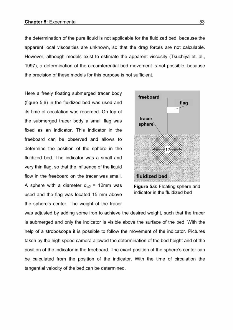
Chapter 5: Experimental 53
the determination of the pure liquid is not applicable for the fluidized bed, because the
apparent local viscosities are unknown, so that the drag forces are not calculable.
However, although models exist to estimate the apparent viscosity (Tsuchiya et. al.,
1997), a determination of the circumferential bed movement is not possible, because
the precision of these models for this purpose is not sufficient.
Here a freely floating submerged tracer body
(figure 5.6) in the fluidized bed was used and
its time of circulation was recorded. On top of
the submerged tracer body a small flag was
fixed as an indicator. This indicator in the
freeboard can be observed and allows to
determine the position of the sphere in the
fluidized bed. The indicator was a small and
very thin flag, so that the influence of the liquid
flow in the freeboard on the tracer was small.
A sphere with a diameter dts3 = 12mm was
used and the flag was located 15 mm above
the sphere’s center. The weight of the tracer
was adjusted by adding some iron to achieve the desired weight, such that the tracer
is submerged and only the indicator is visible above the surface of the bed. With the
help of a stroboscope it is possible to follow the movement of the indicator. Pictures
taken by the high speed camera allowed the determination of the bed height and of the
position of the indicator in the freeboard. The exact position of the sphere’s center can
be calculated from the position of the indicator. With the time of circulation the
tangential velocity of the bed can be determined.
Fahne
Freeboard
Wirbelschichtfluidized bed
flagfreeboard
tracer sphere
Figure 5.6: Floating sphere and indicator in the fluidized bed
12

54 Chapter 5: Experimental
5.3 Optimization of the coarse discharge
The coarse discharge plays an important role for the performance of the classifier. The
operation of the needle valves with the elbow lever was found to cause severe
disturbances to the classification process. For a high separation efficiency and a stable
cut size a constant bed height during operation is essential. It is also important, that
the coarse discharge is always submerged in the fluidized bed to avoid bypassing of
fines into the coarse fraction. The four needle valves operated by an elbow lever
mechanism have the drawback that the adjustment of the coarse suspension flow is
not sufficiently precise. To control the bed height, the bed is observed by a
stroboscope through the vision panels. As long as the bed height is below a certain
level the needle valves remain closed. When the bed height becomes too high, the
valves are opened. When the needle valves are open, a high volume flow leaving the
classifier at the coarse discharge can be observed. The coarse discharge volume flow
reduces significantly the radial flow of the classification water above the coarse
discharge, i.e. the cut size changes, while the coarse discharge is open.
Experiments showed also that the opening of the 4 needle valves results in a flushing
out of the bed material in a short time, such that the bed height was very fast reduced
to the height of the coarse outlet. In that case fines were misclassified into the coarse
fraction due to bypassing. In order to achieve a better separation performance a
constant flow rate of the coarse drain and a constant bed height above the coarse
discharge is necessary. The key to achieve these conditions is a modification of the
coarse discharge design. For that reason a coarse discharge based on an outlet
nozzle with constant aperture was introduced. The bed height in this system is self-
adjusting. An increase of the bed height increases the pressure at the nozzle, which
results in an increase of coarse suspension outflow, i.e. if the bed height is too high,
the solid off-take is increased and vice versa. At a certain bed height, an equilibrium is

Chapter 5: Experimental 55
reached and the outgoing flow and the bed height remain constant. Different types of
coarse discharges (figure 5.7) were tested and compared.
Figure 5.7: Types of coarse discharge mechanisms
The coarse discharge nozzle type II is a small pipe with a constant diameter of 1 mm,
installed at the side of the classification chamber 13.5 mm above the distributor. The
nozzle type III is quite similar to type II, but the difference is the tip of the type III
nozzle is located at the centre of the fluidized bed. The tip of the discharge nozzle type
IV is vertically oriented and facing the distributor at a height of 5 mm. In this case the

56 Chapter 5: Experimental
fines, which are supposed to be misclassified, have a longer tracking distance through
the fluidized bed, so that a reduction of misclassification can be expected.
5.4 The usage of the Richardson Zaki correlation for the prediction of the
expansion behavior
The intention to model the expansion behavior of the fluidized bed is the prediction of
the bed porosity depending on the operating conditions. The knowledge of allows
the calculation of the bed mass mB and the bed height HB with the help of the bed
pressure drop pB. The bed mass and the bed height are important parameters for the
operation of the classifier, which have to be controlled in industrial classification
processes. The control of the bed height for a given throughput can be achieved by a
partial recirculation of the coarse fraction to enhance the feed mass flow in case of a
too low bed height. The control of the bed height by recirculation is not part of the
present work, but might be of interest for later industrial applications. For the present
work the bed height is a parameter which is important to be determined for the
investigation of its influence. In the classification process at high feed rates it is
impossible to determine the bed surface directly due to turbidity, so that the bed
pressure drop is the only usable information. To model the coarse discharge the
knowledge of the bed porosity is also of importance, because the pressure drop over
the discharge nozzle is depending on both, the bed height and the porosity.
In the fluidized state the bed is completely supported by the liquid, an increase of the
fluidizing velocity results in an increase of the bed porosity at a constant bed
pressure drop in the gravity field. In the centrifugal field the centrifugal acceleration
changes with the radius, whereby the pressure drop decreases during expansion due
to a radial shift of the mass center. Different approaches have been proposed in
literature to model the expansion behavior of the bed (G. Bickert, 1997; N. Hidaka et
al., 1994). One of the simplest and most handy approaches is the one by Richardson
Chapter 5: Experimental 57
and Zaki (J.F. Richardson, W.N. Zaki, 1954). They investigated the swarm settling of
monodisperse spheres and found the following power law, which nowadays is also
widely used to describe the expansion behavior of liquid fluidized beds:
u/ut = n, (5.12)
where u is the swarm settling velocity and ut denotes the terminal velocity of a single
particle. If a fluidized bed is described u stands for the superficial fluidizing velocity.
The Richardson Zaki exponent n is depending on the particle Reynolds number Rep:
p
p
p
p
p
p
p
p
p
p
p
p
(5.13)
where Rep is defined by:
Rep = ut * dp * -1 (5.14)
The terminal settling velocity ut is related to the particle diameter dp and is in the
centrifugal field calculated from
p 2s L
tL D s
d4u * * * 1 * r *
3 c
r r wr r
æ ö÷ç ÷= -ç ÷ç ÷çè ø (5.15)
In the present work the settling velocity of the mean particle diameter dp,50 is used to
characterize the size distribution of the fluidized particles. As particle Re-numbers for
the dp,50 exceed the validity limits for the Stokes law (Re > 0.25) at higher angular
velocities, the KASKAS drag model (Stieß, 1993):
Dp p
24 4c 0
Re Re= + + .4 (5.16)

58 Chapter 5: Experimental
has been used for calculations of ut. The correlation by Kaskas is valid for Reynolds
numbers Rep < 2*105.
An explicit expression for the terminal velocity is not possible, because of the
dependence of the drag coefficient on the terminal velocity and vice versa. The
terminal velocities were therefore calculated by a MATLAB iteration and can be taken
from the diagram in figure 5.8 for different operating conditions. Figure 5.9 shows the
corresponding Reynolds numbers.
Although the terminal velocity ut and the radial velocity u are depending on the radius
in a rotating system, the ratio u/ut turns out to be nearly constant due to the special
shape of the classification chamber. This is illustrated in the example shown in figure
5.10. For a fluidizing throughput of 1 m3/h, which is equivalent to 0.005 m/s fluidizing
velocity, the ratio of u/ut is plotted over the radius of the classification chamber. It can
be seen that the deviations of the radius-depending ratios u(r)/ut(r) from the ratio
u(RD)/ut(RD) at the distributor are very small and can therefore be neglected. In the
following the term u/ut is always related to the radius of the distributor.
To apply the Richardson Zaki model on the bed expansion behavior of the classifier
the porosity must be determined experimentally and correlated with u/ut. If the
condition
d(log u/ut)/d(log ) = const. (5.17)
is fulfilled the Richardson Zaki correlation is valid. The Richardson Zaki exponent n
can then be determined by plotting log(u/ut) versus log(). The slope of a straight line
through the plotted values is the Richardson Zaki exponent n. The porosity can be
calculated from
S
B s
m1
V
, (5.18)

Chapter 5: Experimental 59
Figure 5.8: Terminal velocities for particles at the distributor radius (RD = 0.445 m) with a density of 2650 kg/m3 settling in the centrifugal classifier operated with water at 10°C ( = 1300 kg /m s)
Figure 5.9: Reynolds numbers for particles at the distributor radius (RD = 0.445 m) with a density of 2650 kg/m3 settling in the centrifugal classifier operated with water at 10°C ( = 1300 kg /m s)
0.00
0.05
0.10
0.15
0.20
0.25
0 10 20 30 40 50 60
particle size [m]
term
inal
vel
oci
ty [
m/s
]
300 rpm400 rpm500 rpm600 rpm
0.0
0.5
1.0
1.5
2.0
2.5
3.0
3.5
4.0
4.5
5.0
0 10 20 30 40 50 60
particle size [m]
par
ticl
e R
eyn
old
s n
um
ber
[-]
300 U/min Re-kaskas400 U/min Re-kaskas500 U/min Re-kaskas600 U/min Re-kaskas

60 Chapter 5: Experimental
if solids mass of the fluidized bed mS, solids density S and bed volume VB are known.
The bed mass mS is determined by balancing all of the incoming and outgoing flows
and concentrations during the build-up of the bed. By taking pictures of the bed with
the high speed camera through the observation window the bed height HB was
measured and then the bed volume VB was calculated. It is has to be mentioned that
is the average porosity of the fluidized bed, possible porosity gradients are not
considered in this work.
Figure 5.10: Fluidizing to terminal velocity ratios for a 30 m particle over the radius of the classification chamber for a fluidizing water throughput of 1m3/h
0.00
0.05
0.10
0.15
0.20
0.25
0.30
0.335 0.357 0.379 0.401 0.423 0.445radial position [m]
u/u
t [-
]
300 rpm400 rpm
500 rpm
600 rpm
weir distributor
For the comparison of different bed materials at different centrifugal accelerations, it is
important to investigate fluidized beds with similar particle size distributions. Therefore
the same procedure was always carried out for building up the fluidizing bed: a
number of revolution of 300 rpm was adjusted with a fluidizing velocity of 0.005 m/s.
Then 0.2 m3/h feed suspension with 4 vol-% solids content was introduced into the
classification chamber until the desired bed height was reached. During the built up

Chapter 5: Experimental 61
classification took place, whereby particles smaller than the cut size were elutriated
and the particle size distribution of the bed became significantly coarser than the one
of the original material. As the densities of the investigated materials were almost the
same (quartz sand: Q = 2650 kg/m3; glass: G = 2500 kg/m3; limestone: Li=2620
kg/m3) similar particle size distributions were achieved.
5.5 Measurement of the bed pressure drop
The proper characterization of the hydrodynamics is an important aspect in the wet
fluidization technology. The major interest in fluidized bed classification technology is
the minimum superficial velocity at which the bed is stably and completely fluidized.
Stability means that the bed is homogeneous and free from defluidized zones.
Instabilities can be observed through the vision panel as shown in figure 5.11 on its left
side. At the fluidized bed surface erupting voids are observed and the fluidized bed
surface is uneven. Possible reasons are insufficient distributor pressure drop, or the
existence of a wide particle size distribution, for which the radial velocity is not high
enough to achieve complete fluidization. Contrary, on the right hand side of figure 5.11
no eruptions of voids are visible and the bed surface is even, so that this bed can be
considered to be a stable, completely fluidized bed. The slightly concave shape of the
bed surface in figure 5.11 is caused by the curvature of the classification chamber.
When the fluid velocity for a polydisperse fixed bed of a wide size distribution is
increased the smaller particles are apt to slip into the voids between the larger
particles and are fluidized while the larger remain stationary. This partial fluidization
behavior causes the well-known smooth transition between fixed and fluidized bed
pressure drop. The classifier should be operated beyond this transition regime to
achieve a completely fluidized bed. On the other hand a too high fluidizing velocity via
the effect of the Coriolis force causes a strong tangential flow, which will induce
turbulence, what is certainly not favourable for the classification. Therefore a velocity

62 Chapter 5: Experimental
range has to be found, which is optimal for classification. For the purpose of finding the
optimum fluidization velocity a measurement of the pressure drop characteristics in the
centrifugal field is necessary.
Figure 5.11: Fluidized bed with instabilities (left) and stable fluidized bed (right) at 400 rpm
distributor
fluidized bed
uneven bedsurface
void eruptingfrom bed
distributor
fluidized bed
even bed surface
ud = 1.8 mm/s ud = 3.0 mm/s
A standard technique of pressure drop measurement in fluidization technology is the
liquid column gauge. Liquid column gauges consist of a vertical column of liquid in a
tube whose ends are exposed to different pressures. The column will rise or fall until
its weight is in equilibrium with the pressure differential between the two ends of the
tube. A very simple version is the U-tube (figure 5.12 left). One side is connected to
the region of interest while the reference pressure (which might be the atmospheric
pressure or a vacuum) is applied to the other. The difference in liquid level represents
the applied pressure. The pressure p exerted by a column of liquid of height h and
density ρL is given by the hydrostatic pressure equation,
p = h . g . ρL (5.19)
Therefore the pressure difference between the applied pressure pa and the reference
pressure po in a U-tube manometer can be found by solving

Chapter 5: Experimental 63
pa − po = h . g . ρL. (5.20)
The U-tube cannot directly be used in the rotating classifier, because it cannot be
assured that no water losses occur during startup and shutdown of the rotor. Therefore
a modified approach is considered. A single transparent tube is installed below the
distributor (figure 5.12 – right), which can be observed by the stroboscope or high
speed camera during operation. In the water filled classification chamber the water
column in the tube is levelled to the radial position of the weir, when no additional
water is introduced. If the water flow is turned on, the distributor pressure drop pD is
indicated by the rise of the water column in the transparent tube by rD.
The flow through the distributor with the area AD can be treated as a laminar flow
with a linear pressure drop characteristic.
V

64 Chapter 5: Experimental
D DD
V p = K A (5.21)
The constant KD can be determined by varying the volume flow in the solids free
chamber and measuring pD by taking photographs of the water column with the high
speed camera. The principle is illustrated by the photographs in figure 5.13.
V
Figure 5.13: Photograph of the transparent tube on the classifier and highspeed picture of the water filled transparent tube during operation
5.6 A concept of the control of the operation of the classifier
In order to achieve a stationary operation the coarse offtake was equipped with a
discharge nozzle. As has been shown above the flow through this nozzle is self-
adjusting within certain limits. However, in order to avoid overloading of the apparatus
it is necessary to always keep the bed level in a position between the overflow weir

Chapter 5: Experimental 65
and the opening of the coarse discharge nozzle. Monitoring the bed height is therefore
necessary for a control of the fluidized bed classifier.
The bed height can be observed through the windows by stroboscope lighting.
However, this is not possible under all operating conditions. For wide particle size
distributions in the classifier feed the boundary between the bed surface and the
freeboard is often difficult to distinguish. However, a measurement of the pressure
drop via the liquid column gauge is comparatively easy. Unfortunately, the relationship
between the bed height and the measured pressure drop is not straightforward.
Therefore, in the following the pressure drop of the distributor, fixed bed and fluidized
bed in the centrifugal field will be discussed in detail.
5.6.1 Calculation of the fluidized bed pressure drop from the liquid column
gauge
In the absence of a fluidized bed the indicated pressure drop pi of the liquid column
gauge equals the distributor pressure drop pD.
pi = pD (5.22)
In the presence of a fluidized bed the indicated excess height r of the water column is
changed due to the additional bed pressure drop
pi = pD + pB (5.23)
For the calculation of the bed pressure drop the distributor pressure drop has to be
subtracted from the indicated pressure drop pi:
pB = pi – pD (5.24)

66 Chapter 5: Experimental
The pressure drop for a fluidized bed in the gravitational field is:
pB = (s – L) . (1 – ) . g . HB (5.25)
where HB denotes the fluidized bed height. For the differential bed pressure drop in the
rotating fluidized bed it holds
dp/dr = (s – L) . (1 – ) . r . 2 (5.26)
from which it follows after integration
pB = 0.5 . (s – L) . (1 – ) . 2 . [RD
2 – RB2] (5.27)
which relates the radius of the bed surface RB to the bed pressure drop pB.
Conducting pressure drop measurements in the absence of a fluidized bed allows the
determination of the distributor pressure drop coefficient KD. In analogy to equations
(5.26) and (5.27) it holds for the indicated pressure drop pi:
pi = 0.5 . L . 2 . [RW
2 – (RW – r)2] (5.28)
Inserting equations (5.28),(5.21) and (5.27) into (5.24) yields
0.5 . (s – L) . (1 – ) . 2 . [RD
2 – RB2] = 0.5 . L
. 2 . [RW2 – (RW – r)2] – KD
. /AD V
(5.29)
Equation (5.29) provides a relationship between the radius of the fluidized bed surface
RB and the excess height r of the liquid column, which can now be used to calculate
the bed height HB from the indication of the liquid column gauge. The bed height is
given by:
HB = RD – RB (5.30)

Chapter 5: Experimental 67
5.6.2 Bed pressure drop model
Knowing the bed expansion behavior of the fluidized bed, the pressure drop can be
modelled when the bed mass and the operation parameters are known. The bed
expansion behaviour is expressed by a Richardson-Zaki type relationship as defined
by equation (5.12).
The pressure drop of the fluidized bed is
pB = 0.5 . (s – L) . (1 – ) . (RD
2 – RB2) . 2 (5.31),
where RD is radius of the distributor and RB the radius of the bed surface.
A differential volume element dV of the bed is described by:
dV = 2 . . B . r . dr; (5.32)
with the chamber width
B = K . r-2 (5.33)
and the chamber profile constant K = 0.00396 m3. Equation 5.33 is employed under
the assumption of a parabolic classification chamber profile as proposed by Schmidt.
The deviation of the realized two linear profiles (cf. figure 3.5) from the parabolic one
was proven (Schmidt, 2007) to be less than 2%, so that the use of (5.33) is justified.
The integration of (5.32) leads to the bed volume VB:
VB = 2 . . K . ln( RD/RB ) (5.34)
With
VB = mS / [s . (1 – )] (5.35)
the following expression for the bed surface radius RB can be derived:
SB D
s
mR R * exp
2 * * K * * (1 )p r eé ù-ê ú= ê ú-ë û
(5.36)

68 Chapter 5: Experimental
The usage of the Richardson - Zaki equation, (5.12) combined with (5.36) and (5.31)
results in
2 2 SnB s L D
nt s t
m1 up ( ) 1 R 1 exp
2 u K (1 u /u )r r w
p r
æ öé ùæ ö ÷-ç÷ç ê ú÷ç÷çD = ⋅ - ⋅ - ⋅ ⋅ ⋅ - ÷÷ ç ê úç ÷÷ ç÷ç ÷⋅ ⋅ ⋅ - ÷çè ø ê úè øë û (5.37)
With equation (5.37) the bed pressure drop in the fluidized state is related to the solids
mass in the fluidized bed mass. If the bed pressure drop was measured, equation
(5.31) combined with the Richardson Zaki equation (5.12) can be used to calculate the
radius of the fluidized bed surface RB:
(5.38)
( )2 B
B D2
ns Lt
2 pR R
u1 ur r w
⋅D= - æ ö÷ç- ⋅ - ⋅÷ç ÷çè ø
For the case, that the radius of the bed surface RB is known, the solids mass of the
bed can be calculated by transforming equation (5.36) in combination with (5.12) in
DnS S
t B
Rum 2 K 1 ln
u Rp r
æ ö÷ç ÷ç= ⋅ ⋅ ⋅ ⋅ - ⋅÷ç ÷÷çè ø (5.39)
As shown in chapter 5.4 the ratio of u/ut is approximately constant over the whole
radius of the classification chamber, so that
D
t t
uuu u (R
D ) (5.40)
is valid, where ut(RD) denotes the terminal particle velocity at the location r = RD. ut(RD)
is related to the Sauter diameter dps of the coarse fraction, which was determined from
samples, which were analyzed by laser diffraction analysis.

Chapter 5: Experimental 69
5.6.3 Pressure drop model for rotating fixed beds
For a given rotational speed the classification water throughput is limited at the lower
end by the minimum fluidizing velocity umf. Below umf the bed is in the fixed bed state
and thus no classification is possible. The estimation of umf in advance is therefore
essential for the selection of the operation parameters such as the angular speed of
the rotor and the classifying water throughput. The minimum fluidizing velocity umf can
be determined by the intersection of the fixed bed and the fluidized pressure drop
profile.
For the description of the fixed bed pressure drop it holds for the presently considered
fine particle system (Stieß, 1993):
22FB
K V3FB
(1 )dpC S
dr
u , (5.41)
Equation 5.41 is the Carman and Kozeny equation in its differential form. SV is the
specific surface of the particles, CK is the Kozeny coefficient and FB denotes the fixed
bed porosity. The Carman-Kozeny equation is valid for pure laminar flow for Rep < 3
(Stieß, 1993). For glass beads in water the particle Reynolds number Rep = 3 is
reached at 600 rpm for a Sauter diameter of 35 m. The Sauter diameters of the
particle beds in the present work were always below that value, so that the Carman-
Kozeny equation can assumed to be valid. The relationship between the specific
surface SV and the Sauter diameter for spheres is:
SV = 6 / dps (5.42)
In equation (5.41) the dependence of the flow velocity u on the radius r due to the
chamber profile has to be taken into account. It holds
D
D
uu
R r (5.43)

70 Chapter 5: Experimental
It follows
22FB D
K V3FB D
(1 ) u rdpC S
dr R
(5.44)
and after integration
FB
2 22 FB D FB
FB V K D3D
(1 ) R Rp 0.5 S C u
R
2
)
(5.45)
Equation (5.45) describes the pressure drop of the flow through the rotating fixed bed.
For the Kozeny constant a value of CK = 4 was used as proposed in literature (Stieß,
1993). The radial position of the fixed bed surface RFB can be calculated with equation
(5.36), when the fixed bed porosity FB and the solids mass of the bed mS are known.
The minimum fluidizing velocity can now be determined from the intersection of the
fixed bed pressure drop pFB(uD) with the fluidized bed pressure drop pB from
equation (5.37) for = FB. The fixed bed porosities were experimentally determined
for various conditions and can be found in chapter 6.
5.6.4 Determination of the operational parameters
In this chapter the operational parameters according to the separation task are
discussed. A separation task is normally defined by the solids feed mass flow M and
the desired cut size dC. The resulting solids flow of the coarse fraction through the
discharge nozzle is then given by:
S
CM
C S 3 CM M (1 Q (d ) (5.46)

Chapter 5: Experimental 71
The key parameters for designing the classification process in the present case with
regard to the cut size dC and solids throughput are the bed height, the angular velocity
and the coarse suspension mass flow . The coarse suspension mass flow
is defined as the sum of the solids mass flow and the water mass flow C
through the coarse discharge nozzle. The bed height can be chosen according to the
findings discussed in chapter 6. An adequate angular velocity has to be selected
corresponding to the cut size. Schmidt (2004) found that a higher angular speed of the
rotor results in a higher classification sharpness, so choosing a high angular speed is
recommendable for the achievement of a high classification performance. On the other
hand more water is consumed due to a higher demand of classification water
throughput and the cut size is deviating more from the theoretical one in direction to
larger particle sizes (Schmidt, 2004). Rotational speeds between 400 and 800 rpm are
recommended for cut sizes between 3 and 20 m for a particle density of 2650 kg/m3
in water.
SUS,CM
SUS,CM CM
For a specified classification task the coarse suspension mass flow through the
discharge nozzle is the parameter, which has to be adapted. This can be
obtained by selecting an appropriate discharge nozzle with the required orifice
diameter, which determines the throughflow. Therefore a model was developed to
calculate the flow through the nozzle depending on the radius of the bed
surface RB, on the angular velocity and on the nozzle diameter dN. In this model a
nozzle friction coefficient was introduced, which was determined for the nozzles of
the present work by the experiments presented in chapter 6.
SUS,CM
SUS,CM
In the present work, where discharge nozzles, each with an orifice diameter of 1mm,
were used, the suspension mass flow through the nozzle is specified by the orifice
diameter for the operating point to be investigated. Therefore the model can be used
to estimate the permissible suspension feed flow corresponding to the operating

72 Chapter 5: Experimental
parameters and the nozzle orifice. Furthermore the model can be employed to
compare the measured coarse discharge with the theoretical one to detect bypasses
from the freeboard directly to the coarse recovery. In that case the bypass is indicated,
when the measured coarse discharge flow is significantly below the theoretical one.
The hydrostatic pressure increase dp over a ring element dr is defined as:
2L Sdp (1 ) r dr , (5.47)
With the mean fluidized bed density m:
m = L + (1 – ) . S (5.48)
it follows:
2mdp r dr (5.49)
The pressure drop of the nozzle pN is defined as the difference of the hydrostatic
pressure at the radial position of the nozzle inside the chamber and the ambient
pressure. The nozzle pressure drop pN can be calculated by integration of equation
(5.49) in the radial intervals of freeboard and fluidized bed:
pN = 0.5 . m . (RN2 – RB
2) 2 + 0.5 . L . (RB2 – RW
2) . 2 (5.50)
RN, RW and RB, are the radial positions of the coarse discharge, the weir and the
fluidized bed surface, respectively.
The pressure drop of a nozzle is defined (Bohl, 1991) for a single phase flow:
pN = 0.5 . L . . vN
2 (5.51)
with vN being the fluid velocity in the nozzle and denoting the nozzle pressure drop
coefficient. For a liquid-solid suspension with dp << dN a similar relationship to hold
pN = 0.5 . m . . vN2 (5.52)

Chapter 5: Experimental 73
is assumed, where L is replaced by the mean density m. The suspension velocity in
the nozzle (diameter dN) can be expressed by the suspension massflow through
the nozzle:
SUS,CM
2SUS,C N N mM d v
4
(5.53)
or with regard to vN:
SUS,CN 2
N m
4 Mv
d
(5.54)
Equating equations (5.52) and (5.50) and inserting (5.54) gives the suspension mass
flow through the nozzle:
2 2 2 22m N B L B W
SUS,C m N
(R R ) (R R )M d
4
(5.55)
The coarse mass flow is then
SC SUS,C
mM M (1 ) (5.56)
The porosity can be obtained from the Richardson – Zaki correlation after
rearranging it to the porosity :
n
t
u
u (5.57)
The experimentally determined values of the Richardson Zaki coefficient n are
presented in chapter 6.
For the Richardson Zaki correlation the required fluidizing velocity u and the average
particle settling velocity of the fluidized bed ut have to be estimated. The fluidizing

74 Chapter 5: Experimental
velocity u is correlated to the single particle settling velocity of the cut size dC at the
distributor:
2 2D s L CR ( ) d
u18
, (5.58)
which is valid in the Stokes range. The average particle diameter dp,50 of the fluidized
bed can obtained from the particle size distribution of the suspension feed under the
assumption of an ideal classification at the cut size dC. The corresponding terminal
velocity ut can then be taken from figure 5.8. By solving equation (5.55) with regard to
dN, a suitable nozzle diameter can be selected for the given classification task.
This model describes the outflow through the coarse discharge orifice under
completely turbulent conditions, i.e. the influence of the apparent suspension viscosity
is neglected. Furthermore a likely slip between liquid and particles is neglected.
Therefore the present model can only provide a rough estimation for choosing the
operating conditions. The pressure drop coefficient of the nozzle is determined
experimentally and can be found in chapter 6. Schmidt (2004) reported that the real
cut sizes are in the average overestimated in the range of a few microns. However this
approach can be used for choosing appropriate operating parameters.
To verify the feasibility of the classification task under the desired operating conditions,
the minimum fluidizing velocity of the bed material, i.e. the coarse fraction, has to be
estimated by equating the pressure drop models for the rotating fixed bed (equation
5.45) and fluidizing bed (equation 5.37), respectively. The particle size distribution of
the coarse fraction is given when an ideal classification at the cut size dc is assumed.
When the chosen fluidizing velocity uD is larger than the calculated minimum fluidizing
velocity the feasibility of the classification at that angular velocity is proven. In the final
chapter 6.10 a practical example of the above control strategy is provided.
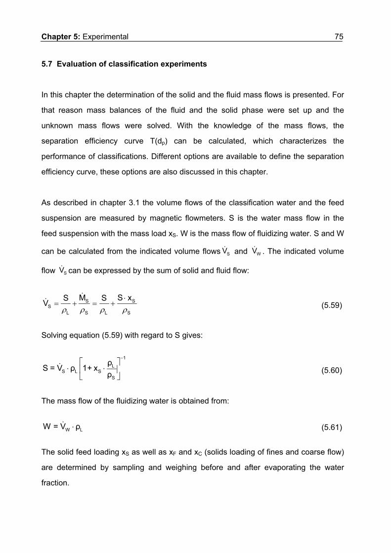
Chapter 5: Experimental 75
5.7 Evaluation of classification experiments
In this chapter the determination of the solid and the fluid mass flows is presented. For
that reason mass balances of the fluid and the solid phase were set up and the
unknown mass flows were solved. With the knowledge of the mass flows, the
separation efficiency curve T(dp) can be calculated, which characterizes the
performance of classifications. Different options are available to define the separation
efficiency curve, these options are also discussed in this chapter.
As described in chapter 3.1 the volume flows of the classification water and the feed
suspension are measured by magnetic flowmeters. S is the water mass flow in the
feed suspension with the mass load xS. W is the mass flow of fluidizing water. S and W
can be calculated from the indicated volume flows and . The indicated volume
flow can be expressed by the sum of solid and fluid flow:
SV WV
SV
SS
L S L S
M SS SV
Sx
(5.59)
Solving equation (5.59) with regard to S gives:
1
LS L S
S
ρS = V ρ 1+ x
ρ
(5.60)
The mass flow of the fluidizing water is obtained from:
W LW = V ρ (5.61)
The solid feed loading xS as well as xF and xC (solids loading of fines and coarse flow)
are determined by sampling and weighing before and after evaporating the water
fraction.

76 Chapter 5: Experimental
The water mass flows of the coarse’ and fines fraction (C and F) are determined by
balancing the water and the solids mass flows:
Water mass balance: (5.62), SL L
S
dmdm ρS W F C
dt dt ρ=- ⋅ = + - -
where mL and mS are the water and solids mass in the classification chamber,
respectively. Bed and water mass in the classification chamber are linked due to the
displacement of water when bed mass is added.
Solids mass balance: (5.63) SS F
dmS x F x C x
dt= ⋅ - ⋅ - ⋅ C
The change of the solids mass in the bed dmS/dt can be determined by evaluating the
bed pressure drop during the build-up of the bed. When a constant bed height is
achieved it holds dmS/dt = 0. This is the case for the classification experiments, where
the sampling is started when the desired bed height is reached.
Combining the solid mass balance (5.63) with the water mass balance (5.62), the
water mass flows of the fines and coarse, F and C, can be obtained:
Fines:
S LC C S
S
C F
dm ρ x 1 W x S (x xdt ρF
x x
æ ö÷ç⋅ ⋅ + + ⋅ - ⋅ -÷ç ÷çè ø=-
C )
(5.64)
Coarse:
S LF F S
S
F C
dm ρ x 1 W x S (x xdt ρC
x x
æ ö÷ç⋅ ⋅ + + ⋅ - ⋅ -÷ç ÷çè ø=-
F )
(5.65)

Chapter 5: Experimental 77
The mass fractions of coarse and fines are:
(5.66)
C
F C
C xc
F x C x
⋅=
⋅ + ⋅
(5.67),
F
F C
F xf
F x C x
⋅=
⋅ + ⋅
where c and f are the ratios of solid mass recovered in the coarse and fines fractions
to the solids mass in the feed. At a constant bed height, i.e. dmS/dt = 0, the coarse and
fines fraction can directly been calculated from the measured mass flows and solids
contents.
F S F C
F S F C C S C
[W x S (x x )] xc
[W x S (x x )] x [W x S (x x )] x
⋅ - ⋅ - ⋅=
⋅ - ⋅ - ⋅ - ⋅ - ⋅ - ⋅ F (5.68)
f = 1 – c (5.69)
The performance of the classification is characterized by the separation efficiency
curve T(dp). The separation efficiency is defined for a size class between dp and (dp +
ddp) as the ratio of the mass recovered in the coarse fraction to the mass initially
present in the feed. The separation efficiency can be calculated from different
measurements, because the dependence
S p C p F pq (d ) c q (d ) f q (d )= ⋅ + ⋅ (5.70)
allows different expressions for the definition of the separation efficiency curve, which
are presented below:
C pp
C p F p
c q (d )T(d )
c q (d ) f q (d )
⋅=
⋅ + ⋅ (5.71)

78 Chapter 5: Experimental
C pp
S p
c q (d )T(d )
q (d )
⋅=
(5.72)
F pp
S p
f q (d )T(d ) 1
q (d )
⋅= -
(5.73)
In the first case (equation 5.71), the separation efficiency curve is determined by
measuring the mass fraction of coarse’ and fines (c and f) and their density
distributions qC(dp) and qF(dp), respectively. The initially present particles of the feed
are expressed by the sum of particle masses recovered in the coarse and fines
fractions.
In the second case (equation 5.72) the mass fraction of the coarse recovery c and
their density distribution qC(dp) was measured and correlated with the density
distribution of the feed qS(dp).
In the third case (equation 5.73) the mass fraction of the fines recovery f and their
density distribution qF(dp) was measured and correlated with the density distribution of
the feed qS(dp).
Theoretically all three definitions should result into the same separation efficiency
curve. However errors occur in the measurement of the particle size distributions. This
results in a distortion of the separation efficiency curve, which can be expressed by an
error particle mass flow E (dp,i):
p,i S 3,S p,i 1 3,S p,i C 3,C p,i 1 3,C p,i
F 3,F p,i 1 3,F p,i
E(d ) S x [Q (d ) Q (d )] C x [Q (d ) Q (d )]
F x [Q (d ) Q (d )]
+ +
+
= ⋅ ⋅ - - ⋅ ⋅ -
- ⋅ ⋅ - (5.74)
If E(dp,i) <> 0, the mass balances of the interval (dp,i+1 – dp,i) are not fulfilled due to
errors in measurement or due to particle breakage and attrition. Even if a small
amount of particles are affected, especially for particle classes at the lower or higher

Chapter 5: Experimental 79
boundaries, the separation efficiency curve can be changed significantly. A definition
has to be chosen which is most robust to disturbances caused by errors and particle
comminution.
Figure 5.14 shows the mass flows of each particle class for feed, coarse and fines as
well as the balance error “mass flow” of the classification experiment from 24th of April
2008 as an example. In general the mass flow error is quite small, but has a high
contribution in the classes at the lower and higher end. It should be discussed how this
error is affecting the separation efficiency curves depending on their definition.
Therefore the separation efficiency curves of the classification experiments from 24.th
of April 2008 are compared in figure 5.15. The definition of equation (5.73) shows a
huge error in the separation efficiency curve in the lower micron range, because the
curve exceeds the limits of validity by becoming negative. The separation efficiency
curve defined by equation (5.72) exceeds the limits of validity in the coarse range by
becoming large than one. These errors originate from the sources discussed above.
The separation efficiency curves using these definitions are very sensitive to errors in
the particle class balances. When using the definition of equation (5.71), however, the
separation efficiency curve stays in the limits between zero and one. The latter
definition shows a very robust behavior concerning errors in the particle class mass
balances. Hence this definition is used for the calculation of the separation efficiency
curves in this work.

80 Chapter 5: Experimental
Figure 5.14: Mass flows of the particle classes and error mass flow (classification 24th April 2008)
Figure 5.15: Separation efficiency curves with different definitions (classification 24th April 2008)
-100
0
100
200
300
400
500
1 10 100
particle size [m]
pa
rtic
le c
las
s m
as
sfl
ow
[m
g/s
]
feedfinescoarseerror in balance
-0.2
0.0
0.2
0.4
0.6
0.8
1.0
1.2
1.4
1 10 100
particle size [m]
T [
-]
T(dp) c/(f+c)
T(dp) c/s
T(dp) 1-f/s
Chapter 5: Experimental 81
Besides the separation efficiency curve the sharpness defined by Eder (Stieß, 1993) is
a common definition for the characterization of the classification performance. The
sharpness is defined as the ratio of the particle sizes dp,25 and dp,75, where the
separation efficiency curves reaches 25% and 75% respectively:
= dp,25/ dp,75 (5.75)
Rumpf (Stieß, 1993) characterizes analytical sharp separations in the range between
0.9 < < 0.8, technically sharp separations between 0.8 < < 0.6 and usual technical
separations between 0.3 < < 0.6. The drawback of that definition is the fact, that
fishhook effects and local minima are not considered. For a more detailed
characterization the separation efficiency curve has to be considered.

06 Results and discussion
6.1 Fluid mechanics of the flow in the classification chamber
6.1.1 Results of the simplified model
The pure liquid flow in the classification chamber is calculated as described in chapter
4. The reason of the investigation is the generation of a tangential flow by the Coriolis
force, which turned out to have a strong influence on the flow pattern. For a rough
estimation a simplified model was used. In this model the observer is located outside
the system, so the absolute velocities are considered.
Equating the conservation of angular momentum with the wall friction results in a
tangential velocity profile. The profile is calculated with MATLAB iterating the
equations (4.16) to (4.18) over the chamber profile with a step width of r = - 0.0001
m. Calculations of the tangential velocity of the pure fluid have been done with the
simplified model with radial velocities at the distributor of 5.0 and 6.5 mm/s and
rotational speeds of 300, 400 and 600 rpm, respectively. The fluidization velocities
were chosen to be significantly higher than the minimum fluidization velocities in order
to allow a stable operation of the fluidized bed during the experiments, which were
carried out with the same velocities.
To check the influence of density and viscosity on the fluid mechanics, additional
calculations with air as fluid have been carried out with the same velocities and
rotational speeds. The wall friction coefficients are depending on the turbulence and
the Reynolds number of the flow, respectively. For Reynolds numbers Re > 2300 the
wall friction coefficient was set to 0.055, for Re < 1000 it was set to
= 96/Re (6.1)
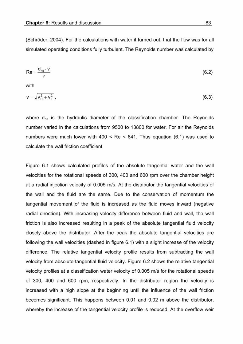
Chapter 6: Results and discussion 83
(Schröder, 2004). For the calculations with water it turned out, that the flow was for all
simulated operating conditions fully turbulent. The Reynolds number was calculated by
vd
Re hc (6.2)
with
2T
2R vvv , (6.3)
where dhc is the hydraulic diameter of the classification chamber. The Reynolds
number varied in the calculations from 9500 to 13800 for water. For air the Reynolds
numbers were much lower with 400 < Re < 841. Thus equation (6.1) was used to
calculate the wall friction coefficient.
Figure 6.1 shows calculated profiles of the absolute tangential water and the wall
velocities for the rotational speeds of 300, 400 and 600 rpm over the chamber height
at a radial injection velocity of 0.005 m/s. At the distributor the tangential velocities of
the wall and the fluid are the same. Due to the conservation of momentum the
tangential movement of the fluid is increased as the fluid moves inward (negative
radial direction). With increasing velocity difference between fluid and wall, the wall
friction is also increased resulting in a peak of the absolute tangential fluid velocity
closely above the distributor. After the peak the absolute tangential velocities are
following the wall velocities (dashed in figure 6.1) with a slight increase of the velocity
difference. The relative tangential velocity profile results from subtracting the wall
velocity from absolute tangential fluid velocity. Figure 6.2 shows the relative tangential
velocity profiles at a classification water velocity of 0.005 m/s for the rotational speeds
of 300, 400 and 600 rpm, respectively. In the distributor region the velocity is
increased with a high slope at the beginning until the influence of the wall friction
becomes significant. This happens between 0.01 and 0.02 m above the distributor,
whereby the increase of the tangential velocity profile is reduced. At the overflow weir

84 Chapter 6: Results and discussion
Figure 6.1: Absolute tangential velocities calculated with the simplified model for
different rotational speeds and a constant fluidizing velocity of 5 mm/s at the distributor
Figure 6.2: Relative tangential velocity profiles calculated from the simplified model at
different rotational speeds at a constant fluidizing velocity of 5 mm/s at the distributor
0
5
10
15
20
25
30
0.00 0.02 0.04 0.06 0.08 0.10height above the distributor [m]
ab
so
lute
ta
ng
en
tia
l v
elo
cit
y [
m/s
]
abs. fluid velocity at 300 rpmwall velocity at 300 rpmabs. fluid velocity at 400 rpmwall velocity at 400 rpmabs. fluid velocity at 600 rpmwall velocity at 600 U/min
distributor overflow weir
0.0
0.2
0.4
0.6
0.8
1.0
1.2
1.4
0.00 0.02 0.04 0.06 0.08 0.10height above the distributor [m]
rela
tiv
e t
an
ge
nti
al v
elo
cit
y [
m/s
]
rel. fluid velocity at 300 rpm
rel. fluid velocity at 400 rpm
rel. fluid velocity at 600 rpm
distributor overflow weir

Chapter 6: Results and discussion 85
at 0.11 m above the distributor relative tangential velocities of about 0.8 m/s (300 rpm),
0.9 m/s (400 rpm) and 1.1 m/s (600 rpm) were reached. The tangential velocity profile
was also calculated for water and air with a radial flow velocity of uD = 0.0065 m/s at
the distributor. The result is pictured in figure 6.3. The transition of the water velocity
profile from a steep to a slight slope is much smoother than in the case of uD = 0.005
m/s. Also the tangential velocities of 0.85 m/s and 0.35 m/s for 300 rpm and 600 rpm
at the overflow weir are much higher than in the case of 0.005 m/s.
Figure 6.3: Profiles of the relative tangential velocities calculated from the simplified
model for water and air at a constant fluidizing velocity of 6.5 mm/s at the distributor
0.0
0.2
0.4
0.6
0.8
1.0
1.2
1.4
0.00 0.02 0.04 0.06 0.08 0.10height above the distributor [m]
rela
tiv
e t
an
ge
nti
al v
elo
cit
y [
m/s
]
rel. air velocity at 300 rpmrel. water velocity at 300 rpmrel. air velocity at 600 rpmrel. water velocity at 600 rpm
distributor overflow weir
It can be seen from the calculation result that for both fluids the tangential velocity
component is two orders of magnitude higher than the radial one. Another result is the
increase of the tangential velocity with increasing rotational speed and also with
increasing radial velocities. For air the tangential velocity is much lower compared to
water for the same operating conditions. The reason is the change of the ratio of the

86 Chapter 6: Results and discussion
inertial force and the frictional forces due to the lower density and higher viscosity of
the gas.
6.1.2 Results of the CFD simulation
A more complicated but also more precise way to predict the flow pattern is the CFD
simulation. The advantage of the CFD simulation is that a 3 dimensional flow pattern is
provided and that all forces acting on the fluid are considered. High computing power
and long calculation times are required for an accurate calculation. A CFD calculation
can be applied to confirm the findings of the simplified model and to give a deeper
insight into the behavior of the flow. A vertical profile of the flow for a classification
velocity of uD = 0.005 m/s at a rotational speed of 300 rpm in the water-filled and
solids-free classification chamber calculated by the CFD-Simulation is shown in figure
6.4 a. The velocity vectors on a cut line through the chamber are mainly oriented in
tangential direction, the vertical component of the velocities can hardly be detected. In
figure 6.4 b it can be seen that the tangential velocity in the case of air is much lower
compared to water under the same conditions, although the Coriolis acceleration
ca 2ω u
(6.4)
is independent of density and viscosity. As explained before, the effect of friction,
which is much higher for air, causes the lower tangential velocities. The tangential flow
pattern itself can not directly be assessed as a negative effect on the classification
performance as long as the radial velocity component is undisturbed. However, it can
be expected that turbulence is induced in the freeboard influencing the radial velocity
profile. This influence may result in blurring the separation efficiency curve T(dp),
which does not occur in the normal gravity field.

Chapter 6: Results and discussion 87
overflow
porous distributorplate
b) aira) water
Figure 6.4: CFD-simulation of the pure fluid flow: (a) with water and (b) with air
(rotational speed: 300 rpm, radial velocity at distributor: 5.0 mm/s)
porous distributor plate
0 0.5 0.75 [m/s] rel. velocity
0 0.2 0.75 [m/s] rel. velocity
One could imagine that a segmentation of the classification chamber could suppress
the Coriolis-induced tangential flow. Therefore this case was investigated, too. Figure
6.5 shows the flow pattern on a cut surface of the classification chamber for a
completely closed classification chamber at the same conditions as for the
circumferential system (300 rpm; uD = 0.005 m/s). In this configuration much lower
tangential velocities occur than in the circumferential chamber. The velocity vectors
are not oriented radially, as it is desired for high separation efficiencies. On the
contrary, vortices are found caused by the presence of the Coriolis force, with vortex
velocities of one magnitude higher than the fluidizing velocity. It can be expected that
the occurrence of vortices decreases the classification performance significantly,
because vortices are affecting directly the radial velocity component, which is decisive

88 Chapter 6: Results and discussion
for classification. It can be expected that large particles are lifted inside vortices,
whereas very fine particles are transported downwards. Therefore coarse and fines
can be misclassified due to vortices. Such a configuration (which has been used by
Timmermann, 1998) is therefore not recommended for classification purposes.
no slipwall
no slipwall
direction of rotationinlet with radial fluid injection
opening for fluid outlet
Figure 6.5: CFD-simulation of the pure water flow in a closed chamber (rotational
speed: 300 rpm, radial velocity at distributor: 5.0 mm/s)

Chapter 6: Results and discussion 89
6.1.3 Comparison of the results of the simplified model with CFD calculations
and experiments conducted with a tracer sphere
To verify the theoretical results of the circumferential velocity profile, the tangential
velocities have been determined experimentally by the method described in section
5.2. The figures 6.6 and 6.7 show comparisons between calculation and
measurements. Water flows of 1.0 and 1.3 m3/h, respectively, corresponding to the
radial classification velocities of 5.0 and 6.5 mm/s were used.
It can be seen that the results of the CFD-simulation, the simplified model and the
experimental data are in good agreement. This provides evidence that both, the CFD-
simulation and the simplified model give reasonable results.
However in the distributor region some of the experimental results show larger values
than the calculated ones. An explanation lies in the fact, that for these measurements
the thread to the deflecting sphere is very short, which results in a reduced accuracy
for the velocity measurements. Also inhomogeneities in the flow through the distributor
may have an effect on the flow in the distributor region; such inhomogeneities will
dissipate with increasing distance to the distributor.

90 Chapter 6: Results and discussion
Figure 6.6: Comparison of the calculated tangential velocities (radial distributor
velocity of 5.0 mm/s) with experiments
Figure 6.7: Comparison of the calculated tangential velocities (radial distributor
velocity of 6.5 mm/s) with experiments
0.0
0.2
0.4
0.6
0.8
1.0
1.2
1.4
0.00 0.02 0.04 0.06 0.08 0.10
height above the distributor [m]
rela
tiv
e t
an
ge
nti
al v
elo
cit
y [
m/s
]
CFD simulation - 300 rpmCFD simulation - 400 rpmCFD simulation - 600 rpmsimplified model - 300 rpmsimplified model - 400 rpmsimplified model - 600 rpmexperimental - 300 rpmexperimental - 400 rpmexperimental - 600 rpm

Chapter 6: Results and discussion 91
6.1.4 The tangential velocity in the freeboard above the fluidized bed
The calculation of the tangential velocity in the freeboard above the fluidized bed was
carried out in the same way as in the case of pure liquid flow. The fluid above the
fluidized bed is assumed to be free of particles, i.e. the properties of the pure liquid
has been used for the calculation. For these investigations quartz was used.
The fluidized bed was always built up in such a way that the water filled classifier was
rotated at 300 rpm with 1 m3/h classification water. After the rotor had reached the
desired speed the suspension feed valve was opened and 0.2 m3/h suspension flow
(solids volume content 2%) was introduced. The accumulation of solids in the fluidized
bed was visually observed and the suspension feed was closed when the desired bed
height was reached. During the bed build up the fines were elutriated from the bed, so
that the particle size distribution differs from the raw material. This procedure ensures
that for all materials always a similar particle size distribution of the bed was achieved.
The median particle size was dp,50 = 30 m. For this test series only quartz was used
as bed material.
To measure the influence of a fluidized bed on the tangential velocity profile of the
freeboard the deflection of the tracer sphere was measured at a fixed radial position
37.5 mm above the distributor at a rotational speed of 300 rpm and at a water flow of
1 m3/h. Figure 6.8 shows as an example one picture of the sphere above the fluidized
bed. In this series of experiments the bed height was stepwise increased from 0 m to
0.031 m, i.e. the minimal distance of the bed surface to the bottom line of the sphere
was 1.5 mm. From the results (figure 6.9) it can be seen, that the tangential velocity is
approximately constant between 0.8 and 0.9 m/s with increasing bed height.

92 Chapter 6: Results and discussion
Figure 6.8: Photograph of the tracer sphere above the fluidized bed for the
determination of the tangential velocity in the freeboard (rotational speed: 300 rpm;
radial velocity at the distributor level: 5.0 mm/s)
rela
tive
ta
ng
enti
al v
elo
city
[m/s
]
location of the bottomside of the sphere
Figure 6.9: The tangential velocity in the freeboard measured with the tracer sphere
depending on the bed height (rotational speed: 300 rpm; radial velocity at the
distributor level: 5.0 mm/s)
location of the bottom side of the sphere

Chapter 6: Results and discussion 93
Only when the surface of the bed is approaching the bottom line of the sphere a slight
drop of the tangential velocity can be seen which is caused by the much slower
moving fluidized bed. At distances from the bed surface exceeding 5 mm the bed has
no influence on the tangential velocity, so that the values from the simulation of the
pure liquid flow are applicable to the freeboard.
6.1.5 Motion of the fluidized bed in the centrifugal field
To measure the influence of the Coriolis force on the fluidized bed itself, experiments
were carried out with the freely floating tracer sphere as described in section 5.2.2.
The measurements were done with radial velocities between 3 and 5 mm/s at 300 rpm
and 400 rpm. A picture of the almost completely submerged floating sphere in the bed
and its indicator is given in figure 6.10.
Figure 6.10: The freely floating sphere with the indicator in the fluidized bed
The figures 6.11 and 6.12 show the bed heights, the positions of the sphere in the bed
and the tangential velocities of the sphere plotted vs. the water flow for rotational
speeds of 300 and 400 rpm, respectively. For the lower rotational speed the sphere’s
position was always closely below the bed surface in the fluidized bed. It is assumed

94 Chapter 6: Results and discussion
that the sphere’s tangential velocity equals the one of the bed at this position. The bed
expands as the flow is increased. At the same time the sphere dips deeper into the
fluidized bed, which is due to the decreasing bed density with increasing expansion.
Furthermore an increase of the tangential velocity with increasing radial flow can be
observed, as it has been found also for the pure liquid. For the higher rotational speed
(400 rpm) the sphere again dips deeper into the bed at the beginning, but then it is
fully submerged and starts to change its position. The higher the radial velocity the
closer is the position of the sphere to the distributor. The fact, that the sphere does not
completely sink to the bottom as soon as it is fully submerged, indicates that there is a
vertical gradient of the porosity inside the bed with a higher porosity at the upper end
and an increased density at the bottom.
The change of the sphere’s position for water flows greater than 800 l/h is the reason
for the decrease of the tangential velocity with further increasing water flows. Since the
sphere has the tangential velocity of the bed at its current position, the decreasing
tangential velocity indicates, that there is a gradient of the tangential velocity with
lower velocities near the bottom. This is similar to the behavior of the pure flow, which
also showed lower tangential velocities closer to the distributor. Furthermore, also the
velocity increases with increasing water flow. Tangential velocities of the bed between
0.10 m/s and 0.25 m/s were measured.
Although the tangential velocity of the fluidized bed is much smaller than the tangential
velocity of the water in the freeboard, the influence of the Coriolis force can be
assessed to be significant on the fluidized bed. Thus the bed can be described as a
fluidized bed moving in the direction of rotation. The optimization of the coarse
discharge presented in chapter 5 is based on this finding.

Chapter 6: Results and discussion 95
Figure 6.11: The position of the swimming sphere in the bed and its tangential
velocity depending on the throughput at 300 rpm
Figure 6.12: The position of the swimming sphere in the bed and its tangential
velocity depending on the throughput at 400 rpm
0
1
2
3
4
5
6
600 700 800 900 1000
fluidizing water flow [l/h]
hei
gh
t ab
ove
dis
trib
uto
r [c
m]
0.00
0.05
0.10
0.15
0.20
0.25
0.30
VT
,sp
he
re [
m/s
]
Height of the fluidized bed
Position of the sphere
Tangential velocity of the sphere
300 rpm
0
1
2
3
4
5
6
600 700 800 900 1000
fluidizing water flow [l/h]
hei
gh
t ab
ove
dis
trib
uto
r [c
m]
0.00
0.02
0.04
0.06
0.08
0.10
0.12
0.14
0.16
VT, s
ph
ere
[m
/s]
Height of the fluidized bed
Position of the sphere
Tangential velocity of the sphere
400 rpm

96 Chapter 6: Results and discussion
6.2 Pressure drop
6.2.1 Pressure drop of the distributor
The pressure drop characteristics were measured as described in chapter 5 with a
liquid column in a transparent tube installed below the distributor. In this way the
distributor and the bed pressure drop are measured simultaneously. For the
determination of the bed pressure drop it is important to analyze the distributor
pressure drop characteristics first. A linear pressure drop profile with the slope KD (cf.
equation 5.21) is obtained and KD was measured before each experiment at different
angular velocities. Figure 6.13 shows the pressure drop profile of the distributor after
the installation of new distributor material at different angular speed rates. The profile
is linear and independent of the angular velocities. Porous distributor plates are known
to be sensitive to clogging (D. Kunii, O. Levenspiel, 1991). Figure 6.14 illustrates the
change of the pressure drop coefficient KD of the porous distributor plate after several
hours of operation.
The pressure drop coefficient increases significantly during long term operation. In
general high distributor pressure drops are known to increasing the fluidization stability
and therefore high bed pressure drop ratios are favored in fluidized bed applications
(D. Kunii, O. Levenspiel, 1991). Figure 6.15 illustrates the fluidization performance for
a new distributor and after 80 hours of operation at the same operating conditions. The
fluidized bed surface on the new distributor is very smooth, where on the right side
void eruptions and an uneven bed surface can be observed, i.e. the fluidization
performance is becoming worse. An explanation is that clogging occurs unevenly
distributed over the distributor. That results in a reduced fluidization down to a collapse
of the bed in some regions and to higher fluidizing velocities in other regions. The
classification performance is influenced by the fluidizing behavior and therefore the
distributor was exchanged after 80 hours of operation.

Chapter 6: Results and discussion 97
Figure 6.13: Pressure drop profile of a new porous distributor plate
0
5000
10000
15000
20000
25000
0.000 0.002 0.004 0.006 0.008 0.010fluidizing velocity uD [m/s]
dis
trib
uto
r p
res
su
re d
rop
[P
a] 300 rpm
400 rpm
500 rpm
Linear (400 rpm)
distributor pressure drop:
pD = KD . uD
-> KD = 2667424 [kg . m-2 . s-1]
Figure 6.14: Time dependency of the distributor pressure drop
0.0E+00
2.0E+06
4.0E+06
6.0E+06
8.0E+06
1.0E+07
1.2E+07
1.4E+07
0 10 20 30 40 50 60 70 80
time of operation [h]
pre
ssu
re d
rop
co
effi
cien
t K
D [
kg m
-2 s
-1]

98 Chapter 6: Results and discussion
6.2.2 The fluidized bed pressure drop
Knowing the distributor pressure drop characteristic the bed pressure drop profile can
be determined from the height of the liquid column using equation 5.24. The pressure
drop characteristics of glass beads, limestone and quartz were investigated. The
fluidized bed was build up with a sealed coarse discharge under a constant solids feed
rate of 200 l/h at 300 rpm. During the bed build up classification took place, i.e. a fines
fraction was elutriated from fluidized bed. Using always the same build-up procedure
assured that different raw materials with densities in the range between 2500 kg/m3
and 2650 kg/m3 have comparable particle size distributions in the fluidized bed. By
measuring the incoming and outgoing solids mass flows the solids mass of the bed
was calculated. The suspension feed and the fluidizing water were shut down when
the desired bed mass was reached. The sudden shutdown of the fluidizing water is
causing the bed to collapse immediately. Figure 6.16 shows the particle size
distribution of the bed materials glass beads, limestone and quartz. The median
diameters were dp,50,quartz = 31 m, dp,50,limestone = 30 m and dp,50,glass = 30 m. From
the fixed bed state the fluidizing water is stepwise increased until a fluidizing velocity of
0.005 m/s is reached and then decreased back to the fixed bed state. This procedure
was chosen to find out, if differences between the profiles of increasing and
decreasing fluidizing velocities occur.

Chapter 6: Results and discussion 99
Figure 6.16: Particle size distribution of the bed materials
0
25
50
75
100
1 10 100particle diameter [m]
cum
ula
tive
mas
s fr
acti
on
[%
]
limestoneglass beads
quartz
The pressure drop profile of glass beads fluidized at 400 rpm is pictured in figure 6.17.
With increasing fluidizing velocity an increase of the bed pressure drop can be
observed until a peak at approximately uD = 0.0016 m/s of pB = 15000 Pa is reached.
Beyond uD = 0.0016 m/s the pressure drop is decreased back to the static pressure
drop and stays constant between 12000 and 14000 Pa. A behavior like this has often
been described in the literature (e.g. Kunii & Levenspiel, 1991). Just right before the
onset of fluidization, the pressure drop reaches a maximum slightly higher than the
static bed pressure drop with a fixed bed porosity m slightly below the minimum
fluidizing porosity mf. A further increase of the distributor velocity causes the fixed bed
to unlock, i.e. particles are getting fluidized and the bed porosity is increased from m
to mf. As the porosity measurement in the rotating system is not precise enough to
distinguish between fixed bed porosity m and minimum fluidizing velocity mf, they are
treated as being the same.
With decreasing fluidizing velocity the bed volume is reduced until the particles form a
fixed bed with the porosity near mf. From the measurements a minimum fluidizing
velocity at the distributor level of 0.0016 m/s is obtained. The scatter of the measured

100 Chapter 6: Results and discussion
points indicates the limits of accuracy of the pressure drop measurement in the
rotating system.
The calculated fluidized bed pressure drop characteristic is indicating that the bed
pressure drop is slightly decreasing with increasing fluidizing velocity. This is contrary
to the situation in the gravitational field where the bed pressure drop is independent of
the fluidizing velocity. The explanation is, that in the rotating system with increasing
fluidizing water flow the bed is expanding. During expansion the center of gravity of the
bed will be displaced towards the axis of rotation where the centrifugal acceleration is
lower and therefore the “weight” of the bed is apparently reduced. However, this effect
is very small and hardly to be seen in figure 6.17.
The results for quartz with a solids mass in the fluidized bed of mS = 1.6 kg are
pictured in figure 6.18. A linear pressure drop characteristic can be observed in the
fixed bed state with distinct differences between increasing and decreasing water flow.
At approximately 0.0013 m/s the transition from the fixed to the fluidized bed takes
place. The transition from fixed to fluidized bed is much clearer in the case of quartz
compared to glass beads. The corresponding pressure drop is p = 12500 Pa at the
state of incipient fluidization. The fluidized bed pressure drop is quite in a good
agreement with the calculated pressure drop of approximately 13000 Pa.
To confirm the model for quartz, the theoretical profile was compared with
experimental data at a higher rotational speed of 500 rpm and a lower solids mass of
mS1kg (figure 6.19). Using a minimal fluidizing porosity of mf,quartz = 0.50 and a
minimal fluidizing velocity of umf = 0.0023 m/s, the pressure drop for incipient
fluidization was calculated from the intersection of the fixed and fluidized bed pressure
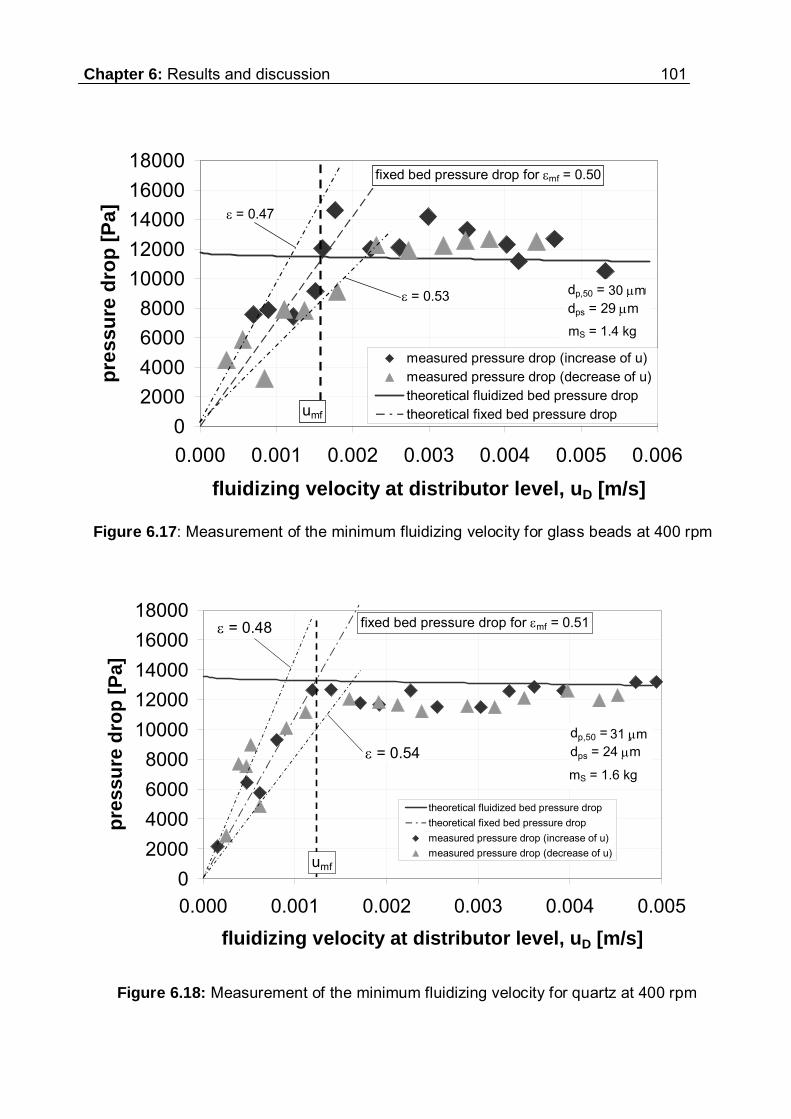
Chapter 6: Results and discussion 101
Figure 6.18: Measurement of the minimum fluidizing velocity for quartz at 400 rpm
Figure 6.17: Measurement of the minimum fluidizing velocity for glass beads at 400 rpm
0
2000
4000
6000
8000
10000
12000
14000
16000
18000
0.000 0.001 0.002 0.003 0.004 0.005 0.006
fluidizing velocity at distributor level, uD [m/s]
pre
ss
ure
dro
p [
Pa
]
fixed bed pressure drop for mf = 0.50
measured pressure drop (increase of u)measured pressure drop (decrease of u)theoretical fluidized bed pressure droptheoretical fixed bed pressure drop
dp,50 =dps = 29 m
31 m
mbed = 1.4 kg
umf
= 0.47
= 0.53 30 m
0
2000
4000
6000
8000
10000
12000
14000
16000
18000
0.000 0.001 0.002 0.003 0.004 0.005
fluidizing velocity at distributor level, uD [m/s]
pre
ssu
re d
rop
[P
a]
fixed bed pressure drop for mf = 0.51
theoretical fluidized bed pressure drop
theoretical fixed bed pressure drop
measured pressure drop (increase of u)
measured pressure drop (decrease of u)
dp,50 =dps = 24 m
28 m
mbed = 1.6 kg
umf
= 0.48
= 0.5431 m
mS = 1.4 kg
mS = 1.6 kg

102 Chapter 6: Results and discussion
drop curves. A fluidized bed pressure drop pbed = 13000 Pa was calculated, which is
in good agreement with the measured results.
Figure 6.19: Measurement of the minimum fluidizing velocity for quartz at 500 rpm
0
2000
4000
6000
8000
10000
12000
14000
16000
18000
0.000 0.001 0.002 0.003 0.004 0.005 0.006 0.007
fluidizing velocity at distributor level, uD [m/s]
pre
ssu
re d
rop
[P
a]
measured pressure drop
theoretical fluidized bed pressure drop
theoretical fixed bed pressure drop
dp,50 = 30 mdps = 25 mmbed = 1.0 kg
umf
fixed bed pressure drop for mf = 0.50
= 0.52
= 0.48
dp,50 = 31 m m
S
dps = 25 m = 1.0 kg
The investigation of limestone is pictured in figure 6.20. With increasing fluidizing
water flow a maximum in the bed pressure drop is located at approximately 0.0016
m/s with p = 15600 Pa. With further increase of the fluidizing velocity the pressure
drop is then reduced to a range between 12000 and 14000 Pa.
The measurement of the pressure drop profiles allows a determination of the minimum
fluidizing velocity at the intersection of fixed and the fluidized bed pressure drop lines.
At fluidizing velocities of above 1.5 x umf, no difference between increase and decrease
was observed, i.e. the bed is completely fluidized. It can therefore be concluded that,
in order to ensure homogeneous fluidization for classification, a fluidizing velocity of uD
exceeding 1.5 x umf is necessary. Increasing the fluidizing velocity further results in an
increase of the tangential velocity, which enhances unfavourable turbulence.

Chapter 6: Results and discussion 103
Figure 6.20: Measurement of the minimum fluidizing velocity for limestone at 400 rpm
0
2000
4000
6000
8000
10000
12000
14000
16000
18000
0.000 0.001 0.002 0.003 0.004 0.005
fluidizing velocity at distributor level, uD [m/s]
pre
ss
ure
dro
p [
Pa
]
measured pressure drop (increase of u)
measured pressure drop (decrease of u)
theoretical fluidized bed pressure drop
theoretical fixed bed pressure drop
dp,50 = 30 mdps = 26 mmbed = 1.52 kg
umf
fixed bed pressure drop for mf = 0.51
= 0.54
= 0.48
mS = 1.52 kg
6.3 The expansion behavior of the fluidized bed
The expansion behavior of fluidized beds of quartz, glass beads and limestone was
investigated. The build up of the bed was conducted in the same way as for the
pressure drop characterization, so that particle size distributions as shown in figure
6.16 were achieved. Experiments on the bed expansion behavior were carried out by
varying the angular speed and fluidization velocity. A Richardson Zaki type power law
is used for the description of the expansion behavior. For the determination of the
exponent n the porosity on the abscissa is plotted versus the ratio of fluidizing and
terminal velocity u/ut on the ordinate on a logarithmic grid. As the Richardon Zaki
exponent n varies outside the Stokes range, i.e. Rep > 0.2, which is the case for the

104 Chapter 6: Results and discussion
investigated fluidized beds, the plots with the Richardson Zaki exponents from
literature are depending on the angular velocities. In figures 6.21 – 6.23 the plots of
the Richardson Zaki correlation for the materials glass beads, limestone and quartz
are shown for rotational speeds of 300 and 600 rpm. The deviation of both plots are
hardly detectable, so that the description of the expansion behavior was conducted
with only one exponent for the range between 300 and 600 rpm. From the literature
exponents between 4.36 and 4.42 were calculated under gravitational acceleration for
the same range of Reynolds numbers (Richardson, Zaki, 1954).
Figure 6.21: Bed expansion behavior of fluidized glass beads
-2.0
0.0
-0.4 -0.3 -0.2 -0.1 0
[-]
u/u
t [-]
300 rpm400 rpm600 rpmline of best fit--
0.6 0.7 0.8 0.5
1.0 0.8 0.6
0.4
0.2
0.1 0.08 0.06
0.04
0.02
0.01
u/ut = 4.9
0.4
glass beads
G = 2500 kg/m3
dp,50 = 33 m
0.9 1.0
calculated with Richardson-Zaki formula from literature forRe = 0.6 (300 rpm) Re = 2.2 (600 rpm)
In figure 6.21 the expansion behavior of glass beads is presented. The expansion
behavior was investigated for the rotational speed rates of 300, 400 and 600 rpm. The
data points can easily be represented by a straight line with the slope n of 4.9. The
exponent is slightly higher than n obtained from literature, which is between 4.36 and
4.42.

Chapter 6: Results and discussion 105
Figure 6.22: Bed expansion behavior of fluidized quartz powder
-2.0
0.0
-0.4 -0.3 -0.2 -0.1 0
[-]
u/u
t [-]
300 rpm400 rpm600 rpmline of best fit--
0.6 0.7 0.8
1.0 0.8 0.6
0.4
0.2
0.1 0.08 0.06
0.04
0.02
0.01
u/ut = 4.5
0.4
quartz
Q = 2650 kg/m3
dp,50 = 29 m
0.5 0.9 1.0
calculated with Richardson-Zaki formula from literature forRe = 0.6 (300 rpm) Re = 2.2 (600 rpm)
Figure 6.22 shows the expansion behavior of quartz. Here also all data points can be
represented by a single straight line, indicating, that the usage of a common exponent
for the range between 300 and 600 rpm is valid. The exponent for quartz has a value
of n = 4.5. The expansion behavior of limestone is shown in figure 6.23. The exponent
for the rates between 300 and 600 rpm is 5.9 in this case.
The spherical glass beads which are expected to be closest to the literature values
have a slightly higher n value than in the literature, which means that for given u/ut
and therefore the bed expansion is higher in the centrifugal field than in the
gravitational one. This can be explained by the superimposed tangential movement of
the bed in the centrifugal field.

106 Chapter 6: Results and discussion
Figure 6.23: Bed expansion behavior of fluidized limestone
-2.0
0.0
-0.4 -0.3 -0.2 -0.1 0
[-]
u/u
t [-]
300 rpm400 rpm600 rpmline of best fit--
0.6 0.7 1.0 0.5
1.0 0.8 0.6
0.4
0.2
0.1 0.08 0.06
0.04
0.02
0.01
u/ut = 5.9
fixed bed
0.4
limestone
Li = 2620 kg/m3
dp,50 = 32 m
0.8 0.9
calculated with Richardson-Zaki formula from literature forRe = 0.6 (300 rpm) Re = 2.2 (600 rpm)
6.4 Analysis of the particle size distributions
For the characterization of the classification performance a proper analysis of the
particle size distributions is essential. For this purpose many sophisticated methods
are available in industry. The most easiest and cheapest method is screening, but
screens are only available for particle sizes down to 25 m. Another method is the
sedimentation technique, which can be performed either in the normal gravity or in a
centrifugal environment. While gravity sedimentation is not suitable for particle sizes
below 10 m due to too low settling velocity, the centrifugal sedimentation analysis
was tested for the experimental materials in the disc centrifuge of the CPS company
(CPS Instruments Europe, Oosterhout, The Netherlands). The analysis of the used
materials revealed that this method is only precise between 0.01 and 10 m. Large

Chapter 6: Results and discussion 107
particles are not detected, because of too high settling velocities in the centrifugal field,
whereby the sedimentation has to be assessed as a not suitable analysis method for
the purpose of this work.
The determination was therefore conducted by laser diffraction analysis. Light from a
laser is sent into a cloud of particles, which are suspended in a transparent liquid e.g.
distilled water. The particles scatter the light, smaller particles scattering the light at
larger angles than bigger ones. The scattered light can be measured by a series of
photodetectors placed at different angles. This is known as the diffraction pattern for
the sample. The diffraction pattern can be used to measure the size of the particles
using light scattering theory that was developed in the early 20th century by Mie. As
the instrument measures clouds of particles rather than individual ones, it is known as
an "ensemble" technique, with the advantage that at smaller sizes e.g. 10 microns, the
system is measuring millions of particles which gives some statistical significance to
the measured results.
As the Mie theory is very complex a large amount of computing power and the
knowledge of the refraction index are required to evaluate the particle size distribution.
Therefore a simplified model, also known as Fraunhofer approximation, is widely used
for the evaluation. As the Mie theory is valid for the whole spectrum of particle sizes,
the Fraunhofer approximation is found to be unreliable in the lower micron range
(Malvern, 2000), i.e. for particles < 10 m. Therefore the two laser diffraction analyzer
of the Institute of Solids Process Engineering and Particle Technology at Hamburg
University of Technology, namely the Beckman Coulter (LS13320c – Beckman Coulter
GmbH, Krefeld, Germany) and HELOS (Sympatec GmbH, Clausthal – Zellerfeld,
Germany) were tested concerning their accuracy in the particle size measurement.
The HELOS provides the Fraunhofer approximation only, while the Beckman Coulter
provides both.

108 Chapter 6: Results and discussion
To find the most accurate evaluation method, it is necessary to compare the particle
size distributions of the same sample with a method, where accuracy can be assured.
This method can be an optical evaluation of >1000 particles taken by SEM pictures of
the sample. For the evaluation the software SCANDIUM (Olympus Soft Imaging
Solutions GmbH, Münster, Germany) was applied. SCANDIUM detects each particle
on SEM pictures and calculates each diameter from the cut surface. The detection
enables the calculation of a number density distribution, which can be converted in a
mass density distribution. Picture 6.24 shows the detection of limestone particles with
SCANDIUM. Detecting some thousand of particles this way (approx. 10 pictures) gives
an adequate number of particles for a particle size distribution determination.
Figure 6.24: Limestone particles on a SEM picture (left) detected with the evaluation software SCANDIUM (right)
The comparison of the methods for a limestone sample in figure 6.25 revealed that the
Mie evaluation and the SCANDIUM detection are in a quite good agreement in the
range below 10 m. The deviation in the range above 25 m can be explained by the
fact that not enough particles can be taken into account in the coarse region. As the
Fraunhofer approximation is known to be inaccurate in the fines region it can be
concluded that the fines content indicated in figure 6.25 is overrated, i.e. the detected

Chapter 6: Results and discussion 109
particles do not exist. Previous measurements (Schmidt, 2004) were conducted with
HELOS and evaluated with the Fraunhofer approximation. A strong fishhook effect,
wherein the recovery of fine particles in the coarse fraction increases with decreasing
particle size, was observed by Schmidt. This effect can now be explained by
overrating the fines due to an evaluation error of the Fraunhofer approximation. On the
contrary the evaluation with the Mie theory turns out to be accurate as is demonstrated
by the optical evaluation.
0
10
20
30
40
50
60
70
80
90
100
1 10 100particle size [m]
Q3
[%
]
Beckman Coulter - Mie
SCANDIUM - SEM picture analysis
HELOS - Fraunhofer
Beckman Coulter - Fraunhofer
Figure 6.25: Limestone sample analyzed with different methods
To illustrate the effect of the evaluation error, the density distributions and the
separation efficiency curves of the classification experiment from the 23.th May 2008
evaluated with Mie theory and Fraunhofer approximation are presented in figure 6.26.
The top left diagram shows the density distributions of the suspension feed, the coarse
and the fines fractions. Submicron particles are really rare and are hardly to detect in
the fines fraction and the suspension feed. These findings were confirmed by the
SEM-analysis as described above. What happens when the Fraunhofer approximation

110 Chapter 6: Results and discussion
Figure 6.26: Mass density distributions before and after quartz classification and
separation efficiency curve evaluated with Mie theory and Fraunhofer approximation
(experiment 23th May 2008: 700 rpm; fluidizing velocity: 0.0031 m/s)
0
40
80
120
160
200
1 10 100
particle size [μm]
q3 [
%/μ
m]
density distributionfinescoarsesuspension feed
0
40
80
120
160
200
1 10
particle size [μm]
q100
3 [%
/μm
]
density distributionfinescoarsesuspension feed
Mie theory Fraunhoferapproximation
0
0.1
0.2
0.3
0.4
0.5
0.6
0.7
0.8
0.9
1
1 10 100
particle size [μm]
sep
ara
tion
eff
icie
ncy
[-]
Fraunhofer
Mie
is applied is shown on the picture at the top right. In the range below 1 m up to 10 m
the particle classes are increased by not existing particles, what has an significant
effect on the separation efficiency curve, especially in the regions at the upper or lower
end, where the total mass in the particle classes are small. A ‘detection’ of not existing
particles in the coarse fraction combined with a large coarse fraction c results in a

Chapter 6: Results and discussion 111
fishhook effect as shown at the bottom of figure 6.26. This fishhook effect is only
based on evaluation errors of the Fraunhofer approximation in the range below 10 m.
Thus the particle analysis in this work has been conducted with the Beckman Coulter
using the Mie theory only.
6.5 Classification experiments with the original configuration of solids discharge
Previous classification experiments were carried out with the elbow lever mechanism
for coarse withdrawal. As described above the elbow lever mechanism is not capable
to control the bed height accurately, which, however, is necessary for a sharp
classification. Another problem is the occurrence of a flushing out of the bed material,
what leads to misclassification due to bypass of fines to the outlet.
In the previous work (Schmidt, 2004) inaccurate separation efficiency curves were
found with a huge amount of fines being misclassified into the coarse fraction. Figure
6.27 is picturing separation efficiency curves of classification experiments at 400 rpm
by Schmidt, where the suspension feed to fluidizing water ratio was investigated.
Schmidt found that the lower the ratio the more efficient is the classification
performance. The water injected through the feed ports is only affecting particles
above the ports and is less homogeneous distributed compared to an injection through
the distributor, so that the better classification performance for a lower ratio can be
explained.
But even the separation efficiency curve with the lowest suspension feed-to-fluidizing
water ratio shows a very strong fishhook effect. On one hand the fishhook can be
explained by errors in the evaluation of the laser diffraction patterns with the
Fraunhofer model, resulting into an overrating of fines. On the other hand a reason
might be the use of the elbow lever mechanism for coarse discharge. For clarification

112 Chapter 6: Results and discussion
Figure 6.27: Classification experiment at 400 rpm rotational speed at different
suspension feed to fluidizing water ratios (Schmidt, 2004)
particle size [m]
T [
-]
new experiments with the elbow lever mechanism were conducted at 400 rpm and the
particle size distributions were evaluated by the Mie theory. Figure 6.28 shows
separation efficiency curves of quartz classified at 400 rpm rotational speed and at a
fluidizing velocity of uD = 0.004 m/s. As proposed by Schmidt a low ratio of suspension
feed to fluidizing water was chosen, namely less than 1:4. In these separation
efficiency curves a high amount of fines being misclassified to the coarse fraction were
found. The only explanation is a bypass flow of fines to the coarse outlet, when the
fluidized bed is flushed out. The misclassification is visible for all of the taken samples.
Another classification experiment was carried out with limestone at the same rotational
speed (figure 6.29). In this case the misclassification of fines is much higher and the
split much lower compared to the previous experiment with quartz. The difference to
quartz can not only be explained by the material properties, which are similar. The
reason might be rather that the coarse discharge was wider opened and at different
time intervals. As mentioned before the controlling of the coarse discharge operated

Chapter 6: Results and discussion 113
with the elbow lever, is very inaccurate. To adjust the needle valves in exactly the
same positions as in previous experiments is nearly impossible. A precise
reproduction of the experimental conditions can not be achieved. The needle valves
operated with an elbow lever mechanism have turned out to be unsuitable for
classification purposes in the centrifugal field.
Therefore the needle valves were replaced by the coarse discharge nozzles (II-IV),
which were used in the following only.
Figure 6.28: Separation efficiency curved of quartz classification operated with
needle valves (coarse discharge type I)
0
0.1
0.2
0.3
0.4
0.5
0.6
0.7
0.8
0.9
1
1 10 10
particle size [m]
T [
-]
0
1st sample
2nd sample
3rd sample
PARAMETERSdate: 16.11.2005angular speed: 400 rpmfluidizing velocity uD = 0.004 m/ssolids content feed = 0,052 kg/lsplit (coarse): 0.52coarse discharge: type I MASSFLOWS
Fluidizing water: water: 222 g/s Feedwater: 52 g/ssolids: 2.9 g/sFineswater: 251 g/ssolids: 1.4 g/sCoarsewater: 23 g/ssolids: 1.5 g/s
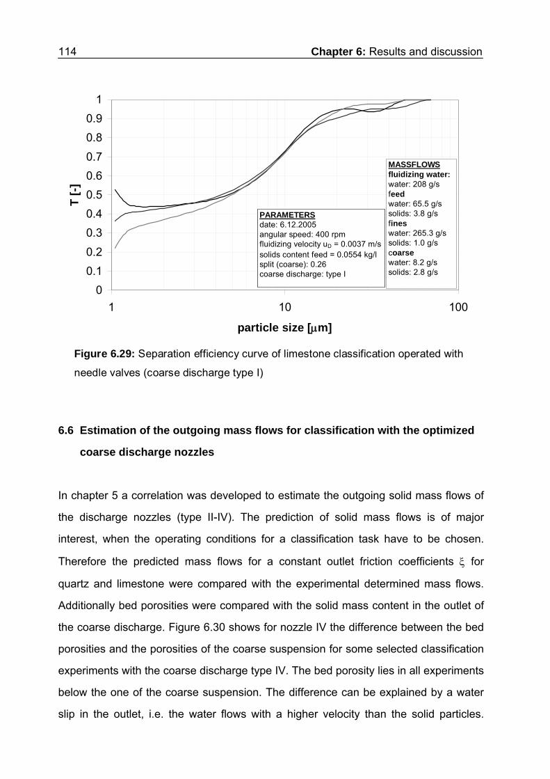
114 Chapter 6: Results and discussion
Figure 6.29: Separation efficiency curve of limestone classification operated with
needle valves (coarse discharge type I)
0
0.1
0.2
0.3
0.4
0.5
0.6
0.7
0.8
0.9
1
1 10 100
particle size [m]
T [
-]
PARAMETERSdate: 6.12.2005angular speed: 400 rpmfluidizing velocity uD = 0.0037 m/ssolids content feed = 0.0554 kg/lsplit (coarse): 0.26coarse discharge: type I
MASSFLOWSfluidizing water: water: 208 g/s feedwater: 65.5 g/ssolids: 3.8 g/sfineswater: 265.3 g/ssolids: 1.0 g/scoarsewater: 8.2 g/ssolids: 2.8 g/s
6.6 Estimation of the outgoing mass flows for classification with the optimized
coarse discharge nozzles
In chapter 5 a correlation was developed to estimate the outgoing solid mass flows of
the discharge nozzles (type II-IV). The prediction of solid mass flows is of major
interest, when the operating conditions for a classification task have to be chosen.
Therefore the predicted mass flows for a constant outlet friction coefficients for
quartz and limestone were compared with the experimental determined mass flows.
Additionally bed porosities were compared with the solid mass content in the outlet of
the coarse discharge. Figure 6.30 shows for nozzle IV the difference between the bed
porosities and the porosities of the coarse suspension for some selected classification
experiments with the coarse discharge type IV. The bed porosity lies in all experiments
below the one of the coarse suspension. The difference can be explained by a water
slip in the outlet, i.e. the water flows with a higher velocity than the solid particles.

Chapter 6: Results and discussion 115
Figure 6.30 shows for higher angular velocities a higher difference between bed and
coarse suspension porosity or in other words a higher fluid slip. With decreasing bed
porosity and decreasing angular velocity the water slip decreases also. The slip in the
coarse discharge is difficult to predict and a detailed study is needed to model it, what
is not part of this work. The slip is influencing the apparent viscosity in the nozzle and
the viscosity is influencing the outgoing currents. Therefore the laminar content is not
considered in the modeling of the solid mass flow out of the bed, instead the general
formula proposed in chapter 5.6.4 is used.
Figure 6.30: Comparison of the porosities in the fluidized bed and in the coarse
outlet suspension with the discharge nozzle type 4.
0.70
0.72
0.74
0.76
0.78
0.80
0.82
0.84
0.86
0.550 0.575 0.600 0.625 0.650 0.675 0.700
bed porosity [-]
coar
se d
isch
arg
e p
oro
sity
[-]
24.4.2008 (400 rpm)28.4.2008(400 rpm)
29.4.2008 (400 rpm)
8.5.2008 (400 rpm)
23.5.2008 (700 rpm)
21.5.2008 (600 rpm)
Table 6.1 gives the experimental data of different classification experiments conducted
with the discharge nozzle type IV. The pure water mass flows of the suspension S, the
fines F and the coarse suspension C are given as well as the solid mass flows

116 Chapter 6: Results and discussion
(coarse: ; fines: F . xF; feed: S . xS). Nozzle friction coefficients for quartz = 2.7
and for limestone = 5 were determined by adaptation to the experimental data for the
model proposed in chapter 5, which is also valid for the nozzles II and III. Comparing
the columns of the experimentally determined solids mass flows out of the coarse
discharge nozzle with the calculated data, it can be seen that the values are quite in a
good agreement, so that the model can be assessed as precise enough for a first
estimation of the outgoing mass flows for the nozzles used in this work.
CM
The cut size can be calculated from the force balance on a single particle and is
illustrated in figure 6.31, where cut sizes are plotted versus classifying water
throughput depending on rotational velocity and density difference. The presented
findings enable the selection of appropriate operating conditions as described in
chapter 5.6.
Table 6.1: Comparison between calculated and experimentally determined mass flow
through the coarse discharge nozzle type IV

Chapter 6: Results and discussion 117
Figure 6.31: Cut sizes calculated from a force balance on the single sphere
depending on the operating conditions
0
5
10
15
20
25
0.0 0.5 1.0 1.5 2.0
classifying water throughput [m3/h]
cut
size
[m
]
[kg/m3]
500100020005000
400 rpm
0
5
10
15
20
25
0.0 0.5 1.0 1.5 2.0
classifying water throughput [m3/h]
cut
size
[m
]
[kg/m3]
50010002000
500 rpm
5000
0
5
10
15
20
25
0.0 0.5 1.0 1.5 2.0
classifying water throughput [m3/h]
cut
size
[m
]
[kg/m3]
700 rpm
500020001000500

118 Chapter 6: Results and discussion
6.7 Classification experiments with the optimized coarse discharge
Because of poor separation performance the coarse discharge type 1 was replaced by
the coarse discharge nozzle, in the first case (type II) an outlet pipe with a diameter of
1 mm located 1.3 cm above the distributor (cf. figure 5.7). The experiment
(13.10.2006) with the new coarse discharge was operated at similar conditions (400
rpm, 3 g/s solid feed rate) as with type I. The classification experiment (figure 6.32)
revealed a strong fishhook and a misclassification of coarse particles. For clarification
a closer look into bed build up was taken. Figure 6.33 shows the development of the
bed height during the experiment. In the first minutes the bed height was increasing
until it was approaching the coarse discharge. Reaching the height of the coarse
discharge the bed height remains constant. This indicates that the coarse discharge
nozzle was not completely submerged in the fluidized bed. To further support this
conclusion the coarse discharge flow was estimated with the help of equation (5.55)
with a bed height of 1.5 cm and a pressure drop coefficient = 2.7. With a calculated
solid mass flow of = 3.1 g/s through the discharge nozzle, the calculated value
exceeds the measured one significantly. The calculated one is based on the
assumption of a completely submerged discharge, which is obviously not fulfilled in
this case. In other words, a mass flow of = 3.1 g/s into the fluidized bed would be
necessary for the given conditions to keep the bed height at a minimal level above the
coarse discharge. If the real flow is lower, the coarse discharge penetrates into the
freeboard and a bypass of fines and vortices in the freeboard occur as with the coarse
discharge type 1 (chapter 6.5) resulting in an insufficient classification efficiency. A cut
size of dC = 9 m and a coarse fraction c = 0.52 was measured for this configuration.
CM
CM
With an increase of the mass flow into the bed by an increase of the solids
concentration in the suspension feed a submerged coarse discharge can be assured.
In the classification experiment (21.9.2006) shown in figure 6.34, conducted at 400
rpm and 0.0033 m/s fluidizing velocity, a mass flow of 4.3 g/s into

Chapter 6: Results and discussion 119
Figure 6.32: Separation efficiency curve of quartz classification operated with coarse
discharge nozzle (type II)
Figure 6.33: Bed height diagram of quartz classification (13.10.2006)
0.0
0.5
1.0
1.5
2.0
2.5
3.0
3.5
4.0
0 10 20 30 40 50time [min]
hei
gh
t o
f th
e fl
uid
ized
bed
[cm
]
feed
shu
tdow
n
level of coarse discharge (type II)
sampling times
0
0.1
0.2
0.3
0.4
0.5
0.6
0.7
0.8
0.9
1
1 10 100particle size [m]
T [
-] 1st sample2nd sample3rd sample
MASSFLOWSFluidizing water: water: 186 g/s Feedwater: 54 g/ssolids: 3.0 g/sFineswater: 210 g/ssolids: 1.4 g/sCoarsewater: 30 g/ssolids: 1.6 g/s PARAMETERS
date: 13.10.2006angular speed: 400 rpmfluidizing velocity uD = 0.0033 m/ssolids content feed = 0,055 kg/lsplit (coarse): 0.52coarse discharge: type II

120 Chapter 6: Results and discussion
the fluidized bed was reached. The submersion of the coarse discharge increases the
separation performance significantly. The misclassification of the coarse particles
indicated by a local minimum at 40 m in figure 6.32 was vanished and the fishhook
effect eliminated. The slope of the separation efficiency curve was strongly increased,
which indicates a sharp separation. After the definition of Eder a sharpness = 0.63 is
reached, what lies in the range of industrial sharp separations. In the fines region just
a small amount particles have been misclassified, what is in the range of acceptance
for industrial application. In this case the coarse fraction c = 0.45 is reduced compared
to the previous experiment as less fines are been misclassified. The reduction of the
coarse fraction increases the cut size to 12 m.
It has to be noted that the separation efficiency curves of the 4 samples taken at
different times are almost identical, so that stationary conditions were prevailing. The
times of sampling can be taken out of the bed height diagram (figure 6.35).
In this experiment a constant bed height of approximately 1.2 cm above the coarse
discharge is achieved after 18 minutes, i.e. an equilibrium between the solid mass
flows into the bed and out of the coarse discharge is reached. After shutdown of the
suspension feed after 42 minutes of classification the bed height is quickly reduced to
the level of the coarse discharge. The calculation of the coarse discharge flow leads to
a solids mass flow of = 4.5 g/s, what is in a good agreement with the experimental
value of 4.3 g/s.
CM

Chapter 6: Results and discussion 121
Figure 6.34: Separation efficiency curve of quartz classification operated with coarse
discharge nozzle type II (21.9.2006)
0.0
0.5
1.0
1.5
2.0
2.5
3.0
3.5
4.0
0 10 20 30 40 50time [min]
hei
gh
t o
f th
e fl
uid
ized
bed
[c
m]
sampling times
level of coarse discharge (type II)
feed
shu
tdow
n
Figure 6.35: Bed height diagram of quartz classification (21.9.2006)
0
0.1
0.2
0.3
0.4
0.5
0.6
0.7
0.8
0.9
1
1 10 100particle size [m]
T [
-] 1st sample
2nd sample
3rd sample
4th sample
MASSFLOWSFluidizing water: water: 186 g/s Feedwater: 52 g/ssolids: 9.5 g/sFineswater: 231 g/ssolids: 5.2 g/sCoarsewater: 7 g/ssolids: 4.3 g/s
PARAMETERSdate: 21.9.2006angular speed: 400 rpmfluidizing velocity uD = 0.0033 m/ssolids content feed = 0,17 kg/lsplit (coarse): 0.45coarse discharge: type II

122 Chapter 6: Results and discussion
6.8 Classification experiments with the coarse discharge nozzle type III
The replacement of the coarse discharge mechanism (type I) by the discharge nozzle
type II brought an improvement of the control of the outgoing currents, a realization of
a constant bed height and of course an increase of the separation performance. The
discharge nozzle type II was not penetrating into the bed, but was arranged in the side
wall of the classification chamber. To analyze the influence of the location of the
discharge nozzle, it was brought into the center of the classification chamber (nozzle
type III) and classification experiments were performed. Figure 6.36 shows the results
of the classification experiment (19.3.2008) under comparable conditions as the
experiment with the discharge nozzle II (21.9.2006). The bed height diagram is
pictured in figure 6.37. The 4 samples taken at different times, when a constant bed
height was reached, show a small deviation, what lies in the range of experimental
precision. The average cut size dC = 11 m is comparable with the classification with
nozzle II. The sharpness = 0.58 as well as the bed height is below the ones of the
experiment from the 21.9.2006. It is not clear if the lower sharpness is due to the
arrangement of the discharge nozzle, which might disturb the flow or has it to be
contributed to the influence of the bed height, what will be discussed later.
The constancy of the bed height at a lower level for the coarse discharge nozzle III can
be explained by a difference of the fluidization in the center compared to the wall. In
the center a well fluidized bed can be assumed, while at the wall the flow is reduced by
wall friction, resulting in a lower porosity at the wall compared to the center. Thus the
apparent viscosity in the center is lower than at the wall, what eases the outflow in the
center. Therefore a lower bed height is adjusted. However, an increase of the
separation efficiency is not achieved by this configuration compared to nozzle II, so
that nozzle III was not investigated further.

Chapter 6: Results and discussion 123
Figure 6.36: Separation efficiency curve of quartz classification operated with coarse
discharge nozzle type III (19.3.2008)
Figure 6.37: Bed height diagram of quartz classification (19.3.2008)
0.0
0.5
1.0
1.5
2.0
2.5
3.0
3.5
4.0
0 10 20 30 40 50
time [min]
hei
gh
t o
f th
e fl
uid
ized
bed
[cm
]
sampling times
feed
shu
tdow
n
level of coarse discharge (type III)
0.0
0.1
0.2
0.3
0.4
0.5
0.6
0.7
0.8
0.9
1.0
1 10
particle size [m]
T [
-]
100
1st sample2nd sample3rd sample4th sample
PARAMETERSdate: 19.3.2008angular speed: 400 rpmfluidizing velocity uD = 0.0033 m/ssolids content feed = 0,197 kg/lsplit (coarse): 0.47coarse discharge: type III
MASSFLOWSFluidizing water water: 183 g/s Feedwater: 46 g/ssolids: 9.8 g/sFineswater: 224 g/ssolids: 5.2 g/sCoarsewater: 5 g/ssolids: 4.6 g/s

124 Chapter 6: Results and discussion
6.9 Classification with the coarse discharge nozzle type IV
To study the influence of the position of the outlet orifice, coarse discharge IV was
developed. The nozzle is arranged such that the orifice is facing the distributor at a
distance of 5 mm. The orifice nozzle is connected to the outlet transport pipe at a 90°
angle (cf. figure 5.7). The design of coarse discharge IV enhances the distance from
the bed surface to the outlet, what should make it more difficult for the fines to be
misclassified. With the discharge nozzle IV the influence of the bed height, the
suspension feed concentration and the cut size on the separation efficiency were
investigated. As mentioned above classification is only recommended above 1.5 x umf
and therefore the presented results were conducted in the range 1.5 x umf< u < 4 x umf.
When performing classifications with coarse discharge nozzle IV it was always
assured that the nozzle was completely covered by the bed to avoid bypass of fines.
Figure 6.38 shows the classification with the nozzle IV (24.4.2008) for a cut size of dC
= 13 m at 400 rpm and with a fluidizing velocity of uD = 2.1 x umf. A high separation
sharpness of dp,25/dp,75 = 0.62 was achieved. The amount of fines below 8 m been
misclassified is smaller compared to the experiments with other coarse discharges, i.e.
the coarse fraction contains only a very tiny amount of fines, while the fines fraction is
completely devoid of particles larger than 23 m. However the sharpness is
comparable with the result obtained with nozzle II (21.9.2006). The separation
efficiency curves of 5 taken samples are presented in figure 6.38 and all of them show
a very small deviation from the others, so that stationary conditions can be assumed.
Also the bed height as shown in figure 6.39 stays almost constant after 25 minutes, so
that an equilibrium between particles entering the bed from the coarse fraction of the
suspension feed and leaving the bed through the nozzle was reached. The bed height
was adjusted between 1.3 to 1.4 cm above the distributor or 0.8 to 0.9 cm above the
nozzle orifice.

Chapter 6: Results and discussion 125
0.0
0.5
1.0
1.5
2.0
2.5
3.0
3.5
4.0
0 10 20 30 40 50
time [min]
hei
gh
t o
f th
e fl
uid
ized
bed
[cm
]
sampling times
feed
shu
tdow
n
level of coarse discharge (type IV)
Figure 6.38: Separation efficiency curve of quartz classification operated with coarse
discharge nozzle type IV (24.4.2008)
Figure 6.39: Bed height diagram of quartz classification (24.4.2008)
0.0
0.1
0.2
0.3
0.4
0.5
0.6
0.7
0.8
0.9
1.0
1 10 100
particle size [m]
T [
-]
1st sample2nd sample3rd sample4th sample5th sample
MASSFLOWSFluidizing water water: 244 g/s Feedwater: 46 g/ssolids: 10.2 g/sFineswater: 286 g/ssolids: 6.4 g/sCoarsewater: 4 g/ssolids: 3.8 g/s PARAMETERS
date: 24.4.2008angular speed: 400 rpmfluidizing velocity uD = 0.0044 m/ssolids content feed = 0,169 kg/lsplit (coarse): 0.38coarse discharge: type IV

126 Chapter 6: Results and discussion
6.9.1 Influence of the bed height
As coverage of the discharge nozzle by the fluidized bed is essential for the
classification, the question arises how the bed height influences the classification
performance even when the nozzle is covered. For that reason a classification was
carried out with increasing bed height (28.4.2008), the results are depicted in figure
6.40. With increasing bed height the experiment becomes instationary, i.e. particles
were accumulated in the bed. For the calculation of the mass flows for the
determination of the separation efficiency curve the equations (5.64 – 5.65) were
employed, taking the accumulation of the particles in the bed into account. The
accumulation was determined by the change of the bed height. The build up of the bed
was conducted with comparable conditions as in the experiment of the 24.4.2008, but
with a fluidizing velocity of 0.0031 m/s. Due to this more particles are classified to the
coarse fraction. The consequence is that more particles report to the fluidized bed than
the outlet nozzle can handle for bed heights below 4 cm above the distributor. Thus
the bed height increases due to accumulation of particles. The separation efficiency
and the corresponding development of the bed height of the described experiment are
presented in the figures 6.40 and 6.41. The bed height increases as expected to a
level above the suspension feed port and samples were taken when an approximately
constant increase of the solids mass of 0.9 g/s took place. The bed heights of samples
1 and 2 were below the 4 feed ports, which have diameters of 0.5 cm and the centers
are located 3.25 cm above the distributor. For the samples 3 and 4 the bed heights
reached the positions of the feed ports, so that it can be assumed that the complete
suspension feed was injected to the fluidized bed. For the understanding of the
classification it is interesting to know how this influences the classification. From figure
6.40 it can be seen that with increasing bed height the separation efficiency curves are
shifted to coarser diameters. The sharpness of the classification increases significantly
from = 0.57 at a bed height of HB = 2.4 cm to = 0.67 at HB = 3.2 cm.

Chapter 6: Results and discussion 127
0.0
0.1
0.2
0.3
0.4
0.5
0.6
0.7
0.8
0.9
1.0
1 10 100
particle size [m]
T [
-]
MASSFLOWS1st sample
0.0
0.5
1.0
1.5
2.0
2.5
3.0
3.5
4.0
0 10 20 30 40 50
time [min]
hei
gh
t o
f th
e fl
uid
ized
bed
[cm
]
height of suspension feed
coarse discharge
Figure 6.40: Separation efficiency curve of quartz classification depending on the
bed height (28.4.2008)
Figure 6.41: Bed height diagram of quartz classification (28.4.2008)
2nd sample3rd sample4th sample
Fluidizing water water: 173 g/s Feedwater: 46 g/ssolids: 10.7 g/sFineswater: 213 g/ssolids: 4.8 g/sCoarsewater: 6 g/ssolids: 5.0 g/sAv. bed accumulationsolids: 0.9 g/s
PARAMETERSdate: 28.4.2008angular speed: 400 rpmfluidizing velocity uD = 0.0031 m/ssolids content feed = 0.210 kg/lsplit (coarse): 0.53coarse discharge: type IV

128 Chapter 6: Results and discussion
The cut size was shifted from dC = 9 m to 11 m, for the samples 3 and 4 both the cut
sizes and the sharpness stay almost the same. It can therefore be concluded that
increasing the bed height increases the slope of the separation efficiency curve, while
shifting the cut size to higher particle diameters.
This experiment provides also a deeper insight into the classification process. As the
bed height reaches the position of the feed ports, the whole suspension containing
fines and coarse particles is introduced into the fluidized bed, i.e. the fines cannot be
separated in the freeboard. In a gas fluidized bed an almost complete mixing of
particles inside the bed would be observed, which, however, cannot be the case for
wet centrifugal classification, because a sharp classification was achieved even when
the whole suspension flow is introduced into the bed. On the contrary the amount of
fines reported to the nozzle was reduced with increasing bed height, which can only be
explained by a strong segregation above the height of the fluidized bed. In case of the
bed height reaching to the feed ports (sample 4) a particle size distribution of the raw
material can be assumed at the bed surface, which changes along the bed height
down to the nozzle to final coarse particle size distribution.
The influence of the bed height was also studied for the classification of cut sizes
below 10 m. Figure 6.42 pictures the classification experiment (29.4.2008), where the
bed height was increased from 1 to 4 cm above the distributor. With a fluidizing
velocity of uD = 0.002 m/s the coarse discharge was not capable to completely
discharge the coarse fraction, so that the fluidized bed was built up. The fluidizing
velocity, which equals approximately 1.5 times the minimum fluidizing velocity (uD =
1.5 x umf) is in the range of recommendation. The separation performance is
technically sharp for all samples taken and ranges between = 0.52 at the low bed
height of HB = 1 cm to = 0.67 at a bed height of HB = 4 cm. Cut sizes between 6 and
10 m were achieved. At the highest bed height the suspension is injected directly into

Chapter 6: Results and discussion 129
the fluidized bed and the cut size as well as the sharpness is the highest, what
confirms the findings presented above.
Figure 6.42: Separation efficiency curve of quartz classification depending on the
bed height with cut sizes below 10 m (29.4.2008)
0.0
0.1
0.2
0.3
0.4
0.5
0.6
0.7
0.8
0.9
1.0
1 10
particle size [m]
T [
-]
100
1st sample2nd sample3rd sample4th sample
PARAMETERSdate: 29.4.2008angular speed: 400 rpmfluidizing velocity uD = 0.002 m/ssolids feed content = 0.210 kg/lsplit (coarse): 0.58coarse discharge: type IV
MASSFLOWSFluidizing water water: 111 g/s Feedwater: 46 g/ssolids: 9.8 g/sFineswater: 150 g/ssolids: 3.7 g/sCoarsewater: 7 g/ssolids: 4.8 g/sAv. Bed accumulationsolids: 1.3 g/s
6.9.2 Effect of the number of feed ports on the classification with nozzle IV
Due to a strong tangential flow in the freeboard induced by the Coriolis force, the
injected suspension feed is immediately distributed circumferentially in classification
chamber. It can be expected that this will also happen when the four feed ports are
replaced by only one. In this case the injected flow through the single port is four times
higher than in the four feed ports. Considering only a single feed port is a simplification
for the design, which is advantageous for industrial usage. For that reason an
experiment was conducted with only one active feed port (8.5.2006). Figure 6.43
shows the setup. On top the configuration with the four open ports and the single
coarse discharge as used before is presented. At the bottom only one feed and one

130 Chapter 6: Results and discussion
coarse discharge nozzle is visible. As the bed and the freeboard moves tangentially in
the direction of rotation the injected particles are expected to follow the flow inside the
classifier. For that reason the open feed port is located shortly behind the coarse
discharge nozzle to enhance the minimum traveling distance of a single particle, i.e. a
particle has at least to perform an almost complete rotation before it can report to
coarse discharge nozzle. The intention is the reduction of misclassification of fines by
enhancing the minimum tracking distance.
Figure 6.43: Classification with only one suspension feed port
30°
vtan
suspension feed
coarse discharge
minimal particle trackin the classification chamber
30°
vtan
minimal particle trackin the classification chamber
coarse dischargesuspension feed
Classification with 4 suspension feedports
Classification with 1 suspension feedport
To study the influence of the bed height in this configuration, similar conditions were
chosen as in the experiment at the 28.4.2008. Quartz particles were injected to the
single feed port at 400 rpm and fluidized at 3.1 mm/s. 47 % of the solids feed were
classified to the fines and 45 % to the coarse fraction. An average of 8 % of the solids

Chapter 6: Results and discussion 131
feed was accumulated in the fluidized bed, where at the beginning the accumulation
was stronger than at the end of the experiment. The build up of the fluidized bed is
shown in figure 6.44. The samples were taken at different bed heights for further
clarification of the influence of the bed height on the separation efficiency.
The separation efficiency curves are shown in figure 6.45. Different cut sizes were
achieved, ranging from 9 to 12 m depending on the bed height, which was increased
from 1.5 cm to 3 cm above the distributor. With increasing bed height, the separation
efficiency curve was shifted to the coarse region with achieving higher separation
sharpness . The range of the separation sharpness is between 0.55 < < 0.68, which
can be classified as technically sharp separation. The amount of fines is for all cases
very small, however a minimum of misclassified particles can be found in the sample
of the largest bed height.
These findings are confirming the results of the previous experiment conducted at the
28.4.2009. Also the separation sharpness and the cut size for this case are
comparable, what indicates that the injection of the suspension by one single feed port
is sufficient and a higher number of feed ports is overrated. However, the following
classification experiments were conducted with four active feed ports.

132 Chapter 6: Results and discussion
0.0
0.5
1.0
1.5
2.0
2.5
3.0
3.5
4.0
0 10 20 30 40 50
time [min]
hei
gh
t o
f th
e fl
uid
ize
d b
ed [
cm]
sampling times
level of coarse discharge (type IV)
feed
shu
tdow
nFigure 6.44: Bed height diagram of quartz classification (8.5.2008)
0.0
0.1
0.2
0.3
0.4
0.5
0.6
0.7
0.8
0.9
1.0
1 10 100
particle size [m]
T [
-]
1st sample2nd sample3rd sample4th sample5th sample6th sample
PARAMETERSdate: 8.5.2008angular speed: 400 rpmfluidizing velocity uD = 0.0031 m/ssolids content feed = 0,197 kg/lsplit (coarse): 0.50coarse discharge: type IV
MASSFLOWSFluidizing water water: 173 g/s Feedwater: 46 g/ssolids: 10.0 g/sFineswater: 214 g/ssolids: 4.7 g/sCoarsewater: 5 g/ssolids: 4.5 g/sAv. bed accumulationsolids: 0.8 g/s
Figure 6.45: Separation efficiency curve of quartz classification depending on the
bed height with only one suspension feed open (8.5.2008)

Chapter 6: Results and discussion 133
6.9.3 Classification of limestone
Limestone is like quartz a natural product, which is therefore irregular shaped.
Although the density (Li = 2620 kg/m3) and the particle size distribution of the used
limestone is similar to quartz, the fluidized bed expansion behavior differs significantly
from quartz (Margraf and Werther, 2008). The investigation of the feasibility of the
classification of limestone with the optimized coarse discharge is therefore of big
interest. In figure 6.46 the result of limestone classification of 10th April is presented. A
high fluidized bed was achieved, whose height reached constancy at 3.9 cm above the
distributor at the end of the sampling period. The coarse discharge as well as the
suspension feed ports were submerged by the fluidized bed. This applies to all taken
samples during the sampling period, in which the bed height was increased from 3.2
cm to its final and stationary height of 3.9 cm. For all samples a very sharp separation
performance with = 0.77 was achieved, which confirms the finding that a high
fluidized bed is favorable for the classification. Also for limestone a strong segregation
in the bed from the submerged coarse discharge to the submerged feed ports can be
assumed. At 400 rpm with a fluidizing velocity of 4.4 mm/s cut sizes between 16 and
18 m depending on the bed height were achieved. With limestone a slight increase of
the cut size can be observed with increasing bed height. This behavior is similar to the
one observed with quartz. The bed height reached higher values at similar conditions
compared to quartz due to a higher bed voidage, which was investigated by Margraf
and Werther (2008).

134 Chapter 6: Results and discussion
Figure 6.46: Separation efficiency curve of limestone classification with a cut size of
about 20 m (10.4.2008)
0.0
0.1
0.2
0.3
0.4
0.5
0.6
0.7
0.8
0.9
1.0
1 10 100
particle size [m]
T [
-] 1st sample at 3.2 cm bed height2nd sample at 3.5 cm bed height3rd sample at 3.8 cm bed height4th sample at 3.9 cm bed height
MASSFLOWSFluidizing water water: 247 g/s Feedwater: 47 g/ssolids: 8.3 g/sFineswater: 292 g/ssolids: 6.1 g/sCoarsewater: 2 g/ssolids: 2.2 g/s
PARAMETERSdate: 10.4.2008angular speed: 400 rpmfluidizing velocity uD = 0.0044 m/ssolids content feed = 0.168 kg/lsplit (coarse): 0.27coarse discharge: type IV
6.9.4 Classification of quartz for cut sizes between 1 and 10 m
With increasing angular velocities above 600 rpm cut sizes far below 10 m can be
achieved. As quartz powder ranges from 1 to 60 m with only mass-20 % below 4 m,
classifications below 4 m are not recommendable for this material. Furthermore at
lower cut sizes the stable fluidization of the larger particles cannot be assured.
Therefore classification experiments with cut sizes of approximately 6 and 4.7 m
were carried out. It should be mentioned that particle collectives containing submicron
particles can be classified at cut sizes down to 1 m and below, when the
classification is not disturbed by defluidized zones due to the presence of too large
particles.

Chapter 6: Results and discussion 135
The separation efficiency curves of figure 6.47 are showing the classification results at
600 rpm for a cut sizes at approximately 6 m. The curves are corresponding to
samples, taken in a time range of 30 minutes at a constant bed height of 2.2 cm. The
deviations of the cut sizes and the shapes of the curves are very small, so that
stationary conditions can be assumed. With = 0.5 a technically sharp classification
was achieved. A similar result gives the classification experiment conducted at 700
rpm and at a cut size of 4.7 m (figure 6.48). Stationary conditions were achieved
when the bed height reaches 1.8 cm and samples were taken over 20 minutes of
operation. A sharpness of = 0.51 was reached which is comparable to the one
presented above. The performance of the classification in the range of cut sizes below
10 m is still technically sharp and no fishhook effect can be observed.
Figure 6.47: Separation efficiency curve of fine quartz classification at a constant
bed height of 2.2 cm (21.5.2008)
0.0
0.1
0.2
0.3
0.4
0.5
0.6
0.7
0.8
0.9
1.0
1 10 100
particle size [m]
T [
-]
1st sample2nd sample3rd sample4th sample
MASSFLOWSFluidizing water water: 174 g/s Feedwater: 46 g/ssolids: 9.8 g/sFineswater: 209 g/ssolids: 3.3 g/sCoarsewater: 10 g/ssolids: 6.5 g/s PARAMETERS
date: 21.5.2008angular speed: 600 rpmfluidizing velocity uD = 0.0031 m/ssolids content feed = 0,212 kg/lsplit (coarse): 0.66coarse discharge: type IV
However, the sharpness of the classification is smaller compared to cut sizes above
10 m. An explanation is that with decreasing cut sizes the range of particle diameters

136 Chapter 6: Results and discussion
in the fluidized bed is increased, which may lead to an onset of defluidized zones in
the bed. These instabilities may contribute to a decrease in the classification
performance.
Figure 6.48: Separation efficiency curve of fine quartz classification at a constant
bed height of 1.8 cm (23.5.2008)
0.0
0.1
0.2
0.3
0.4
0.5
0.6
0.7
0.8
0.9
1.0
1 10 100
particle size [m]
T [
-]
1st sample2nd sample3rd sample4th sample
MASSFLOWSFluidizing water water: 174 g/s Feedwater: 46 g/ssolids: 10.8 g/sFineswater: 203 g/ssolids: 3.0 g/sCoarsewater: 17 g/ssolids: 7.8 g/s PARAMETERS
date: 23.5.2008angular speed: 700 rpmfluidizing velocity uD = 0.0031 m/ssolids content feed = 0.235 kg/lsplit (coarse): 0.27coarse discharge: type IV
6.9.5 Classification of glass beads
Finally the influence of the particle shape was investigated. Therefore the separation
efficiency of a classification of spherical shaped particles (glass beads, cf. figure 5.1
and 5.2) was determined.
As only 10-mass% of the glass beads are below 20 m, cut sizes above 20 m are
necessary to obtain reasonable results. The classification experiment presented in
figure 6.49 shows a cut size of 21 m. With a coarse fraction of c = 0.85 only 15% of

Chapter 6: Results and discussion 137
the raw material was elutriated to the overflow. For the classification a rotational speed
of 185 rpm was adjusted with a fluidizing velocity of 2.8 mm/s at the distributor. The
bed reached after 10 minutes a stationary height of 1.9 cm and samples were taken. It
can be seen that a high slope of the separation efficiency curve was achieved. A
sharpness of = 0.91 was achieved and no fishhook effect can be observed. This
high separation efficiency can be explained by a very smooth fluidization of a bed with
a very narrow particle size distribution. Furthermore the spherical shape of the glass
particle gives ideal conditions for fluidization and for the transport to the coarse and
fines discharge. Thus an almost ideal classification was achieved.
Figure 6.49: Separation efficiency curve of glass beads classification at a constant
bed height of 1.90 cm (18.9.2008)
0.0
0.1
0.2
0.3
0.4
0.5
0.6
0.7
0.8
0.9
1.0
1 10
particle size [m]
T [
-]
100
1st sample
2nd sample
PARAMETERSdate: 18.9.2008angular speed: 185 rpmfluidizing velocity uD = 0.0028 m/ssolids content feed = 0.11 kg/lsplit (coarse): 0.85coarse discharge: type IV
MASSFLOWSFluidizing water water: 158 g/s Feedwater: 48 g/ssolids: 5.0 g/sFineswater: 203 g/ssolids: 0.8 g/sCoarsewater: 3 g/ssolids: 4.2 g/s

138 Chapter 6: Results and discussion
6.10 Practical example of the control strategies for quartz powder classification
In the previous chapters the classification process of the present classifier was
discussed in detail and the results of the investigations were presented. Finally the
findings will now be used to design a classification process with the classifier of the
present work.
For the given material, which is to be classified with the certain cut size dC, a rotational
speed and the bed height in the classifier are chosen. The necessary fluidizing velocity
and the permissible feed mass flow are calculated. An estimation of the minimum
fluidizing velocity umf will prove the feasibility of the given classification task, i.e. when
u > 1.5 x umf.
As an example the quartz powder with the properties presented in chapter 5.1 was
selected as the material to be classified. A cut size with a diameter of dC = 7 m was
chosen. Under the assumption of an ideal classification, the fines fraction f, the coarse
fraction c and their cumulative mass distributions Q3,F(dp), Q3,C(dp) are given due to the
cut size dC and the feed mass distribution Q3,S (dp) by:
f = Q3,S(dC) (6.5)
c = 1 – f (6.6)
Q3,F(dp) = Q3,S(dp)/f; for dp < dC (6.7)
Q3,C(dp) = [Q3,S(dp) –Q3,S(dC)]/c; for dp > dC (6.8)
For the present case f = 0.4 and c = 0.6 are obtained, the cumulative mass
distributions of the feed, fines and coarse fraction are shown in figure 6.50. Under the
assumption that the coarse mass distribution equals the one of the fluidized bed, a
median diameter of dp,50 = 16 m and a Sauter diameter of d32 = 15 m for the
fluidized bed are obtained.

Chapter 6: Results and discussion 139
For classifications with cut sizes below 10 m rotational velocities larger than 400 rpm
are recommendable. For the present case 500 rpm were chosen to be suitable. A
higher rotational speed would result in an unnecessarily high throughput of fluidizing
water. For bed heights of 3.0 cm and above, sharp classifications were obtained (cf.
experiments 28.4.2008 and 8.5.2008, figures 6.40 and 6.45), so that a target bed
height of 3.5 cm was selected, i.e. the surface of the fluidized bed is RB = 0.41 m.
From figure 5.8 the terminal velocity of the fluidized bed can now be taken with ut =
0.020 m/s.
Applying equations (5.58), (5.57) and (5.39) gives the fluidizing velocity u, the bed
porosity and the mass of solids mS in the fluidized bed:
fluidizing velocity: u = 0.0042 m/s
bed porosity: = 0.71
solids mass in the bed: mS = 1.58 kg
For the given solids mass mS, the theoretical fixed bed height HFB = 2.1 cm or the
radius of the fixed bed surface RFB = 0.424 m are calculated by equation (5.36) under
the assumption of a fixed bed porosity of 0.5 (cf. figure 6.19).
The equations (5.37) and (5.45) allow the estimation of the pressure drop profile,
which is pictured in figure 6.51. A minimum fluidizing velocity of umf = 0.0007 m/s is
obtained. The ratio u/umf is then
mf
u 0.0042 m/ s6
u 0.0007 m/ s umf > 1.5
This means that the feasibility of the classification process is proven.

140 Chapter 6: Results and discussion
Figure 6.50: Cumulative mass distributions of the feed, the coarse and the fines
fraction for an ideal quartz powder classification with the cut size dC = 7 m
Figure 6.51: Calculated pressure drop profile for the example of quartz classification
at 500 rpm with a cut size dC = 7 m and a fluidizing velocity uD = 0.0042 m/s
0
10
20
30
40
50
60
70
80
90
100
1 10 100particle size [m]
Q3
[%
]
quartz powder - feedquartz powder - finesquartz powder - coarse
cut size
0
5000
10000
15000
20000
25000
30000
0 0.001 0.002 0.003 0.004 0.005fluidizing velocity [m/s]
pre
ssu
re d
rop
[P
a]
fixed bed
fluidized bed
umf u

Chapter 6: Results and discussion 141
With the discharge nozzle (IV) with an orifice diameter of dN = 1 mm, equations (5.55)
and (5.56) give the coarse discharge suspension and solids mass flow:
SUS,CM
CM
= 9.1 g/s
= 4.5 g/s
The required solids feed mass flow is then given by
CS
MM 7.5 g/ s
c (6.9)
It should be noted that the target bed height is in fact controlled via the feed mass flow.
For the given case a tolerance interval of ±0.5 cm from the target bed height is
acceptable. The radius of the fluidized bed surface is correlated via equation (5.38)
with the bed pressure drop, whereby the radius RB of the bed can be calculated even
when the bed height cannot be determined optically due to turbidity. In figure 6.52 the
bed pressure drop is plotted versus the bed height for the present case. The ideal
operation point and the acceptable tolerance interval are provided to ensure a high
sharpness and a constant cut size. Via figure 6.52 the operator is provided with the
valuable information about the operating status of his classification process. The
easiest way to keep the pressure drop and thus the bed height at the desired level is
to adjust the feed mass flow accordingly.

142 Chapter 6: Results and discussion

7 Summary and Conclusions
A centrifugal counter current classifier was investigated and optimized. The classifier
can be operated continuously and is designed for wet classification in the micron
range. The principle of the classifier is based on gravity elutriation but is transferred
to the centrifugal field. The fluid mechanics were analyzed experimentally and with
CFD simulations.
First tests in the solids-free chamber revealed an intense tangential flow in the
direction of rotation, which is caused by the Coriolis force, resulting from the radial
flow of the liquid. Also air shows a high tangential velocity under similar conditions
but with lower tangential velocities due to a higher effect of the wall friction.
Numerical simulations of the liquid flow field are confirmed by measurements in a
pilot-scale apparatus. The tangential velocity is significantly higher than the radial
fluid velocity. When the chamber is filled with particles a liquid fluidized bed is set up.
In its freeboard the intense tangential flow is detected again. The fluidized bed itself
is also moving in the tangential direction, however, with a much lower velocity than
the freeboard. But even in the fluidized bed, the tangential velocities relative to the
rotating apparatus are significantly higher than the radial ones. The bed expansion of
the fluidized bed can be described by a Richardson-Zaki type power law. The
Richardson-Zaki exponents have values n of 4.9 (glass beads), 4.5 (quartz) and 5.9
(limestone) for the presently investigated particles with mean particle sizes around 30
m. The findings are useful for designing a new coarse discharge mechanism.
As the tangential bed movement is still significant it can be concluded that a single
coarse discharge is sufficient. Thus the previously installed four needle valves were
replaced by a single coarse discharge nozzle. A constant bed height could now be

144 Chapter 7: Summary and Conclusions
achieved with an equilibrium of bed height and coarse outlet flow. For reaching this
equilibrium the orifice diameter of the discharge nozzle has to be adapted to the
desired coarse discharge flow or vice versa.
Pressure drop measurements were carried out to determine the onset of fluidization
and the minimum fluidizing velocity. A stable fluidization, which is achieved at
fluidizing velocities above 1.5 x umf, and a fully submerged coarse discharge were
found to be essential for a sharp classification. Classification experiments were
performed with glass beads, quartz and limestone and very sharp separations were
achieved with cut sizes down to 5 microns.
The investigation of the influence of the bed height revealed that with increasing bed
height an enhancement of the sharpness with a slight increase of the cut size occurs.
Increasing the bed height to the radius of the feed port the solid particles are directly
injected to the bed. As the classification is still sharp it can be concluded that the bed
has to be strongly segregated.
The results showed that this classifier is very capable for separation tasks in the
micron range. The fishhook effect can be almost completely eliminated, when the
classifier is operated correctly.
Comparing the rotating fluidized bed classifier with other devices it can be concluded
that the sharp separation efficiency of gravity elutriators is achieved at cut sizes in
the micron range. The fishhook effect, which is a problem with hydrocyclones, was
eliminated and misclassifications were strongly reduced compared to the previous
configuration.
145
Nomenclature
ca
Coriolis acceleration
AC, AD cross sectional area, cross sectional area of the distributor [m2]
B width of the chamber [m]
cD drag coefficient [-]
c coarse fraction [-]
C water mass flow of the coarse suspension [kg/s]
CK Kozeny constant [CK = 4]
dC cut size [m]
dh hydraulic diameter [m]
dN inner diameter of coarse discharge nozzle [m]
dp particle diameter [m]
dps Sauter diameter [m]
dts1, dts2, dts3 diameters of the tracer spheres [m]
E(dp) error function [mg/s]
f fines fraction [-]
F water mass flow of the fines suspension [kg/s]
FB, FC, FD, FW buoyancy, centrifugal, drag and wall friction force [N]
FDR, FDT, FS drag forces in radial and tangential direction, force on chord [N]
g gravity acceleration [g = 9.81 m/s2]
K chamber profile constant [K = 0.00396 m3]
KD distributor pressure drop coefficient [Pa.s/m]
HB fluidized bed height [m]
HFB height of the fixed bed [m]
L circumference [m]
LC length of the thread (tracer sphere) [m]
m mass flow [kg/s]
mS mass of the solids in the fluidized bed [kg]
146
mL mass of water in the classification chamber
mts mass of the tracer sphere [kg]
n Richardson - Zaki exponent [-]
MF, MO, MW angular momentums (incoming flow, outgoing flow, torque) [N.m]
F SM , M , M C solids mass flows of fines, feed and coarse discharge [g/s]
SUS,S SUS,CM , M mass flows of the feed and coarse suspension [g/s]
p pressure [Pa]
Q3,S(dp),Q3,C(dp), cumulative mass distributions of the feed, coarse and fines
Q3,F(dp) particles [%]
q3,S(dp),q3,C(dp), mass density distributions of the feed, coarse and fines
q3,F(dp) particles [%/m]
r radius [m]
rts, rF radial position of the tracer sphere and the chord fixing [m]
RD, RW, RB, RN radii of the distributor, the overflow weir, the bed surface and the
coarse discharge nozzle [m]
Rets, Rep Reynolds numbers (tracer sphere, particles)
S water mass flow of the suspension [kg/s]
SV specific surface of a particle collective [1/m]
T(dp) separation efficiency curve [-]
u, ut fluidizing velocity, terminal velocity [m/s]
ud fluidizing velocity at the distributor [m/s]
V water volume flow [m3/s]
VB bed volume [m3]
W fluidizing water mass flow [kg/s]
vN fluid velocity through the discharge nozzle [m/s]
vR radial fluid velocity [m/s]
vT tangential velocity (relative to the rotor) [m/s]
Vts1, Vts2 Volumes of the tracer spheres [m3]
w absolute tangential velocity (observer located outside) [m/s]

147
xS, xF, xC solids loadings of the feed, the fines and the coarse suspension
angles for evaluation of the force balances on the tracer spheres
porosity of the fluidized bed [-]
FB fixed bed porosity [-]
classification sharpness
fluid viscosity [Pa.s]
wall friction coefficient [-]
S, L densities of solids and liquid [kg/m3]
m mean fluidized bed density [kg/m3]
nozzle pressure drop coefficient
angular velocity [1/s]

148
References
Bickert, G., “Sedimentation feinster suspendierter Partikel im Zentrifugalfeld“,
Dissertation, Universität Karlsruhe (1997).
Bohl, W., „Technische Strömungslehre“, Vogel Buchverlag (1991)
CFX, „CFX Version 5.7, Reference Manual“, ANSYS Germany GmbH, Otterfing,
Germany (2004).
Colon, F., van Heuven, J., van der Laan, H., „Centrifugal Elutriation of Particles in
Liquid Suspension.”, Groves and Wyatt-Sargent(Editors): Particle Size Analysis,
pp.42-52, Bradford 9.-11.9.1970, The Society of analytical chemistry.
De Wilde, J., de Broqueville, A., “Rotating fluidied beds in a static geometry:
experimental proof of concept”, AIChE Journal, Vol.53, No.4, pp.793-810 (2007)
Dixon, “Fluid Mechanics, Thermodynamics of Turbomachinery,” 5th edition, Elsevier
Butterworth-Heinemann, Oxford, UK (1998)
Gerhart,C., “Untersuchungen zum Trennverhalten von Hydrozyklonen niedriger
Trennkorngrößen, Dissertation, Universität Erlangen (2001)
Heiskanen, K., „Particle Classification“, Chapman & Hall, London (1993)
Hidaka, N., „Correlation of solid holdup in liquid-solid fluidized bed”, Journal of
Chemical Engineering of Japan”, Vol. 27, No.5, pp. 563-570, (1994)

149
Kalck, U., Werther, J. „Zum Einsatz von Aufstromklassierern für die Aufbereitung
kontaminierter Baggerschlämme“, Aufbereitungstechnik, 31(11), pp. 593-601, (1990)
Kellerwessel, H., Zahr, P., “Nassklassierung von Erz- und Mineralsuspensionen
unterhalb 10 mm mittels Vollmantel-Zentrifugen“, Erzmetall, 32(5), pp. 227-231, (1979)
Kerkhoff, T. „Feinkornklassierung in einem luftkernlosen Hydrozyklon“, Dissertation,
Universität Erlangen (1996)
Kunii, D., Levenspiel, O., „Fluidization Engineering“, Butterworth-Heinemann (1991)
Mahabadi, H., Stocum, A., "Xerox’s Emulsion Aggregation Toner – An Environmentally
Friendly Technology", Xerox Corporation, (2006)
Majumder A.K., “The fish-hook phenomenon in the centrifugal separation of fine
particles”, Minerals Engineering 16 (2003); pp. 1005–1007
Malvern Instruments Ltd., “Laser diffraction for particle analysis – why use Mie
theory?”, LabPlus international, p.28, (November 2000)
Margraf, J., Werther, J., “Fluid mechnanics of liquid-solid fluidization in the centrifugal
field“, The Canadian Journal of Chemical Engineering, Vol. 86, pp. 276-287, (2008)
Nakamura, H., Iwasaki, T., Watano, S., “Modeling and measurement of bubble size in
a rotating fluidized bed”, AIChE Journal, Vol. 53, No. 11, pp. 2795-2802, (2007)
Nakamura, Y., Kutsuwada, N., „Direct measurement of toner particle size“,
Applications Society Annual Meeting, Conference Record of the 1989 IEEE, Volume,
Issue, 1-5, pp:2239 – 2242, (1989)
150
Priesemann C., “Naßklassierung in einer Aufstromzentrifuge”, Dissertation, University
of Clausthal, (1994)
Qian, G-H., Burdick, I.W., Pfeffer, R., Shaw, H., Stevens, J.G., “Soot removal from
diesel engine exhaust using a rotating fluidized bed filter”, Advances in Environmental
Research, Vol. 8, Iss. 3-4, pp. 387-395 (2004)
Richardson J.F. and Zaki W.N., ”Sedimentation and Fluidization I“, Trans. Inst. Chem.
Eng., pp.35-52, (1954)
Schmidt, J., “Wirbelschichtklassierung von Feinstkornsuspensionen im
Zentrifugalfeld“, Dissertation, Technische Universität Hamburg-Harburg (2004)
Schmidt J. and Werther J., “Separation Efficiency of a Centrifugal Fluidized Bed
Classifier in the Micron Range”, J. Chinese Inst. of Chem. Eng., 36, pp. 49-60 (2005)
Schröder R.,“Technische Hydraulik – Kompendium für den Wasserbau“, Springer
Verlag, (2004)
Stieß M., “Mechanische Verfahrenstechnik 1”, Springer Verlag, (1993)
Timmermann D., “Kontinuierliche Naßklassierung in einer Aufstromzentrifuge im
Feinstkornbereich”, Dissertation, University of Clausthal, (1998)
Tsuchiya K., Furumoto A., Fan L.S, Zhang, J., “Suspension viscosity and bubble rise
velocity in liquid-solid fluidized beds”, Chem. Eng. Sci. 52, 18, pp. 3053-3066, (1997)
Wang, Y., Forssberg, E., Axelsson, H., Hoel, F., Brehmer, P., „Wet classification of
industrial mineral fines using a disc-stack nozzle centrifuge“, Proceedings of the XX
IMPC-Aachen, pp. 475-487, 21-26 September 1997

151
Watano S.,Imada Y., “Microgranulation of fine powders by a novel rotating fluidized
bed granulator”, Powder Technology 131, pp. 250-255 (2003);
Watano S.,Nakamura H., “Fine particle coating by a novel rotating fluidized bed
coater”, Powder Technology 141, pp. 172-176, (2004)
Webster, J. G., “The measurement, instrumentation and sensors handbook”, (1999)

152
Curriculum vitae
Jan Margraf
22/04/1976 born in Hamburg, Germany
Education
08/1982 – 07/1986 Elementary School in Stade, Germany
08/1986 – 07/1988 Orientierungsstufe in Stade, Germany
08/1988 – 06/1996 Gymnasium Stade
06/1996 Abitur
Military Service
07/1996 – 08/1996 Basic Training in Goslar, Germany
09/1996 – 04/1997 Service in a supply unit in Visselhövede, Germany
Internships
05/1997 – 08/1997 Technical internship with Synthopol Chemie in Buxtehude,
Germany
10/2003 – 01/2004 Internship in the R&D department of Robert Bosch
GmbH, Gerlingen, Germany
Academic History
11/1997 – 09/2004 Studies in Process Engineering at Hamburg University of
Technology
09/2004 Graduation: Diplom Ingenieur
11/2004 – 11/2008 Doctoral candidate in the Institute of Solids Process
Engineering and Particle Technology of the Hamburg
University of Technology
Experience
Since 01/2009 Development Engineer at HJS GmbH in Menden, Germany