Wet clutch load modeling for powershift transmission bench tests.

Belastningsmodellering av våta kopplingar i riggprov av powershift-

transmission.

Filip Gustafsson

Faculty of health, science and technology

Degree project for master of science in engineering, mechanical engineering

30 credit points

Supervisor: Hans Löfgren

Examiner: Jens Bergström

Date: Spring semester 2014, 2014-06-09

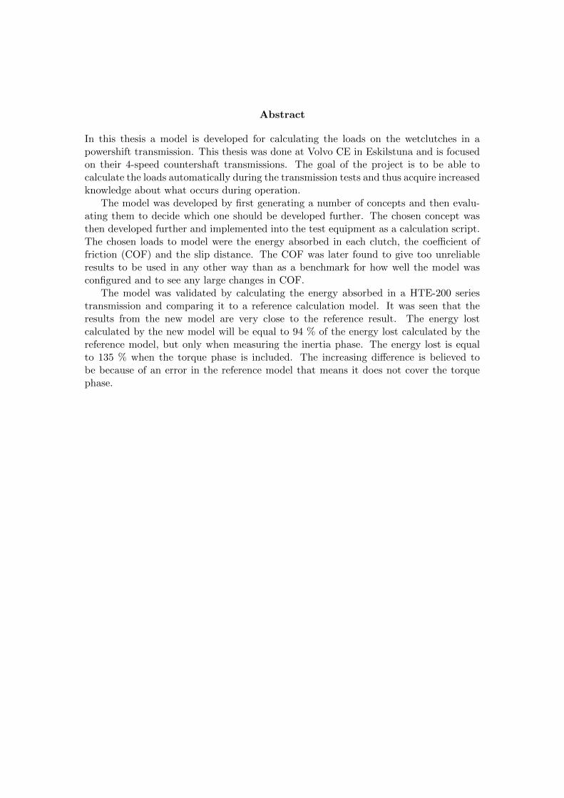
Abstract

In this thesis a model is developed for calculating the loads on the wetclutches in apowershift transmission. This thesis was done at Volvo CE in Eskilstuna and is focusedon their 4-speed countershaft transmissions. The goal of the project is to be able tocalculate the loads automatically during the transmission tests and thus acquire increasedknowledge about what occurs during operation.

The model was developed by first generating a number of concepts and then evalu-ating them to decide which one should be developed further. The chosen concept wasthen developed further and implemented into the test equipment as a calculation script.The chosen loads to model were the energy absorbed in each clutch, the coefficient offriction (COF) and the slip distance. The COF was later found to give too unreliableresults to be used in any other way than as a benchmark for how well the model wasconfigured and to see any large changes in COF.

The model was validated by calculating the energy absorbed in a HTE-200 seriestransmission and comparing it to a reference calculation model. It was seen that theresults from the new model are very close to the reference result. The energy lostcalculated by the new model will be equal to 94 % of the energy lost calculated by thereference model, but only when measuring the inertia phase. The energy lost is equalto 135 % when the torque phase is included. The increasing difference is believed tobe because of an error in the reference model that means it does not cover the torquephase.

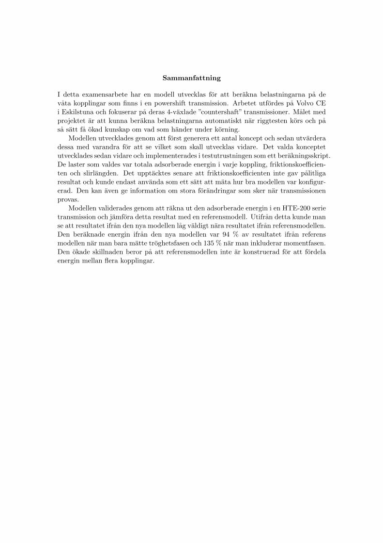
Sammanfattning

I detta examensarbete har en modell utvecklas for att berakna belastningarna pa devata kopplingar som finns i en powershift transmission. Arbetet utfordes pa Volvo CEi Eskilstuna och fokuserar pa deras 4-vaxlade ”countershaft” transmissioner. Malet medprojektet ar att kunna berakna belastningarna automatiskt nar riggtesten kors och pasa satt fa okad kunskap om vad som hander under korning.

Modellen utvecklades genom att forst generera ett antal koncept och sedan utvarderadessa med varandra for att se vilket som skall utvecklas vidare. Det valda konceptetutvecklades sedan vidare och implementerades i testutrustningen som ett berakningsskript.De laster som valdes var totala adsorberade energin i varje koppling, friktionskoefficien-ten och slirlangden. Det upptacktes senare att friktionskoefficienten inte gav palitligaresultat och kunde endast anvanda som ett satt att mata hur bra modellen var konfigur-erad. Den kan aven ge information om stora forandringar som sker nar transmissionenprovas.

Modellen validerades genom att rakna ut den adsorberade energin i en HTE-200 serietransmission och jamfora detta resultat med en referensmodell. Utifran detta kunde manse att resultatet ifran den nya modellen lag valdigt nara resultatet ifran referensmodellen.Den beraknade energin ifran den nya modellen var 94 % av resultatet ifran referensmodellen nar man bara matte troghetsfasen och 135 % nar man inkluderar momentfasen.Den okade skillnaden beror pa att referensmodellen inte ar konstruerad for att fordelaenergin mellan flera kopplingar.

Acknowledgements

I would like to thank everyone at Volvo CE in Eskilstuna who has helped me during thisproject with questions and information. I especially want to thank Joakim Lundin atVolvo who has been a great supervisor and support.

I also want to thank Hans Lofgren at Karlstad University who has also been a greatsupervisor and provided excellent feedback. And I would also like to thank my examinerJens Bergstrom.

And finally a big thanks to everyone else who has helped me with the project.

Filip Gustafsson, Karlstad 9/6/14

Contents

1 Introduction 11.1 Background . . . . . . . . . . . . . . . . . . . . . . . . . . . . . . . . . . . 11.2 Purpose . . . . . . . . . . . . . . . . . . . . . . . . . . . . . . . . . . . . . 11.3 Goals . . . . . . . . . . . . . . . . . . . . . . . . . . . . . . . . . . . . . . 21.4 Delimitations . . . . . . . . . . . . . . . . . . . . . . . . . . . . . . . . . . 2

2 Literature Survey 32.1 Powershift . . . . . . . . . . . . . . . . . . . . . . . . . . . . . . . . . . . . 3

2.1.1 Basic design . . . . . . . . . . . . . . . . . . . . . . . . . . . . . . . 32.1.2 Shifting procedure . . . . . . . . . . . . . . . . . . . . . . . . . . . 4

2.2 Wet clutches . . . . . . . . . . . . . . . . . . . . . . . . . . . . . . . . . . 62.2.1 Heating and cooling of a wet clutch . . . . . . . . . . . . . . . . . 72.2.2 Frictionally-excited thermoelastic instability (TEI) . . . . . . . . . 82.2.3 Wear and degradation of a wet clutch . . . . . . . . . . . . . . . . 82.2.4 Drag torque . . . . . . . . . . . . . . . . . . . . . . . . . . . . . . . 9

2.3 Torque-converter . . . . . . . . . . . . . . . . . . . . . . . . . . . . . . . . 102.4 Lifetime estimation . . . . . . . . . . . . . . . . . . . . . . . . . . . . . . . 10

2.4.1 S-N curve . . . . . . . . . . . . . . . . . . . . . . . . . . . . . . . . 102.4.2 Palmgren-Miner rule . . . . . . . . . . . . . . . . . . . . . . . . . . 11

2.5 Powershift simulations . . . . . . . . . . . . . . . . . . . . . . . . . . . . . 11

3 Method 133.1 Concept generation . . . . . . . . . . . . . . . . . . . . . . . . . . . . . . . 13

3.1.1 Concept 1 . . . . . . . . . . . . . . . . . . . . . . . . . . . . . . . . 133.1.2 Concept 2 . . . . . . . . . . . . . . . . . . . . . . . . . . . . . . . . 133.1.3 Concept 3 . . . . . . . . . . . . . . . . . . . . . . . . . . . . . . . . 14

3.2 Concept elimination . . . . . . . . . . . . . . . . . . . . . . . . . . . . . . 153.3 Detailed development . . . . . . . . . . . . . . . . . . . . . . . . . . . . . 16

3.3.1 Gear reduction and inertia calculations . . . . . . . . . . . . . . . 163.3.2 Power calculation . . . . . . . . . . . . . . . . . . . . . . . . . . . . 17

i

CONTENTS

3.3.3 Energy calculations . . . . . . . . . . . . . . . . . . . . . . . . . . 203.3.4 COF calculations . . . . . . . . . . . . . . . . . . . . . . . . . . . . 203.3.5 Slip distance calculation . . . . . . . . . . . . . . . . . . . . . . . . 20

3.4 Implementation into test equipment . . . . . . . . . . . . . . . . . . . . . 203.4.1 Pre-processing . . . . . . . . . . . . . . . . . . . . . . . . . . . . . 213.4.2 Data recording . . . . . . . . . . . . . . . . . . . . . . . . . . . . . 213.4.3 Main calculation script . . . . . . . . . . . . . . . . . . . . . . . . . 21

3.5 Validation . . . . . . . . . . . . . . . . . . . . . . . . . . . . . . . . . . . . 23

4 Results 254.1 Inertia phase . . . . . . . . . . . . . . . . . . . . . . . . . . . . . . . . . . 254.2 Torque and inertia phase . . . . . . . . . . . . . . . . . . . . . . . . . . . . 26

5 Discussion 275.1 Model assumptions . . . . . . . . . . . . . . . . . . . . . . . . . . . . . . . 27

5.1.1 Friction models . . . . . . . . . . . . . . . . . . . . . . . . . . . . . 275.1.2 Wear of clutches . . . . . . . . . . . . . . . . . . . . . . . . . . . . 275.1.3 Contact states . . . . . . . . . . . . . . . . . . . . . . . . . . . . . 285.1.4 Spring force . . . . . . . . . . . . . . . . . . . . . . . . . . . . . . . 28

5.2 Model integration . . . . . . . . . . . . . . . . . . . . . . . . . . . . . . . . 285.3 Signal quality . . . . . . . . . . . . . . . . . . . . . . . . . . . . . . . . . . 285.4 Validation results . . . . . . . . . . . . . . . . . . . . . . . . . . . . . . . . 295.5 Accuracy of the COF . . . . . . . . . . . . . . . . . . . . . . . . . . . . . . 295.6 Lifetime estimation . . . . . . . . . . . . . . . . . . . . . . . . . . . . . . . 295.7 Further improvements . . . . . . . . . . . . . . . . . . . . . . . . . . . . . 30

6 Conclusions 316.1 Development . . . . . . . . . . . . . . . . . . . . . . . . . . . . . . . . . . 316.2 Verification . . . . . . . . . . . . . . . . . . . . . . . . . . . . . . . . . . . 316.3 Lifetime estimation . . . . . . . . . . . . . . . . . . . . . . . . . . . . . . . 316.4 Further development . . . . . . . . . . . . . . . . . . . . . . . . . . . . . . 31

7 Bibliography 33

Appendices 36

A Concept Comparison Table 37

B Constraint Matrix Examples and Matrix Notations 39B.1 Example constraint equations . . . . . . . . . . . . . . . . . . . . . . . . . 40B.2 Example constraint matrix . . . . . . . . . . . . . . . . . . . . . . . . . . 40B.3 C[:,N] notation . . . . . . . . . . . . . . . . . . . . . . . . . . . . . . . . . 42

ii

CONTENTS

C Power and Friction Calculations 43C.1 Power split . . . . . . . . . . . . . . . . . . . . . . . . . . . . . . . . . . . 44C.2 COF . . . . . . . . . . . . . . . . . . . . . . . . . . . . . . . . . . . . . . . 46

D Calculation Scripts 47D.1 Main calculation script . . . . . . . . . . . . . . . . . . . . . . . . . . . . . 48D.2 Intermediate speed calculations. . . . . . . . . . . . . . . . . . . . . . . . . 49D.3 Rotation direction fix . . . . . . . . . . . . . . . . . . . . . . . . . . . . . 49D.4 COF calculations . . . . . . . . . . . . . . . . . . . . . . . . . . . . . . . . 50

iii

1Introduction

1.1 Background

Volvo Construction Equipment is one of the world’s leading manufacturers of wheelloaders and articulated haulers, with over 14 thousand employees all over the worldand net sales of 64 billion SEK. To maintain this position, constant development of thecompany and its products is needed [1]. One of the developments that Volvo CE focuseson is the drive-trains in their machines to meet the increasing environmental legislationrequirements as well as lowering fuel consumption. This is mainly done at the VolvoTechnical Centre in Eskilstuna.

Today some Volvo machines utilize a powershift transmission, this transmission isbased on a shifting technique that uses wet clutches to shift gears without losing outputtorque [2]. This technique requires great understanding of how wet clutches operatesto get a smooth gear shift with little wear on the components. During development ofa new powershift transmission a lot of tests have to be performed and the current testsetup will yield little information on what actually happens to the wet clutches duringthese tests. This will make it difficult to identify the causes for failure during the test.

1.2 Purpose

The purpose of this project is to create a model that calculates the loads in the clutchesduring testing and presents it in real time as the test is run. This new data can then beused to determine the cause of failure during certain scenarios and then utilized whendesigning new more efficient transmissions as well as investigating failure in existingtransmissions.

1

1.3. GOALS CHAPTER 1. INTRODUCTION

1.3 Goals

The overall goal of this project is to create a model which describes the loads that theclutches are subjected to during test. The project includes:

• Determining appropriate loads to model.

• Creating a model for calculating these loads during testing.

• Validation with existing test data.

• Implementing the model in Volvo test measurement software.

• Investigating how the lifetime and wear can be determined from this model.

1.4 Delimitations

The following delimitations were made on the project:

• The test rig will be unmodified and only the existing hardware will be used.

• The investigation of lifetime and wear will only be a theoretical one and no exper-iments on this will be performed.

• The model will only be run in a test rig and not tested in a real machine.

• If the model is not producing acceptable results it will not be tested in a test rig.

• The model should be simple and fast enough to be calculated while the test isrunning.

• The model will be developed for Volvo’s 4-speed countershaft transmissions forwheel loaders.

• Validation of the model will be against a HTE200 transmission.

2

2Literature Survey

This chapter will provide a theoretical background to the project and explain basicconcepts such as how a powershift works and how it has been modelled previously.

2.1 Powershift

A powershift transmission is a transmission designed to shift gears without interruptingthe transmitted torque. This is done by using wet clutches to switch between active gearratios. [3]

2.1.1 Basic design

A powershift transmission can be designed in many different ways but the commonfeature is that it will have two or more wet clutches mounted in parallel between which toshift the torque. The transmission can also have multiple wet clutch ”gearboxes”mountedin series allowing for additional gear ratios to be achieved. An example transmission canbe seen in figure 2.1. This features two gearboxes in series, two directional gears andfour speed gears. [4, 3]

3

2.1. POWERSHIFT CHAPTER 2. LITERATURE SURVEY

Figure 2.1: Schematic view of a powershift transmission with a separate wet clutch foreach gear.

2.1.2 Shifting procedure

The gear shifting procedure in a powershift transmission is a bit more complicated thanin a regular transmission, There are four different gear shifting scenarios that can occurbut they all share the same shifting phases:

• Filling phase. A flow impulse from the actuation system moves the piston to thekissing point, which is the position where the friction surfaces come into contactwith each other.

• Torque phase. During this phase the torque will be shifted over from the disen-gaging to the engaging clutch.

• Inertia phase. During this phase the speed difference between the plates in thedisengaging clutch will increase while the speed difference in the engaging clutchwill decrease to zero. This is due to internal inertias that is needed to be overcome.

The order of these phases will depend on the shifting scenario. These can be seen intable 2.1. One common factor is that all scenarios will begin with the filling phase.

4

2.1. POWERSHIFT CHAPTER 2. LITERATURE SURVEY

Table 2.1: Phase order in different shifting scenarios.

With positive input torque With negative input torque

(driving) (braking)

Upshift Torque phase → Inertia phase Inertia phase → Torque phase

Downshift Inertia phase → Torque phase Torque phase → Inertia phase

To better explain how a gear shift in a powershift transmission is carried out one canconsider a scenario were a person on skis is going uphill between two ropes. The ropesare moving at different speeds and the person is holding on to the slower rope as shownin step 1 in figure 2.2. In order to change speed to the same as the fast rope the personhas to perform the following steps:

1. The person is starting out travelling at the same speed as the slow rope.

2. The person then grabs the faster rope with increasing pressure thus decreasing thepull force in the slow rope hand and increasing it in the fast rope hand.

3. At this point the pull force in the hand with the slow rope equal is to zero.

4. The slow rope is now released and the pressure in the fast rope hand is increasedto accelerate the person.

5. The person is now travelling at the same speed as the fast rope.

Figure 2.2: An illustration showing a man going up a hill changing speed in a way equiv-alent to a powershift.

This scenario is equivalent to an upshift with positive torque. The other shift scenarioswill be performed in a similar way but in a different order, as shown in table 2.1.[2]

The pressure levels and slipspeeds for an upshift with positive torque can be seen infigure 2.3.

5

2.2. WET CLUTCHES CHAPTER 2. LITERATURE SURVEY

Figure 2.3: Illustration of the pressure and slipspeeds occurring in a shift from third (F3)to fourth (F4) forward gear.

2.2 Wet clutches

Wet clutches are a type of friction clutch that is constantly lubricated to reduce wear andincrease the cooling capacity. This makes is possible for the clutch to operate at higherloads than a regular clutch. These types of clutch are used in many applications suchas automatic transmissions in cars and also in torque converters as lock-up clutches anddifferent locking devices. A schematic drawing of a wet clutch can be seen in figure 2.4.[5]

Figure 2.4: Schematic view of the components in a wet clutch. [6]

These kinds of clutches are usually engaged using a hydraulic piston. To engagethe clutch a pressure is applied to the piston. This moves the plates closer together andcreates the friction force needed to transfer the torque. A return spring is mounted insidethe clutch to push back the piston and disengage the clutch when the piston pressureis decreased. This process of engaging the clutch can be divided into four stages: fullydisengaged, filling, engagement and fully engaged. [5]

6

2.2. WET CLUTCHES CHAPTER 2. LITERATURE SURVEY

The friction discs in a wet clutch are often made of a steel core with a paper-basedfriction material on both sides. This paper-based friction material has grooves in it togive the oil trapped between the plates a way to escape as well as provide a flow of oilfor cooling when engaged. Figure 2.5 shows a friction disc with grooves.[7]

The wet clutch exhibit torque loss due to shear forces caused by the oil. This is calleddrag torque. In Section 2.2.4 the concept of drag torque will be further described.

Figure 2.5: Drawing of a friction disc for use in a wet clutch. [7]

2.2.1 Heating and cooling of a wet clutch

Friction heating

When two surfaces slide against each other heat is generated. This happens during theworking mode for a wet clutch in normal operation. In some cases ”hotspots” will formon the disc due to this kind of heating. This is described in more detail in Section 2.2.2.

The power generated by sliding can be calculated using equation 2.1 were Pavg is thegenerated power, T is the transferred torque and ω1 and ω2 are the the angular velocityof the friction disc and mating plate. [8]

Pavg = T ∗ |(ω1 − ω2)| (2.1)

Cooling of the wet clutch

The primary cooling mechanism in a wet clutch during operation is heat transfer to theoil. The effect of the cooling can be varied by for example altering the flow rate or thegeometry of the friction disc grooves. [8]

7

2.2. WET CLUTCHES CHAPTER 2. LITERATURE SURVEY

2.2.2 Frictionally-excited thermoelastic instability (TEI)

The formation of hot spots is a common problem in clutches. These are formed dueto high localized temperature and pressure zones. These localized temperature zonesare created due to non-uniformity in the contact pressure distribution across the sur-face. Areas that experience higher pressure will also experience higher temperature. Thepressure will then increase in the area as the temperature rises due to localized thermalexpansion thus increasing the temperature further. This is called thermoelastic instabil-ity (TEI), but is normally referred to as ”hot spots”. The material in these zones willeffectively be heat-treated, and for example a martensite structure can be created in theferrous materials. An example of a steel separator disc with hot spots can be seen infigure 2.6.[9]

Figure 2.6: Steel separator disc with hot spots.[9]

The types of hotspots can be divided into two main groups: focal hotspots and bandhotspots. Focal hotspots are hotspots that are discontinuous in the sliding direction thusforming distributed spots around the disk. Band hotspots are continuous bands whichgo around the friction surface forming concentric circles. It has been shown that themost common case when dealing with two dissimilar materials is focal hot spots.[9]

2.2.3 Wear and degradation of a wet clutch

The discs in a wet clutch will be subjected to wear during its lifetime and thus some ofits properties will change. These properties includes the friction coefficient, real contactarea and width of the plate. Tests done on wet clutch wear have shown that the wearrate will be severe in the fist 200 cycles with noticeable change in thickness and thenlowered after this run-in period. It has also been seen that the friction plates closest tothe piston will suffer the most from this wear. [10]

If the temperature gets too high during operation it may cause the cellulose to de-compose leading to degradation of the friction material. This usually happens around200 to 400 ◦C [10]. Another failure mode that can occur during operation is glazing ofthe friction material. This is caused by deposition of fluid degradation products on the

8

2.2. WET CLUTCHES CHAPTER 2. LITERATURE SURVEY

surface creating a darkened smooth or shiny surface. The glazing often causes a decreasein friction and sometimes increases the friction in the boundary regime [10].

2.2.4 Drag torque

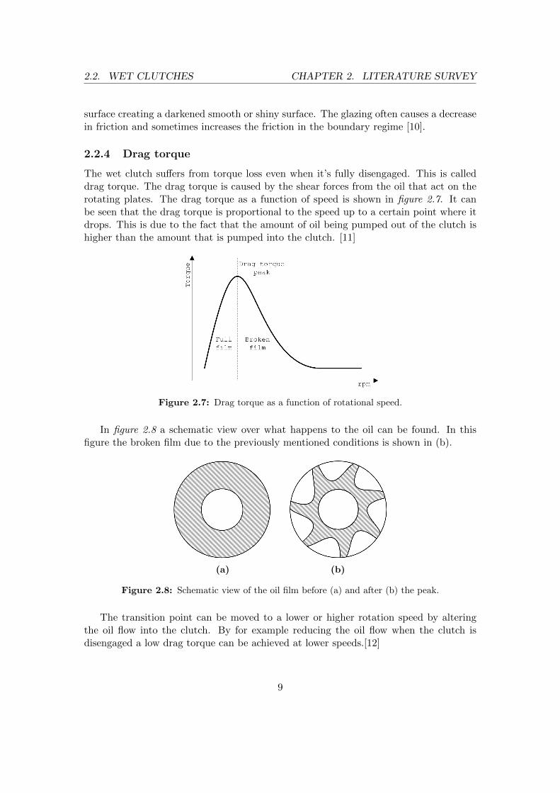
The wet clutch suffers from torque loss even when it’s fully disengaged. This is calleddrag torque. The drag torque is caused by the shear forces from the oil that act on therotating plates. The drag torque as a function of speed is shown in figure 2.7. It canbe seen that the drag torque is proportional to the speed up to a certain point where itdrops. This is due to the fact that the amount of oil being pumped out of the clutch ishigher than the amount that is pumped into the clutch. [11]

Figure 2.7: Drag torque as a function of rotational speed.

In figure 2.8 a schematic view over what happens to the oil can be found. In thisfigure the broken film due to the previously mentioned conditions is shown in (b).

(a) (b)

Figure 2.8: Schematic view of the oil film before (a) and after (b) the peak.

The transition point can be moved to a lower or higher rotation speed by alteringthe oil flow into the clutch. By for example reducing the oil flow when the clutch isdisengaged a low drag torque can be achieved at lower speeds.[12]

9

2.3. TORQUE-CONVERTER CHAPTER 2. LITERATURE SURVEY

2.3 Torque-converter

A torque converter is a device that uses hydrodynamic forces to transfer power in aflexible way. These are often used to replace the clutch between the engine and thetransmission in automatic transmission.

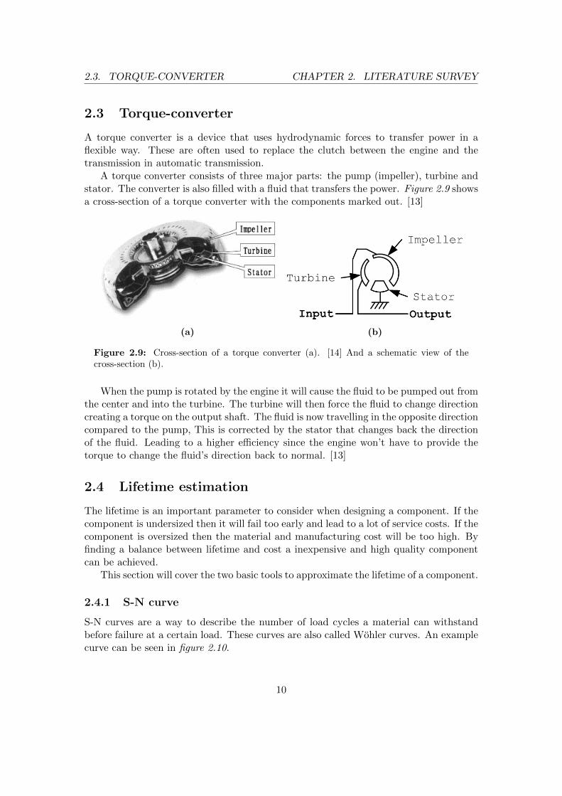
A torque converter consists of three major parts: the pump (impeller), turbine andstator. The converter is also filled with a fluid that transfers the power. Figure 2.9 showsa cross-section of a torque converter with the components marked out. [13]

(a) (b)

Figure 2.9: Cross-section of a torque converter (a). [14] And a schematic view of thecross-section (b).

When the pump is rotated by the engine it will cause the fluid to be pumped out fromthe center and into the turbine. The turbine will then force the fluid to change directioncreating a torque on the output shaft. The fluid is now travelling in the opposite directioncompared to the pump, This is corrected by the stator that changes back the directionof the fluid. Leading to a higher efficiency since the engine won’t have to provide thetorque to change the fluid’s direction back to normal. [13]

2.4 Lifetime estimation

The lifetime is an important parameter to consider when designing a component. If thecomponent is undersized then it will fail too early and lead to a lot of service costs. If thecomponent is oversized then the material and manufacturing cost will be too high. Byfinding a balance between lifetime and cost a inexpensive and high quality componentcan be achieved.

This section will cover the two basic tools to approximate the lifetime of a component.

2.4.1 S-N curve

S-N curves are a way to describe the number of load cycles a material can withstandbefore failure at a certain load. These curves are also called Wohler curves. An examplecurve can be seen in figure 2.10.

10

2.5. POWERSHIFT SIMULATIONS CHAPTER 2. LITERATURE SURVEY

Figure 2.10: En example S-N curve obtained from ultrasonic fatigue tests. [15]

This curve and the Palmgren-Miner rule provide a powerful tool for calculating thelifetime of a component.

2.4.2 Palmgren-Miner rule

One theory to calculate the accumulated damage for an item is to use the Palmgren-Miner rule. This rule will specify how much of the items lifetime is spent on each loadcase. When the summarized damage accompanied with each individual load equals to 1failure occurs. This is described in the following equation:∑

i=1

niNi

= 1 (2.2)

were ni is the number of cycles of the current load and Ni is the total number of cyclesto failure with the current load. [16]

2.5 Powershift simulations

There are many ways to simulate a powerhift transmission but one of the more commonis to model the transmission with a lumped element model. This model consists ofsimplified elements that represent different components. This makes it easy to buildcomplex systems that are easy to understand and modify. These models can be builtin programs such as MatLab/Simulink. In figure 2.11 a 4- and 15-degrees of freedom(DOF) model can be seen. [17]

11

2.5. POWERSHIFT SIMULATIONS CHAPTER 2. LITERATURE SURVEY

(a) (b)

Figure 2.11: Lumped element models of a dual clutch transmission. (a) 15 DOF, (b) 4DOF. [17]

By reducing the degrees of freedom a faster calculation time can be achived but sincethe components are simplified it can cause an error in the final results. The models witha higher number of DOF often include a better representation of the stiffness and inertiafor the components.[17]

12

3Method

The following steps were performed to create a working model for calculating the clutchloads: concept generation, concept elimination, further development of the chosen con-cept, implementation into test equipment and validation of result.

3.1 Concept generation

Three major concepts were generated during the investigation and they are presented inthe following sections.

3.1.1 Concept 1

This concept is based on calculating the torque transferred in each clutch by comparingthe input and output torque and taking into account the active gear ratios to the differentclutches. The losses in the transmission are also needed to get the correct torque in eachclutch since some of the torque is lost due to other factors.

3.1.2 Concept 2

This is a simple concept based on calculating the lost energy with a known coefficient offriction. This calculation is made for all the clutches during a shift since the calculationsare independent from each other. The power can be calculated by using the followingequation:

PL = µ ∗ F ∗N ∗ |ω1 − ω2| ∗Ro∫

Ri

dr (3.1)

where µ is the coefficient of friction, N is the number of friction interfaces and the otherconstants (Ri, Ro, F , ω1 and ω2) are described in figure 3.1.

13

3.1. CONCEPT GENERATION CHAPTER 3. METHOD

Figure 3.1: Cross-section of a clutch showing the constants used in Equation 3.1.

3.1.3 Concept 3

This concept is based on calculating the total power lost in the transmission by comparingthe difference in input and output power. The losses in the clutches are then isolated byremoving those due to other factors (drag torque etc.) from the total power loss. Thetransmission will be modelled as a series of clutches and flywheels to calculate the lossesmore easily and to divide the power. This seen in the figure below.

Figure 3.2: Schematic over the different components in the model and how they areconnected.

For each moment in time the power loss in the clutches is divided proportionally tothe theoretical amount of power loss in each clutch. This powersplit is illustrated infigure 3.3 were the angle k of the line is determined by the theoretical power losses Pt.The measured power losses Pm is determined by finding the point on the line were thesum of the two losses is equal to the total power loss Ptot in the clutches.

14

3.2. CONCEPT ELIMINATION CHAPTER 3. METHOD

Figure 3.3: Illustration of how the power is split proportionally to the theoretical power.Ptot is the total power loss, Pt is the theoretical power loss and Pm the measured power loss.

The power loss will first be divided between the two clutch pairs and then betweenthe clutches in each pair.

3.2 Concept elimination

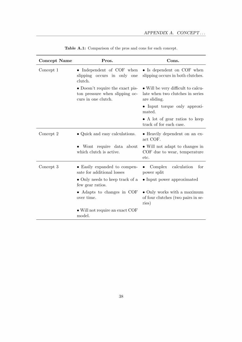
The pros and cons of each concept will be compared to determine which concept willbe developed further. The complete comparison table can be found in appendix A. Asummary of the most important points for each concept is listed in table 3.1. Theexpandability and low dependency on COF is the most important property for thisapplication.

Table 3.1: Comparison between the pros and cons for each concept.

Concept Name Pros. Cons.

Concept 1 • Independent of COF whenslipping occurs in only oneclutch.

• Dependent on COF when slip-ping occurs in both clutches.

Concept 2 • Won’t require data aboutwhich clutch is active.

• Heavily dependent on an ex-act COF.

Concept 3 • Easily expanded to compen-sate for additional losses

• Complex calculation forpower split

•Will not require an exact COFmodel.

• Only works with a maximumof four clutches (two pairs in se-ries)

From this comparison it was decided that concept three is going to be developed

15

3.3. DETAILED DEVELOPMENT CHAPTER 3. METHOD

further mostly due to the fact that it will not be as dependent on how precise thecoefficient of friction is and the fact that it can be easily expanded.

3.3 Detailed development

Concept three will be developed and described in more detail. This section will coverhow the gear ratios, moment of inertia, power, energy, COF and sliding distance arecalculated.

3.3.1 Gear reduction and inertia calculations

The gear ratios and reduced moment of inertia are calculated by using a model describedby David Berggren [18]. This model utilizes matrix calculations to describe the trans-mission and thus becomes very flexible due to the fact that the different designs arecalculated in the same way. The constraints of the transmission will be described by thematrix C which is defined so that equation 3.2 is valid. Some examples of this matrixcan be found in appendix B.

C ∗ ω =

c11 · · · c1n...

. . ....

cm1 · · · cmn

∗ω1...

ωn

= 0 (3.2)

where ω is the angular velocity, m the number of constraints and n is the number ofshafts in the transmission. Each shaft is indexed with a number from one to n. Theshafts are then divided into sensor and other shafts. The ”sensor” shafts are set to bethose with a speed sensor on them and the rest are set to ”other”. The indexes for thesensor shafts are defined in the vector NS.shaft in the order shown in equation 3.3 andthe indexes for the other shafts are defined in the vector NO.shaft.

NS.shaft =[nturb. ninter. noutp.

](3.3)

The gear ratio between the sensor shafts and the other shafts (RO.shaft) can be calculatedusing equation 3.4. An explanation for the C[: ,N ] notation can be found in appendix B.

RO.shaft = −C[: ,NO.shaft]−1 ∗C[: ,NS.shaft] (3.4)

The gear ratio between the sensor shafts (RS.shafts) is given by an n×n identity matrixwere n is the number of sensor shafts as shown in equation 3.5. This is due to the factthat for simplicity’s sake all the clutches are defined as open and their shafts independentof each other.

RS.shaft = I =

1 0 · · ·0 1 · · ·...

.... . .

(3.5)

16

3.3. DETAILED DEVELOPMENT CHAPTER 3. METHOD

The equivalent moment of inertia is calculated by the following steps: first the momentof inertia for each shaft is defined in the vector J as shown in the following equation:

J =[J1 J2 · · · Jn

]T(3.6)

These are then divided into two vectors one for other shafts (JO.shaft) and one for sensorshafts (JS.shaft).

JS.shaft = J [NS.shaft] (3.7)

JO.shaft = J [NO.shaft] (3.8)

By using equation 3.9 the equivalent moment of inertia at each sensor shaft is calculated.

Jequ = diag(JS.shaft) + RTO.shaft ∗ diag(JO.shaft) ∗RO.shaft (3.9)

The results this equation will have the form:

Jequ =

Jturb. 0 0

0 Jinter. 0

0 0 Joutp.

(3.10)

3.3.2 Power calculation

The power lost in the clutches will be estimated by first calculating the total power lostin the transmission and then removing the power gained or lost by inertia as well as thepower lost due to other effects such as drag torque. This is described by the followingequation:

Pall cl. = |Pin − Put|︸ ︷︷ ︸Total loss

−∑

(Pinertia,i)︸ ︷︷ ︸Loss/gain due to inertia

− Pmisc.︸ ︷︷ ︸Other losses

(3.11)

The input and output power can be calculated using the torque and angular velocity asper:

P = T ∗ ω (3.12)

were P is the power, T is the torque and ω is the angular velocity. The following equationcan be used to calculate the power lost or gained due to inertia.

Pinertia,i =d

dt(1

2∗ Ji ∗ ω2

i ) (3.13)

where J is the moment of inertia and ω is the angular velocity of the shaft.The active mode of each clutch needs to be determined in order to decide how to

split the power between the clutches. This is done by observing the clamp force (Fc) andslip speed (|∆ω|). Table 3.2 describes which mode is active at different conditions. Thesync mode is when the clutch plates are in contact and no slip occurs, the open mode iswhen the clutch plates are not in contact. The working mode is when the clutch plates

17

3.3. DETAILED DEVELOPMENT CHAPTER 3. METHOD

are in contact and there is a slip between the plates, the clutch will experience frictionalheating during this mode.

Table 3.2: Table describing which mode is active in different conditions.

Fc ≤ 0 Fc > 0

|∆ω| = 0 - Sync (S)

|∆ω| > 0 Open (O) Working Mode (W)

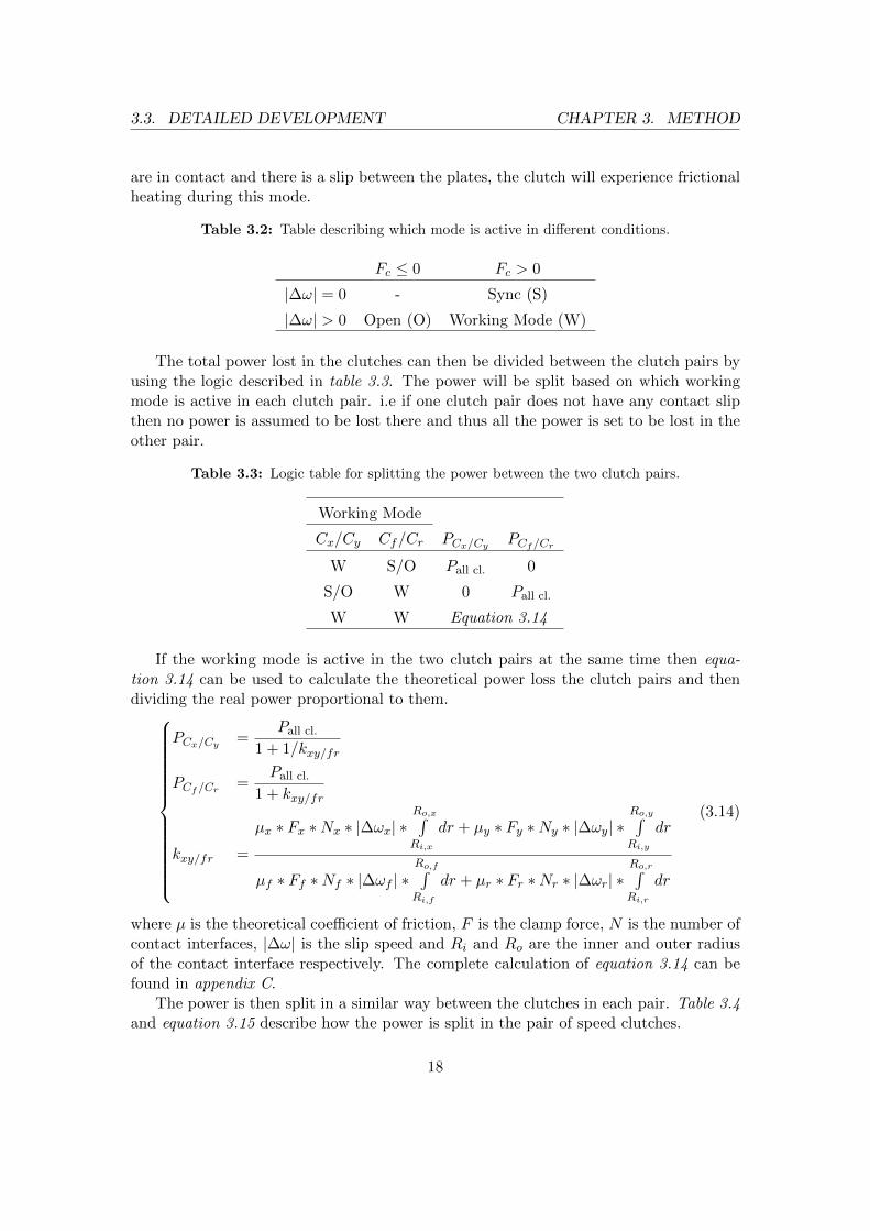
The total power lost in the clutches can then be divided between the clutch pairs byusing the logic described in table 3.3. The power will be split based on which workingmode is active in each clutch pair. i.e if one clutch pair does not have any contact slipthen no power is assumed to be lost there and thus all the power is set to be lost in theother pair.

Table 3.3: Logic table for splitting the power between the two clutch pairs.

Working Mode

Cx/Cy Cf/Cr PCx/CyPCf/Cr

W S/O Pall cl. 0

S/O W 0 Pall cl.

W W Equation 3.14

If the working mode is active in the two clutch pairs at the same time then equa-tion 3.14 can be used to calculate the theoretical power loss the clutch pairs and thendividing the real power proportional to them.

PCx/Cy=

Pall cl.

1 + 1/kxy/fr

PCf/Cr=

Pall cl.

1 + kxy/fr

kxy/fr =

µx ∗ Fx ∗Nx ∗ |∆ωx| ∗Ro,x∫Ri,x

dr + µy ∗ Fy ∗Ny ∗ |∆ωy| ∗Ro,y∫Ri,y

dr

µf ∗ Ff ∗Nf ∗ |∆ωf | ∗Ro,f∫Ri,f

dr + µr ∗ Fr ∗Nr ∗ |∆ωr| ∗Ro,r∫Ri,r

dr

(3.14)

where µ is the theoretical coefficient of friction, F is the clamp force, N is the number ofcontact interfaces, |∆ω| is the slip speed and Ri and Ro are the inner and outer radiusof the contact interface respectively. The complete calculation of equation 3.14 can befound in appendix C.

The power is then split in a similar way between the clutches in each pair. Table 3.4and equation 3.15 describe how the power is split in the pair of speed clutches.

18

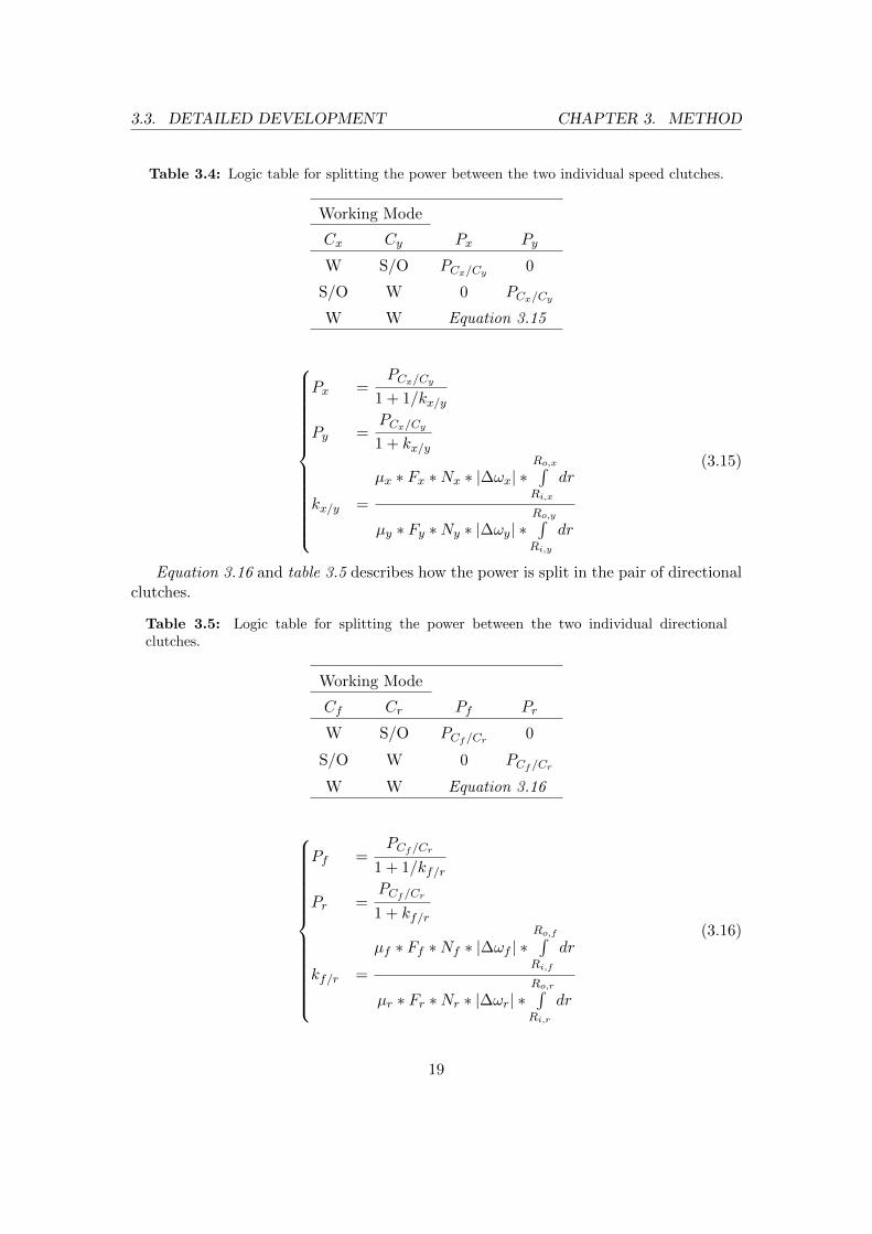
3.3. DETAILED DEVELOPMENT CHAPTER 3. METHOD

Table 3.4: Logic table for splitting the power between the two individual speed clutches.

Working Mode

Cx Cy Px Py

W S/O PCx/Cy0

S/O W 0 PCx/Cy

W W Equation 3.15

Px =PCx/Cy

1 + 1/kx/y

Py =PCx/Cy

1 + kx/y

kx/y =

µx ∗ Fx ∗Nx ∗ |∆ωx| ∗Ro,x∫Ri,x

dr

µy ∗ Fy ∗Ny ∗ |∆ωy| ∗Ro,y∫Ri,y

dr

(3.15)

Equation 3.16 and table 3.5 describes how the power is split in the pair of directionalclutches.

Table 3.5: Logic table for splitting the power between the two individual directionalclutches.

Working Mode

Cf Cr Pf Pr

W S/O PCf/Cr0

S/O W 0 PCf/Cr

W W Equation 3.16

Pf =PCf/Cr

1 + 1/kf/r

Pr =PCf/Cr

1 + kf/r

kf/r =

µf ∗ Ff ∗Nf ∗ |∆ωf | ∗Ro,f∫Ri,f

dr

µr ∗ Fr ∗Nr ∗ |∆ωr| ∗Ro,r∫Ri,r

dr

(3.16)

19

3.4. IMPLEMENTATION INTO TEST . . . CHAPTER 3. METHOD

The complete calculations for these equations can be found in appendix C.The theoretical coefficient of friction used to split the power between the clutches

can be modelled in many ways. For example, constant or linear dependent on slip speed.When assuming it is constant then the power split will become independent of the COF.

3.3.3 Energy calculations

The total energy lost in each clutch is calculated by integrating the power over time foreach clutch as seen in equation 3.17, where Ec is the total energy loss of a the clutchand Pc(t) is the power loss of the clutch as a function of time.

Ec =

∫Pc(t) dt (3.17)

3.3.4 COF calculations

The coefficient of friction can be calculated by comparing the results from the powercalculations with the theoretical power lost as seen in the following equation.

µ =Pmodel

F ∗N ∗ |∆ω| ∗Ro∫Ri

dr

(3.18)

where Pmodel is the calculated power lost in the clutch, F is the clamping force, N is thenumber of friction interfaces, |∆ω| is the absolute sliding speed and Ri and Ro are theinner and outer radius of the contact interface respectively. The full calculation can befound in appendix C.

3.3.5 Slip distance calculation

The slip distance is calculated by calculating the distance a point at the mean radiusof the disc has travelled during the the working and sync mode of a shift. This can bedone with the following equation:

Sslip = rmean ∗ 2π ∗∫|∆ω|dt (3.19)

where Sslip is the slip distance, rmean is the mean radius of the disc and |∆ω| is the slipspeed.

3.4 Implementation into test equipment

A script has been written to carry out the calculations during tests. The main script isprogrammed in a calculation program called ”imc FAMOS” but some supporting scriptsare made in MatLab due to the large amount of matrix operations.

The script can be divided into three parts: pre-processing, data recording and maincalculations.

20

3.4. IMPLEMENTATION INTO TEST . . . CHAPTER 3. METHOD

• The pre-processing is carried out before the test is started and contains all thecalculations that don’t change during the test such as those for inertia and gearratio.

• The data recording part will record sensor data from the test rig and save it sothat the main script can process it.

• The main calculations will process the recorded data and calculate the energiesand COF.

The following sections will describe each part in more detail.

3.4.1 Pre-processing

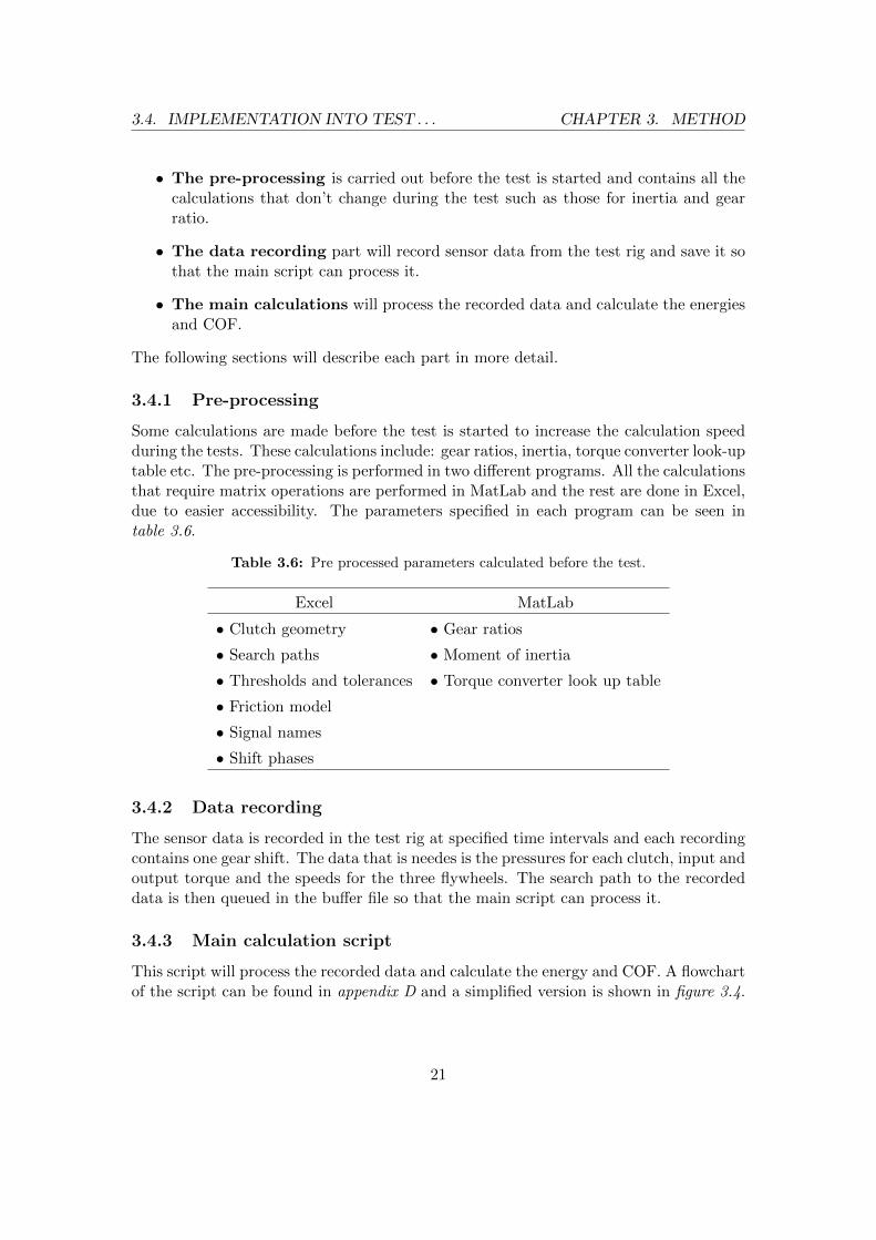
Some calculations are made before the test is started to increase the calculation speedduring the tests. These calculations include: gear ratios, inertia, torque converter look-uptable etc. The pre-processing is performed in two different programs. All the calculationsthat require matrix operations are performed in MatLab and the rest are done in Excel,due to easier accessibility. The parameters specified in each program can be seen intable 3.6.

Table 3.6: Pre processed parameters calculated before the test.

Excel MatLab

• Clutch geometry • Gear ratios

• Search paths • Moment of inertia

• Thresholds and tolerances • Torque converter look up table

• Friction model

• Signal names

• Shift phases

3.4.2 Data recording

The sensor data is recorded in the test rig at specified time intervals and each recordingcontains one gear shift. The data that is needes is the pressures for each clutch, input andoutput torque and the speeds for the three flywheels. The search path to the recordeddata is then queued in the buffer file so that the main script can process it.

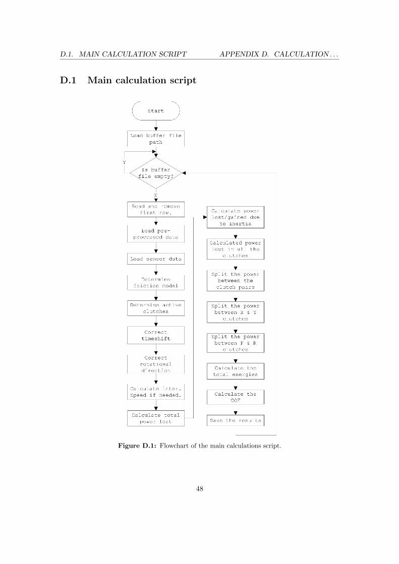
3.4.3 Main calculation script

This script will process the recorded data and calculate the energy and COF. A flowchartof the script can be found in appendix D and a simplified version is shown in figure 3.4.

21

3.4. IMPLEMENTATION INTO TEST . . . CHAPTER 3. METHOD

Figure 3.4: Simplified flowchart of the main calculations script.

The following sections will describe the different steps carried out by the main cal-culation script.

Check for new sensor data

The script will check if the buffer file contains any search paths. If it does then it willprocess the buffered data and remove the search path from the file. If no paths existsthen the script will wait for a specified time and then try again.

Load pre-processed data

The script will load all the pre-processed data at the beginning of the calculations toensure that the most up to date data is loaded in case some minor adjustments areperformed during the tests.

Load sensor data

The script will load all the raw sensor data from the file path fetched from the bufferfile. The names of the sensor channels loaded are defined in the excel file.

In case the intermediate speed sensor channel is missing then the speeds will becalculated from the other sensors. This creates a new limitation where both clutch pairscannot be active at the same time. The algorithm for this can be found in appendix D.

Pre-process recorded data

Pre-processing of the recorded data is needed before the energies and COF can be cal-culated. This includes determining which clutches are active, adjusting the time shiftand correcting the rotational directions.

The active clutches are determined by checking if the pressure in each clutch changesfrom max to min or min to max. If this is the case then the clutch is assumed to beactive. If the number of active clutches exceeds four then the calculations will be abortedsince the model is not compatible with more than two clutch pairs.

In order to use sensor data from different sources they need to be synchronized.This is achieved by comparing the same sensor signal from the different sources andcalculating the time-shift by using built-in functions in FAMOS.

22

3.5. VALIDATION CHAPTER 3. METHOD

The duration of each phase is also measured from the ECU output. The slip distancefor each clutch is also calculated, as described in section 3.3.

The final operation is to correct the rotational direction of the measured absoluterotational speed. This is done by a script that looks for points where change in rotationaldirection should occur and uses these to modify the speed signals. More information onhow this is done can be found in appendix D.

Calculate energies and COF

The energies and COF are calculated by using the method described in section 3.3. Amore detailed description can be found in appendix D.

Save the results

The results of the calculations are saved in comma separated text files and each timethe script is run it will append the new result at the end of the file.

3.5 Validation

The model is validated by comparing the results with those from an existing referencemodel for calculating the energy. The reference model calculates the energy by utilizingthe known gear ratio for a chosen clutch along with the output torque to determine thetransferred torque at that clutch. The efficiency of the gears between the clutch and theoutput shaft is also considered. This can be seen in the following equation:

Tc =Tout ∗R

η(3.20)

where Tc is the clutch torque, Tout is the the output torque, η is the efficiency and R isthe gear ratio between the output and the clutch. The power lost in the clutch can thenbe calculated with the following equation:

Pc = Tc ∗∆ω (3.21)

where ∆ω is the slip speed and Pc is the power lost in the clutch. The total energy isthen calculated the same way as in the new model as seen in equation 3.17. A limitationto this reference model is that it’s only valid during the inertia phase and thus the powerin the other phases is set to zero.

The analysed gearshift is a shift from third (F3) to fourth (F4) forward gear. Calcu-lations are made on a full shift (torque and inertia phase) and just on the inertia phasesince this allows for only one clutch to be experiencing slipping contact. The phases areillustrated in figure 2.3. Several measurements will be analysed to get a mean value forthe difference between the two models.

23

3.5. VALIDATION CHAPTER 3. METHOD

The resulting data will be normalized with mean values for the results from thereference model as seen in the following equation:Enew,norm = Enew/Eref

Eref,norm = Eref/Eref

(3.22)

where Enew and Eref are the results from the new/reference model. Enew,norm andEref,norm are the normalized results from the new/reference model. Eref is the meanresult from the reference model.

24

4Results

The results from the validation tests will be presented in the following two sections. Thefirst section will cover the results from the test data that only contains an inertia phaseand the second section will cover a complete measurement that includes both a torquephase and an inertia phase.

4.1 Inertia phase

The resulting normalized energies from the calclulations of the inertia phase measure-ments can be seen in figure 4.1. Each point represents one shift from F3 to F4.

Figure 4.1: Results from the energy calculation with the new model and the referencemodel. The calculations are made only on the inertia phase.

25

4.2. TORQUE AND INERTIA PHASE CHAPTER 4. RESULTS

The mean energy calculated by the new model on this series of measurements isabout 94% of the mean energy calculated by the reference model.

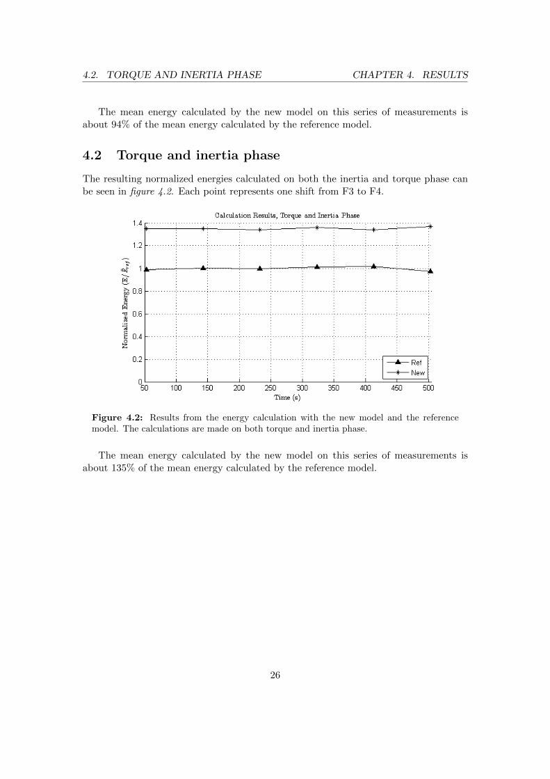
4.2 Torque and inertia phase

The resulting normalized energies calculated on both the inertia and torque phase canbe seen in figure 4.2. Each point represents one shift from F3 to F4.

Figure 4.2: Results from the energy calculation with the new model and the referencemodel. The calculations are made on both torque and inertia phase.

The mean energy calculated by the new model on this series of measurements isabout 135% of the mean energy calculated by the reference model.

26

5Discussion

5.1 Model assumptions

A number of assumptions are made in the model that need to be discussed. Theseinclude wear of the clutches, contact states, spring force, etc.

5.1.1 Friction models

Friction is modelled either as a constant value independent of slip speed or as a linearfunction of the slip speed. The following models were chosen due to two reasons:

• The constant model was chosen since it would allow the model to be independentof the COF thus allowing the script to run even when the COF is not known. Themodel becomes independent due to the fact that the COF for each clutch cancelout one another when calculating the split ratio k. This is the only occasion werethe COF is used.

• The linear model was chosen due to the fact that it would allow for the model torun with a clutch that has a COF which changes a lot when the slip speed changes.

Additional models can be developed if required to get a better representation of how thefriction changes with different conditions, for example the temperature of the clutch.

5.1.2 Wear of clutches

In this model the assumption is made that all clutches wear by the same amount atany given time. This is assumed in this way to make it easier to split the power. Thisassumption is considered valid since wear on the clutches after the run-in period is lowand thus the error created will not be very high compared to errors created by otherfactors.

27

5.2. MODEL INTEGRATION CHAPTER 5. DISCUSSION

This assumption can lead to an error when replacing one clutch and not the otherssince the new clutch will not have gone through the run-in period and will probablyexperience a different coefficient of friction from the rest of the clutches. This will createan error when dividing the power loss between the clutches since the model will not takethe new COF into consideration. This can be corrected by developing a new frictionmodel that takes lifetime into consideration.

This type of problem can also occur when one clutch is subjected to more wear thanthe rest of the clutches.

5.1.3 Contact states

In the current model it is assumed that there is no travel time between when the clampforce is larger than zero and the kissing point where the plates touch. This assumptionis due to the lack of position feedback from the plates and results in a longer slidingworking time than in reality. This may cause a significant problem if the travel time isvery long thus creating an unwanted power split. This may be filtered away by usingfeedback from the ECU or by installing a position sensor for each clutch. Another way isto try and identify certain signatures in the pressure signal that indicate contact betweenthe plates thus making it possible to tell if the travel time is over or not.

5.1.4 Spring force

This model contains an assumption that the spring force is constant and independentof the compression. This is due to the lack of positional feedback for the clutch plates.However since the spring force is only used when dividing the power between the clutchesone can consider this assumption valid.

If an position sensor would be installed in the clutches then the spring force shouldbe modelled as a function of the compression distance to get a better representation ofhow big the clamp force actually is and thus dividing the power more accurately.

5.2 Model integration

The current integration with the test equipment utilizes many different applicationsmaking it very prone to bugs and crashes since there is very little feedback betweenthe programs and it is very hard to achieve a good error handler. This can be solvedby porting the model over to a single program or create a new program that is specificfor this application. This program could also include a configuration wizard to increaseusability of the program and make it easier to get a correct configuration.

5.3 Signal quality

The data is quite heavily filtered when collected by the sensors and this may cause acouple of problems such as incorrect acceleration and loss of important spikes. If the

28

5.4. VALIDATION RESULTS CHAPTER 5. DISCUSSION

acceleration is filtered to an inaccurate value then the power loss/gain in the lumpedinertia elements is going to be incorrect and lead to an error in the total energy loss inthe clutches. If on the other hand a filter is applied to smooth out the curve one couldloose important max and min values. For example the min value where the absoluterotation speed should change direction can be moved upwards thus making it harder forthe program to identify it.

5.4 Validation results

Results from the validation test show that the new model gives a result that lies veryclose to the results from the validation model when only considering the inertia phase.The results differ quite a bit when including the torque phase. This is mainly caused bythe reference model not being able to calculate the power loss during the torque phase.This limitation comes from the fact that during the torque phase there will be morethan one clutch active at the same time and the reference model has no way to splitthe torque between the active clutches. This result do on the other hand show that thetorque phase does matter to the end result and that it is important to consider this whendesigning the clutches.

5.5 Accuracy of the COF

The calculated COF value for each clutch will differ quite a lot from reality since it isheavily dependent on how well all the other losses are modelled. If the losses are forexample modelled to be lower than in reality then the loss in the clutches will be higherand the COF will increase. It should be noted that the calculated COF can still beused as a measurement on how well all the parameters are tuned in the model. If, forexample, a resulting COF of 20 or 100 occurs then one should consider checking if thetest parameters are correct. On the other hand if a COF below one is calculated thenthe model is probably quite well tuned.

The normalized COF can also be used to check for changes over time by comparingit at different run-times. This may be useful for understanding how the clutch wears.

5.6 Lifetime estimation

Approximation of the transmission lifetime could be calculated using the Palmgren-Minerrule combined with an S-N diagram containing the lifetime for a given total energy orshape of the power curve. One problem with this approach is that it will require alarge amount of test data to create the S-N diagram. This can possibly be solved byutilizing existing machines and logging the energy values when they are used by thecostumers, then collecting it during service of the machine. The problem with this isthat one machine is subjected to a lot of different load cases during it’s lifetime so one

29

5.7. FURTHER IMPROVEMENTS CHAPTER 5. DISCUSSION

should consider utilizing some statistical theory to combine the measurements from allthe machines.

One can argue if the shape of the power curve will have a significant impact on theresulting lifetime or if the total energy gives a good enough representation. One thingto consider is that if we have a large power spike then it may lead to problems such ashot spots since the plates are being heated over a very short period of time.

Another approach is to compare the sliding distance for each shift and compare thisto a model that describes the wear as a function of this distance,such as the Archardequation.

5.7 Further improvements

As mentioned previously there are some points where further improvements have beenidentified. These include modelling of drag losses, better data handling and filtering andfriction models.

One area that needs improvement is the modelling of drag losses in the transmission.Since the model is based on the total amount of losses it is important to try and modelall the significant losses correctly. These losses can either be modelled as a constant or asa dynamic function that varies depending on some parameters. The second alternativewill probably provide a better result that is closer to reality. If all the losses in the modelare modelled correctly it will lead to a lower calculated energy loss in the clutches. Thisis due to the way that the losses in the clutches are calculated from the total power loss.

Data processing will need some more improvement too, especially the speed dataand how the change in rotation direction is handled. This might be done by installingadditional hardware in the transmission so that the direction can be measured and notjust the absolute speed. Another way may be to create a better system to identify whenthe change occurs and thus improving the ability to predict the direction in a morereliable way.

The friction models can be improved by implementing a more detailed version thatincludes the change in friction due to lubrication at different speeds.

30

6Conclusions

6.1 Development

The development process resulted in a model that can calculate the energy loss in eachclutch as well as estimating the coefficient of friction. The COF is found to be toounreliable and is therefore only used to get a rough estimate of how well the parameterscorrelate to reality. The model can also calculate the sliding distance for each clutch.

This model was implemented as a FAMOS script to be able to run calculations atthe same time as the tests are run.

6.2 Verification

The verification results show that results from the new model lie within 6% of thereference model when calculations are made only on the inertia phase and within 35%when calculations are made for the whole shifting sequence. This is considered to a goodresult. The increased error when calculating on the whole sequence is believed to be dueto flaws in the reference model and another reference model is needed to validate thepower split properly.

6.3 Lifetime estimation

The concept of lifetime estimation was discussed and it was found that a large amountof test data was needed to be able to perform a reliable estimation. If this data wasavailable then the estimation could be done by using the Palmgren-Mine’s rule.

6.4 Further development

The following areas were identified to be developed further:

31

6.4. FURTHER DEVELOPMENT CHAPTER 6. CONCLUSIONS

• Drag loss model. Accuracy of the results could be increased by adding a bettermodel for other losses in the transmission.

• Signal Processing. Signal processing could be developed further to allow formore accurate measurements.

• Friction models. Friction could be modelled to include more parameters givinga more accurate representation of the current friction in the disc.

• Hardware modifications. The hardware could be modified to include better ornew sensors to allow for measurement of, for example, turbine rotation directionor clutch disc travel distance.

• Wear model. A model for wear in the clutch could be added to allow for a betterpower split when the clutches are subjected to different amounts of wear.

32

7Bibliography

[1] Volvo Construction Equipment. About Volvo Construction Equipment. url: http://www.volvoce.com/constructionequipment/na/en- us/aboutus/Pages/

introduction.aspx (visited on 01/29/2014).

[2] Bengt Jacobson. Gear shifting with retained power transfer. Goteborg: Chalmerstekniska hogsk., 1993. isbn: 91-7032-808-0.

[3] D.B. Tinker. “Integration of Tractor Engine, Transmission and Implement DepthControls: Part 1, Transmissions”. In: Journal of Agricultural Engineering Research54.1 (1993), pp. 1–27. issn: 0021-8634. doi: http://dx.doi.org/10.1006/jaer.1993.1001. url: http://www.sciencedirect.com/science/article/pii/

S0021863483710012.

[4] N. Regenscheit. Powershift gearbox for construction machines, especially for a trac-tor backhoe loader and a telescopic handler. US Patent 7,395,728. July 2008. url:http://www.google.com/patents/US7395728.

[5] Agusmian Partogi Ompusunggu, Paul Sas, and Hendrik Van Brussel. “Modelingand simulation of the engagement dynamics of a wet friction clutch system sub-jected to degradation: An application to condition monitoring and prognostics”. In:Mechatronics 23.6 (2013), pp. 700–712. issn: 0957-4158. doi: http://dx.doi.org/10.1016/j.mechatronics.2013.07.007. url: http://www.sciencedirect.com/science/article/pii/S0957415813001293.

[6] JiBin Hu, Chao Wei, and XueYuan Li. “A uniform cross-speed model of end-faceseal ring with spiral grooves for wet clutch”. In: Tribology International 62 (2013),pp. 8–17. issn: 0301-679X. doi: http://dx.doi.org/10.1016/j.triboint.2013.01.015. url: http://www.sciencedirect.com/science/article/pii/S0301679X13000339.

33

CHAPTER 7. BIBLIOGRAPHY

[7] W Ost, P De Baets, and J Degrieck. “The tribological behaviour of paper frictionplates for wet clutch application investigated on SAE#II and pin-on-disk test rigs”.In: Wear 249.5 - 6 (2001), pp. 361–371. issn: 0043-1648. doi: http://dx.doi.org/10.1016/S0043-1648(01)00540-3. url: http://www.sciencedirect.com/science/article/pii/S0043164801005403.

[8] R. A. Tatara and Parviz Payvar. “MULTIPLE ENGAGEMENT WET CLUTCHHEAT TRANSFER MODEL”. In: Numerical Heat Transfer, Part A: Applications42.3 (2002), pp. 215–231. doi: 10.1080/10407780290059512. url: http://www.tandfonline.com/doi/abs/10.1080/10407780290059512.

[9] Przemyslaw Zagrodzki and Samuel A. Truncone. “Generation of hot spots in awet multidisk clutch during short-term engagement”. In: Wear 254.5–6 (2003),pp. 474–491. issn: 0043-1648. doi: http : / / dx . doi . org / 10 . 1016 / S0043 -

1648(03)00019-X. url: http://www.sciencedirect.com/science/article/pii/S004316480300019X.

[10] Niklas Lingesten. “Wear behavior of wet clutches”. Licentiate Thesis. Lulea Uni-versity of Technology, Lulea, Sweden, Apr. 2012.

[11] Youhei Takagi et al. “Numerical and Physical Experiments on Drag Torque in aWet Clutch”. In: Tribology Online 7.4 (2012), pp. 242–248. issn: 1881-2198.

[12] Manoj Kumar Kodagant I Venu. “Wet Clutch Modelling Techniques,Design Op-timization of Clutches in an Automatic Transmission”. MA thesis. Chalmers uni-versity of technology, 2013.

[13] R.K. Rajput. A Textbook of Hydraulic Machines (”fluid Mechanics and HydraulicMachines”- Part-II)[for Engineering Students of Various Disciplines and Compet-itive Examinations] in SI Units. S. Chand Limited, 2008. isbn: 9788121916684.url: http://books.google.se/books?id=uEFYkcw3CX8C.

[14] Yasunori Kunisaki et al. “A study on internal flow field of automotive torqueconverter—three-dimensional flow analysis around a stator cascade of automotivetorque converter by using {PIV} and {CT} techniques”. In: {JSAE} Review 22.4(2001), pp. 559–564. issn: 0389-4304. doi: http://dx.doi.org/10.1016/S0389-4304(01)00132-1. url: http://www.sciencedirect.com/science/article/pii/S0389430401001321.

[15] Yu-Heng Lu et al. “Ultra-high cycle fatigue behaviour of warm compactionFe–Cu–Ni–Mo–C sintered material”. In: Materials & Design 55 (2014), pp. 758–763. issn: 0261-3069. doi: http://dx.doi.org/10.1016/j.matdes.2013.

10 . 049. url: http : / / www . sciencedirect . com / science / article / pii /

S0261306913009795.

[16] R.W. Hertzberg. Deformation and fracture mechanics of engineering materials.J. Wiley & Sons, 1996. isbn: 9780471012146. url: http://books.google.se/books?id=A-xSAAAAMAAJ.

34

CHAPTER 7. BIBLIOGRAPHY

[17] Paul D. Walker and Nong Zhang. “Modelling of dual clutch transmission equippedpowertrains for shift transient simulations”. In: Mechanism and Machine Theory60 (2013), pp. 47–59. issn: 0094-114X. doi: http://dx.doi.org/10.1016/

j.mechmachtheory.2012.09.007. url: http://www.sciencedirect.com/

science/article/pii/S0094114X12001826.

[18] David Berggren. Engineer, Volvo CE. Personal referece. 2014.

35

Appendices

36

AConcept Comparison Table

37

APPENDIX A. CONCEPT . . .

Table A.1: Comparison of the pros and cons for each concept.

Concept Name Pros. Cons.

Concept 1 • Independent of COF whenslipping occurs in only oneclutch.

• Is dependent on COF whenslipping occurs in both clutches.

• Doesn’t require the exact pis-ton pressure when slipping oc-curs in one clutch.

•Will be very difficult to calcu-late when two clutches in seriesare sliding.

• Input torque only approxi-mated.

• A lot of gear ratios to keeptrack of for each case.

Concept 2 • Quick and easy calculations. • Heavily dependent on an ex-act COF.

• Wont require data aboutwhich clutch is active.

• Will not adapt to changes inCOF due to wear, temperatureetc.

Concept 3 • Easily expanded to compen-sate for additional losses

• Complex calculation forpower split

• Only needs to keep track of afew gear ratios.

• Input power approximated

• Adapts to changes in COFover time.

• Only works with a maximumof four clutches (two pairs in se-ries)

•Will not require an exact COFmodel.

38

BConstraint Matrix Examples and

Matrix Notations

39

B.1. EXAMPLE CONSTRAINT . . . APPENDIX B. CONSTRAINT . . .

B.1 Example constraint equations

In the following table a couple of example constraint equations can be seen. Theseequations are used to build the constraint matrix C.

Table B.1: Example constraint equations for different components.

Type Schematic Constraint eq.

Regular ω1 +Z2

Z1ω2 = 0

Planetery ω1 +Z2

Z1ω2 + (

−Z2

Z1− 1)ω3 = 0

Clutch Open: Independent. Closed: Rigid shaft.

B.2 Example constraint matrix

An example transmission can be seen in figure B.1 Each shaft is numbered. Speed sensorsare located on shafts one and four.

40

B.2. EXAMPLE CONSTRAINT MATRIX APPENDIX B. CONSTRAINT . . .

Figure B.1: Example gearbox for calculating the constraint matrix.

The constraint equations for this transmission can be written as shown in equa-tion B.1 where ω is the rotation speed and Z is the number of teeth for each gear.

ω1 +Z2

Z1ω2 = 0

ω2 +Z3

Z2ω3 = 0

ω4 +Z5

Z4ω5 = 0

ω5 +Z6

Z5ω6 = 0

(B.1)

These can then be written as the constraint matrix C:

C =

1Z2

Z10 0 0 0

0 1Z3

Z20 0 0

0 0 0 1Z5

Z40

0 0 0 0 1Z6

Z5

(B.2)

41

B.3. C[:,N] NOTATION APPENDIX B. CONSTRAINT . . .

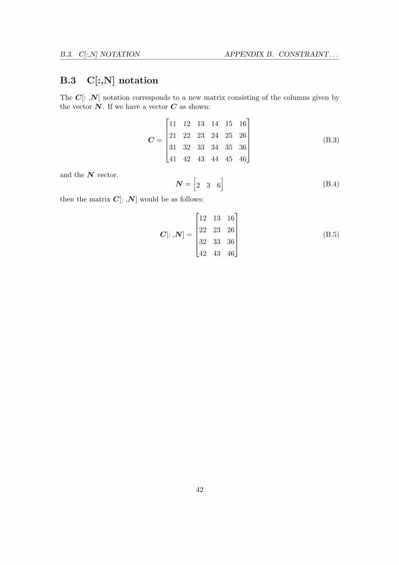
B.3 C[:,N] notation

The C[: ,N ] notation corresponds to a new matrix consisting of the columns given bythe vector N . If we have a vector C as shown:

C =

11 12 13 14 15 16

21 22 23 24 25 26

31 32 33 34 35 36

41 42 43 44 45 46

(B.3)

and the N vector.N =

[2 3 6

](B.4)

then the matrix C[: ,N ] would be as follows:

C[: ,N ] =

12 13 16

22 23 26

32 33 36

42 43 46

(B.5)

42

CPower and Friction Calculations

43

C.1. POWER SPLIT APPENDIX C. POWER AND . . .

C.1 Power split

The power is divided between the X/Y and F/R clutch pairs in the following way. Firstthe theoretical power lost can be described by using the equations below:

Pt,Cx/Cy= µx ∗ Fx ∗Nx ∗ |∆ωx| ∗

Ro,x∫Ri,x

dr + µy ∗ Fy ∗Ny ∗ |∆ωy| ∗Ro,y∫Ri,y

dr

Pt,Cf/Cr= µf ∗ Ff ∗Nf ∗ |∆ωf | ∗

Ro,f∫Ri,f

dr + µr ∗ Fr ∗Nr ∗ |∆ωr| ∗Ro,r∫Ri,r

dr

(C.1)

An explanation of all the parameters can be seen in the following table:

Table C.1: Parameters for calculating the theoretical power loss in clutches.

Pt Theoretical. power loss

µ COF

F Clamp force

N Number of friction interfaces

|∆ω| Slip speed

Ro Outer radius of friction disc

Ri Inner radius of friction disc

The sum of the power loss in each pair is equal to the total power loss in all clutchesas given in:

Pall cl. = PCx/Cy+ PCf/Cr

(C.2)

The ratio between the two theoretical power losses can be calculated by the followingequation:

Pt,Cx/Cy

Pt,Cf/Cr

=

µx ∗ Fx ∗Nx ∗ |∆ωx| ∗Ro,x∫Ri,x

dr + µy ∗ Fy ∗Ny ∗ |∆ωy| ∗Ro,y∫Ri,y

dr

µf ∗ Ff ∗Nf ∗ |∆ωf | ∗Ro,f∫Ri,f

dr + µr ∗ Fr ∗Nr ∗ |∆ωr| ∗Ro,r∫Ri,r

dr

= kxy/fr

(C.3)This can then be rewritten in the following form:

PCx/Cy= kxy/fr ∗ PCf/Cr

(C.4)

44

C.1. POWER SPLIT APPENDIX C. POWER AND . . .

Combined with equation C.2 to get the power loss in each clutch pair.

Pall cl. = kxy/fr ∗ PCf/Cr+ PCf/Cr

Pall cl. = PCf/Cr(kxy/fr + 1)

PCf/Cr=

Pall cl.

(kxy/fr + 1)

PCx/Cy=

Pall cl.(1 +

1

kxy/fr

)(C.5)

The power is split using the same method for the clutches in each pair. The theoreticalpower loss in each speed clutch can be calculated with the following equations:

Pt,x = µx ∗ Fx ∗Nx ∗ |∆ωx| ∗Ro,x∫Ri,x

dr

Pt,y = µy ∗ Fy ∗Ny ∗ |∆ωy| ∗Ro,y∫Ri,y

dr

(C.6)

The total power loss in the clutch pair can be described with the following equation:

PCx/Cy= Px + Py (C.7)

The ratio is then calculated with the following equation:

Pt,x

Pt,y=

µx ∗ Fx ∗Nx ∗ |∆ωx| ∗Ro,x∫Ri,x

dr

µy ∗ Fy ∗Ny ∗ |∆ωy| ∗Ro,y∫Ri,y

dr

= kx/y (C.8)

and can be rewritten in the following form:

Px = kx/y ∗ Py (C.9)

By combining this with equation C.7 one can calculate the power loss in each clutch:

PCx/Cy= kx/y ∗ Py + Py

PCx/Cy= Py(kx/y + 1)

Py =PCx/Cy

(kx/y + 1)

Px =PCx/Cy(

1 +1

kx/y

)(C.10)

45

C.2. COF APPENDIX C. POWER AND . . .

The theoretical power loss in each direction clutch can be calculated with the followingequations:

Pt,f = µf ∗ Ff ∗Nf ∗ |∆ωf | ∗Ro,f∫Ri,f

dr

Pt,y = µr ∗ Fr ∗Nr ∗ |∆ωr| ∗Ro,r∫Ri,r

dr

(C.11)

Total power loss in the clutch pair can be described with the following equation:

PCf/Cr= Pf + Pr (C.12)

The ratio is then calculated with the following equation:

Pt,f

Pt,r=

µf ∗ Ff ∗Nf ∗ |∆ωf | ∗Ro,f∫Ri,f

dr

µr ∗ Fr ∗Nr ∗ |∆ωr| ∗Ro,r∫Ri,r

dr

= kf/r (C.13)

which can be rewritten in the following form:

Pf = kf/r ∗ Pr (C.14)

By combining this with equation C.12 one can calculate the power loss in each clutch:

PCf/Cr= kf/r ∗ Pr + Pr

PCf/Cr= Pr(kf/r + 1)

Pr =PCf/Cr

(kf/r + 1)

Pf =PCf/Cr(

1 +1

kf/r

)(C.15)

C.2 COF

The COF can be calculated by comparing the theoretical power loss (Pt,n) and the actualpower loss(Pmodel) to see what the COF should be so that they are equal.

Pmodel = Pt,n

Pmodel = µ ∗ F ∗N ∗ |∆ω| ∗Ro∫

Ri

dr

µ =Pmodel

F ∗N ∗ |∆ω| ∗Ro∫Ri

dr

(C.16)

46

DCalculation Scripts

47

D.1. MAIN CALCULATION SCRIPT APPENDIX D. CALCULATION . . .

D.1 Main calculation script

Figure D.1: Flowchart of the main calculations script.

48

D.2. INTERMEDIATE SPEED . . . APPENDIX D. CALCULATION . . .

D.2 Intermediate speed calculations.

Figure D.2: Flowchart of the script that calculates the intermediate speed.

D.3 Rotation direction fix

The rotation direction is corrected by identifying the point where a change would occurand then changing the direction between each point pair. A point where a change willoccur is identified by the following conditions:

ωx ≤ ωthres.

ωoutp. < 0

dωx

dt= 0

(D.1)

where ωx is the rotation speed that is being precessed, ωthres. is a threshold value thatdescribes the highest speed where an inversion can occur and ωoutp. is the output speedfrom the transmission.

49

D.4. COF CALCULATIONS APPENDIX D. CALCULATION . . .

The points are then divided into pairs. If there is an uneven amount of point thenan error message will be logged. The rotation speed is then inverted between the pointsin each pair. It is assumed that rotation will occur in a positive direction at the start ofthe sequence.

D.4 COF calculations

Figure D.3: Flowchart of the script that calculates the COF of the clutches.

50