Atmos. Chem. Phys., 17, 12633–12643, 2017https://doi.org/10.5194/acp-17-12633-2017© Author(s) 2017. This work is distributed underthe Creative Commons Attribution 3.0 License.

What controls the seasonal cycle of columnar methane observed byGOSAT over different regions in India?Naveen Chandra1,a, Sachiko Hayashida1, Tazu Saeki2,b, and Prabir K. Patra2

1Faculty of Science, Nara Women’s University, Kita-Uoya Nishimachi, Nara 630-8506, Japan2Department of Environmental Geochemical Cycle Research, JAMSTEC, Yokohama 2360001, Japananow at: Research and Development Center for Global Change, JAMSTEC, Yokohama 2360001, Japanbnow at: Center for Global Environmental Research, National Institute for Environmental Studies, Tsukuba 305-8506, Japan

Correspondence to: Naveen Chandra (nav.phy09@gmail.com)

Received: Received on 13 – Discussion started: 26 April 2017Revised: 14 August 2017 – Accepted: 11 September 2017 – Published: 24 October 2017

Abstract. Methane (CH4) is one of the most important short-lived climate forcers for its critical roles in greenhouse warm-ing and air pollution chemistry in the troposphere, and thewater vapor budget in the stratosphere. It is estimated thatup to about 8 % of global CH4 emissions occur from SouthAsia, covering less than 1 % of the global land. With theavailability of satellite observations from space, variabil-ity in CH4 has been captured for most parts of the globalland with major emissions, which were otherwise not cov-ered by the surface observation network. The satellite ob-servation of the columnar dry-air mole fractions of methane(XCH4) is an integrated measure of CH4 densities at all alti-tudes from the surface to the top of the atmosphere. Here,we present an analysis of XCH4 variability over differentparts of India and the surrounding cleaner oceanic regionsas measured by the Greenhouse gases Observation SATel-lite (GOSAT) and simulated by an atmospheric chemistry-transport model (ACTM). Distinct seasonal variations ofXCH4 have been observed over the northern (north of 15◦ N)and southern (south of 15◦ N) parts of India, corresponding tothe peak during the southwestern monsoon (July–September)and early autumn (October–December) seasons, respectively.Analysis of the transport, emission, and chemistry contribu-tions to XCH4 using ACTM suggests that a distinct XCH4seasonal cycle over northern and southern regions of Indiais governed by both the heterogeneous distributions of sur-face emissions and a contribution of the partial CH4 columnin the upper troposphere. Over most of the northern IndianGangetic Plain regions, up to 40 % of the peak-to-troughamplitude during the southwestern (SW) monsoon season

is attributed to the lower troposphere (∼ 1000–600 hPa),and ∼ 40 % to uplifted high-CH4 air masses in the uppertroposphere (∼ 600–200 hPa). In contrast, the XCH4 sea-sonal enhancement over semi-arid western India is attributedmainly (∼ 70 %) to the upper troposphere. The lower tro-pospheric region contributes up to 60 % in the XCH4 sea-sonal enhancement over the Southern Peninsula and oceanicregion. These differences arise due to the complex atmo-spheric transport mechanisms caused by the seasonally vary-ing monsoon. The CH4 enriched air mass is uplifted from ahigh-emission region of the Gangetic Plain by the SW mon-soon circulation and deep cumulus convection and then con-fined by anticyclonic wind in the upper tropospheric heights(∼ 200 hPa). The anticyclonic confinement of surface emis-sion over a wider South Asia region leads to a strong con-tribution of the upper troposphere in the formation of theXCH4 peak over northern India, including the semi-arid re-gions with extremely low CH4 emissions. Based on this anal-ysis, we suggest that a link between surface emissions andhigher levels of XCH4 is not always valid over Asian mon-soon regions, although there is often a fair correlation be-tween surface emissions and XCH4. The overall validity ofACTM simulation for capturing GOSAT observed seasonaland spatialXCH4 variability will allow us to perform inversemodeling ofXCH4 emissions in the future usingXCH4 data.

Published by Copernicus Publications on behalf of the European Geosciences Union.

12634 N. Chandra et al.: Controlling factors for XCH4 seasonality over India

1 Introduction

Methane (CH4) is the second most important anthropogenicgreenhouse gas (GHG) after carbon dioxide (CO2) and ac-counts for ∼ 20 % (+0.97 Wm−2) of the increase in total di-rect radiative forcing since 1750 (Myhre et al., 2013). CH4is emitted from a range of anthropogenic and natural sourceson the Earth’s surface into the atmosphere. The main natu-ral sources of CH4 include wetlands and termites (Matthewsand Fung, 1987; Cao et al., 1998; Sugimoto et al., 1998).Livestock, rice cultivation, the fossil fuel industry (produc-tion and uses of natural gas, oil, and coal), and landfills arethe major sectors among the anthropogenic sources (Crutzenet al., 1986; Minami and Neue, 1994; Olivier et al., 2005; Yanet al., 2009). These results also suggest that the Asian regionis an emission hotspot of CH4 due to the large number of live-stock, intense cultivation, coal mining, waste management,and other anthropogenic activities (EDGAR2FT, 2013).

With a short atmospheric lifetime of about 10 years (e.g.,Patra et al., 2011a) and having 34 times more potential totrap heat than CO2 on a mass basis over a 100-year timescale(Gillett and Matthews, 2010; Myhre et al., 2013), mitiga-tion of CH4 emissions could be the most important way tolimit global warming at inter-decadal timescales (Shindellet al., 2009). Better knowledge of CH4 distribution and quan-tification of its emission flux is indispensable for assessingpossible mitigation strategies. However, sources of CH4 arenot yet well quantified due to sparse ground-based measure-ments, which results in limited representation of CH4 fluxon a larger scale (Dlugokencky et al., 2011; Patra et al.,2016). Recent technological advances have made it possi-ble to detect spatial and temporal variations in atmosphericCH4 from space (Frankenberg et al., 2008; Kuze et al., 2009),which could fill the gaps left by ground-, aircraft- and ship-based measurements, albeit at a lower accuracy than thein situ measurements. Further, despite the satellite obser-vations having an advantage of providing continuous mon-itoring over a wide spatial range, the information obtainedfrom passive nadir sensors that use solar radiation at theshort-wavelength infrared (SWIR) spectral band is limited tocolumnar dry-air mole fractions of methane (XCH4). Thisis an integrated measure of CH4 with contributions from thedifferent vertical atmospheric layers, i.e., from the measure-ment point on the Earth’s surface to the top of the atmosphere(up to about 100 km or more precisely to the satellite orbit).

The South Asia region, consisting of India, Pakistan,Bangladesh, Nepal, Bhutan, and Sri Lanka, exerts a signif-icant impact on the global CH4 emissions, with regionaltotal emissions of 37± 3.7 Tg CH4 of about 500 Tg CH4global total emissions during the 2000s (Patra et al., 2013).The Indo-Gangetic Plain (IGP) located in the foothills ofthe Himalayas is one of the most polluted regions in theworld, hosts 70 % of coal-fired thermal power plants in In-dia, and experiences intense agricultural activity (Kar et al.,2010). This region is of particular interest mainly due to the

coexistence of deep convection and large emission of pol-lutants (including CH4) from a variety of natural and an-thropogenic sources. Rainfall during the SW monsoon sea-son causes higher CH4 emissions from the paddy fields andwetlands (e.g., Matthews and Fung, 1987; Yan et al., 2009;Hayashida et al., 2013), while the persistent deep convectionresults in updraft of CH4-laden air mass from the surface tothe upper troposphere during the same season, which is thenconfined by anticyclonic winds at this height (Patra et al.,2011b; Baker et al., 2012; Schuck et al., 2012). Several otherstudies have also highlighted the role of convective transportof pollutants (including CH4) from the surface to the up-per troposphere (400–200 hPa) during the SW monsoon sea-son (July–September) (Park et al., 2004; Randel et al., 2006;Xiong et al., 2009; Lal et al., 2014; Chandra et al., 2016).The dynamical system dominated by deep convection andanticyclone covers mostly the northern Indian region (northof 15◦ N) due to the presence of the Himalayas and the Ti-betan Plateau, while such a complex dynamical system hasnot been observed over the southern part of India (south of15◦ N) (Rao, 1976).

Satellite-based measurements show elevated levels ofXCH4 over the northern part of India (north of 15◦ N) tobe particularly high over the IGP during the SW monsoonseason (July–September) and over southern India (south of15◦ N) during the early autumn season (October–December)(Frankenberg et al., 2008, 2011; Hayashida et al., 2013).Previous studies have linked these high XCH4 levels to thestrong surface CH4 emissions particularly from the rice cul-tivation over the Indian region because they showed statisti-cally significant correlations over certain regions (Hayashidaet al., 2013; Kavitha et al., 2016). The differences in the peakof the XCH4 seasonal cycle over the northern and southernregions of India are also discussed on the basis of agricul-tural practice in India that takes place in two seasons, May–October and November–April, respectively. However, infer-ring local emissions directly from variations in XCH4 is am-biguous, particularly over the Indian regions under the influ-ence of monsoon meteorology, because XCH4 involves con-tributions of CH4 abundances from all altitudes along the so-lar light path.

This study attempts for the first time to separate the factorsresponsible (emission, transport, and chemistry) for the dis-tributions of columnar methane (XCH4) over the Asian mon-soon region for different altitude segments. The XCH4 mix-ing ratios are used for this study as observed from GOSATand simulated by JAMSTEC’s ACTM. We aim to understandrelative contributions of surface emissions and transport inthe formation of XCH4 seasonal cycles over different partsof India and the surrounding oceans. This understanding willhelp us in developing an inverse modeling system for estima-tion of CH4 surface emissions using XCH4 observations andACTM forward simulation.

Atmos. Chem. Phys., 17, 12633–12643, 2017 www.atmos-chem-phys.net/17/12633/2017/

N. Chandra et al.: Controlling factors for XCH4 seasonality over India 12635

2 Methods

2.1 Satellite data

The Greenhouse gases Observing SATellite (GOSAT) (alsoreferred to as Ibuki) project is developed jointly by the Na-tional Institute for Environmental Studies (NIES), Ministryof the Environment (MOE), and Japan Aerospace Explo-ration Agency (JAXA). It has been providing columnar dry-air mole fractions of the two important greenhouse gases(XCH4 and XCO2) at near-global coverage since its launchin January 2009. It is equipped onboard with the ThermalAnd Near infrared Sensor for carbon Observation-FourierTransform Spectrometer (TANSO-FTS) and the Cloud andAerosol Imager (TANSO-CAI) (Kuze et al., 2009). To avoidcloud contamination in the retrieval process, any scene withmore than 1 cloudy pixel within the TANSO-FTS IFOV is ex-cluded. The atmospheric images from CAI are used to iden-tify the cloudy pixels. As a result of this strict screening, onlylimited numbers of XCH4 data are available during the SWmonsoon over South Asia. This study uses the GOSAT SWIRXCH4 (Version 2.21)-Research Announcement product forthe period of 2011–2014. The ground-based FTS measure-ments ofXCH4 by the Total Carbon Column Observing Net-work (TCCON) (Wunch et al., 2011) are used extensivelyto validate the GOSAT retrievals. Retrieval bias and preci-sion of column abundance from GOSAT SWIR observationshave been estimated as approximately 15–20 ppb and 1 %, re-spectively, for the NIES product using TCCON data (Morinoet al., 2011; Yoshida et al., 2013).

2.2 Model simulations

Model analysis is comprised of simulations from JAM-STEC’s atmospheric general circulation model (AGCM)-based chemistry-transport model (ACTM; Patra et al.,2009). The AGCM was developed by the Center for Cli-mate System Research/National Institute for Environmen-tal Studies/Frontier Research Center for Global Change(CCSR/NIES/FRCGC). It has been part of transport modelintercomparison experiment TransCom-CH4 (Patra et al.,2011a) and used in inverse modeling of CH4 emissionsfrom in situ observations (Patra et al., 2016). The ACTMruns at a horizontal resolution of T42 spectral truncations(∼ 2.8◦× 2.8◦) with 67 sigma-pressure vertical levels. Theevolution of CH4 at different longitude (x), latitude (y), andaltitude (z) with time in the Earth’s atmosphere depends onthe surface emission, chemical loss, and transport, which canbe mathematically represented by the following continuityequation:

dCH4 (x,y,z, t)

dt= SCH4 (x,y, t)− LCH4 (x,y,z, t)

−∇φ (x,y,z, t) ,

where CH4 is the methane burden in the atmosphere, SCH4 isthe total emissions/sinks of CH4 at the surface, LCH4 is thetotal loss of CH4 in the atmosphere due to the chemical re-actions, and ∇φ is the transport of CH4 due to the advection,convection, and diffusion.

The meteorological fields of ACTM are nudged with re-analysis data from the Japan Meteorological Agency, ver-sion JRA-25 (Onogi et al., 2007). The model uses an opti-mal OH field (Patra et al., 2014) based on a scaled version ofthe seasonally varying OH field (Spivakovsky et al., 2000).The a priori anthropogenic emissions are from the EmissionDatabase for Global Atmospheric Research (EDGAR) v4.2FT2010 (http://edgar.jrc.ec.europa.eu). The model sensitivityfor emission is examined by two cases of emission scenariosbased on different combinations of sectoral emissions. Thefirst one is referred to as the “AGS”, where all emission sec-tors in EDGAR42FT are kept at a constant value for 2000,except for emissions from agriculture soils. The second oneis a controlled emission scenario referred to as “CTL”, whichis based on the ensemble of the anthropogenic emissionsfrom EDGAR32FT (as in Patra et al., 2011a), wetland andbiomass burning emissions from Fung et al. (1991), and ricepaddy emission from Yan et al. (2009). The emission season-ality differs substantially between the CTL case and the AGScase due to differences in emissions from wetlands, rice pad-dies, and biomass burning; other anthropogenic emissions donot contain seasonal variations (Patra et al., 2016). Furtherdetails about the model and these emission scenarios canbe found in the previous studies (Patra et al., 2009, 2011a,2016).XCH4 is calculated from the ACTM profile using the fol-

lowing equations:

XCH4 =

60∑n=1

CH4(n)×1σp(n),

where CH4(n) is the dry-air mole fraction at model mid-point level, n= number of vertical sigma pressure layersof ACTM (= 1–60 with σp values of 1.0 and 0.005), and1σp = thickness of the sigma pressure level. Note here thatwe have not incorporated convolution of model profiles withretrieval a priori and averaging kernels. Because the averag-ing kernels are nearly constant in the troposphere (Yoshidaet al., 2011), this approximation does not lead to serious er-rors in constructing the model XCH4. For both the CTL andAGS cases, we adjust a constant offset of 20 ppb to the mod-eled time series, which should make the a priori correctionhave a lesser impact on the model XCH4. Because the fo-cus of this study is seasonal and spatial variations in XCH4,a constant offset adjustment should not affect the main con-clusions.

www.atmos-chem-phys.net/17/12633/2017/ Atmos. Chem. Phys., 17, 12633–12643, 2017

12636 N. Chandra et al.: Controlling factors for XCH4 seasonality over India

(a1) GOSAT XCH (AMJ)4

60° E 70° E 80° E 90° E 100° E0°

10° N

20° N

30° N

(a2) GOSAT XCH (OND)4

1750 1770 1790 1810 1830 1850 1870XCH4 (ppb)

(b1) ACTM XCH (AMJ)4

(b2) ACTM XCH (OND)4

1750 1770 1790 1810 1830 1850 1870XCH4 (ppb)

(c1) Surface flux (AMJ)

(c2) Surface flux (OND)

0.1 2.0 10.0 50.0120.0gCH4 m-2 month-1 : AGS

60° E 70° E 80° E 90° E 100° E 60° E 70° E 80° E 90° E 100° E 60° E 70° E 80° E 90° E 100° E

60° E 70° E 80° E 90° E 100° E 60° E 70° E 80° E 90° E 100° E

0°

10° N

20° N

30° N

0°

10° N

20° N

30° N

0°

10° N

20° N

30° N

0°

10° N

20° N

30° N

0°

10° N

20° N

30° N

Figure 1. Average seasonal distributions (from 2011 to 2014) of XCH4 obtained from GOSAT observations (a1, a2), ACTM simulations(b1, b2), and CH4 emission consisting of all the natural and anthropogenic emissions (c1, c2: ACTM_AGS case) over the Indian region.Optimized emissions are shown from a global inversion of surface CH4 concentrations (Patra et al., 2016) and multiplied by a constant factorof 12 for a clear visualization. The ACTM is first sampled at the location and time of GOSAT observations and then seasonally averaged.The white spaces in first two columns (a1, a2, b1, b2) are due to the missing data caused by satellite retrieval limitations under cloud cover.

3 Results and discussion

3.1 XCH4 over the Indian region: view from GOSATand ACTM simulations

This section presents an analysis of XCH4 observed byGOSAT from January 2011 to December 2014 over the In-dian region. We characterize the four seasons specific tothe region as winter (January–March), spring (April–June),summer (July–September) or the SW monsoon, and autumn(October–December), as commonly used in meteorologicalstudies (e.g., Rao, 1976). To study the seasonalXCH4 patternin detail depending on the distinct spatial pattern of surfaceemissions and XCH4 mixing ratios shown in Fig. 1, the In-dian landmass was partitioned into eight sub-regions: North-east India (NEI), Eastern India (EI), Eastern IGP (EIGP),Western IGP (WIGP), Central India (CI), Arid India (AI),Western India (WI), Southern Peninsula (SP), and two sur-rounding oceanic regions, the Arabian Sea (AS) and the Bayof Bengal (BOB) (Fig. 2a). Regional divisions are madebased on spatial patterns of emission and XCH4 (Fig. 1a1–c2) and our knowledge of seasonal meteorological condi-tions. Since general features of XCH4 simulated by ACTMusing emission scenarios AGS and CTL are similar to eachother, the main discussion is carried out using the AGS sce-nario only.

Figure 1a1–a2 show that theXCH4 mixing ratios are lowerin spring and higher in autumn. A strong latitudinal gradientin XCH4 is observed between the Indo-Gangetic Plain (IGP)

and the other parts of India. XCH4 shows the highest value(∼ 1880 ppb) over the IGP, eastern, and northeastern Indianregions. As seen from Fig. 1b1–b2, ACTM simulations areable to reproduce the observed latitudinal and seasonal gra-dients in XCH4, i.e., higher values during the southwesternmonsoon and autumn seasons and lower values during thewinter and spring seasons over the IGP region. The opti-mized total CH4 fluxes (AGS and CTL) show high emissionsover the IGP and northeastern Indian regions (Fig. 1c1–c2).Most elevated levels of XCH4 are often observed simultane-ously with the higher emissions, suggesting a link betweenthe enhanced XCH4 and high surface emissions in summer.However, this link is not valid for all locations. For exam-ple, over the western and southern regions of India, XCH4is higher in autumn than in spring, though the emissions arehigher in spring.

Figure 2b–k show ACTM–GOSAT comparisons of XCH4time series from January 2011 to December 2014 over the se-lected study regions. The simulated XCH4 data are sampledat the nearest model grid to the available GOSAT observa-tions and at the satellite overpass time (∼ 13:00 LT) and thenaveraged over each study region. Observations are sparse ornot available during the SW monsoon season in some of theregions due to limitations of GOSAT retrieval under cloudcover. The model captures the salient features of the seasonalcycles at very high statistical significance (correlation coef-ficients, r > 0.8; except for northeastern India; Table 1). Thehigh ACTM-GOSAT correlations for the low-/no-emissionregions suggest that transport and chemistry are accurately

Atmos. Chem. Phys., 17, 12633–12643, 2017 www.atmos-chem-phys.net/17/12633/2017/

N. Chandra et al.: Controlling factors for XCH4 seasonality over India 12637

Figure 2. (a) The map of the regional divisions (shaded) for the time series analysis. (b–k) Time series of XCH4 over the selected regions(shown on the map) as obtained from GOSAT and simulated by ACTM for two different emission scenarios, namely, ACTM_AGS andACTM_CTL. The gaps are due to the missing observational data.

modeled in ACTM. Although we do not have the statisti-cally significant number of observations for the SW monsoonperiod, the observed high GOSAT XCH4 are generally wellsimulated by ACTM over most of the study regions. Basedon these comparisons, we can assume that model simula-tions can be used to understand XCH4 variability over theIndian region. Though we showed only the paired GOSATand ACTM data that matched in time and location in Fig. 2b–k, we also confirmed that the correlation is high (r ∼ 0.9)between the monthly averaged time series of GOSAT andACTM averaged for the 4 years (2011–2014) when ACTMis not co-sampled at the GOSAT sampling points (Fig. S1 inthe Supplement). These high correlations ensure representa-tiveness of the data shown in Fig. 2b–k. Thus, the seasonalevolution of XCH4 using the ACTM simulations alone is ex-pected to be fairly valid for different altitude layers (referto Patra et al., 2011b, for comparison at the aircraft cruisingaltitude). Though the model is only validated for XCH4 inthis study, comparisons with surface and independent aircraftCH4 observations have been shown in Patra et al. (2016).

3.2 Seasonal cycle of XCH4 and possible controllingfactors

As mentioned earlier, the persistent deep convection andmean circulation during the SW monsoon season signifi-cantly enhance CH4 in the upper troposphere (e.g., Xionget al., 2009; Baker et al., 2012), coinciding with the period

Table 1. Correlation coefficients (r) between observed and modelsimulated seasonal cycles of XCH4. Model simulations are ob-tained from ACTM using two different emission scenarios, AGSand CTL.

Site/tracer ACTM_AGS ACTM_CTL

Arid India 0.77 0.88WIGP region 0.86 0.90EIGP region 0.69 0.88Northeast India 0.55 0.55Western India 0.87 0.95Central India 0.89 0.97East India 0.78 0.86Southern Peninsula 0.92 0.91Arabian Sea 0.86 0.87Bay of Bengal 0.84 0.86

of high surface CH4 emissions due to rice paddy cultiva-tion and wetlands over the Indian region (Yan et al., 2009;Hayashida et al., 2013). Although both these emissions andtransport processes contribute greatly to seasonal changes inXCH4, their relative contributions have not been studied overthe monsoon-dominated Indian region.

To understand the role of transport, the atmospheric col-umn is segregated into five sigma-pressure (σp) layers, start-ing from the surface level (σp = 1) to the top of the atmo-sphere (σp = 0), with an equal layer thickness of σp = 0.2.

www.atmos-chem-phys.net/17/12633/2017/ Atmos. Chem. Phys., 17, 12633–12643, 2017

12638 N. Chandra et al.: Controlling factors for XCH4 seasonality over India

Figure 3. The bottom panels show the monthly mean climatology of the total optimized CH4 emissions (a7, b7, c7), estimated after perform-ing the global inverse analysis (Patra et al., 2016). The second bottom panels show XCH4 obtained from the GOSAT observations (blackcircles in a6, b6, c6) and ACTM simulations (a6, b6, c6) over the Eastern IGP (column a), Southern Peninsula (column b) and Arid India(column c) regions. Monthly climatology is based on the monthly mean values for the period of 2011–2014 for all the values. The error barsin the GOSAT monthly mean values depict the 1-σ SDs for the corresponding months (a6, b6, c6). The 1-σ values are not plotted for themodel simulations to maintain figure clarity. Simulations are based on two different emission scenarios, namely, ACTM_CTL (blue lines)and ACTM_AGS (red lines) based on the different combinations of emissions. The upper five panels show the monthly climatology of partialcolumnar methane (denoted by XpCH4) calculated at five different partial sigma-pressure layers: 1.0–0.8 (a5, b5, c5), 0.8–0.6 (a4, b4, c4),0.6–0.4 (a3, b3, c3), 0.4–0.2 (a2, b2, c2), and 0.2–0.0 (a1, b1, c1). Please note that the y scales in the emission plots over the SouthernPeninsula and Arid India (b7, c7) are different from over the EIGP region (a7).

Lower Troposphere (LT), Mid-Troposphere1 (MT1), Mid-Troposphere2 (MT2), Upper Troposphere (UT), and UpperAtmosphere (UA) denote the layers corresponding to thesigma-pressure values of 1.0–0.8, 0.8–0.6, 0.6–0.4, 0.4–0.2,and 0.2–0.0. The partial columnar CH4 is calculated withindifferent σp layers (denoted by XpCH4) using the same for-mula for XCH4, as in Sect. 2.2. The model results are aver-aged over each sub-region of our analysis for the XCH4 sea-sonal cycle. To understand the role of surface emission in theXCH4 seasonal cycle, the climatology of the optimized totalCH4 flux for each sub-region is compared. Figure 3 showsthe monthly mean climatology (average for 2011–2014) oftotal CH4 flux, XCH4, and XpCH4 from the model aver-aged over three selected regions, EIGP (a1–a7), SP (b1–b7),and AI (c1–c7). These representative regions have been se-lected because they show distinct XCH4 seasonal cycles andthe dominant controlling factors (such as emission, transport,and chemistry). The observed GOSAT XCH4 values are alsoshown for a reference; however, the model results do not cor-respond to the location and time of GOSAT observations (as

opposed to those in Fig. 2). The plots for the remaining sevenregions are available in Figs. S2 and S3.

Over the EIGP region, the magnitude and timing of theseasonal peak in emission differ substantially between theCTL and AGS emission scenarios (refer to Fig. 3a7). ACTMsimulatedXCH4 seasonal peak is in agreement with the peakin emission in June for the AGS case (Fig. 3a6). However,simulated XCH4 remains nearly constant until September,although the emission decreases substantially toward win-ter. In general, the emission is relatively higher in the mon-soon season (July–August–September) than in other sea-sons in both cases. However, in the LT, where we expectmost susceptibility to the surface emission, the partial col-umn CH4 indicates very different seasonality from the emis-sions; XpCH4 (LT) increases toward winter continuously(Fig. 3a5). The partial CH4 columns for the upper tropo-sphere and middle troposphere (Fig. 3a2–a3) show similarseasonality to the total XCH4 rather than in the LT. There-fore, this analysis strongly suggests that the emissions fromthe surface and the upper tropospheric partial column both

Atmos. Chem. Phys., 17, 12633–12643, 2017 www.atmos-chem-phys.net/17/12633/2017/

N. Chandra et al.: Controlling factors for XCH4 seasonality over India 12639

contribute to the formation of the XCH4 seasonal cycle.These results also suggest the possibility that GOSAT andACTM XCH4 data can be used for correcting a priori emis-sion scenarios by inverse modeling.

In contrast to the XCH4 seasonal cycle over EIGP, a no-table difference is observed in the emission and XCH4 sea-sonal cycle over the SP region (Fig. 3b). The XCH4 sea-sonal cycle and emission seasonal cycle are found to beout of phase with each other and the differences in emis-sion scenarios are not reflected in XCH4 seasonal variations.Both emission scenarios show the distinct seasonal pattern:AGS shows annual high emissions from April to September,while CTL shows an annual high during August–September(Fig. 3b7). The total emissions over SP are much lower thanthat of EIGP (note the different y axis scale for Fig. 3b7) andhence the difference between the XCH4 simulations fromboth emission scenarios is comparatively low. The XCH4shows almost identical seasonal cycles for both of the emis-sion scenarios, a peak in October, and prolonged low val-ues during May–September. The seasonal XpCH4 cycle inthe LT layer shows the seasonal pattern similar to the to-tal XCH4. Inconsistency between emission seasonality andXCH4 coupled with low emissions strongly suggests that theXCH4 can be controlled by transport and/or chemistry butnot emissions. Surface winds during May–September overSP are of marine origin, which effectively flushes the airwith low CH4 (see Fig. S4). Further, the distinct seasonalcycle of chemical loss is observed over the SP region com-pared to other study regions; the loss rate starts increasingfrom 6 ppbday−1 in January to 12 ppbday−1 in April, andcontinues to remain high until September (refer to Fig. S5).These pieces of evidence clearly suggest that the combinedeffect of transport and chemistry causes the low XCH4 val-ues for the May–September period over the SP region. Thepeaks in the upper layers in October (Fig. 3b1–b4) and trans-port from the polluted continental layer in the LT layer (referto Fig. S4) could together contribute to the seasonal XCH4peak over SP. Based on these findings, we conclude that theXCH4 measurements do not impose a strong constraint onsurface emissions for inverse modeling over the SP region,suggesting a need for in situ measurements.

Over the Arid India (AI) region, the XCH4 seasonal cy-cle is observed to be different from those of the EIGP andSI regions. The simulated XCH4 (Fig. 3c6) shows extremelyweak sensitivity to the surface emission differences betweenthe AGS and CTL cases (Fig. 3c7). Additionally, theXpCH4in the LT layer (Fig. 3c5) does not resemble the phase of sea-sonality in surface emissions and simulated/observedXCH4.The XpCH4 in the LT layer decreases from January to Au-gust and increases until December. On the other hand, a re-markable peak (∼ 1896 ppb) is observed in XCH4 duringAugust, followed by a decline afterward (Fig. 3c6). This isan outstanding example of deceiving linkage between surfaceemissions and XCH4 in terms of seasonal variation. An en-hancement in the mixing ratios of XpCH4 is observed from

-20

0

20

40

60

80

100

AI WIGP EIGP NEI EI CI WI SP AS BOBCon

trib

utio

n fr

om d

iffer

ent l

ayer

s (%

)

Region

UAUTMT2MT1LT

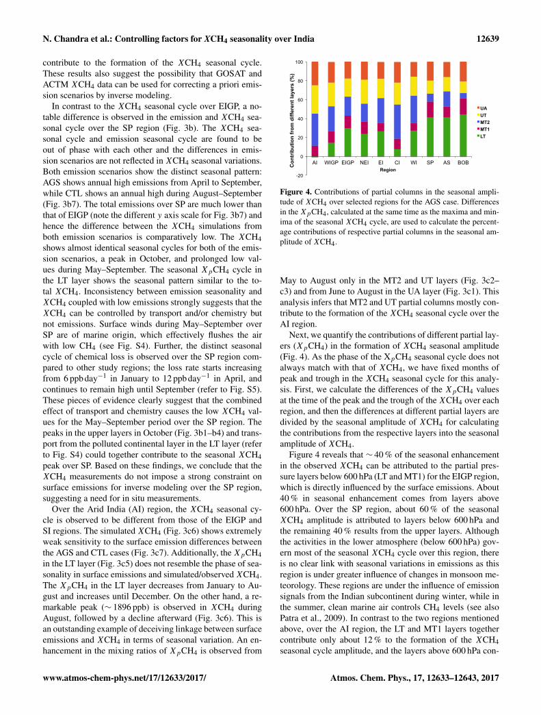
Figure 4. Contributions of partial columns in the seasonal ampli-tude of XCH4 over selected regions for the AGS case. Differencesin the XpCH4, calculated at the same time as the maxima and min-ima of the seasonal XCH4 cycle, are used to calculate the percent-age contributions of respective partial columns in the seasonal am-plitude of XCH4.

May to August only in the MT2 and UT layers (Fig. 3c2–c3) and from June to August in the UA layer (Fig. 3c1). Thisanalysis infers that MT2 and UT partial columns mostly con-tribute to the formation of the XCH4 seasonal cycle over theAI region.

Next, we quantify the contributions of different partial lay-ers (XpCH4) in the formation of XCH4 seasonal amplitude(Fig. 4). As the phase of the XpCH4 seasonal cycle does notalways match with that of XCH4, we have fixed months ofpeak and trough in the XCH4 seasonal cycle for this analy-sis. First, we calculate the differences of the XpCH4 valuesat the time of the peak and the trough of the XCH4 over eachregion, and then the differences at different partial layers aredivided by the seasonal amplitude of XCH4 for calculatingthe contributions from the respective layers into the seasonalamplitude of XCH4.

Figure 4 reveals that ∼ 40 % of the seasonal enhancementin the observed XCH4 can be attributed to the partial pres-sure layers below 600 hPa (LT and MT1) for the EIGP region,which is directly influenced by the surface emissions. About40 % in seasonal enhancement comes from layers above600 hPa. Over the SP region, about 60 % of the seasonalXCH4 amplitude is attributed to layers below 600 hPa andthe remaining 40 % results from the upper layers. Althoughthe activities in the lower atmosphere (below 600 hPa) gov-ern most of the seasonal XCH4 cycle over this region, thereis no clear link with seasonal variations in emissions as thisregion is under greater influence of changes in monsoon me-teorology. These regions are under the influence of emissionsignals from the Indian subcontinent during winter, while inthe summer, clean marine air controls CH4 levels (see alsoPatra et al., 2009). In contrast to the two regions mentionedabove, over the AI region, the LT and MT1 layers togethercontribute only about 12 % to the formation of the XCH4seasonal cycle amplitude, and the layers above 600 hPa con-

www.atmos-chem-phys.net/17/12633/2017/ Atmos. Chem. Phys., 17, 12633–12643, 2017

12640 N. Chandra et al.: Controlling factors for XCH4 seasonality over India

0.0

0.0

0.015.0

30.0

0° 10° N 20° N 30° N 40° N1000

500

300

200

100

50

-15.0

0.0

0.0

1000

500

300

200

100

50

-30.0-15.0

-15.0

0.0

1000

500

300

200

100

50

-30.0

-15.0

0.0

0.0

1000

500

300

200

100

50

-10 -8 -6 -4 -2 0 2 4 6 8 10Convective transport rate of CH4 (ppb day-1)

-5.0

0.0 5.0

5.0

10.020.0

30.0

0°° 10° N 20° N 30° N 40° N1000

500

300

200

100

50

-20.0

-10.0-5.0

0.0 5.05.0

10.0

10.01000

500

300

200

100

50

-20.0

-10.0-5.0

0.00.0

5.0

5.0

10.0

1000

500

300

200

100

50

-5.0

-5.0

0.0 5.0 10.020.030.0

1000

500

300

200

100

50

1750 1780 1810 1840 1870 1900 1930CH4 (ppb): AGS

10 ms-1

60° E 7

40° N

10 ms-1

10 ms-1

10 ms-1

1750 1780 1810 1840 1870 1900 1930

JAS

OND

AMJ

JFM

CH4 (ppb) : AGS Convective transport rate of CH4 (ppb dy-1)

CH4 (ppb) : AGS

Vertical cross sections 83– 93º E

Vertical cross sections Horizontal cross sections (200 hPa)

(a1)

(a2)

(a3)

(a4)

(b1)

(b2)

(b3)

(b4)

(c1)

(c2)

(c3)

(c4)

Pres

sure

(hPa

)

83– 93º E

30° N

20° N

10° N

0°

40° N

30° N

20° N

10° N

0°

40° N

30° N

20° N

10° N

0°

40° N

30° N

20° N

10° N

0°

0° E 80° E 90° E 100° E 110° E 120° E

0° 10° N 20° N 30° N 40° N 0°° 10° N 20° N 30° N 40° N 60° E 70° E 80° E 90° E 100° E 110° E 120° E

0° 10° N 20° N 30° N 40° N 0°° 10° N 20° N 30° N 40° N 60° E 70° E 80° E 90° E 100° E 110° E 120° E

0° 10° N 20° N 30° N 40° N 0°° 10° N 20° N 30° N 40° N 60° E 70° E 80° E 90° E 100° E 110° E 120° E

Figure 5. Vertical structure of seasonally averaged CH4 transport rate due to the convection (a1–a4, in ppbday−1) and CH4 mixing ratios(b1–b4 from AGS scenarios) averaged over 83–93◦ E for the year 2011. Positive and negative transport rate values represent the accumulationand dissipation of mass, respectively. The contour lines in the first (a1–a4) and second (b1–b4) columns depict the average omega velocity(in hPas−1) and u wind component, respectively, for the same period. The solid contour lines show the positive values and the dotted linesshow negative values. Positive and negative values of the omega velocity represent downward and upward motions, respectively. The zerovalue of u wind indicates that the wind is either purely southerly or northerly. White spaces in zonal-mean plots (a1–b4) show the missingdata due to orography. The rightmost column (c1–c4) depicts the maps of averaged CH4 and wind vectors (in ms−1; arrow) during all fourseasons in 2011 at 200 hPa height.

tribute the remaining 88 %. These findings lead us to con-clude that instead of surface emissions, the high CH4 in theupper tropospheric layers contributes significantly to the for-mation of seasonal peaks in XCH4.

3.3 Source of high CH4 in the upper troposphere

The reason for high mixing ratios in the upper troposphere,as discussed in the previous section, can be explained by ver-tical transport of high CH4 emission signals from the sur-face, because the vertical transport timescales in the tropicalregion are much shorter than the chemical lifetime of CH4,on the order of 1–2 years (Patra et al., 2009). Figure 5a1–a4show the latitude–pressure cross sections of the convectivetransport rate (in ppb day−1) and vertical velocity (hPas−1)averaged over 83–93◦ E for the different seasons of 2011

(the ACTM AGS case). The positive/negative values of theconvective transport rate and vertical velocity in Fig. 5a1–a4 indicate the gain/loss of mass and downward/upward mo-tions, respectively. Rapid updrafts of CH4, as indicated byhigher negative vertical velocity, by deep convection duringthe monsoon season are aided by the regional topographyof the IGP region (north of 20◦ N and east of 79◦ E in theIndian region). These updrafts lift CH4-rich air into the up-per tropospheric region (Fig. 5b3). The CH4 concentrationsat the surface level decreased rapidly at an average rate of∼ 10 ppbday−1 during the SW monsoon season, and accu-mulate in the upper troposphere at a similar rate over the IGPregion (Fig. 5a3). During the winter, spring, and autumn sea-sons surface CH4 decreased at an average rate of 2, 8, and7 ppbday−1, respectively. CH4 levels accumulate in the mid-

Atmos. Chem. Phys., 17, 12633–12643, 2017 www.atmos-chem-phys.net/17/12633/2017/

N. Chandra et al.: Controlling factors for XCH4 seasonality over India 12641

dle and upper troposphere at an average rate of 6 ppbday−1

during the spring and autumn seasons, while during the win-ter season no significant accumulation has been observed atthis height over the IGP region (Fig. 5a1, a2, and a4). Over-all these transport processes repeat every year with a certaindegree of interannual variation, as can be seen for the yearsfrom 2011 to 2014. The interannual variations are likely tohave been caused by the early/late onset and retreat of theSW monsoon as well as the weak/strong monsoon activityover the years.

The horizontal cross sections of CH4 at 200 hPa are shownwith wind vectors in Fig. 5c1–c4 for understanding the spa-tial extent of uplifted CH4-rich air over the whole SouthAsian region. The uplifted CH4-rich air mass is trapped in theupper troposphere (∼ 200 hPa) when encountered by the an-ticyclonic winds during the SW monsoon season. This leadsto a widespread CH4 enhancement covering a large part ofSouth Asia, and the CH4-rich air leaked predominantly alongthe southern side of the sub-tropical westerly jet over to EastAsia (Fig. 5c3; see also Umezawa et al., 2012). As a resultof this, the high CH4 air masses at the upper troposphereare not limited to the regions of intense surface emissions asdiscussed earlier. After the SW monsoon season, the strongwesterly jet breaks the upper tropospheric anticyclone andthe CH4-rich air mass shifts over southern India during theautumn season (Fig. 5c4). In this way, the convective updraftof high-CH4 air mass, followed by horizontal spreading ofthe air mass over the larger area by anticyclonic circulation,controls the redistribution of CH4 in the upper troposphereover the northern part of India during the SW monsoon sea-son, and over the Southern Peninsula during the early autumnseason.

4 Conclusions

The seasonal variations in dry-air mole fractions of methane(XCH4) measured by the Greenhouse gases ObservationSATellite (GOSAT) are analyzed over India and the sur-rounding seas using JAMSTEC’s atmospheric chemistry-transport model (ACTM). The region of interest (the Indianlandmass) is divided into eight sub-regions, namely, North-east India (NEI), Eastern India (EI), Eastern IGP (EIGP),Western IGP (WIGP), Central India (CI), Arid India (AI),Western India (WI), Southern Peninsula (SP), and two sur-rounding oceanic regions, the Arabian Sea (AS) and the Bayof Bengal (BOB). The ACTM simulations are conducted us-ing a couple of surface fluxes optimized by the inverse analy-sis as described in Patra et al. (2016). We have shown that thedistinct spatial and temporal variations ofXCH4 observed byGOSAT are governed not only by the heterogeneity in sur-face emissions, but also by complex atmospheric transportmechanisms caused by the seasonally varying Asian mon-soon. The seasonal XCH4 patterns often show a fair corre-lation between emissions and XCH4 over the regions resid-

ing in the northern half of India (north of 15◦ N: NEI, EI,EIGP, WIGP, CI, WI, AI), which would imply XCH4 lev-els are closely associated with the distribution of emissionson the Earth’s surface. However, detailed analysis of trans-port and emission using ACTM over these regions (except forAI) reveals that about 40 % of seasonal enhancement in theobserved XCH4 can be attributed to the lower troposphericlayer (below 600 hPa). The lower tropospheric layers are af-fected either by the surface emissions, e.g., in the northernIndia regions or seasonal changes in horizontal winds due tomonsoon for the SP region. Up to 40 % of the seasonal CH4enhancement is found to come from the uplifted air massinto the 600–200 hPa height layer over northern regions inIndia. In contrast, over the semi-arid AI region, as much as∼ 88 % of contributions to the XCH4 seasonal cycle ampli-tude came from the height above 600 hPa, and only ∼ 12 %are contributed by the atmosphere below 600 hPa. The pri-mary cause of the higher contributions from above 600 hPaover the northern Indian region is the characteristic of airmass transport mechanisms in the Asian monsoon region.The persistent deep convection during the southwestern mon-soon season (June–August) causes strong updrafts of CH4-rich air mass from the surface to upper tropospheric heights(∼ 200 hPa), which is then confined by anticyclonic winds atthis height. The anticyclonic confinement of surface emissionover a wider South Asia region leads to strong contributionof the upper troposphere in formation of theXCH4 peak overmost regions in northern India, including the semi-arid re-gions with extremely low CH4 emissions. In contrast to theseregions, over the SP region, the major contributions (about60 %) to XCH4 seasonal amplitude come from the lower at-mosphere (∼ 1000–600 hPa). Both transport and chemistrydominate in the lower troposphere over the SP region andthus the formation of the XCH4 seasonal cycle is not con-sistent with the seasonal cycle of local emissions. As the up-per level anticyclone does not cover the southern Indian re-gion during the active phase of southwestern monsoon, noenhancement in XCH4 is observed over the Southern Penin-sula region.

This study shows that ACTM simulations are capturingthe GOSAT observed seasonal and spatial XCH4 variabil-ity well, and results provide an improved understanding ofemissions, chemistry, and transport of CH4 over one of thestrongest global monsoonal regions.

Data availability. The satellite GOSAT records used in this studyare available on the GOSAT official website (https://data2.gosat.nies.go.jp/index_en.html). The model simulation data could beavailable on request. The corresponding author and Prabir Patra(prabir@jamstec.go.jp) may be contacted for the same.

The Supplement related to this article is availableonline at https://doi.org/10.5194/acp-17-12633-2017-supplement.

www.atmos-chem-phys.net/17/12633/2017/ Atmos. Chem. Phys., 17, 12633–12643, 2017

12642 N. Chandra et al.: Controlling factors for XCH4 seasonality over India

Competing interests. The authors declare that they have no conflictof interest.

Acknowledgements. The Environment Research and TechnologyDevelopment Fund (A2-1502) of the Ministry of the Environment,Japan, supported this research. The authors would like to thank theentire GOSAT team for their many years of hard work in producingthe data. We also thank both the reviewers for constructive com-ments, which improved the contents of this article significantly.

Edited by: Manvendra K. DubeyReviewed by: two anonymous referees

References

Baker, A. K., Schuck, T. J., Brenninkmeijer, C. A. M.,Rauthe-Schöch, A., Slemr, F., van Velthoven, P. F. J., andLelieveld, J.: Estimating the contribution of monsoon-relatedbiogenic production to methane emissions from South Asia us-ing CARIBIC observations, Geophys. Res. Lett., 39, L10813,https://doi.org/10.1029/2012GL051756, 2012.

Cao, M., Gregson, K., and Marshall, S.: Global methane emis-sion from wetlands and its sensitivity to climate change, At-mos. Environ., 32, 3293–3299, https://doi.org/10.1016/S1352-2310(98)00105-8, 1998.

Chandra, N., Venkataramani, S., Lal, S., Sheel, V. and Pozzer, A.:Effects of convection and long-range transport on the distributionof carbon monoxide in the troposphere over India, Atmos. Pol-lut. Res., 7, 775–785, https://doi.org/10.1016/j.apr.2016.03.005,2016.

Crutzen, P. J., Aselmann, I., and Seiler, W.: Methane production bydomestic animals, wild ruminants other herbivorous fauna andhumans, Tellus B, 38, 271–284, https://doi.org/10.1111/j.1600-0889.1986.tb00193.x, 1986.

Dlugokencky, E. J., Nisbet, E. G., Fisher, R., and Lowry, D.:Global atmospheric methane: budget, changes, and dangers, Phi-los. T. Roy. Soc. A, 369, 2058–2072, 2011.

EDGAR42FT: Global emissions EDGAR v4.2FT2010, available athttp://edgar.jrc.ec.europa.eu/overview.php?v=42FT2010, last ac-cess: October 2013.

Frankenberg, C., Bergamaschi, P., Butz, A., Houweling, S.,Meirink, J. F., Notholt, J., Petersen, A. K., Schrijver, H.,Warneke, T., and Aben, I.: Tropical methane emissions: a revisedview from SCIAMACHY onboard ENVISAT, Geophys. Res.Lett., 35, L15811, https://doi.org/10.1029/2008gl034300, 2008.

Frankenberg, C., Aben, I., Bergamaschi, P., Dlugokencky, E. J.,van Hees, R., Houweling, S., van der Meer, P., Snel, R.,and Tol, P.: Global column-averaged methane mixing ra-tios from 2003 to 2009 as derived from SCIAMACHY:trends and variability, J. Geophys. Res., 116, D04302,https://doi.org/10.1029/2010JD014849, 2011.

Fung, I., John, J., Lerner, J., Matthews, E., Prather, M., Steele, L. P.,and Fraser, P. J.: Three-dimensional model synthesis of theglobal methane cycle, J. Geophys. Res., 96, 13033–13065,https://doi.org/10.1029/91JD01247, 1991.

Gillett, N. P. and Matthews, H. D.: Accounting for carbon cy-cle feedbacks in a comparison of the global warming ef-

fects of greenhouse gases, Environ. Res. Lett., 5, 034011,https://doi.org/10.1088/1748-9326/5/3/034011, 2010.

Hayashida, S., Ono, A., Yoshizaki, S., Frankenberg, C.,Takeuchi, W., and Yan, X.: Methane concentrations overMonsoon Asia as observed by SCIAMACHY: signals ofmethane emission from rice cultivation, Remote Sens. Environ.,139, 246–256, https://doi.org/10.1016/j.rse.2013.08.008, 2013.

Kar, J., Deeter, M. N., Fishman, J., Liu, Z., Omar, A., Creil-son, J. K., Trepte, C. R., Vaughan, M. A., and Winker,D. M.: Wintertime pollution over the Eastern Indo-GangeticPlains as observed from MOPITT, CALIPSO and troposphericozone residual data, Atmos. Chem. Phys., 10, 12273–12283,https://doi.org/10.5194/acp-10-12273-2010, 2010.

Kavitha, M. and Nair, P. R.: Region-dependent seasonalpattern of methane over Indian region as observedby SCIAMACHY, Atmos. Environ., 131, 316–325,https://doi.org/10.1016/j.atmosenv.2016.02.008, 2016.

Kuze, A., Suto, H., Nakajima, M., and Hamazaki, T.: Thermaland near infrared sensor for carbon observation fourier trans-form spectrometer on the greenhouse gases observing satellitefor greenhouse gases monitoring, Appl. Optics, 48, 6716–6733,https://doi.org/10.1364/AO.48.006716, 2009.

Lal, S., Venkataramani, S., Chandra, N., Cooper, O. R., Brioude, J.,and Naja, M.: Transport effects on the vertical distribution of tro-pospheric ozone over western India, J. Geophys. Res.-Atmos.,119, 10012–10026, https://doi.org/10.1002/2014JD021854,2014.

Matthews, E. and Fung, I.: Methane emissions from natural wet-lands: global distribution, area and environmental characteristicsof sources, Global Biogeochem. Cy., 1, 61–86, 1987.

Minami, K. and Neue, H. U.: Rice paddies as a methane source,Climatic Change, 27, 13–26, 1994.

Morino, I., Uchino, O., Inoue, M., Yoshida, Y., Yokota, T.,Wennberg, P. O., Toon, G. C., Wunch, D., Roehl, C. M., Notholt,J., Warneke, T., Messerschmidt, J., Griffith, D. W. T., Deutscher,N. M., Sherlock, V., Connor, B., Robinson, J., Sussmann, R., andRettinger, M.: Preliminary validation of column-averaged vol-ume mixing ratios of carbon dioxide and methane retrieved fromGOSAT short-wavelength infrared spectra, Atmos. Meas. Tech.,4, 1061–1076, https://doi.org/10.5194/amt-4-1061-2011, 2011.

Myhre, G., Shindell, D., Bréon, F.-M., Collins, W., Fuglestvedt, J.,Huang, J., Koch, D., Lamarque, J.-F., Lee, D., Mendoza, B.,Nakajima, T., Robock, A., Stephens, G., Takemura, T., andZhang, H.: Anthropogenic and Natural Radiative Forcing, in:Climate Change 2013: The Physical Science Basis. Contri-bution of Working Group I to the Fifth Assessment Re-port of the Intergovernmental Panel on Climate Change,edited by: Stocker, T. F., Qin, D., Plattner, G.-K., Tignor,M., Allen, S. K., Boschung, J., Nauels, A., Xia, Y., Bex,V., and Midgley, P. M., Cambridge University Press, Cam-bridge, United Kingdom and New York, NY, USA, 659–740,https://doi.org/10.1017/CBO9781107415324.018, 2013.

Olivier, J. G. J., Aardenne, J. A. V., Dentener, F., Ganzeveld, L. N.,and Peters, J. A. H. W.: Recent trends in global greenhouse gasemissions: regional trends and spatial distribution of key sources,in: Non-CO2 Greenhouse Gases (NCGG-4), edited by: van Am-stel, A., Millpress, Rotterdam, Netherlands, 325–330, 2005.

Onogi, K., Tsutsui, J., Koide, H., Sakamoto, M., Kobayashi, S., Hat-sushika, H., Matsumoto, T., Yamazaki, N., Kamahori, H., Taka-

Atmos. Chem. Phys., 17, 12633–12643, 2017 www.atmos-chem-phys.net/17/12633/2017/

N. Chandra et al.: Controlling factors for XCH4 seasonality over India 12643

hashi, K., Kadokura, S., Wada, K., Kato, K., Oyama, R., Ose, T.,Mannoji, N., and Taira, R.: The JRA-25 reanalysis, J. Meteorol.Soc. Jpn., 85, 369–432, 2007.

Park, M., Randel, W. J., Kinnison, D. E., Garcia, R. R.,and Choi, W.: Seasonal variation of methane, water vapor,and nitrogen oxides near the tropopause: satellite observa-tions and model simulations, J. Geophys. Res., 109, D03302,https://doi.org/10.1029/2003JD003706, 2004.

Patra, P. K., Takigawa, M., Ishijima, K., Choi, B. C., Cunnold, D.,Dlugokencky, E. J., Fraser, P., Gomez-Pelaez, A. J., Goo, T. Y.,Kim, J. S., Krummel, P., Langenfelds, R., Meinhardt, F.,Mukai, H., O’Doherty, S., Prinn, R. G., Simmonds, P., Steele, P.,Tohjima, Y., Tsuboi, K., Uhse, K., Weiss, R., Worthy, D., andNakazawa, T.: Growth rate, seasonal, synoptic, diurnal variationsand budget of methane in lower atmosphere, J. Meteorol. Soc.Jpn., 87, 635–663, https://doi.org/10.2151/jmsj.87.635, 2009.

Patra, P. K., Houweling, S., Krol, M., Bousquet, P., Belikov, D.,Bergmann, D., Bian, H., Cameron-Smith, P., Chipperfield, M. P.,Corbin, K., Fortems-Cheiney, A., Fraser, A., Gloor, E., Hess, P.,Ito, A., Kawa, S. R., Law, R. M., Loh, Z., Maksyutov, S., Meng,L., Palmer, P. I., Prinn, R. G., Rigby, M., Saito, R., and Wilson,C.: TransCom model simulations of CH4 and related species:linking transport, surface flux and chemical loss with CH4 vari-ability in the troposphere and lower stratosphere, Atmos. Chem.Phys., 11, 12813–12837, https://doi.org/10.5194/acp-11-12813-2011, 2011a.

Patra, P. K., Niwa, Y., Schuck, T. J., Brenninkmeijer, C.A. M., Machida, T., Matsueda, H., and Sawa, Y.: Car-bon balance of South Asia constrained by passenger aircraftCO2 measurements, Atmos. Chem. Phys., 11, 4163–4175,https://doi.org/10.5194/acp-11-4163-2011, 2011b.

Patra, P. K., Canadell, J. G., Houghton, R. A., Piao, S. L., Oh, N.-H., Ciais, P., Manjunath, K. R., Chhabra, A., Wang, T., Bhat-tacharya, T., Bousquet, P., Hartman, J., Ito, A., Mayorga, E.,Niwa, Y., Raymond, P. A., Sarma, V. V. S. S., and Lasco, R.:The carbon budget of South Asia, Biogeosciences, 10, 513–527,https://doi.org/10.5194/bg-10-513-2013, 2013.

Patra, P. K., Krol, M. C., Montzka, S. A., Arnold, T., Atlas, E. L.,Lintner, B. R., Stephens, B. B., Xiang, B., Elkins, J. W.,Fraser, P. J., Ghosh, A., Hintsa, E. J., Hurst, D. F., Ishijima, K.,Krummel, P. B., Miller, B. R., Miyazaki, K., Moore, F. L.,Mühle, J., O’Doherty, S., Prinn, R. G., Steele, L. P., Taki-gawa, M., Wang, H. J., Weiss, R. F., Wofsy, S. C., and Young, D.:Observational evidence for interhemispheric hydroxyl parity,Nature, 513, 219–223, 2014.

Patra, P. K., Saeki, T., Dlugokencky, E. J., Ishijima, K.,Umezawa, T., Ito, A., Aoki, S., Morimoto, S., Kort, E. A.,Crotwell, A., Kumar, R., and Nakazawa, T.: Regional methaneemission estimation based on observed atmospheric concen-trations (2002–2012), J. Meteorol. Soc. Jpn., 94, 91–113,https://doi.org/10.2151/jmsj.2016-006, 2016.

Randel, W. J. and Park, M.: Deep convective influenceon the Asian summer monsoon anticyclone and asso-ciated tracer variability observed with Atmospheric In-frared Sounder (AIRS), J. Geophys. Res., 111, D12314,https://doi.org/10.1029/2005JD006490, 2006.

Rao, Y. P.: Southwest Monsoon: Synoptic Meteorology, Meteor.Monogr., No. 1/1976, India Meteorological Department, NewDelhi, 367 pp., 1976.

Schuck, T. J., Ishijima, K., Patra, P. K., Baker, A. K.,Machida, T., Matsueda, H., Sawa, Y., Umezawa, T., Bren-ninkmeijer, C. A. M., and Lelieveld, J.: Distribution of methanein the tropical upper troposphere measured by CARIBICand CONTRAIL aircraft, J. Geophys. Res., 117, D19304,https://doi.org/10.1029/2012JD018199, 2012.

Shindell, D. T., Faluvegi, G., Koch, D. M., Schmidt, G. A.,Unger, N., and Bauer, S. E.: Improved attribution ofclimate forcing to emissions, Science, 326, 716–718,https://doi.org/10.1126/science.1174760, 2009.

Spivakovsky, C. M., Logan, J. A., Montzka, S. A., Balkan-ski, Y. J., Foreman-Fowler, M., Jones, D. B. A., Horowitz, L. W.,Fusco, A. C., Brenninkmeijer, C. A. M., Prather, M. J.,Wofsy, S. C., and McElroy, M. B.: Three-dimensionalclimatological distribution of tropospheric OH: up-date and evaluation, J. Geophys. Res., 105, 8931–8980,https://doi.org/10.1029/1999JD901006, 2000.

Sugimoto, A., Inoue, T., Kirtibutr, N., and Abe, T.: Methane oxida-tion by termite mounds estimated by the carbon isotopic com-position of methane, Global Biogeochem. Cy., 12, 595–605,https://doi.org/10.1029/98GB02266, 1998.

Umezawa, T., Machida, T., Ishijima, K., Matsueda, H., Sawa, Y.,Patra, P. K., Aoki, S., and Nakazawa, T.: Carbon and hydrogenisotopic ratios of atmospheric methane in the upper troposphereover the Western Pacific, Atmos. Chem. Phys., 12, 8095–8113,https://doi.org/10.5194/acp-12-8095-2012, 2012.

Wunch, D., Toon, G. C., Blavier, J.-F. L., Washenfelder, R. A.,Notholt, J., Connor, B. J., Griffith, D. W. T., Sher-lock, V., and Wennberg, P. O.: The total carbon columnobserving network, Philos. T. R. Soc. A, 369, 2087–2112,https://doi.org/10.1098/rsta.2010.0240, 2011.

Xiong, X., Houweling, S., Wei, J., Maddy, E., Sun, F., and Barnet,C.: Methane plume over south Asia during the monsoon season:satellite observation and model simulation, Atmos. Chem. Phys.,9, 783–794, https://doi.org/10.5194/acp-9-783-2009, 2009.

Yan, X., Akiyama, H., Yagi, K., and Akimoto, H.: Globalestimations of the inventory and mitigation potentialof methane emissions from rice cultivation conductedusing the 2006 Intergovernmental Panel on ClimateChange Guidelines, Global Biogeochem. Cy., 23, GB2002,https://doi.org/10.1029/2008GB003299, 2009.

Yoshida, Y., Ota, Y., Eguchi, N., Kikuchi, N., Nobuta, K., Tran,H., Morino, I., and Yokota, T.: Retrieval algorithm for CO2 andCH4 column abundances from short-wavelength infrared spec-tral observations by the Greenhouse gases observing satellite,Atmos. Meas. Tech., 4, 717–734, https://doi.org/10.5194/amt-4-717-2011, 2011.

Yoshida, Y., Kikuchi, N., Morino, I., Uchino, O., Oshchepkov, S.,Bril, A., Saeki, T., Schutgens, N., Toon, G. C., Wunch, D., Roehl,C. M., Wennberg, P. O., Griffith, D. W. T., Deutscher, N. M.,Warneke, T., Notholt, J., Robinson, J., Sherlock, V., Connor, B.,Rettinger, M., Sussmann, R., Ahonen, P., Heikkinen, P., Kyrö,E., Mendonca, J., Strong, K., Hase, F., Dohe, S., and Yokota,T.: Improvement of the retrieval algorithm for GOSAT SWIRXCO2 and XCH4 and their validation using TCCON data, At-mos. Meas. Tech., 6, 1533–1547, https://doi.org/10.5194/amt-6-1533-2013, 2013.

www.atmos-chem-phys.net/17/12633/2017/ Atmos. Chem. Phys., 17, 12633–12643, 2017