1

What determines horizontal merger antitrust case selection?

Ning Gaoa, Ni Pengb, and Norman Stronga a Accounting and Finance Group, Alliance Manchester Business School, University of Manchester,

Manchester M15 6PB, United Kingdom. b

School of Business and Management, Queen Mary University of London,

London E1 4NS, United Kingdom.

Contact emails: Ning Gao (ning.gao@mbs.ac.uk), Ni Peng (n.peng@qmul.ac.uk), and Norman Strong (norman.strong@mbs.ac.uk).

March 2017

Abstract

U.S. antitrust agencies claim their antitrust enforcement mission is to protect consumers, promote

fair competition, and maintain efficiency. Are antitrust practices consistent with this claim? We

explore this question by examining antitrust selection of horizontal merger cases in the U.S.

manufacturing sector during 1980–2009. We find that antitrust agencies are more likely to intervene

when foreign import pressure is low, merger industry concentration hits a hurdle level, or local or

less specialized rivals suffer unfavorable wealth effects. We find no evidence that antitrust agencies

systematically respond to the wealth effects of either customers in general or more affected

customers.

Keywords: horizontal merger; antitrust efficiency; case selection

Classification: G34; K21

2

1. Introduction

Antitrust enforcement has played an important role in the United States for decades. The

Department of Justice (DOJ) and the Federal Trade Commission (FTC) have authority to file

antitrust complaints against a merger when they believe the merger would substantially weaken

competition and violate antitrust laws.1 To avoid overlapping effort, they divide their jurisdiction

and coordinate their activities. Both the DOJ and the FTC may file civil antitrust cases that violate

the Clayton Act, but only the DOJ may bring criminal lawsuits under the Sherman Act. Before

mounting a preliminary investigation against a merger, each requests clearance from the other

(Bruner, 2004, p.745). In practice, most business combination complaints are against horizontal

mergers (Eckbo, 1988). Despite a considerable literature exploring antitrust regulation efficiency

and the intensity of aggregate antitrust activities (measured by the number of cases in a year) in the

areas of financial economics, political economy, and law,2 the literature is silent on what determines

antitrust case selection of horizontal mergers at the deal level. Nor is it conclusive to what extent the

antitrust agencies fulfil their mission statement, i.e., to protect consumers, promote fair competition,

and maintain efficiency.

We examine the determinants of antitrust challenges against horizontal mergers by empirically

modelling the antitrust decision process. We draw on economic theories of regulation and the

literature on horizontal merger motives to derive four hypotheses that explain the likelihood that a

horizontal merger faces antitrust intervention. First, public interest regulation theory (Pigou, 1932)

suggests that government intervention corrects market failure and maximizes social welfare.

Governments actively intervene when business combinations weaken competition, inflate input

prices, and harm downstream companies, including end consumers. The prediction of this theory is

that challenges are more likely for mergers that lead to worse stock market reactions at merger

announcements for downstream customer companies (corporate customers or customers henceforth).

Unfavorable market reactions are due to higher expected input prices that customer companies

1Wood and Anderson (1993) review U.S. antitrust policies and processes. U.S. antitrust laws include the 1890 Sherman Act, the 1914 Clayton Act, the 1914 Federal Trade Commission Act, the 1936 Robinson-Patman Act, the 1950 Celler-Kefauver Act, the 1974 Antitrust Procedures and Penalties Act, the 1976 Hart-Scott-Rodino (HSR) Antitrust Improvements Act, and other minor modifications that strengthen the Clayton Act. Despite minor modifications, the core of U.S. antitrust legislation has remained since the early 1900s, with Section 7 of the Clayton Act being the principal antitrust law regulating business combinations.2Related literature includes Long, Schramm, and Tollison (1973), Ellert (1976), Stillman (1983), Wier (1983), Eckbo and Wier (1985), Johnson and Parkman (1991), Eckbo (1992), Wood and Anderson (1993), Bittlingmayer and Hazlett (2000), Ghosal and Gallo (2001), Aktas, de Bodt, and Roll (2004, 2007), Feinberg and Reynolds (2010), Ghosal (2011), Duso, Neven, and Röller (2007), and Duso, Gugler, and Yurtoglu (2011).

3

cannot entirely switch away from or pass on to end users (Eckbo, 1983; Fee and Thomas, 2004). We

label this the consumer protection hypothesis.

Second, foreign competition increases the supply elasticity of a domestic industry and makes it

more difficult to monopolize. Katics and Petersen (1994) show that strong import competition

squeezes profit margins and induces domestic companies to merge in order to compete on improved

efficiency. Mitchell and Mulherin (1996) find that increased import pressure promotes merger

waves in the domestic market to improve efficiency. We hypothesize that, with strong foreign

competition (measured by the import ratio, i.e., a merging industry’s total imports divided by its

total domestic supply), it is more difficult for merging firms to exercise market power and the

authorities are less likely to challenge. We call this the foreign competition hypothesis.

Third, for decades, antitrust agencies have implemented the market concentration doctrine

(Eckbo, 1988), which posits that the degree of industry concentration proxies for market power. This

positive relation between market concentration and market power is implied by the canonical works

of Cournot ([1838] 1927) and Nash (1950), but is challenged by Eckbo (1983). Stigler (1964, 1968)

further postulates that companies in more concentrated industries are more likely to collude for anti-

competitive purposes because it is easier for them to detect deviation from collusion and impose

punishment. Therefore, market concentration forms a base for assessing the potentially

anticompetitive effects of a proposed merger (see DOJ/FTC Horizontal Merger Guidelines, 1992,

1997 and 2010). The antitrust agencies divide industries into categories by market concentration

thresholds and claim they pay more attention to deals that would result in high industry

concentration and that would substantially increase concentration. Therefore, the market

concentration hurdle hypothesis predicts a higher likelihood of antitrust intervention in deals that hit

a stipulated concentration hurdle criterion.

These three hypotheses assume the antitrust agencies act benignly on behalf of society and

make dispassionate decisions. In contrast, Stigler (1971), in his economic theory of regulation,

posits that concerned parties can influence antitrust case selection. Baumol and Ordover (1985)

postulate that industry rivals actively influence antitrust intervention in relation to mergers. Industry

rivals may lobby the antitrust agencies to block efficient mergers to avoid being competitively

disadvantaged. Since lobbying is costly, only the most disadvantaged rivals have enough incentive

to lobby. These include local rivals that would lose a substantial share of geographical markets, and

less specialized rivals that would suffer a greater substitution effect from efficient mergers. We

4

hypothesize that when local or less specialized industry rivals suffer more from unfavorable wealth

effects at merger announcements, the likelihood of antitrust intervention increases. We label the

fourth hypothesis the rival influence hypothesis.

We gather a sample of 393 horizontal mergers announced in the U.S. manufacturing sector

between public companies during 1980 and 2009. Each year, the FTC and the DOJ report on

competition performance and enforcement activities to Congress in a joint annual report. We study

these annual reports and identify 35 challenged deals during our sample period. According to Fee

and Thomas (2004), the joint annual report is more accurate than Factiva for identifying challenged

deals. We model the antitrust agencies’ case selection using probit regressions. The variables of

interest are customer and rival wealth effects estimated using the event study methodology, foreign

import competition measured by the import ratio, and industry concentration measures based on the

Herfindahl-Hirschman index (HHI). We control for a range of deal- and industry-specific variables.

In our probit model of antitrust intervention probability, the wealth effects estimated using stock

returns potentially suffer from endogeneity. In particular, the likelihood of intervention affects

abnormal announcement returns. A Rivers and Vuong (1988) type test confirms the existence of

endogeneity. To address this, we follow Aktas, de Bodt, and Roll (2004, 2007) and use an

instrumental variable (IV) approach (Greene, 2003; Wooldridge, 2002). Specifically, we regress

announcement returns on a set of exogenous variables (details in Section 4.2) and use the fitted

values in the probit model.

Our empirical analysis provides no evidence supporting the consumer protection hypothesis—

the likelihood of antitrust intervention does not systematically respond to average customers’, local

customers’, or reliant customers’ wealth effects. Consistent with the foreign competition hypothesis,

we find that the import ratio reduces the likelihood of an antitrust challenge. This evidence is in line

with previous studies of Katics and Petersen (1994) and Mitchell and Mulherin (1996) who

postulate that import competition constrains market power and forces domestic companies to

compete on efficiency, thus generating less demand for antitrust intervention. We also find clear

evidence for the market concentration hurdle hypothesis. A horizontal merger has a probability of

being challenged that is 18–19% greater in an industry that hits the market concentration hurdle.

This confirms that antitrust agencies follow the market concentration doctrine in selecting

intervention cases.

5

We also find evidence consistent with the rival influence hypothesis. Specifically, a 10%

decrease in local rivals’ wealth effect increases the intervention likelihood by 14%. Similarly, a 10%

decrease in specialized rivals’ wealth effect leads to a 14% higher intervention likelihood. Baumol

and Ordover (1985) argue that rivals may lobby against efficient mergers to avoid being

competitively disadvantaged. McChesney (1997), Duso (2005) and Tahoun (2014) point out that

rivals influence antitrust selection via a variety of mechanisms, e.g., lobbying, campaign

contributions, and quid pro quo deals. Bittlingmayer and Hazlett (2000) postulate that antitrust

agencies may yield to the influences of concerned parties and deviate from their stated mission. Our

results are consistent with these arguments.

We make the following contributions. First, we contribute to the debate on the efficiency of

antitrust enforcement. We show that evidence on the efficiency of antitrust enforcement is mixed,

contrasting with the conclusion of previous studies that antitrust enforcement is inefficient (Stillman,

1983; Eckbo, 1983, 1988, 1992; Eckbo and Wier, 1985; Aktas, de Bodt, and Roll, 2004, 2007). Our

findings are more in line with Duso, Gugler and Yurtoglu (2011), who find mixed evidence of

antitrust efficiency in the European Union (EU). It is efficient for antitrust agencies to consider the

effect of foreign import competition and to adhere to the market concentration hurdle criterion

(though there are debates over the theoretical grounds for the market concentration doctrine). But it

is inefficient for antitrust agencies to fail to respond to the wealth effects of customers in general,

and of local or reliant customers, or to be captured by interest (rival) groups. Second, to our

knowledge, there is no study in the literature that explicitly models the U.S. government’s decision

process for regulating horizontal mergers. Prior literature on antitrust enforcement considers the

intensity of aggregate enforcement (Long, Schramm, and Tollison, 1973; Wood and Anderson, 1993;

Feinberg and Reynolds, 2010; Ghosal, 2011) or focuses on particular cases (Bittlingmayer and

Hazlett, 2000).3 Third, our results show how the wealth effects of interest (rival) groups affect the

likelihood of antitrust challenge, which relates to the literature on the demand for regulation to

protect vested interests (e.g., Baron, 1998; Posner, 2013).

3In terms of data structure and research areas, the four papers most related to ours are Aktas, de Bodt, and Roll (2004, 2007), Duso, Neven, and Röller (2007), and Duso, Gugler, and Yurtoglu (2011). Aktas, de Bodt, and Roll (2004) study the market response to European regulation of business combinations, while Aktas, de Bodt, and Roll (2007) explore whether European merger control is protectionist. Duso, Neven, and Röller (2007) investigate the determinants of European Union (EU) merger control decisions, focusing on factors in the institutional and political environment. Duso, Gugler, and Yurtoglu (2011) examine the effectiveness of European merger control, focusing more on detailed merger control procedures. But these four studies focus on EU mergers and their impacts within merging industries, and none covers other firms along the supply chain.

6

The remainder of the paper continues as follows. Section 2 reviews the relevant literature and

develops hypotheses. Section 3 describes the sample and the construction of variables. Section 4

reports univariate and multivariate results. Section 5 summarizes and concludes.

2. Literature review and hypothesis development

2.1 The consumer protection hypothesis

The antitrust agencies claim that the main aim of antitrust intervention is to protect consumers.

FTC former chairman T.J. Muris claims, “The Federal Trade Commission (FTC) works to ensure

that the nation’s markets are vigorous, efficient and free of restrictions that harm consumers”.4 This

claim is consistent with public interest theories (Pigou, 1932), which suggest that the government

should act on behalf of society and intervene when markets fail.

Prior empirical research, however, challenges whether government practices achieve this aim

with three pieces of evidence. First, evidence suggests that horizontal mergers on average are

motivated by efficiency improvements rather than anticompetitive purposes and most challenged

deals would have been benign (Ellert, 1976; Eckbo, 1983; Stillman, 1983; Eckbo and Wier, 1985;

Becher, Mulherin, and Walkling, 2012). Eckbo and Wier (1985) conclude that the 1976 HSR Act

did not improve the precision of antitrust case selection. Fee and Thomas (2004) and Shahrur (2005)

investigate upstream and downstream firms’ wealth effects and report non-negative stock price

reactions for downstream corporate customers at horizontal deal announcements, suggesting that

anticompetitive considerations on average do not drive horizontal mergers. Second, there is at best

limited evidence that antitrust regulation deters anticompetitive horizontal mergers.5 Eckbo (1992)

examines Canadian evidence before 1985 and reports there are few anticompetitive deals for

antitrust agencies to deter (until 1985, Canada had a relatively unconstrained legal environment for

mergers). Third, some antitrust regulators pursue protectionism, which harms consumers. For

instance, EU regulators use antitrust policy to counter foreign bidders and protect domestic firms,

even when the proposed deals would have increased consumer welfare (Aktas, de Bodt, and Roll,

2007).

4A Guide to the Federal Trade Commission, Jan 2002, available on the FTC website, www.ftc.gov.5In one exception, Block and Feinstein (1986) find support for the effective deterrence argument. They examine data on highway construction contracts and the DOJ’s actions in this industry over 1975–1982, and find that the DOJ’s intensified intervention against bid-rigging reduced subsequent anticompetitive behavior in this industry.

7

Although suggestive, the above literature does not directly verify that consumer protection is a

major concern in antitrust intervention. According to public interest theories (Pigou, 1932),

government intervention demands the correct identification of market failures and government

always behaves like a dictator on behalf of society. In the context of horizontal mergers, this implies

that the antitrust agencies can identify truly anticompetitive deals that harm consumers. Building on

the efficient market hypothesis, Eckbo (1983) suggests using the abnormal stock returns to merger

related firms to examine this issue. 6 For instance, corporate customers should have negative

abnormal stock returns on the announcement of an anticompetitive deal. Using this approach, we

examine the relation between antitrust agencies’ case selection and downstream corporate customers’

stock market reactions at deal announcement to examine evidence of consumer protection.

Some corporate customers are more vulnerable to anticompetitive upstream consolidation than

others. In particular, customers local to the merging firms should be affected more than their distant

counterparts due to their dependence on local supply chains. Customers in industries relying more

on input from the merging industry should suffer more than those in industries with less input

reliance. Antitrust agencies might therefore pay more attention to the impact on these customers.

Equally important, since there should be no consumer rights discrimination in the regulatory

protection of competition, antitrust agencies should account for the wealth effects of generic

customers (i.e., the average customer) in their decisions. The consumer protection hypothesis

predicts that antitrust agencies are more likely to challenge deals that harm customers. We therefore

hypothesize that the likelihood of intervention increases inversely with the wealth effects of local,

reliant, and generic customers.

Hypothesis 1a: A horizontal merger is more likely to face a challenge when the announcement

returns to local customers are lower.

Hypothesis 1b: A horizontal merger is more likely to face a challenge when the announcement

returns to reliant customers are lower.

Hypothesis 1c: A horizontal merger is more likely to face a challenge when the announcement

returns to generic customers are lower.

6Eckbo (1983) and Stillman (1983) first developed the approach of using stock price reactions to proxy for market expectations about future gains or losses from monopolistic wealth transfers.

8

2.2 The foreign competition hypothesis

Katics and Petersen (1994) posit that pressure from foreign competition has a sizable impact on

price–cost margins and challenges domestic-industry efficiency. Mitchell and Mulherin (1996)

argue that mergers are often the most effective means for domestic industries to improve efficiency

in response to economic shocks such as enhanced foreign competition. Import pressure also

increases the supply elasticity of a domestic industry, making it more difficult to monopolize.

Therefore, in industries facing greater foreign competition, mergers are less likely to be motivated

by anticompetitive rents. This leads to the foreign competition hypothesis.

Hypothesis 2: A horizontal merger is less likely to face a challenge when an industry faces greater

foreign competition (as measured by its import ratio).

2.3 The market concentration hurdle hypothesis

For decades, the antitrust agencies have focused on increased market concentration when

investigating anticompetitive behavior. 7 Consideration of concentration is involved in many

prominent cases. For example, the FTC challenged the proposed merger of Pfizer and Pharmacia

announced in 2002, alleging that this merger “… would have substantially lessened competition in

the market for the research, development and sale [of several medicines] in the United States” and

that “… the markets for the research, development, manufacture and sale of [several medicines]

were highly concentrated. The loss of Pharmacia as an independent competitor would have likely

resulted in higher prices for consumers” (FTC/DOJ Annual Report to Congress, Fiscal Year 2003,

p.17). The DOJ showed concern over market concentration in their antitrust intervention. They

challenged General Dynamics’ acquisition of Newport News, announced in 2001, alleging that since

these two firms “were the only manufacturers of nuclear submarines”, this deal “would eliminate

competition for nuclear submarines – a weapon platform of vital importance to the security of the

United States – resulting in a monopoly” (FTC/DOJ Annual Report to Congress, Fiscal Year 2002,

p.9).

Since the DOJ’s 1982 Merger Guidelines, the agencies have used the HHI to measure market

concentration. The 1992 DOJ/FTC Horizontal Merger Guidelines classifies several thresholds of

levels and changes in industry concentration for a horizontal merger: unconcentrated industries

7For the evolution of U.S. horizontal merger guidelines, see Pittman’s presentation in 2012, available at http://www.consiliulconcurentei.ro/en/docs/178/7457/mr-russell-pittman_presentation_the-evolution-of-the-us-horizontal-merger-guidelines.html.

9

(HHI less than 1000), moderately concentrated industries (HHI between 1000 and 1800), and

concentrated industries (HHI greater than 1800).8 The antitrust agencies pay more attention if a)

firms merge in a concentrated industry and the merger would cause a change in HHI greater than 50,

or b) firms merge in a moderately concentrated industry and the merger would cause a change in

HHI greater than 100. These thresholds remained unchanged for 18 years until a revision in 2010.

The focus on market concentration is an application of the market concentration doctrine. As

Eckbo (1988) explains, the market concentration doctrine rests on oligopoly models originating with

Cournot ([1838] 1927) and Nash (1950), which posit that the level of market power that merging

firms can achieve relates to industry concentration, which can then proxy for potential monopoly

rents. As aforementioned, Stigler (1968) also suggests that it is easier for firms to collude in a more

concentrated industry for anticompetitive purposes, because they can more easily monitor and

punish deviation from collusion. These arguments together explain the antitrust agencies’ position

that firms are more likely to merge for anticompetitive reasons in more concentrated industries.

There are various criticisms of the implementation of the market concentration doctrine, on both

theoretical and empirical grounds. Healthy competition rather than anticompetitive intentions may

result in industry consolidation as the market reallocates resources to firms that have competitive

advantages in responding to change. Further, competitive threats from potential entrants police firms’

behavior even in concentrated industries. Therefore, high concentration does not necessarily imply

market power (Eckbo, 1988).

The antitrust agencies do not apply the concentration criterion dogmatically.9 Instead, they

balance multiple concerns such as social welfare, product innovation, and variety of products or

service choice. In the 1992 DOJ/FTC Horizontal Merger Guidelines (Section 1.51 of the “General

Standards”), the agencies apply a five-step process to assess whether a merger creates market power

for merging firms. The guidelines incorporate other criteria, e.g., whether the merger forestalls entry,

whether there are alternative ways to obtain the merger efficiency gains, and whether the merger

includes a “failing firm”. Nevertheless, the market concentration criteria are more straightforward

and have formed a base for antitrust intervention (Eckbo, 1988). Therefore, we examine the

following hypothesis. 8The units of HHI in the official guidelines are consistent with U.S. economic census data surveyed by the Bureau of Economic Analysis (BEA). The census-based HHI is the normal HHI (between 0 and 1) multiplied by 10,000. 9Eckbo (1988) cites Rogowsky (1982) as showing that the antitrust agencies intervene in deals that are below guideline thresholds: Rogowsky finds that 20 percent of mergers challenged under the 1968 Merger Guidelines fell below the four-firm market concentration ratio thresholds, and one-third of these violated Section 7 of the Clayton Act.

10

Hypothesis 3: A horizontal merger is more likely to face a challenge if the deal hits the market

concentration hurdle.

2.4 The rival influence hypothesis

Stigler (1971) proposes an economic theory of regulation governed by the laws of demand and

supply. Demand is from interest groups that anticipate benefits from regulation while the legislature

or a regulatory agency delegated by the legislature supplies regulation. The theory implies that

regulated firms can influence legislation or regulation for their private benefit. Stigler (1971, p.3)

points out that “regulation is acquired by the industry and is designed and operated primarily for its

benefits”. Previous studies observe that regulated firms collectively use industry regulation to

prevent entry (e.g., Slovin, Sushka, and Hudson, 1991). Firms also actively influence legislation or

regulation to handicap their competitors. Baron (1998) documents that firms adopt nonmarket means

(e.g., providing support to legislators) to influence the stringency of regulation in their favor. By

seeking protection from regulators, affected rivals avoid being competitively disadvantaged by

efficient mergers. Antitrust guidelines sometimes facilitate such protectionism because the measures

that differentiate legitimate competitive behavior from harmful anticompetitive behavior are murky,

allowing firms to claim that “almost any successful programme by a rival is ‘anticompetitive’ and

that it constitutes monopolization” (Baumol and Ordover, 1985, p.252).

Evidence from several case studies supports the rival influence argument. Eckbo (1988)

documents that Chrysler experienced negative abnormal returns on GM–Toyota’s joint venture

announcement in 1983, which explains why Chrysler lobbied the FTC to stop the deal. In their study

of the Microsoft antitrust case, Bittlingmayer and Hazlett (2000) find that Microsoft’s competitors

actively promoted antitrust investigations against Microsoft. However, the only finding from large

sample studies that is in line with the rival influence argument is from Eckbo (1983) and Eckbo and

Wier (1985), who find rivals gain on news of peer mergers being challenged.

Since it is not cost-free to influence antitrust regulation, a rival group chooses to influence only

if the expected benefits exceed the costs. Given the impact of a horizontal merger on rivals varies

according to rival characteristics, only the most affected rivals have an incentive to influence

antitrust case selection. One most affected rival group is local rivals who are likely to be most

disadvantaged due to their dependence on local supply chains. Therefore, we hypothesize the

following.

11

Hypothesis 4a: A horizontal merger is more likely to face a challenge when local rivals have worse

announcement returns.

Similarly, efficient horizontal mergers put rivals producing less specialized products in a worse

position, as product substitution effects are greater for this group. Sutton (1991) shows that firms

invest in R&D and advertising to attract quality-sensitive consumers, build entry barriers, and

become less vulnerable to competition. Hoberg and Phillips (2016) provide empirical evidence that

firms producing more specialized products, proxied by increased spending on R&D and advertising,

face reduced competition. Therefore, we form the following hypothesis.

Hypothesis 4b: A horizontal merger is more likely to face a challenge when less specialized rivals

have worse announcement returns.

3. Sample and Data

3.1 Sample selection of announced and challenged horizontal mergers

3.1.1 Sample selection of horizontal mergers

We extract all mergers and acquisitions announced between January 1, 1980 and December 31,

2009 from the Securities Data Corporation (SDC) Mergers and Acquisitions database. Ending the

sample period in 2009 means that we have a consistent criterion for testing the market concentration

hurdle hypothesis. We apply the following screening criteria to form our initial sample of horizontal

mergers. First, the bidder does not own a majority stake in the target before the transaction and is

seeking to obtain a majority stake or full control through the transaction. This ensures there are

effective changes in corporate control. Second, the bidder and target are publicly listed and have

data available from the Centre for Research in Security Prices (CRSP) to calculate abnormal returns

surrounding the merger announcement. Third, the bidder and target have Compustat data available

at both the firm and segment levels, and have in common at least one four-digit SIC segment code.

Using four-digit SIC codes to define horizontal mergers is in line with previous research (e.g., Fee

and Thomas, 2004; Shahrur, 2005; Bhattacharyya and Nain, 2011).10 Fourth, the deal value is no

less than $10 million (in 1980 dollars) to ensure the impacts of mergers are nontrivial. Fifth,

transactions are in the manufacturing sector (SIC codes 2000–3999), for which the BEA has a

10The definition of horizontal mergers based on four-digit segment SICs follows Fee and Thomas (2004). Shahrur (2005) uses historical primary four-digit SICs to define horizontal mergers. Bhattacharyya and Nain (2011) use current primary four-digit SICs to define horizontal mergers. Using their approach to define horizontal mergers leaves our reported results unchanged.

12

comprehensive coverage of industrial concentration. Ali, Klasa, and Yeung (2009) show that

concentration ratios based on Compustat data poorly capture real industry concentration because

Compustat covers only public firms. Given the importance of the quality of concentration measures

to our study, we trade off sample size for measurement quality and use BEA-based concentration

ratios, which include public and private firms in an industry.

We find 393 horizontal mergers announced during 1980–2009 that meet these criteria. In

untabulated results, we find that the three Fama–French 49-industries (Fama and French, 1997) with

the most merger activity are electronic equipment, pharmaceutical products, and medical equipment,

accounting for 51% of the mergers in our sample. The average ratio of target firm to bidder firm

market value of equity is 38%. There are 321 deals (82%) that are eventually completed.

3.1.2 Identification of challenged cases

We define a deal as challenged if the DOJ or the FTC alleges it violates antitrust laws, and

documents it in their joint Annual Reports to Congress. Antitrust intervention takes several forms.

Some deals attract information requests from the antitrust agencies, and some receive a second

request, both of which suggest concerns from the agencies. If concerns are resolved in the

information request stage, and a deal is not documented as an antitrust violation in the FTC and

DOJ’s joint annual report, we do not count it as challenged. We manually check the joint reports for

fiscal years 1980 (4th report) to 2010 (33rd report).11 We include the 2010 annual report because

investigation decisions are sometimes documented in the year after the deal announcement. In these

reports, the antitrust agencies document their antitrust interventions and the outcome of antitrust

investigation or litigation. Most cases end up with one of the following three outcomes: a) firms

abandon the merger following the complaint; b) firms voluntarily restructure the deal; and c) firms

enter into a consent decree or order (usually requiring divestiture, granting, patent licensing, or other

remedies) to satisfy regulatory requirements.

Table 1, panel A reports the distribution of antitrust horizontal merger cases over the sample

period.12 Among the 393 horizontal mergers in our sample, 35 cases are challenged (9% of the

11There are 30 reports covering the 31-year period, 1980–2010. The 10th annual report covers 1986–1987. These reports are available on the FTC website, www.ftc.gov. 12Our count of challenged horizontal deals differs from those in the DOJ and FTC’s joint annual reports, for two main reasons. First, we use four-digit SIC codes to gauge product market scope, consistent with Fee and Thomas (2004) and Shahrur (2005), whereas the antitrust agencies use “relevant market”, the outer boundary of which is based on cross elasticity of demand. Unfortunately, the components of cross elasticity of demand are not publicly available. Second, we focus on deals between listed firms, whereas the agencies count deals in both the public and private sectors.

13

sample). The percentage of challenged deals is comparable to existing studies. For example, Fee and

Thomas (2004) report 39 public horizontal mergers (7.04%) challenged by the DOJ or FTC during

1981–1997. They identify a slightly larger challenged deal sample because their sample includes all

industry sectors. Of these 35 challenged deals, 12 are challenged by the DOJ, 23 by the FTC.

Considerable heterogeneity is evident in the frequency by year. The years of the Clinton

administration 1993–2001 include 54% of the challenged deals. This is consistent with Ghosal

(2011) who finds that the Democrats initiated more civil cases than the Republicans after the

antitrust regime shift of U.S. antitrust enforcement in the mid-to-late 1970s, which largely overlaps

with our sample period. In panels B and C, we aggregate challenged deals into four-digit SIC

industries and into broader Fama–French 49-industries respectively. The three Fama–French

industries with the most challenged deals are pharmaceutical products, chemicals, and food products,

accounting for 51% of the challenged cases in our sample. Appendix 1 lists the challenged deals.

3.2 Corporate customer and rival identification

We briefly describe how we identify corporate customers and rivals in this section and describe

the related firm portfolio construction process and construction of other key variables in detail in

Appendix 2. Appendix 3 defines all the variables.

3.2.1 Corporate customer identification

Following Shahrur (2005), we employ the Use table from the BEA Benchmark Input–Output

(IO) accounts to identify corporate customers. The Use table is a matrix giving estimates of an

industry’s dollar value output used by other industries as input for industry pairs. It is compiled and

updated periodically.13 For each pair of merging industry and one of its customer industries, we

calculate a Customer Input Coefficient (CIC) defined as the merging industry’s output value

purchased by this customer industry divided by the customer industry’s total output value.

Following previous literature (Shahrur, 2005; Kale and Shahrur, 2007), we drop customer industries

with a CIC less than 1% to ensure the economic relations between customers and the merging

industries are nontrivial. We are able to form a generic customer portfolio for each of the 393 deals

in our sample. On average, there are 357 (median of 98) customer firms in a generic customer

portfolio.

13The 1982, 1987, 1992, 1997 and 2002 Use tables are available at http://www.bea.gov/industry/io_benchmark.htm.

14

We also identify local and reliant customers, similar to Shahrur (2005). A corporate customer is

local if the customer’s headquarter locates in either the target’s or bidder’s headquarter region.14An

average local customer portfolio has 120 (median 33) local customers and there are 374 local

customer portfolios available for our analysis. A corporate customer is reliant if it operates in the

downstream industry with the highest CIC. We are able to construct 284 reliant customer portfolios

with an average portfolio having 24 (median 6) reliant customers.

3.2.2 Industry rival identification

Following Fee and Thomas (2004), we define a rival firm as one that reports at least one

segment in the merging industry in the year before the merger announcement. As Section 1 explains,

local and specialized rivals are the two most concerned groups and have the greatest incentive to

influence the antitrust agencies. We therefore construct a local and a distant rival portfolio for each

deal based on geographical regions. A rival is local if its headquarters is in the same region as either

the bidder’s or the target’s. For an average deal, there are 42 local rivals (median of 17) and 63

distant rivals (median of 33). In a similar fashion, we construct portfolios of specialized and less

specialized rivals. We use R&D and advertising expenses scaled by total assets to measure the

degree of specialization. This follows a pool of prior literature (Sutton, 1991; Shaked and Sutton,

1987; Hoberg and Phillips, 2016; Ivanov, Joseph, and Wintoki, 2013; Valta, 2012; Klasa, Ortiz-

Molina, Serfling, and Srinivasan, 2017). Following prior literature, we set advertising expense and

R&D expenditure to zero if they are not reported. A rival is specialized if its R&D and advertising

expense is in the top quartile of its four-digit industry; otherwise it is less specialized. On average,

there are 39 specialized rivals (median of 16) and 73 less specialized rivals (median of 38) for each

deal.

We also construct a generic rival portfolio using all rivals and control for its wealth effect in our

customer influence regression analysis. On average, we identify 60 rivals (median of 42) for each

deal. The wealth effect of the generic rival portfolio is a superior control variable to those of local or

less specialized rival portfolios, as it encompasses all rival wealth effects.

We use abnormal returns at deal announcement to these customer and rival portfolios as wealth

effect measures in our regression analysis. All these portfolios are equal-weighted (similar to Eckbo,

14We divide the U.S. domestic market into six regions (Northeast, Southeast, Southwest, Mideast, Midwest, and West) and assign a firm to a region according to its headquarter region. Shahrur (2005) explains that using headquarter location is a better choice than registration location because firms may choose the latter for considerations other than production reasons such as taxation strategy.

15

1983; Song and Walkling, 2000; Fee and Thomas, 2004; Shahrur, 2005), but value-weighting does

not alter our results qualitatively.

4. Empirical results

Table 2 presents summary statistics of the variables in our analysis. Panel A reports CARs to

merging firms, rivals, and corporate customers for a five-day window, [−2, 2], around the deal

announcement. On average, the combined CAR is positive (2.02%) for the entire sample and for

challenged (1.58%) and unchallenged (2.06%) deals. Bidder firms experience a negative CAR of

−2.59% while targets have a positive CAR of 23.14%. All of these CARs are significant at 1%,

consistent with previous findings (e.g., Eckbo and Wier, 1985; Fee and Thomas. 2004). Overall,

horizontal mergers create value for bidders and targets combined. This value increase can be due to

anticompetitive rents or efficiency enhancement.

Generic rivals on average have a significant CAR of 0.38%, similar to Eckbo’s (1985)

findings. 15 Local rivals and distant rivals on average have CARs of 0.50% and 0.38%. Less

specialized and specialized rivals have CARs of 0.35% and 0.43%. All are significant at 5% or less.

But we cannot assert that market power exists based on these rival CARs, as positive rival CARs are

consistent with either market power or mergers disseminating positive information about the

merging industry (Eckbo, 1988).

Generic customers’ CAR is 0.24% (significant at 5%), which suggests mergers in general

benefit customers. Challenged mergers drive this positive CAR. For unchallenged mergers, the

generic customer CAR is a statistically insignificant 0.18%. For the entire sample and the

subsamples of challenged and unchallenged mergers, local customers and reliant customers have

insignificant CARs, which suggests that local and reliant customers, at best, do not benefit from

merger efficiency.16 With the exception of the generic customer CAR, challenged and unchallenged

mergers do not exhibit any differences in CARs at conventional significance levels.

An analysis of antitrust case selection should condition on other variables being equal between

challenged and unchallenged deals. In panel B, we report summary statistics of other explanatory 15Eckbo (1985) finds that rivals earn a significant positive CAR(−3, 3) of 0.58%. Song and Walkling (2000) report a rival CAR(−5, 5) of 0.56%. Fee and Thomas (2004) report a rival CAR(−1, 1) of 0.24% and Shahrur (2005) reports a rival CAR(−2, 2) of 0.39%.16Shahrur (2005) reports that generic customers in main downstream industries earn a significant positive CAR(−2, 2) of 0.30%. Generic customers in dependent downstream industries and local customers in both main and dependent downstream industries on average are unaffected. Fee and Thomas (2004) find that corporate customer CAR(−1, 1) is statistically insignificant in their sample.

16

variables and control variables in our regressions. Compared to unchallenged deals, challenged deals

face significantly lower import pressure (Import ratio), induce greater changes in industry

concentration (∆Census Herfindahl Index), have greater deal values relative to bidder size (Relative

deal size), and are proposed by larger bidders (Ln Bidder Market Cap). We control for these

variables in our regressions. We next report the results of our regression analysis.

4.1 Probit model

We use probit models to test our hypotheses. Our baseline model to test the consumer

protection hypothesis is,

Pr #$%&%'()%+ℎ-../$0/ 1= Φ (23 +256()%78/'6#91 +

2:;8<7'%'-%&71 +2=6/$)()ℎ('>./>(88?1 +

2@9&A-.6#9(0/$/'&+)1 +2D67$%'7.1 +µ1), (1)

where Φ is the standard normal cumulative distribution function. Antitrust challenge equals one if

the DOJ or the FTC challenges a proposed deal and zero otherwise. Customer CAR is a vector of

wealth effects of customer portfolios, including Customer CAR(generic) and either Customer

CAR(local) or Customer CAR(reliant). Customer CAR(local), Customer CAR(reliant), and

Customer CAR(generic) are the key variables we use to test the consumer protection hypothesis

(hypotheses 1a–1c). The consumer protection hypothesis predicts 25 to be negative. Rival

CAR(generic) controls for overall rival wealth effects. Control represents a vector of control

variables. To control for the agencies’ concerns related to company size, we control for Relative

deal size, Ln Bidder market cap and Census bidder market share. Relative deal size is deal value

relative to bidder market capitalization. Ln Bidder market cap is the logarithm of the bidder’s

market capitalization. Census bidder market share is bidder sales in the merging industry divided by

the census total sales of the merging industry. We measure all firm-specific characteristics at the

fiscal year-end before the merger announcement. We also include Combined CAR to control for any

efficiency or anticompetitive effects due to a merger (Eckbo, Maksimovic, and Williams, 1990;

Aktas, de Bodt, and Roll, 2004, 2007). To account for the effects of the economic cycle on antitrust

enforcement, we control for Industry growth, calculated as the ratio of the median firm sales of a

merging industry the year before a deal announcement to its median firm sales three years before.

Amacher, Higgins, Shughart, and Tollison (1985) examine FTC enforcement of the Robinson-

Patman Act, and observe that the FTC reduces enforcement when the economy contracts and

increases enforcement when the economy expands. Ghosal and Gallo (2001), in contrast, find

17

antitrust violations increase during business contractions as firms face pressure to sustain profits.

We use median values in the calculation to address the possible bias due to skewness and outliers

(Loughran and Ritter, 1997). As a robustness check we also use the growth of merging industries’

aggregate sales and obtain similar results. We also control for year dummies in our regressions.

Previous studies suggest several additional temporal factors at the macro level that affect antitrust

enforcement, e.g., economic and unemployment cycles (Ghosal and Gallo, 2001), the economist–

attorney ratio in the Antitrust Division (Eisner and Meier, 1990), the budget of the Antitrust

Division (Lewis-Beck, 1979), interaction among the president, Congress, and the courts (Wood and

Anderson, 1993), and presidency administration and regime shift (Ghosal, 2011). Year dummies

capture these effects.

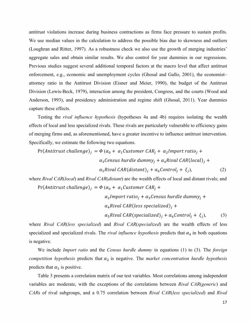
Testing the rival influence hypothesis (hypotheses 4a and 4b) requires isolating the wealth

effects of local and less specialized rivals. These rivals are particularly vulnerable to efficiency gains

of merging firms and, as aforementioned, have a greater incentive to influence antitrust intervention.

Specifically, we estimate the following two equations.

Pr #$%&%'()%+ℎ-../$0/ 1 = G(23 +256()%78/'6#91 +2:;8<7'%'-%&71 +

2=6/$)()ℎ('>./>(88?1 + 2@9&A-.6#9 .7+-. 1 +

2D9&A-.6#9(>&)%-$%)1 + 2H67$%'7.1 +I1), (2)

where Rival CAR(local) and Rival CAR(distant) are the wealth effects of local and distant rivals; and

Pr #$%&%'()%+ℎ-../$0/ 1 = G(23 +256()%78/'6#91 +

2:;8<7'%'-%&71 + 2=6/$)()ℎ('>./>(88?1 +

2@9&A-.6#9 ./)))</+&-.&J/> 1 +

2D9&A-.6#9()</+&-.&J/>)1 + 2H67$%'7.1 +I1), (3)

where Rival CAR(less specialized) and Rival CAR(specialized) are the wealth effects of less

specialized and specialized rivals. The rival influence hypothesis predicts that 2@ in both equations

is negative.

We include Import ratio and the Census hurdle dummy in equations (1) to (3). The foreign

competition hypothesis predicts that 2: is negative. The market concentration hurdle hypothesis

predicts that 2= is positive.

Table 3 presents a correlation matrix of our test variables. Most correlations among independent

variables are moderate, with the exceptions of the correlations between Rival CAR(generic) and

CARs of rival subgroups, and a 0.75 correlation between Rival CAR(less specialized) and Rival

18

CAR(distant). Since variation in Rival CAR(generic) is largely captured by the paired CARs of rival

subgroups, i.e., Rival CAR(less specialized) and Rival CAR(specialized), and Rival CAR(distant) and

Rival CAR(local), we do not include Rival CAR(generic) in equations (2) and (3). Similarly, the high

correlation between Rival CAR(less specialized) and Rival CAR(distant) is not a concern as they do

not appear in the same regression by design.

4.2 Endogeneity of measured wealth effects

An endogeneity issue potentially confounding the estimation is the simultaneity of case

selection and related firms’ wealth effects. Previous studies (Eckbo, Maksimovic, and Williams,

1990; Aktas, de Bodt, and Roll, 2004, 2007) show that investors can anticipate regulatory activities

and announcement wealth effects incorporate this anticipation. In other words, announcement

wealth effects reflect both the value consequences of a completed merger and the likelihood of

completion.

Similar to Aktas, de Bodt, and Roll (2007), we perform a two-step Rivers and Vuong (1988)

type test to check whether endogeneity is a concern in our Probit regressions. In a first step, we

instrument the wealth effects with exogenous variables that have no impact on antitrust intervention

other than through indirect impacts via the wealth effects. For Combined CAR, we select five

instruments, namely Surprise deal dummy, Tender offer dummy, Hostile takeover dummy, Industry-

adjusted stock payment percentage, and Bidder past performance. For the CARs of rival portfolios,

we employ three instruments, namely, Surprise deal dummy, Rival relative size, and Delaware

incorporation intensity. For the CARs of customer portfolios, we instrument using Surprise deal

dummy, Customer relative size, and Customer dependence. For brevity, Appendix 4 describes the

justification for each set of instruments in detail. In a second step, we add the residuals from the

first-stage to Eqs. (1)–(3). An insignificant coefficient on a residual indicates that endogeneity does

not significantly bias the un-instrumented probit estimates.

Column 3 of table 4, columns 3 and 8 of table 5, and column 3 of tables 6 and 7 report the

endogeneity test results. In table 4, panel A, the coefficient on the first-step regression residuals of

Customer CAR(local) is significant, rejecting the null of no endogeneity bias. Similarly, in panel B,

the coefficient on the first-step regression residuals of Customer CAR(reliant) also rejects the null of

no endogeneity bias. In addition, the endogeneity bias associated with Combined CAR is significant

in all specifications. In tables 5–7, these endogeneity bias patterns hold except in panel B of table 7,

where the endogeneity bias associated with Customer CAR(reliant) is insignificant.

19

We report the IV probit results in the adjacent columns to the endogeneity test results. In table 4,

we focus on examining the association between antitrust intervention and the wealth effects of

corporate customers. In table 5, we further isolate the wealth effects of sub-group rival CARs.

Following Aktas, de Bodt, and Roll (2007), when the bias of an endogenous variable is significant,

we substitute its fitted value from the first-stage regression in the second stage probit. Otherwise, we

keep the original variable and use its coefficient for statistical inference. For completeness,

Appendix 5 presents the first-step regression results. For comparison purposes, tables 4–7 report the

un-instrumented probit regression results in the columns before the endogeneity test results.

4.3 Testing the consumer protection hypothesis

In table 4, we focus on testing the consumer protection hypothesis (hypotheses 1a–1c). In panel

A, we examine the effect of Customer CAR(local) and Customer CAR(generic) in the regressions.

Although the probit regression in column 1 gives significant coefficients on both Customer

CAR(generic) and Customer CAR(local), this significance pattern changes in the IV probit

regression in column 4, which includes the actual values of Customer CAR(generic) and Rival

CAR(generic), and the fitted value of Customer CAR(local) and Combined CAR. The coefficient on

Customer CAR(local) is no longer significant and the coefficient on Customer CAR(generic) is not

significant at conventional levels. This result shows that antitrust intervention is not sensitive to the

wealth effect of either average customers or local customers, inconsistent with hypotheses 1a and 1c.

Table 4, panel B examines the effect of Customer CAR(reliant) and Customer CAR(generic). The IV

probit regression includes the actual values of Customer CAR(generic) and Rival CAR(generic), and

the fitted values of Customer CAR(reliant) and Combined CAR. The coefficients on Customer

CAR(reliant) and Customer CAR(generic) are both insignificant, inconsistent with hypotheses 1b

and 1c. The un-instrumented probit regression yields similar results. Taken together, these findings

show that the antitrust agencies are not systematically concerned about the anticompetitive impact

on customers geographically close to the merging firms or customers relying most on the input of

the merging firms. Furthermore, they fail to consider the impact on average customers of the

merging industry. Given that the wealth effects to local customers, generic customers, or more

reliant customers do not systematically affect antitrust case selection, when testing the remaining

three hypotheses (the foreign competition hypothesis, the market doctrine hypothesis, and the rival

influence hypothesis) in tables 5–7, we control for generic customer CAR only in our main

specifications (equations 2 and 3), and report the results in table 5. As a robustness check of

20

equations (2) and (3), we report the results of further controlling for local customer CAR in table 6

and for reliant customer CAR in table 7. We base our main interpretation of the three hypotheses on

table 5, referring to the results of tables 6 and 7 only when necessary.

4.4 Testing the foreign competition hypothesis

Turning to the foreign competition hypothesis (hypothesis 2), Import ratio consistently has a

negative coefficient across the specifications in tables 4–7 (significant at 1% in all specifications).

For example, in table 5, column 5, equation (2), the marginal effect of Import ratio is −0.900,

indicating that a 10% increase in Import ratio reduces the likelihood of an antitrust challenge by 9%.

A one standard deviation increase in Import Ratio leads to around a 6% decrease in the probability

of antitrust intervention. Equation (3) gives a similar result for the effect of foreign competition. The

marginal effect of Import ratio is −0.910 (table 5, column 10), suggesting that a one standard

deviation increase in Import Ratio leads to around a 6.7% decrease in the probability of antitrust

intervention.17 This result is consistent with the foreign competition hypothesis. It also echoes the

argument of Mitchell and Mulherin (1996) that foreign competition makes an industry more difficult

to monopolize and stimulates domestic companies to merge to improve efficiency.

4.5 Testing the market concentration hurdle hypothesis

We obtain results clearly consistent with the market concentration hurdle hypothesis

(hypothesis 3) in the main specification in tables 4 and 5. On average, hitting the market

concentration hurdle leads to an immediate increase in the probability of intervention of 18% (table

5, column 5, equation 2) to 19% (table 5, column 10, equation 3). The robustness test results in

tables 6 and 7 are mixed: in table 6, the coefficient on Census hurdle dummy is insignificant in the

IV probit, while in table 7 Census hurdle dummy has a positive coefficient in both the un-

instrumented and IV probits. Overall in tables 4–7, however, Census hurdle dummy has an

insignificant coefficient in only two out of eight IV probit specifications. The results

overwhelmingly support the market concentration hurdle hypothesis.

We note that academics have been doubtful of the antitrust agencies' heavy reliance on industry

concentration. Aktas, de Bodt, and Roll (2007) assert that “The problem, of course, is that the theory

behind the ex-ante approach is deeply flawed. As is well known, one can generate a positive

relationship between industry concentration and profitability either via a competitive scale-17Across all the specifications in tables 6 and 7, the effect of foreign competition remains fairly stable: A one standard deviation increase in Import Ratio leads to around a 5−8% decrease in the probability of antitrust intervention.

21

economies argument, or via a monopoly argument” (Aktas, de Bodt, and Roll, 2007, p.1118). Eckbo

(1992) also concludes that “the evidence systematically rejects the antitrust doctrine even for values

of industry concentration and market shares which, over the past four decades, have been considered

crucial in determining the probability that a horizontal merger will have anticompetitive effects”

(Eckbo, 1992, p.1028). But, as it is difficult to verify the anticompetitive effect of a horizontal

merger (especially before deal completion), it can be costly to precisely identify harmful cases.

Reliance on market concentration criteria can be a rational choice by resource constrained antitrust

agencies. Wood and Anderson’s (1993) survey refers to several resource constraints that antitrust

agencies face, including limited budgets and shortages of economists and attorney professionals.

This probably explains why, despite heavily criticism of its oversimplification, market concentration

remains central to antitrust enforcement.

4.6 Testing the rival influence hypothesis

In tables 5–7, we test the rival influence hypothesis (hypotheses 4a and 4b). Local rivals and

less specialized rivals are most likely to be negatively affected by merger efficiency gains. These

rivals are therefore most incentivized to incur the costs of influencing antitrust intervention in their

favor. In table 5, we add Rival CAR(local) and Rival CAR(distant) to the regressions in columns 1–5,

and add Rival CAR(less specialized) and Rival CAR(specialized) to the regressions in columns 6–10,

while controlling for the average wealth effect to downstream customers. For robustness, we further

control for the wealth effect to local customers and reliant customers, and report these robustness

results for Rival CAR(local) and Rival CAR(distant) in table 6, and for Rival CAR(less specialized)

and Rival CAR(specialized) in table 7. As section 4.1 explains, since variation in Rival CAR(generic)

is largely captured by the twin CARs of rival subgroups, we exclude Rival CAR(generic) from

equations (2) and (3).18

The endogeneity test in table 5 column 3 shows that Rival CAR(local) and Rival CAR(distant)

have insignificant endogeneity biases. We therefore include their actual values in the IV probit in

column 4. The coefficient on Rival CAR(local) is −10.995 (z = −3.44). The marginal effect indicates

that a 10% decrease in Rival CAR(local) leads to an increase of 14% in the probability of antitrust

intervention. In contrast, Rival CAR(distant) has a coefficient of 10.699 (z = 1.70), insignificant at

conventional levels. An interpretation of this insignificant coefficient is that competitive pressure 18Including the residuals from a regression of Rival CAR(generic) on Rival CAR(local) in equation (2), and the residuals from a regression of Rival CAR(generic) on Rival CAR(less specialized) in equation (3) leaves the reported results unchanged.

22

due to merging firms’ efficiency gains are less likely to affect distant rivals, so they have less

incentive to influence intervention. For completeness, we report the un-instrumented probit results

in columns 1 and 2. The results are qualitatively similar and the magnitudes of the marginal effects

are close to those of the IV probit. The robustness tests in table 6 further confirm our findings. The

coefficient on Rival CAR(local) is −9.110 (z = −2.42) in panel A and −12.081 (z = −3.08) in panel B,

both significant at 5% or better.

The endogeneity test in table 5 column 8 shows that Rival CAR(less specialized) and Rival

CAR(specialized) have insignificant endogeneity biases. Therefore, we include their actual values in

the IV probit in column 9. In the IV probit regression, Rival CAR(less specialized) has a negative

coefficient of −11.220 (z = −1.99). The marginal effect suggests that a 10% decrease in Rival

CAR(less specialized) leads to a 14% increase in the likelihood of a case being challenged. Rival

CAR(specialized) has an insignificant coefficient. This is consistent with specialized rivals being

better protected from the negative impact of merging firms’ efficiency gain, and therefore having

less incentive to influence intervention. The robustness test results are mixed: the coefficient on

Rival CAR(less specialized) is −12.402 (z = −2.91) in table 7 panel A (when further controlling for

the local customer wealth effect), confirming the possible influence of less specialized industry

competitors on antitrust intervention. The coefficient on Rival CAR(less specialized), however, turns

insignificant in table 7 panel B (when further controlling for the reliant customer wealth effect).

Overall, in table 5 and table 7, Rival CAR(less specialized) has a significant coefficient in two out of

three IV probit specifications, supporting the hypothesis that less specialized industry rivals

influence antitrust intervention.

In sum, tables 5–7 provide evidence of greater antitrust protection of most affected rivals. These

industry rivals are likely to promote this protection, which is not necessarily socially efficient. This

finding differs from that of Duso, Neven, and Röller (2007). Their analysis of European merger

control suggests that the European Commission’s decisions are not sensitive to firms’ interests,

including those of industry competitors. As we discuss earlier, there are various ways that concerned

rivals can influence the antitrust agencies. For example, local rivals can form a local trade

association to exert direct pressure on antitrust agencies, lobby against the deal, or exert indirect

influence through campaign contributions (McChesney, 1997) or quid pro quo deals (Tahoun, 2014).

Our evidence is consistent with Bittlingmayer and Hazlett’s (2000, p.351) observation on the

Microsoft antitrust case that, “The May 1998 suit filed by the DOJ was accompanied by a suit filed

23

by 20 states. As has been widely observed in the press, these states appear to have been the subject

of intense lobbying pressure from locally based computer companies”. Our evidence also echoes

Posner (1969), who asserts that the FTC’s antitrust activities face pressure from Congress, and their

investigations are initiated “at the behest of corporations, trade associations, and trade unions whose

motivation is at best to shift the costs of their private litigation to the taxpayer and at worst to harass

competitors” (Posner, 1969, p.88).

We also obtain some meaningful results for the coefficients on several control variables. The

coefficient on Combined CAR is consistently negative in the IV probit regressions in tables 4–7, and

significant at conventional levels in most specifications. This suggests a possibility of merging firms

influencing the antitrust agencies to clear deals. The coefficient on Relative deal size is consistently

positive in the IV probit regressions in tables 4–7, suggesting that antitrust agencies consider the

deal’s importance to the bidder as an indicator of merger motives. Furthermore, antitrust

intervention is positively related to Ln Bidder market cap in most specifications, suggesting that

deals from larger bidders are more likely to be challenged. Antitrust agencies may believe that large

bidders are more likely to have a greater impact on public interest or will attract more public

attention. In addition, the coefficient on Industry growth is insignificant in all specifications. This

differs from the countercyclical antitrust litigation argument of Ghosal and Gallo (2001) and from

Amacher, Higgins, Shughart, and Tollison’s (1985) story of regulators cushioning producer losses in

bad times. This may be due to the existence of both effects offsetting in the net effect.

4.7 Weak instruments

Appendix 5 reports the first step OLS regressions of the IV probit procedure, columns 1–3 for

the wealth effect to customer portfolios, columns 4–8 for the wealth effect to rival portfolios, and

column 9 for the combined CAR. The R2s of all first-step OLS regressions are reasonable, being

0.21 for Combined CAR, and 0.09 and above for customer and rival CARs. For Customer

CAR(local), Customer CAR(reliant), and Combined CAR, a Fisher test rejects the null hypothesis

that all selected exogenous variable coefficients are zero, suggesting our instruments for the wealth

effect of local and reliant customers, and merging firms are not weak. The results for generic

customer CAR and all rival portfolio CARs are not as good. These estimates are in line with Aktas,

de Bodt, and Roll (2007), who identify the source of the weak instrument difficulty to be noisy

cumulative abnormal returns. For robustness, we follow Aktas, de Bodt, and Roll (2007) and use a

modified version of Anderson and Rubin’s (1949) procedure to check whether the inferences from

24

our previous tests are valid. The OLS regressions in the first step remain unchanged, but a linear

probability model replaces the probit regressions in the second step, with p-values estimated by a

percentile-t bootstrap (with 2,500 replications) replacing robust p-values.19 The test results remain

qualitatively the same as in tables 4 and 5 with two exceptions: first, the significance of the

coefficient on Rival CAR(less specialized) falls to 10% in table 5; second, the coefficient on

Combined CAR turns insignificant in both panels of table 4 and falls to 10% significance in table 5.

Therefore, although some of our instruments are weak, this robustness check indicates that they are

still strong enough to support meaningful inference.

5. Summary and concluding remarks

What determines antitrust intervention in horizontal mergers? In this paper, we model the

decision process of antitrust intervention at the deal level. We formulate four hypotheses based on

economic theories and previous literature: the consumer protection hypothesis, the foreign

competition hypothesis, the market concentration hurdle hypothesis, and the rival influence

hypothesis. We test these hypotheses using a sample of horizontal mergers in the U.S.

manufacturing sector announced between 1980 and 2009.

Our results suggest both efficiency and inefficiency in the antitrust intervention process. On the

inefficiency side, we find that antitrust enforcement is not consistent with the stated aim of

consumer protection. Antitrust agencies do not systematically respond to the wealth effects of

customers in general, nor to the wealth effects of local customers or customers in the most reliant

downstream industry. We also observe evidence consistent with the hypothesis that certain

concerned rival groups can influence antitrust intervention in their favor. These rivals are local and

less specialized rivals who are most likely to face pressure from the efficiency gains of merging

firms. Our results on rival influence also enrich our understanding of the sources of demand for

regulation (Stigler, 1971). On the efficiency side, our results show that, consistent with the foreign

competition hypothesis, the likelihood of antitrust intervention decreases with foreign import

competition, suggesting that the antitrust agencies are less likely to expend resources to challenge

areas where supply elasticity is high, the industry is difficult to monopolize, and mergers are more

likely to be motivated by efficiency gains rather than anticompetitive rents. This finding also

19According to Wooldridge (2002), this procedure approximates the second step qualitative dependent model and generates robust estimates.

25

highlights the importance of maintaining an open market to contain the detrimental consequence of

monopolization on consumers. We also find evidence for the market concentration hurdle

hypothesis, suggesting that the authorities effectively implement the concentration hurdle rules

contained in the Horizontal Merger Guidelines. The prior literature provides no evidence on the

determinants of antitrust intervention at the deal level. Our study fills this gap. Our findings can be a

useful reference for calibrating the efficiency of antitrust regulation and enforcement.

26

References

Agrawal, A., Jaffe, J.F., 2000. The post-merger performance puzzle. Advances in Mergers and

Acquisitions 1, 7–41.

Ahern, K.R., 2012. Bargaining power and industry dependence in mergers. Journal of Financial

Economics 103, 530–550.

Ali, A., Klasa, S., Yeung, E., 2009. The limitations of industry concentration measures

constructed with Compustat data: implications for finance research. Review of Financial

Studies 22, 3839–3871.

Aktas, N., de Bodt, E., Roll, R., 2004. Market response to European regulation of business

combinations. Journal of Financial and Quantitative Analysis 39, 731–757.

Aktas, N., de Bodt, E., Roll, R., 2007. Is European M&A regulation protectionist? Economic

Journal 117, 1096–1211.

Amacher, R.C., Higgins, R.S., Shughart II, W.F., Tollison, R.D., 1985. The behavior of

regulatory activity over the business cycle: An empirical test. Economic Inquiry 23, 7–19.

Baron, D., 1998. Integrated market and nonmarket strategies in client and interest group politics.

Stanford Graduate School of Business Working Paper.

Baumol, W., Ordover, J., 1985. Use of antitrust to subvert competition. Journal of Law and

Economics 28, 247–266.

Becher, D.A., Mulherin, J.H., Walkling, R.A., 2012. Sources of gains in corporate mergers:

Refined tests from a neglected industry. Journal of Financial and Quantitative Analysis 47,

57–89.

Bhattacharyya, S., Nain, A., 2011. Horizontal acquisitions and buying power: A product market

analysis. Journal of Financial Economics 99, 97–115.

Bittlingmayer, G., Hazlett, T.W., 2000. DOS Kapital: Has antitrust action against Microsoft

created value in the computer industry? Journal of Financial Economics 55, 329–359.

Block, M.K., Feinstein, J.S., 1986. The spillover effect of antitrust enforcement. The Review of

Economics and Statistics 68, 122–31.

Bradley, M., Desai, A., Kim, E., 1988. Synergistic gains from corporate acquisitions and their

division between the stockholders of target and acquiring firms. Journal of Financial

Economics 21, 3–40.

27

Bruner, R.F., 2004. Applied Mergers and Acquisitions (University edition). Wiley Finance: New

Jersey.

Cournot, A.A., [1838] 1927. Researches into the Mathematical Principles of the Theory of

Wealth. Macmillan: New York.

Duso, T., 2005. Lobbying and regulation in a political economy: Evidence from the U.S. Cellular

Industry. Public Choice 122, 251–276.

Duso, T., Neven, D.J., Röller, L., 2007. The Political economy of European merger control:

Evidence using stock market data. Journal of Law and Economics 50, 455–489.

Duso, T., Gugler, K., Yurtoglu, B.B., 2011. How effective is European merger control. European

Economic Review 55, 980–1006.

Eckbo, B.E., 1983. Horizontal mergers, collusion, and stockholder wealth. Journal of Financial

Economics 11, 241–271.

Eckbo, B.E., 1985. Mergers and the Market Concentration Doctrine: Evidence from the capital

market. The Journal of Business 58, 325–349.

Eckbo, B.E., Wier, P., 1985. Antimerger policy under the Hart-Scott-Rodino Act: A re-

examination of the market power hypothesis. Journal of Law and Economics 28, 119–149.

Eckbo, B.E., 1988. Competition and wealth effects of mergers. In F. Mathewson, M. Trebilcock

and M. Walker, eds. (1990): The Law and Economics of Competition Policy, chapter 9,

297–332. The Fraser Institute: Vancouver.

Eckbo, B.E., 1992. Mergers and the value of antitrust deterrence. Journal of Finance 47, 1005–

1029.

Eckbo, E., Maksimovic, V., Williams, J., 1990. Consistent estimation of cross-sectional models

in event studies. Review of Financial Studies 3, 343–65.

Eckbo, B.E., Makaew, T., Thorburn, K.S., 2014. Are stock-financed takeovers opportunistic?

Tuck at Dartmouth Working Paper.

Eisner, M.A., Meier, K.J., 1990. Presidential control versus bureaucratic power: Explaining the

Reagan revolution in antitrust. American Journal of Political Science 34, 269–87.

Ellert, J.C., 1976. Mergers, antitrust law enforcement and stockholder returns. Journal of

Finance 31, 715–732.

Fan, J.P.H., Lang, L.H.P., 2000. The measurement of relatedness: an application to corporate

diversification. Journal of Business 73, 629–660.

28

Fee, C.E., Thomas, S., 2004. Sources of gains in horizontal mergers: evidence from customer,

supplier, and rival firms. Journal of Financial Economics 74, 423–460.

Feinberg, R.M., Reynolds, K.M., 2010. The determinants of state-level antitrust activity. Review

of Industrial Organization 37, 179–196.

Gaughan, P.A., 2015. Mergers, Acquisitions, and Corporate Restructurings. Wiley: New Jersey.

Ghosal, V., and Gallo, J., 2001. The cyclical behaviour of the Department of Justice’s antitrust

enforcement activity. International Journal of Industrial Organization 19, 27–54.

Ghosal, V., 2011. Regime shift in antitrust laws, economics and enforcement. Journal of

Competition Law and Economics 7, 733–774.

Giroud, X., Mueller, H., 2010. Does corporate governance matter in competitive industries?

Journal of Financial Economics 95, 312–331.

Greene, W.H., 2003. Econometric Analysis. Upper Saddle River, NJ: Prentice Hall.

Hansen, R., 1987. A theory for the choice of exchange medium in mergers and acquisitions.

Journal of Business 60, 75–95.

Hoberg, G., Phillips, G., 2016. Text-based network industries and endogenous product

differentiation. Journal of Political Economy 124, 1423–1465.

Ivanov, V., Joseph, K., Wintoki, M.B., 2013. Disentangling the market value of customer

satisfaction: Evidence from market reaction to the unanticipated component of ACSI

announcements. International Journal of Research in Marketing 30, 168–178.

Johnson, R.N., Parkman, A.M., 1991. Premerger notification and the incentive to merge and

litigate. Journal of Law, Economics, & Organization 7, 145–162.

Kale, J.R., Shahrur, H.K., 2007. Corporate capital structure and the characteristics of suppliers

and customers. Journal of Financial Economics 83, 321–365.

Katics, M.M., Petersen, B.C., 1994. The effect of rising import competition on market power: A

panel data study of US manufacturing. Journal of Industrial Economics 42, 277–286.

Klasa, S., Ortiz-Molina, H., Serfling, M.A., Srinivasan, S., 2017. Protection of trade secrets and

capital structure decisions. Working Paper.

Long, W.F., Schramm, R., Tollison, R., 1973. The economic determinants of antitrust activity.

Journal of Law and Economics 16, 351–363.

Loughran, T., Ritter, J., 1997. The operating performance of firms conducting seasoned equity

offerings. Journal of Finance 52, 1823–1850.

29

McChesney, F., 1997. Money for Nothing: Politicians, Rent Extraction, and Political Extortion.

Harvard University Press: Cambridge.

Mitchell, M.L., Mulherin, J.H., 1996. The impact of industry shocks on takeover and

restructuring activity. Journal of Financial Economics 41, 193–229.

Nash, J.F., 1950. Equilibrium points in N-person games. Proceedings of the National Academy

of Sciences of the U.S.A. 36, 48–49.

Pigou, A.C., 1932. The Economics of Welfare (4th ed.). Macmillan: London.

Posner, R.A., 1969. The federal trade commission. University of Chicago Law Review 37, 47–89.

Posner, R.A., 2013. The concept of regulatory capture: a short, inglorious history. In D.

Carpenter and D.A. Moss (eds), Preventing Regulatory Capture: Special Interest Influence

and How to Limit it. New York: Cambridge University Press, 49–56.

Rhodes-Kropf, M., Robinson, D.T., Viswanathan, S., 2005. Valuation waves and merger activity:

The empirical evidence. Journal of Financial Economics 77, 561–603.

Rivers, D., Vuong, Q.H., 1988. Limited information estimators and exogeneity tests for

simultaneous probit models. Journal of Econometrics 39, 347–366.

Rogowsky, R.A., 1982. An economic study of anti-merger remedies. PhD dissertation,

University of Virginia.

Schwert, G.W., 2000. Hostility in takeovers: In the eyes of the beholder. Journal of Finance 55,

2599–2640.

Shahrur, H., 2005. Industry structure and horizontal takeovers: Analysis of wealth effects on

rivals, suppliers, and corporate customers. Journal of Financial Economics 76, 61–98.

Shaked, A., Sutton, J., 1987. Product differentiation and industrial structure. Journal of

Industrial Economics 26, 131–146.

Shivdasani, A., 1993. Board composition, ownership structure, and hostile takeovers. Journal of

Accounting and Economics 16, 167–198.

Shleifer, A., Vishny, R.W., 2003. Stock market driven acquisitions. Journal of Financial

Economics 70, 295–311.

Slovin, M.B., Sushka, M.E., Hudson, C.D., 1991. Deregulation, contestability, and airline

acquisitions. Journal of Financial Economics 30, 231–251.

Song, M.H., Walkling, R.A., 2000. Abnormal returns to rivals of acquisition targets: A test of the

“acquisition probability hypothesis”. Journal of Financial Economics 55, 143–171.

30

Stigler, G.J., 1964. A theory of oligopoly. Journal of Political Economy 72, 44–61.

Stigler, G.J., 1968. The Organization of Industry. University of Chicago Press: Chicago.

Stigler, G.J., 1971. The theory of economic regulation. Bell Journal of Economics 2, 3–21.

Stillman, R., 1983. Examining antitrust policy towards horizontal mergers. Journal of Financial

Economics 11, 225–240.

Streitwieser, M.R., September 2010. Measuring the nation’s economy: An industry perspective,

a primer on BEA’s industry accounts. Bureau of Economic Analysis.

http://www.bea.gov/industry/pdf/industry_primer.pdf.

Sutton, J., 1991. Sunk Costs and Market Structure. MIT Press: Cambridge.

Tahoun, A., 2014. The role of stock ownership by US members of Congress on the market for

political favors. Journal of Financial Economics 111, 86–110.

Travlos, N.G., 1987. Corporate takeover bids, methods of payment and bidding firms’ stock

returns. Journal of Finance 42, 943–963.

Valta, P., 2012. Competition and the cost of debt. Journal of Financial Economics 105, 661–682.

Wier, P., 1983. The costs of antimerger lawsuits: Evidence from the stock market. Journal of

Financial Economics 11, 207–224.

Wood, B.D., Anderson, J.E., 1993. The politics of U.S. antitrust regulation. American Journal of

Political Science 37, 1–39.

Wooldridge, J.M., 2002. Econometric Analysis of Cross Section and Panel Data. The MIT Press.

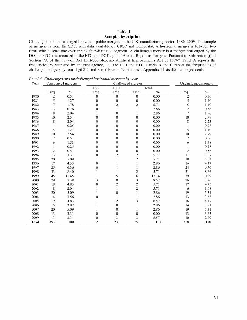
31

Table 1 Sample description

Challenged and unchallenged horizontal public mergers in the U.S. manufacturing sector, 1980–2009. The sample of mergers is from the SDC, with data available on CRSP and Compustat. A horizontal merger is between two firms with at least one overlapping four-digit SIC segment. A challenged merger is a merger challenged by the DOJ or FTC, and recorded in the FTC and DOJ’s joint “Annual Report to Congress Pursuant to Subsection (j) of Section 7A of the Clayton Act Hart-Scott-Rodino Antitrust Improvements Act of 1976”. Panel A reports the frequencies by year and by antitrust agency, i.e., the DOJ and FTC. Panels B and C report the frequencies of challenged mergers by four-digit SIC and Fama–French 49 industries. Appendix 1 lists the challenged deals. Panel A: Challenged and unchallenged horizontal mergers by year

Year Announced mergers Challenged mergers Unchallenged mergers DOJ FTC Total Freq. % Freq. Freq. Freq. % Freq. %

1980 2 0.51 0 0 0 0.00 2 0.56 1981 5 1.27 0 0 0 0.00 5 1.40 1982 7 1.78 0 2 2 5.71 5 1.40 1983 3 0.76 0 1 1 2.86 2 0.56 1984 8 2.04 1 0 1 2.86 7 1.96 1985 10 2.54 0 0 0 0.00 10 2.79 1986 8 2.04 0 0 0 0.00 8 2.23 1987 1 0.25 0 0 0 0.00 1 0.28 1988 5 1.27 0 0 0 0.00 5 1.40 1989 10 2.54 0 0 0 0.00 10 2.79 1990 2 0.51 0 0 0 0.00 2 0.56 1991 6 1.53 0 0 0 0.00 6 1.68 1992 1 0.25 0 0 0 0.00 1 0.28 1993 2 0.51 0 0 0 0.00 2 0.56 1994 13 3.31 0 2 2 5.71 11 3.07 1995 20 5.09 1 1 2 5.71 18 5.03 1996 17 4.33 0 1 1 2.86 16 4.47 1997 25 6.36 0 1 1 2.86 24 6.70 1998 33 8.40 1 1 2 5.71 31 8.66 1999 45 11.45 1 5 6 17.14 39 10.89 2000 29 7.38 3 0 3 8.57 26 7.26 2001 19 4.83 0 2 2 5.71 17 4.75 2002 8 2.04 1 1 2 5.71 6 1.68 2003 20 5.09 1 0 1 2.86 19 5.31 2004 14 3.56 0 1 1 2.86 13 3.63 2005 19 4.83 1 2 3 8.57 16 4.47 2006 15 3.82 1 0 1 2.86 14 3.91 2007 20 5.09 1 0 1 2.86 19 5.31 2008 13 3.31 0 0 0 0.00 13 3.63 2009 13 3.31 0 3 3 8.57 10 2.79 Total 393 100 12 23 35 100 358 100

32

Table 1 (continued)

Panel B: Challenged horizontal merger distribution by SIC industry SIC SIC Industry Freq. % 2011 Meat Packing Plants 1 2.86 2026 Fluid Milk 1 2.86 2041 Flour and Other Grain Mill Products 1 2.86 2051 Bread and Other Bakery Products, Except Cookies and Crackers 1 2.86 2621 Paper Mills 1 2.86 2834 Pharmaceutical Preparations 9 25.71 2836 Biological Products, Except Diagnostic Substances 1 2.86 2844 Perfumes, Cosmetics, and Other Toilet Preparations 1 2.86 2851 Paints, Varnishes, Lacquers, Enamels, and Allied Products 1 2.86 2869 Industrial Organic Chemicals, Not Elsewhere Classified 1 2.86 2873 Nitrogenous Fertilizers 1 2.86 2899 Chemicals and Chemical Preparations, Not Elsewhere Classified 1 2.86 2911 Petroleum Refining 3 8.57 3312 Steel Works, Blast Furnaces & Rolling Mills (Coke Ovens) 1 2.86 3357 Drawing and Insulating of Nonferrous Wire 1 2.86 3674 Semiconductors and Related Devices 1 2.86 3728 Aircraft Parts and Auxiliary Equipment, Not Elsewhere Classified 1 2.86 3731 Ship Building and Repairing 3 8.57 3812 Search, Detection, Navigation, Guidance, Aeronautical, and Nautical

Systems and Instruments 2 5.71

3841 Surgical and Medical Instruments and Apparatus 2 5.71 3845 Electromedical and Electrotherapeutic Apparatus 1 2.86 Total 35 100 Panel C: Challenged horizontal merger distribution by Fama–French 49 industries Fama–French 49 industries Freq. % Pharmaceutical Products 10 28.57 Chemicals 4 11.43 Food Products 4 11.43 Electronic Equipment 3 8.57 Medical Equipment 3 8.57 Petroleum and Natural Gas 3 8.57 Shipbuilding, Railroad Equipment 3 8.57 Steel Works Etc. 2 5.71 Aircraft 1 2.86 Consumer Goods 1 2.86 Business Supplies 1 2.86 Total 35 100

33

Table 2 Descriptive statistics

Summary statistics of variables in the regression analysis. Panel A reports abnormal returns to the combined firms, rivals, and customers in challenged and unchallenged horizontal mergers during 1980–2009. Panel B reports the summary statistics of other variables in the regression analysis. Appendix 3 defines all variables. Data are from the Bureau of Economic Analysis (BEA) IO accounts, SDC and Compustat consolidated and industry-segment tapes. The t-statistics in parentheses are based on a test for the equality of means. A t-test (Ranksum test) tests mean (median) differences of the continuous variables between challenged and unchallenged deals. A Pearson K: test tests dummy variable frequency differences between challenged and unchallenged deals. *, **, and *** denote significance at 10%, 5%, and 1%. Panel A: Abnormal returns to the combined firms, rivals, and customersFirm portfolio Overall sample Challenged mergers Unchallenged mergers Mean diff.

Mean (%) N Mean (%) N Mean (%) N (t-stat) Merging firms Combined firms 2.015*** 393 1.580*** 35 2.057*** 358 0.477

(4.64) (1.32) (4.45) (0.31) Bidder −2.587*** 393 −3.847*** 35 −2.463*** 358 1.383

(−5.67) (−3.12) (−5.07) (0.86) Target 23.144*** 393 18.395*** 35 23.608*** 358 5.213

(18.08) (4.80) (17.45) (1.16)

Rivals Rivals (generic) 0.382*** 393 0.289 35 0.392*** 358 0.102

(3.42) (0.85) (3.31) (0.26) Rivals (local) 0.503*** 393 0.038 34 0.549*** 349 0.511

(3.31) (0.09) (3.38) (0.95) Rivals (distant) 0.376*** 393 0.601 34 0.355*** 358 −0.246

(3.02) (1.60) (2.69) (−0.56) Rivals (less specialized) 0.350*** 393 0.101 35 0.374*** 357 0.273

(2.94) (0.29) (2.97) (0.65) Rivals (specialized) 0.426** 393 0.810* 35 0.388** 358 −0.422

(2.57) (1.84) (2.20) (−0.73)

Customers Customers (generic) 0.244** 393 0.859** 35 0.183 358 −0.676*

(2.16) (2.07) (1.57) (−1.71) Customers (local) −0.098 374 −0.273 33 −0.081 341 0.192

(−0.69) (−0.65) (−0.54) (0.38) Customers (reliant) 0.236 284 0.021 25 0.257 259 0.236

(0.82) (0.02) (0.85) (0.23)

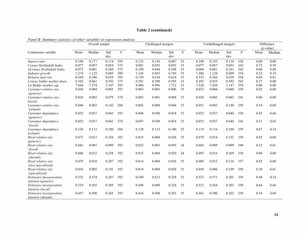
34

Table 2 (continued)

Panel B: Summary statistics of other variables in regression analysis Overall sample Challenged mergers Unchallenged mergers Difference

(p-value) Continuous variable Mean Median Std.

dev. N Mean Median Std.

dev. N Mean Median Std.

dev. N Mean

Median

Import ratio 0.184 0.177 0.114 393 0.125 0.136 0.087 35 0.190 0.193 0.114 358 0.00 0.00 Census Herfindahl Index 0.077 0.057 0.054 375 0.081 0.055 0.055 33 0.077 0.057 0.053 342 0.73 0.58 ∆Census Herfindahl Index 0.072 0.001 0.260 375 0.199 0.044 0.398 33 0.060 0.001 0.241 342 0.00 0.00 Industry growth 1.274 1.125 0.805 389 1.145 0.883 0.769 35 1.286 1.128 0.809 354 0.32 0.19 Relative deal size 0.569 0.396 0.629 393 0.739 0.610 0.624 35 0.553 0.366 0.628 358 0.09 0.01 Census bidder market share 0.302 0.061 0.593 375 0.391 0.208 0.595 33 0.293 0.053 0.592 342 0.37 0.00 Ln Bidder market cap 7.644 7.574 2.147 393 8.906 8.996 1.712 35 7.520 7.438 2.147 358 0.00 0.00 Customer relative size (generic)

0.030 0.004 0.085 393 0.003 0.001 0.006 35 0.033 0.004 0.088 358 0.05 0.00

Customer relative size (local)

0.026 0.002 0.079 374 0.002 0.001 0.004 33 0.028 0.003 0.082 341 0.06 0.00

Customer relative size (reliant)

0.046 0.003 0.142 284 0.002 0.000 0.004 25 0.051 0.003 0.148 259 0.10 0.00

Customer dependence (generic)

0.052 0.037 0.043 393 0.046 0.030 0.034 35 0.052 0.037 0.044 358 0.45 0.66

Customer dependence (local)

0.052 0.037 0.043 374 0.047 0.030 0.034 33 0.053 0.037 0.044 341 0.51 0.65

Customer dependence (reliant)

0.120 0.112 0.100 284 0.128 0.133 0.100 25 0.119 0.116 0.100 259 0.67 0.34

Rival relative size (generic)

0.073 0.013 0.184 393 0.015 0.004 0.028 35 0.079 0.014 0.191 358 0.05 0.00

Rival relative size (local)

0.043 0.007 0.099 383 0.023 0.003 0.095 34 0.045 0.009 0.099 349 0.22 0.01

Rival relative size (distant)

0.088 0.012 0.258 392 0.015 0.004 0.029 34 0.095 0.014 0.269 358 0.08 0.00

Rival relative size (less specialized)

0.079 0.010 0.207 392 0.014 0.004 0.028 35 0.085 0.012 0.216 357 0.05 0.00

Rival relative size (specialized)

0.054 0.005 0.191 393 0.014 0.004 0.028 35 0.058 0.006 0.199 358 0.20 0.01

Delaware incorporation intensity (generic)

0.525 0.574 0.207 393 0.549 0.612 0.258 35 0.523 0.571 0.201 358 0.48 0.34

Delaware incorporation intensity (local)

0.519 0.565 0.305 393 0.498 0.600 0.326 35 0.521 0.564 0.303 358 0.66 0.66

Delaware incorporation intensity (distant)

0.457 0.500 0.265 393 0.416 0.500 0.291 35 0.461 0.500 0.262 358 0.34 0.69

35

Table 2 (continued)

Overall sample Challenged mergers Unchallenged mergers Difference (p-value)

Continuous variable Mean Median Std. dev.

N Mean Median Std. dev.

N Mean Median Std. dev.

N Mean

Median

Delaware incorporation intensity (less specialized)

0.490 0.545 0.238 393 0.446 0.523 0.277 35 0.494 0.548 0.234 358 0.26 0.40

Delaware incorporation intensity (specialized)

0.526 0.625 0.324 393 0.617 0.750 0.368 35 0.517 0.614 0.318 358 0.08 0.03

Industry-adjusted stock payment percentage

0.001 0.000 0.023 393 –0.001 0.000 0.008 35 0.001 0.000 0.024 358 0.52 0.38

Bidder past performance 0.132 0.146 0.133 393 0.168 0.164 0.083 35 0.129 0.144 0.136 358 0.10 0.15 Overall sample Challenged mergers Unchallenged mergers Mean Diff.

Dummy variable Mean (%) N Mean (%) N Mean (%) N (p-value) Census hurdle dummy 7.20 27 24.24 8 5.56 19 0.00 Surprise deal dummy 46.82 184 40.00 14 47.49 170 0.40 Tender offer dummy 29.77 117 20.00 7 30.73 119 0.19 Hostile takeover dummy 5.85 23 8.57 3 5.59 20 0.47

36

Table 3 Correlation coefficients

Correlation matrix for all variables in the main regression models. Appendix 3 gives the definition of all variables. Customer

CAR (generic)

Customer CAR

(local)

Customer CAR

(reliant)

Rival CAR

(generic)

Rival CAR

(local)

Rival CAR

(distant)

Rival CAR

(less specialized)

Rival CAR

(specialized)Antitrust challenge 0.084 −0.022 0.013 −0.007 −0.020 0.012 −0.046 0.061 Customer CAR (generic) 0.674 0.347 0.246 0.227 0.169 0.155 0.173 Customer CAR (local) 0.284 0.215 0.211 0.129 0.150 0.152 Customer CAR (reliant) 0.122 0.156 0.073 0.066 0.089 Rival CAR (generic) 0.776 0.817 0.884 0.696 Rival CAR (local) 0.375 0.653 0.562 Rival CAR (distant) 0.751 0.569 Rival CAR (less specialized) 0.274

Combined CAR Import ratio Census hurdle dummy

Industry growth

Relative deal size

Census bidder market share

Ln bidder market cap

Antitrust challenge 0.007 −0.021 0.205 −0.049 0.047 0.047 0.199 Customer CAR (generic) 0.069 0.043 −0.018 0.033 0.007 0.111 0.008 Customer CAR (local) 0.023 −0.059 −0.026 0.038 0.012 0.044 −0.029 Customer CAR (reliant) 0.068 0.013 0.091 −0.025 0.039 0.029 0.009 Rival CAR (generic) 0.222 −0.039 0.018 0.075 0.006 0.027 0.025 Rival CAR (local) 0.170 −0.067 −0.022 0.066 −0.006 0.001 0.022 Rival CAR (distant) 0.183 −0.027 0.033 0.065 0.006 0.061 0.015 Rival CAR (less specialized) 0.223 −0.034 0.029 0.046 −0.004 0.026 0.013 Rival CAR (specialized) 0.088 −0.037 −0.023 0.033 0.003 −0.024 0.006 Combined CAR −0.080 0.060 −0.006 0.191 −0.004 −0.117 Import ratio −0.119 −0.049 −0.004 −0.044 0.121 Census hurdle dummy −0.005 0.027 0.127 0.083 Industry growth −0.037 0.034 −0.038 Relative deal size −0.208 −0.366 Census bidder market share 0.472

37

Table 4 The impacts of customer wealth effect, foreign competition, and market concentration hurdle on

antitrust case selectionThis table reports the impacts of customer wealth effect, foreign competition, and market concentration hurdle on antitrust case selection. Panel A focuses on the wealth effect impact of local customers, panel B on the wealth effect impact of reliant customers. In both panels, columns 1 and 2 report coefficients and marginal effects of un-instrumented probit regressions. Column 3 reports Rivers and Vuong (1988) endogeneity tests of wealth effect variables. Columns 4 and 5 report coefficients and marginal effects of two-step instrumental variable probit regressions. Residuals and fitted values are from the first-step OLS regressions in Appendix 5. Appendix 3 defines all variables. All variables are winsorized at the 1st and 99th percentiles. z-statistics are in parentheses. *, **, and *** denote significance of probit and endogeneity test coefficients at 10%, 5%, and 1%. Panel A: The impact of local customer wealth effect on antitrust case selection Dependent variable: Antitrust challenge Probit Endog. test IV probit Independent variable 1 2 3 4 5 Coef. Marginal

effect Coef. Coef. Marginal

effectCustomer CAR (generic) 15.947** 2.043 −116.850 7.709* 0.976 (2.30) (−0.69) (1.71) Residual, Customer CAR (generic) 135.487 (0.41) Customer CAR (local) −10.485** −1.343 −359.868** (−2.41) (−2.26) Residual, Customer CAR (local) 349.532** (2.17) Fitted value, Customer CAR (local) −32.646 −4.132 (−1.30) Rival CAR (generic) −4.790 −0.614 1099.629* −6.940 −0.879 (−0.95) (1.84) (−1.15) Residual, Rival CAR (generic) −1102.721* (−1.85) Fitted value, Rival CAR (generic) Combined CAR −1.747 −0.224 −22.067*** (−0.83) (−2.70) Residual, Combined CAR 19.686** (2.29) Fitted value, Combined CAR −8.396 −1.063 (−1.20) Import ratio −4.442*** −0.569 −1.183*** −5.612*** −0.710 (−4.54) (−0.32) (−4.49) Census hurdle dummy 1.091*** 0.212 −3.435 1.065** 0.202 (3.05) (−1.34) (2.34) Industry growth −0.181 −0.023 −1.016* −0.207 −0.026 (−0.87) (−1.73) (−1.05) Relative deal size 0.558*** 0.071 −1.018** 0.633** 0.080 (2.71) (−1.18) (2.27) Census bidder market share −0.343 −0.044 0.157 −0.216 −0.027 (−0.83) (0.24) (−0.59) Ln Bidder market cap 0.257*** 0.033 0.358** 0.223*** 0.028 (6.12) (2.52) (4.56) Year effects Y Y Y Pseudo !" 0.31 0.36 0.31 Observations 291 291 291

38

Table 4 (continued)

Panel B: The impact of reliant customer wealth effect on antitrust case selection Dependent variable: Antitrust challenge Probit Endog. test IV probit 1 2 3 4 5

Independent Variable Coef. Marginal effect

Coef. Coef. Marginal effect

Customer CAR (generic) 3.317 0.475 164.016 4.378 0.602 (0.48) (0.95) (0.68) Residual, Customer CAR (generic) −161.835 (−0.95) Customer CAR (reliant) 0.727 0.104 −84.948** (0.24) (−2.04) Residual, Customer CAR (reliant) 86.666** (2.05) Fitted value, Customer CAR (reliant) −12.107 −1.665 (−0.87) Rival CAR (generic) −2.293 −0.328 216.099 −1.592 −0.219 (−0.45) (0.73) (−0.29) Residual, Rival CAR (generic) −215.843 (−0.73) Combined CAR −0.692 −0.099 −27.926*** (−0.28) (−3.48) Residual, Combined CAR 27.267*** (3.18) Fitted value, Combined CAR −17.684** −2.432 (−1.96) Import ratio −4.250*** −0.609 −7.376** −7.118*** −0.979 (−2.94) (−2.40) (−3.01) Census hurdle dummy 0.893** 0.178 2.593** 1.152** 0.235 (2.41) (2.24) (2.36) Industry growth −0.279 −0.040 −0.789* −0.269 −0.037 (−1.08) (−1.79) (−1.41) Relative deal size 0.452** 0.065 1.072** 0.777** 0.107 (2.48) (2.29) (2.42) Census bidder market share −0.152 −0.022 −0.510 0.080 0.011 (−0.58) (−0.88) (0.25) Ln Bidder market cap 0.227*** 0.032 −0.025 0.120 0.017 (4.21) (−0.26) (1.52) Year effects Y Y Y Pseudo R" 0.27 0.33 0.30 Observations 197 197 197

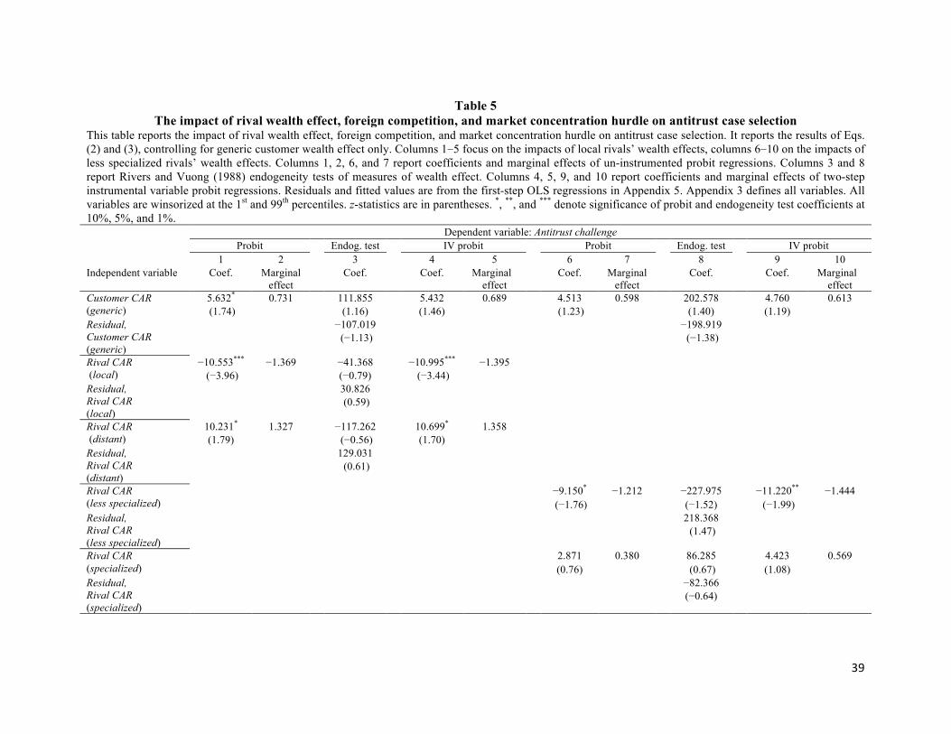
39

Table 5 The impact of rival wealth effect, foreign competition, and market concentration hurdle on antitrust case selection

This table reports the impact of rival wealth effect, foreign competition, and market concentration hurdle on antitrust case selection. It reports the results of Eqs. (2) and (3), controlling for generic customer wealth effect only. Columns 1−5 focus on the impacts of local rivals’ wealth effects, columns 6−10 on the impacts of less specialized rivals’ wealth effects. Columns 1, 2, 6, and 7 report coefficients and marginal effects of un-instrumented probit regressions. Columns 3 and 8 report Rivers and Vuong (1988) endogeneity tests of measures of wealth effect. Columns 4, 5, 9, and 10 report coefficients and marginal effects of two-step instrumental variable probit regressions. Residuals and fitted values are from the first-step OLS regressions in Appendix 5. Appendix 3 defines all variables. All variables are winsorized at the 1st and 99th percentiles. z-statistics are in parentheses. *, **, and *** denote significance of probit and endogeneity test coefficients at 10%, 5%, and 1%.

Dependent variable: Antitrust challenge Probit Endog. test IV probit Probit Endog. test IV probit 1 2 3 4 5 6 7 8 9 10

Independent variable Coef. Marginal effect

Coef. Coef. Marginal effect

Coef. Marginal effect

Coef. Coef. Marginal effect

Customer CAR (generic)

5.632* 0.731 111.855 5.432 0.689 4.513 0.598 202.578 4.760 0.613 (1.74) (1.16) (1.46) (1.23) (1.40) (1.19)

Residual, Customer CAR (generic)

−107.019 −198.919 (−1.13) (−1.38)

Rival CAR (local)

−10.553*** −1.369 −41.368 −10.995*** −1.395 (−3.96) (−0.79) (−3.44)

Residual, Rival CAR (local)

30.826 (0.59)

Rival CAR (distant)

10.231* 1.327 −117.262 10.699* 1.358 (1.79) (−0.56) (1.70)

Residual, Rival CAR (distant)

129.031 (0.61)

Rival CAR (less specialized)

−9.150* −1.212 −227.975 −11.220** −1.444 (−1.76) (−1.52) (−1.99)

Residual, Rival CAR (less specialized)

218.368 (1.47)

Rival CAR (specialized)

2.871 0.380 86.285 4.423 0.569 (0.76) (0.67) (1.08)

Residual, Rival CAR (specialized)

−82.366 (−0.64)

40

Table 5 (continued)

Dependent variable: Antitrust challenge Probit Endog. test IV probit Probit Endog. test IV probit 1 2 3 4 5 6 7 8 9 10Independent variable Coef. Marginal

effect Coef. Coef. Marginal

effect Coef. Marginal

effect Coef. Coef. Marginal

effectCombined CAR −1.640 −0.213 −20.014*** −1.043 −0.146 −23.143***

(−0.79) (−3.27) (−0.51) (−3.37) Residual, Combined CAR

18.897*** 22.751*** (2.63) (2.75)

Fitted value, Combined CAR

−17.390*** −2.207 −18.678*** −2.404 (−2.85) (−2.72)

Import ratio −4.564*** −0.592 −9.381*** −7.091*** −0.900 −4.245*** −0.562 −6.728** −7.068*** −0.910 (−4.76) (−4.58) (−5.78) (−3.90) (−2.19) (−4.82)

Census hurdle dummy 0.917** 0.170 1.941 0.993** 0.181 0.921** 0.175 1.933*** 1.026** 0.193(2.21) (1.37) (2.26) (2.40) (2.59) (2.43)

Industry growth −0.163 −0.021 0.054 −0.140 −0.018 −0.117 −0.015 0.273 −0.086 −0.011 (−0.79) (0.14) (−0.71) (−0.65) (0.96) (−0.54)

Relative deal size 0.581** 0.075 1.293*** 0.866*** 0.110 0.527** 0.070 1.252*** 0.837*** 0.108(2.48) (3.02) (2.89) (2.34) (3.39) (2.75)

Census bidder market share

−0.487 −0.063 −0.357 −0.317 −0.040 −0.431 −0.057 −1.162 −0.229 −0.029 (−1.43) (−0.61) (−0.80) (−1.32) (−1.39) (−0.59)

Ln Bidder market cap 0.281*** 0.036 0.165** 0.193*** 0.024 0.273*** 0.036 0.369 0.172*** 0.022(8.09) (2.50) (3.57) (7.49) (1.60) (3.19)

Year effects Y Y Y Y Y Y Pseudo R" 0.28 0.31 0.30 0.27 0.31 0.29 Observations 300 300 300 300 300 300

41

Table 6 The impact of local rival and distant rival wealth effects on antitrust case selection

(robustness test)The table reports robustness test results for the impacts of local rival and distant rival wealth effects on antitrust case selection. Panel A controls for local customer wealth effect, while panel B controls for reliant customer wealth effect. In panels A and B, columns 1 and 2 report coefficients and marginal effects of un-instrumented probit regressions. Columns 3 reports Rivers and Vuong (1988) endogeneity tests of measures of the wealth effect. Columns 4 and 5 report coefficients and marginal effects of two-step instrumental variable probit regressions. Residuals and fitted values are from the first-step OLS regressions in Appendix 5. Appendix 3 defines all variables. All variables are winsorized at the 1st and 99th percentiles. z-statistics are in parentheses. *, **, and *** denote significance of probit and endogeneity test coefficients at 10%, 5%, and 1%.

Panel A: The impact of local rival and distant rival’s wealth effects on antitrust case selection (controlling for local customer CAR) Dependent variable: Antitrust challenge Probit Endog. test IV probit 1 2 3 4 5 Independent variable Coef. Marginal

effect Coef. Coef. Marginal

effect Customer CAR (generic) 16.106** 2.046 −86.049 5.879 0.741 (2.39) (−0.56) (1.43) Residual, Customer CAR (generic) 103.415 (0.68) Customer CAR (local) −11.728*** −1.490 −330.889** (−2.80) (−2.11) Residual, Customer CAR (local) 319.796** (2.05) Fitted value, Customer CAR (local) −29.911 −3.768 (−1.21) Rival CAR (local) −8.349*** −1.061 53.955 −9.110** −1.148 (−2.55) (0.57) (−2.42) Residual, Rival CAR (local) −60.903 (−0.65) Rival CAR (distant) 6.944 0.882 1236.663* 5.282 0.665 (1.17) (1.81) (0.90) Residual, Rival CAR (distant) −1229.049* (−1.80) Combined CAR −1.967 −0.250 −25.299*** (−0.90) (−3.22) Residual, Combined CAR 22.950*** (2.65) Fitted value, Combined CAR −10.565* −1.331 (−1.65) Import ratio −4.752*** −0.604 2.428 −6.234*** −0.785 (−4.64) (0.40) (−4.99) Census hurdle dummy 0.894** 0.161 −6.745 0.830 0.145 (2.14) (−1.56) (1.56) Industry growth −0.197 −0.025 −2.171* −0.212 −0.027 (−0.89) (−1.76) (−1.01) Relative deal size 0.615*** 0.078 −2.353 0.728** 0.092 (2.64) (−1.39) (2.34) Census bidder market share −0.390 −0.050 −2.608** −2.253 −0.032 (−0.93) (−2.02) (−0.67) Ln Bidder market cap 0.263*** 0.033 0.554** 0.212*** 0.027 (6.55) (2.29) (4.72) Year effects Y Y Y Pseudo R" 0.30 0.35 0.30 Observations 282 282 282

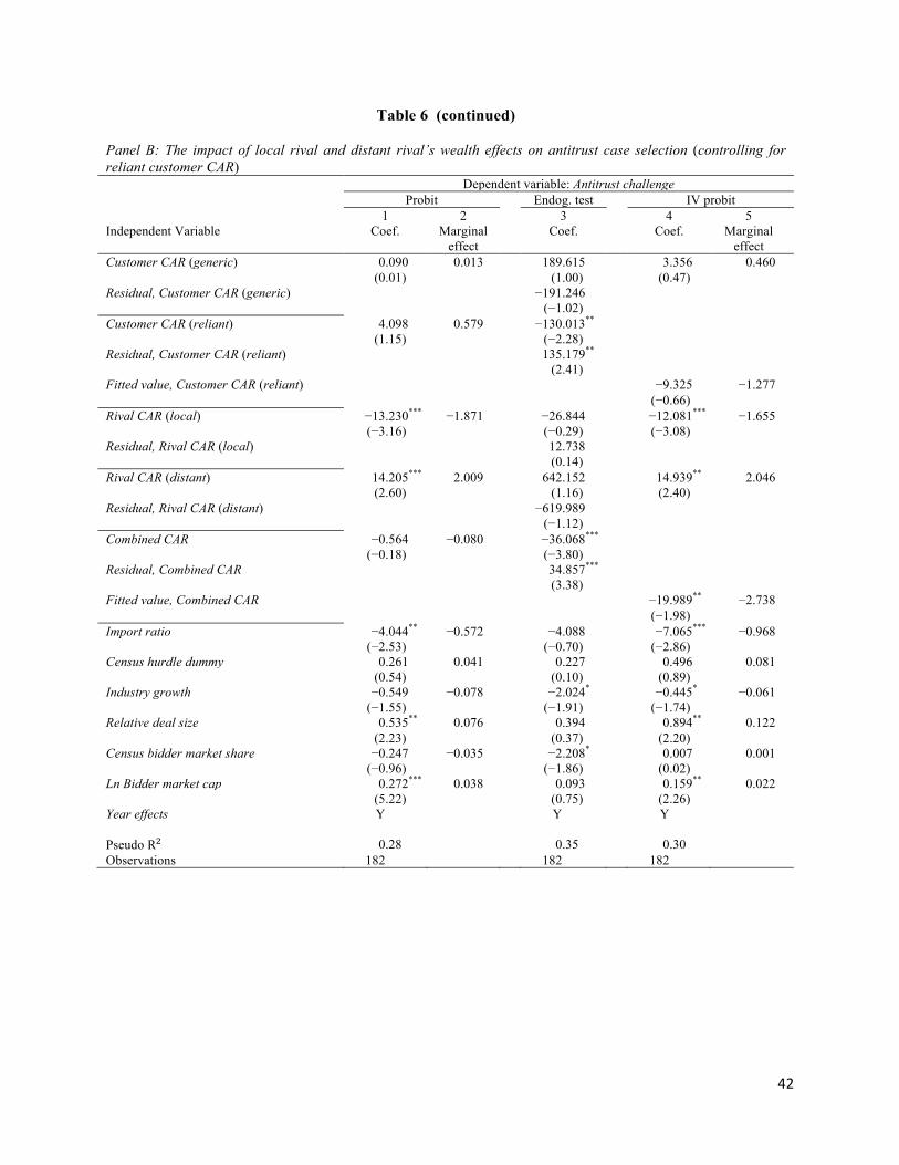
42

Table 6 (continued) Panel B: The impact of local rival and distant rival’s wealth effects on antitrust case selection (controlling for reliant customer CAR) Dependent variable: Antitrust challenge Probit Endog. test IV probit 1 2 3 4 5 Independent Variable Coef. Marginal

effect Coef. Coef. Marginal

effect Customer CAR (generic) 0.090 0.013 189.615 3.356 0.460 (0.01) (1.00) (0.47) Residual, Customer CAR (generic) −191.246 (−1.02) Customer CAR (reliant) 4.098 0.579 −130.013** (1.15) (−2.28) Residual, Customer CAR (reliant) 135.179** (2.41) Fitted value, Customer CAR (reliant) −9.325 −1.277 (−0.66) Rival CAR (local) −13.230*** −1.871 −26.844 −12.081*** −1.655 (−3.16) (−0.29) (−3.08) Residual, Rival CAR (local) 12.738 (0.14) Rival CAR (distant) 14.205*** 2.009 642.152 14.939** 2.046 (2.60) (1.16) (2.40) Residual, Rival CAR (distant) −619.989 (−1.12) Combined CAR −0.564 −0.080 −36.068*** (−0.18) (−3.80) Residual, Combined CAR 34.857*** (3.38) Fitted value, Combined CAR −19.989** −2.738 (−1.98) Import ratio −4.044** −0.572 −4.088 −7.065*** −0.968 (−2.53) (−0.70) (−2.86) Census hurdle dummy 0.261 0.041 0.227 0.496 0.081 (0.54) (0.10) (0.89) Industry growth −0.549 −0.078 −2.024* −0.445* −0.061 (−1.55) (−1.91) (−1.74) Relative deal size 0.535** 0.076 0.394 0.894** 0.122 (2.23) (0.37) (2.20) Census bidder market share −0.247 −0.035 −2.208* 0.007 0.001 (−0.96) (−1.86) (0.02) Ln Bidder market cap 0.272*** 0.038 0.093 0.159** 0.022 (5.22) (0.75) (2.26) Year effects Y Y Y Pseudo R" 0.28 0.35 0.30 Observations 182 182 182

43

Table 7 The impact of specialized rival and less specialized rival wealth effects on antitrust case selection

(robustness test) The table reports robustness test results for the impacts of less specialized rivals and specialized rivals wealth effects on antitrust case selection. Panel A controls for local customer wealth effect, while panel B controls for reliant customer wealth effect. In panels A and B, columns 1 and 2 report coefficients and marginal effects of un-instrumented probit regressions. Columns 3 reports Rivers and Vuong (1988) endogeneity tests of measures of the wealth effect. Columns 4 and 5 report coefficients and marginal effects of two-step instrumental variable probit regressions. Residuals and fitted values are from the first-step OLS regressions in Appendix 5. Appendix 3 defines all variables. All variables are winsorized at the 1st and 99th percentiles. z-statistics are in parentheses. *, **, and *** denote significance of probit and endogeneity test coefficients at 10%, 5%, and 1%.

Panel A: The impact of specialized rival and less specialized rival’s wealth effects on antitrust case selection (controlling for local customer CAR) Dependent variable: Antitrust challenge Probit Endog. test IV probit 1 2 3 4 5 Independent Variable Coef. Marginal

effect Coef. Coef. Marginal

effect Customer CAR (generic) 15.180** 2.046 −328.367 6.250 0.780 (2.13) (−1.15) (1.35) Residual, Customer CAR (generic) 346.025 (1.22) Customer CAR (local) −11.315** −1.490 −508.930** (−2.40) (−2.43) Residual, Customer CAR (local) 496.923** (2.37) Fitted value, Customer CAR (local) −24.705 −3.085 (−1.04) Rival CAR (less specialized) −10.384** −1.061 1311.240* −12.402*** −1.549 (−2.52) (1.86) (−2.91) Residual, Rival CAR (less specialized) −1320.172* (−1.88) Rival CAR (specialized) 5.536 0.882 307.022* 5.584 0.697 (1.63) (1.78) (1.54) Residual, Rival CAR (specialized) −301.351* (−1.75) Combined CAR −1.175 −0.250 −25.337*** (−0.52) (−3.16) Residual, Combined CAR 24.147*** (2.88) Fitted value, Combined CAR −11.733* −1.465 (−1.68) Import ratio −4.341*** −0.604 0.848 −6.151*** −0.768 (−4.01) (0.17) (−4.25) Census hurdle dummy 1.119*** 0.161 −4.182 1.180** 0.223 (3.06) (−1.42) (2.45) Industry growth −0.188 −0.025 −1.492* −0.199 −0.025 (−0.94) (−1.65) (−1.12) Relative deal size 0.548*** 0.078 −2.434 0.708** 0.088 (2.59) (−1.61) (2.46) Census bidder market share −0.375 −0.050 1.874 −0.244 −0.030 (−0.96) (1.19) (−0.68) Ln Bidder market cap 0.283*** 0.033 0.087 0.232*** 0.029 (6.91) (0.26) (4.41) Year effects Y Y Y Pseudo R" 0.32 0.38 0.33 Observations 290 290 290

44

Table 7 (continued) Panel B: The impact of specialized rival and less specialized rival’s wealth effects on antitrust case selection (controlling for reliant customer CAR) Dependent variable: Antitrust challenge Probit Endog. test IV probit 1 2 3 4 5 Independent Variable Coef. Marginal

effect Coef. Coef. Marginal

effect Customer CAR (generic) 3.119 0.447 232.229 1.918 0.266 (0.44) (1.00) (0.24) Residual, Customer CAR (generic) −231.164 (−1.01) Customer CAR (reliant) 0.617 0.088 −58.207 0.761 0.105 (0.20) (−1.01) (0.28) Residual, Customer CAR (reliant) 60.365 (1.04) Rival CAR (less specialized) −0.263 −0.038 −41.029 −0.398 −0.055 (−0.04) (−0.09) (−0.06) Residual, Rival CAR (less specialized) 43.079 (0.10) Rival CAR (specialized) −0.956 −0.137 60.679 0.116 0.016 (−0.24) (0.53) (0.03) Residual, Rival CAR (specialized) −61.048 (−0.55) Combined CAR −0.805 −0.115 −27.105*** (−0.32) (−3.64) Residual, Combined CAR 26.350*** (3.24) Fitted value, Combined CAR −21.593* −2.991 (−1.95) Import ratio −4.282*** −0.613 −7.981* −7.913*** −1.096 (−2.99) (−1.94) (−2.76) Census hurdle dummy 0.889** 0.177 2.774*** 0.978** 0.190 (2.38) (2.65) (2.38) Industry growth −0.288 −0.025 −0.395 −0.210 −0.029 (−1.17) (−0.50) (−1.30) Relative deal size 0.453*** 0.065 1.242* 0.800** 0.111 (2.60) (−1.72) (2.51) Census bidder market share −0.152 −0.022 −0.786 0.091 0.013 (−0.57) (−0.70) (0.28) Ln Bidder market cap 0.225*** 0.032 0.116 0.129 0.018 (3.88) (0.33) (1.62) Year effects Y Y Y Pseudo R" 0.27 0.33 0.30 Observations 197 197 197

45

Appendix 1: Summary of challenged deal details in the manufacturing sector Challenged cases in the study, listing bidder name, target name, their overlapping operating segment, the antitrust agency that files the challenge and the complaint issuance documented in the FTC and DOJ’s joint “Annual Report to Congress Pursuant to Subsection (j) of Section 7A of the Clayton Act Hart-Scott-Rodino Antitrust Improvements Act of 1976”. No. Announcement

Year Bidder Name Target Name SIC Fama-French

Industries Agency Record from Agency Report

1 1982 ConAgra Inc Peavey Co 2041 FOOD FTC FTC Consent agreement accepted July 19, 1982. Documented in 1982 annual report.

2 1982 Gulf Oil Corp Cities Service Co 2911 OIL FTC Civil Action No. 82-2131 (D.D.C. filed July 29, 1982).

3 1983 LTV Corp Republic Steel Corp(LTV Corp)

3312 STEEL DOJ Cv. No. 85-0884 (D.D.C. filed March 21, 1984).

4 1984 Texaco Inc Getty Oil Co 2911 OIL FTC FTC Consent agreement accepted July 10, 1984. Documented in 1984 annual report.

5 1994 IVAX Corp Zenith Laboratories Inc 2834 DRUGS FTC Docket No. C-3565, issued March 27, 1995.

6 1994 Boston Scientific Corp SciMed Life Systems Inc

3841 MEDEQ FTC Docket No. C-3573, issued April 28, 1995.

7 1995 Interstate Bakeries Corp Ralston-Continental Baking Company

2051 FOOD DOJ Cv. No. 95C4194 (N.D. Ill. filed July 20, 1995).

8 1995 Kimberly-Clark Corp Scott Paper Co 2621 PAPER FTC Cv. No. 3:95CV3055-P (N.D. Tex. Filed December 12, 1995).

9 1996 Lockheed Martin Corp Loral Corp 3812 CHIPS FTC Docket No. C-3685, issued September 19, 1996.

10 1997 Lockheed Martin Corp Northrop Grumman Corp

3812 CHIPS DOJ DOJ complaint issued March 23, 1998. Documented in 1998 annual report.

11 1998 Suiza Foods Corp Broughton Foods Co 2026 FOOD DOJ 99-CV-130, DOJ complaint issued March 18, 1999.

12 1998 Medtronic Inc Physio-Control International Corp

3845 MEDEQ FTC Docket No. C-3879, issued June 3, 1999.

13 1999 Rhone-Poulenc SA Hoechst AG 2834 DRUGS FTC Docket No. C-3919, issued January 28, 2000.

14 1999 Pfizer Inc Warner-Lambert Co 2834 DRUGS FTC Docket No. C-3957, issued July 28, 2000.

15 1999 Dow Chemical Co Union Carbide Corp 2869 CHEM FTC Docket No. C-3999, issued March 16, 2001.

16 1999 Rohm & Haas Co Morton International Inc

2899 CHEM FTC Docket No. C-3883, issued July 13, 1999.

17 1999 General Dynamics Corp Newport News Shipbuilding Inc

3731 SHIPS DOJ Civil No: 1:01CV02200, filed October 23, 2001.

18 1999 Litton Industries Inc Newport News Shipbuilding Inc

3731 SHIPS DOJ DOJ complaint issued July 9, 1999. Documented in 1999 annual report.

46

Appendix 1 (continued) No. Announcement

Year Bidder Name Target Name SIC Fama-French

Industries Agency Record from Agency Report

19 2000 Smithfield Foods Inc IBP Inc 2011 FOOD DOJ Civil Action No. 1:03CV00434 (HHK), filed 28 February, 2003.

20 2000 Valspar Corp Lilly Industries Inc 2851 CHEM FTC Docket No. C-3995, issued January 26, 2001.

21 2000 JDS Uniphase Corp E-Tek Dynamics Inc(Summit Partners LP)

3674 CHIPS DOJ C.V. No. C 00 2227 (THE) (N.D. Cal. Filed June 22, 2000).

22 2001 Valero Energy Corp Huntway Refining Co 2911 OIL FTC Docket No. C-4031, issued February 19, 2002.

23 2001 General Dynamics Corp Newport News Shipbuilding Inc

3731 SHIPS DOJ No. 1:01CV02200 (D.D.C. Oct.23, 2001).

24 2002 Pfizer Inc Pharmacia Corp 2834 DRUGS FTC Docket No. C- 4075, issued May 27, 2003.

25 2002 Northrop Grumman Corp

TRW Inc 3728 AERO DOJ No. 1:02CV02432 (D.D.C. filed Dec.11, 2002).

26 2003 Cephalon Inc CIMA Labs Inc 2834 DRUGS FTC Docket No. C-4121, issued September 20, 2004.

27 2004 Genzyme Corp ILEX Oncology Inc 2836 DRUGS FTC Docket No. C-4128, issued December 20, 2004.

28 2005 Teva Pharmaceutical Industries Ltd

IVAX Corp 2834 DRUGS FTC Docket No. C-4155, issued January 20, 2006.

29 2005 Procter & Gamble Co Gillette Co 2844 HSHLD FTC Docket No. C-4151, issued September 29, 2005.

30 2005 Boston Scientific Corp Guidant Corp 3841 MEDEQ FTC Docket No. C-4164, issued July 21, 2006.

31 2006 Watson Pharmaceuticals Inc

Andrx Corp 2834 DRUGS FTC Docket No. C-4172, issued October 31, 2006.

32 2007 CommScope Inc Andrew Corp 3357 STEEL DOJ No. 1:07-CV-02200 (D.D.C. filed Dec.6, 2007).

33 2009 Pfizer Inc Wyeth 2834 DRUGS FTC Docket No. C-4267, proposed order issued Oct.14, 2009.

34 2009 Merck & Co Inc Schering-Plough Corp 2834 DRUGS FTC Docket No. C-4268, proposed order issued Oct.29, 2009.

35 2009 Agrium Inc CF Industries Holdings Inc

2873 CHEM FTC Docket No. C-4277, proposed order issued Dec.23, 2009.

47

Appendix 2: Key variable construction process

1. Corporate customer identification

Following Shahrur (2005), we employ the Use table from the BEA Benchmark IO accounts to identify the

corporate customers of each horizontal merger. We include only single-segment customer firms to preserve test

power by excluding customers that have segments unrelated to the merging industry. This requirement excludes

customers firms that also have segments in the merging industry. Song and Walkling (2000) caution that merger

announcements release information about the merging industry and therefore affect firms that have segments in the

merging industry. The single-segment requirement pre-empts this confounding effect.

Similar to Shahrur (2005), we form generic, local, and reliant customer portfolios for our sample deals. We

construct a region-based local customer portfolio that includes all regional customers with an industry CIC over 1%.

For robustness, we replace region-based by a state-based geographic classification, i.e., defining a customer as local

if its headquarters is in either the target or bidder headquarter state, and find results that are qualitatively similar.20

The SDC, Compustat and the Use tables use different industry classifications, i.e., the SDC and Compustat use

four-digit SIC codes, while the Use table use six-digit IO codes. For IO–SIC matching, we adopt a series of

approaches. For the 1982, 1987, and 1992 Use tables, we follow Shahrur (2005) and use the conversion tables of

Fan and Lang (2000) to directly convert IO to SIC codes. We include an industry only if we can match its SIC code

to a unique IO code. For the 1997 and 2002 Use tables, since there is no direct IO–SIC mapping available, we adopt

the conversion strategy of Bhattacharyya and Nain (2011). First, we use the BEA IO–North American Industrial

Classification System (NAICS) conversion tables to convert IO codes to NAICS codes. 21 Then we use

correspondence tables from the U.S. Census Bureau to convert NAICS to SIC codes.22 Finally, we match all 1982,

1987, 1992, 1997, and 2002 Use tables data to our merger sample using SDC SIC codes.

Given that product market relations evolve over time, we use the 1982, 1987, 1992, 1997 and 2002 Use tables

for proposed deals during 1980–1986, 1987–1991, 1992–1996, 1997–2001, and 2002–2009 respectively. We find

similar results repeating our analysis using the 1982, 1987, 1992, 1997 and 2002 Use tables for deals occurring

during 1980–1984, 1985–1989, 1990–1994, 1995–1999, and 2000–2009 respectively. Our reported results use the

first matching set of Use tables since this involves minimum hindsight bias.

20The following states are in each of the regions. Northeast: Connecticut, Delaware, District of Colombia, Massachusetts, Maine, Maryland, New Hampshire, New Jersey, New York, Pennsylvania, Rhode Island, and Vermont. Southeast: Alabama, Florida, Georgia, Kentucky, Mississippi, North Carolina, South Carolina, Tennessee, and Virginia. Southwest: Arizona, Arkansas, Louisiana, New Mexico, Oklahoma, and Texas. Mideast: Illinois, Indiana, Michigan, Ohio, West Virginia, and Wisconsin. Midwest: Iowa, Kansas, Minnesota, Missouri, Nebraska, North Dakota, and South Dakota. West: Alaska, California, Colorado, Hawaii, Idaho, Montana, Nevada, Oregon, Utah, Washington, and Wyoming. 21The IO–NAICS concordance for 1997 is available in Appendix A of the “Benchmark Input-Output Accounts of the United States, 1997”, available at http://www.bea.gov/scb/pdf/2002/12December/1202I-OAccounts2.pdf. The IO–NAICS concordance for 2002 is available in Appendix A of the “U.S. Benchmark Input-Output Accounts, 2002”, available at http://www.bea.gov/scb/pdf/2007/10%20October/1007_benchmark_io.pdf. 22The 1997 and 2002 NAICS–SIC concordance tables are available at http://www.census.gov/eos/www/naics/concordances/concordances.html. In mapping IO to SIC for the 1997 and 2002 Use tables, for robustness, we further require that an IO code corresponds to a unique NAICS code and an NAICS code corresponds to a unique SIC code in order to retain a cleaner matching pattern, for the 1997 and 2002 Use tables. We find that this stricter restriction does not qualitatively change our conclusions. However, this restriction substantially reduces the number of identified 1997 and 2002 upstream–downstream industry pairs. Therefore, we do not apply this restriction.

48

2. Industry rival identification

Following Fee and Thomas (2004), we form generic, local, distant, less specialized, and specialized rival

portfolios for our sample deals. In particular, we construct a region-based local rival portfolio that includes all rivals

if their headquarters are in the same region as either the bidder’s or the target’s. For robustness, we also employ the

state-based classification and obtain similar results.23

Unlike customer portfolios, rival portfolios include single- and multi-segment firms. Although this adds noise

to the rival wealth effects, it preserves the influence construct because multi-segment firms are often large rivals

who play a significant influencing role. We exercise caution by excluding rivals who at the same time have

segments in the customer industry.

3. Measuring wealth effects at the merger announcement

To measure the wealth effects of related firms, we use an event study methodology and calculate abnormal

returns using the market model,

!"#$ = "#$ − () − *)"+$, where "+$ is the CRSP equally-weighted market index return on day t, "#$ is firm i’s return on day t and ()and *) are coefficients from the market model estimated over 250 trading days starting from day −300 before the

announcement date (day 0). We require a firm to have at least 100 daily returns available during the estimation

period. Our analysis uses the cumulative abnormal return from two days before to two days after the merger

announcement, i.e., CAR(−2, 2).

To calculate the combined wealth effect of merging firms (Combined CAR), we value-weight bidder and target

CAR(−2, 2) by the relative market capitalizations of the bidder and target at the fiscal year end before the merger,

excluding the value of any pre-merger holdings in the target by the bidder (e.g., Bradley, Desai, and Kim, 1988; Fee

and Thomas, 2004).

4. Import ratio as a measure of the level of foreign competition

Following Mitchell and Mulherin (1996) and Shahrur (2005), we measure the intensity of foreign competition

using the Import Ratio calculated as the merging industry’s total imports divided by its total domestic supply. Raw

data for constructing the Import Ratio are from the 1982, 1987, 1992, 1997, and 2002 BEA Use tables. Domestic

supply is commodity output minus imports, exports, change in private inventories and sales of scrap and used goods

(Streitwieser, 2010). We also follow Giroud and Mueller (2010) and Valva (2012) to use an alternative metric,

industry penetration (calculated as total value of imports divided by total value of imports plus domestic production)

and obtain similar results.

23There are 26 state-based local rivals (median of 9) and 80 distant rivals (median of 43) for an average deal. If we include only single-segment rivals, there are 12 state-based local rivals (median of 5) and 32 distant rivals (median of 20) for an average deal. This state-based local rival portfolio size is fairly close to Shahrur’s (2005) mean (median) state-based local rival portfolio size of 13 (4).

49

5. Market concentration

Sales-based HHI is a widely adopted measure of market concentration. To calculate it, previous literature uses

Compustat data or, more recently, U.S. Census Bureau census data (Bhattacharyya and Nain, 2011; Ahern, 2012).

Ali, Klasa, and Yeung (2009) find that HHI based on Compustat data has a correlation of only 13% with an HHI

based on census data. This is because Compustat covers only public firms whereas the U.S. Census Bureau census

covers public and private firms. We measure industry concentration using the Census Herfindahl Index for each

four-digit SIC industry, i.e., the census concentration estimate reported by the Census Bureau divided by 10000.24

We also calculate the change in concentration (i.e., ∆Census Herfindahl Index) as 2 × target market share × bidder

market share measured in the year before the merger announcement. Bidder and target market shares are Compustat

segment sales divided by census-based industry sales.

To test the market concentration hurdle hypothesis, we define a Census Hurdle Dummy according to the

criteria outlined in the 1992 DOJ/FTC Horizontal Merger Guidelines. In particular, Census Hurdle Dummy equals

one if a deal satisfies one of the following two thresholds: a) Census Herfindahl Index exceeds 0.18 and ΔCensus

Herfindahl Index is no less than 0.005, or b) Census Herfindahl Index is between 0.1 and 0.18 and ΔCensus

Herfindahl Index is no less than 0.01, otherwise zero.

In the 1982, 1987, and 1992 censuses, the U.S. Census Bureau conducted concentration data surveys only for

the manufacturing sector. From 1997 onwards, the census data cover the business service sector. For consistency,

we examine only manufacturing sector deals.

24Since the census is conducted every five years, it is impossible to derive an accurate concentration measure for each year. We use 1982, 1987, and 1992 SIC-based census concentration data and adjust 1997 and 2002 NAICS-based census concentration data for deals announced during 1980–1986, 1987–1991, 1992–1996, and 1997–2001, and 2002–2009 respectively. In the 1997 and 2002 censuses, U.S. Census Bureau data are provided on an NAICS basis. One SIC code may correspond to several NAICS codes and the matching relation changes over time. We therefore follow Ali, Klasa, and Yeung (2009) and adjust the data to form an SIC-based Census Herfindahl Index for 1997 and 2002. In particular, we take the sum of the sales-weighted HHI for each NAICS industry under one SIC. All census data are available at http://www.census.gov/econ/concentration.html.

50

Appendix 3: Variable definitions All variables are measured at the end of the fiscal year before the merger announcement, unless noted otherwise. Variable Definition Antitrust challenge Equals one if the DOJ or FTC challenges a merger according to the FTC

and DOJ’s joint “Annual Report to Congress Pursuant to Subsection (j) of Section 7A of the Clayton Act Hart-Scott-Rodino Antitrust Improvements Act of 1976”, zero otherwise. These reports are available on the FTC website, https://www.ftc.gov/policy/reports/policy-reports/ftc-annual-reports

Bidder past performance Bidder’s pre-acquisition return on assets, equal to the ratio of operating income before depreciation to total assets in the year before the merger announcement.

Census bidder market share Bidder sales in the merging industry divided by census-based total sales of the merging industry. Census data is available at http://www.census.gov/econ/concentration.html

Census Herfindahl Index The U.S. Census Bureau estimate of the industry Herfindahl index divided by 10000. Census data is available at http://www.census.gov/econ/concentration.html

∆Census Herfindahl Index Equals 2 × percentage of bidder sales in the merging industry × percentage of target sales in the merging industry. The merging industry’s total sales is estimated by the U.S. Census Bureau. Census data is available at http://www.census.gov/econ/concentration.html

Census hurdle dummy Equals one if a) the Census Herfindahl Index exceeds 0.18, and ∆Census Herfindahl Index is no less than 0.005, or b) the Census Herfindahl Index is between 0.1 and 0.18, and ∆Census Herfindahl Index is no less than 0.01, zero otherwise.

Combined CAR

A market-capitalization-weighted average of the bidder’s and target’s market-model-adjusted returns from two days before to two days after, i.e., (−2, 2), the announcement date.

Customer CAR (generic) Market-model-adjusted returns over a (−2, 2) window around the announcement date to an equal weighted portfolio of all corporate customers. A generic customer is a Compustat single-segment firm whose industry procures more than 1% of its input from the merger industry. The input-output relation is based on the 1982, 1987, 1992, 1997, and 2002 BEA Use tables, available at http://www.bea.gov/industry/io_benchmark.htm

Customer CAR (local) Market-model-adjusted returns over a (−2, 2) day window around the announcement date to an equal weighted portfolio of local corporate customers. A customer firm is local if it locates in the same region as the bidder or target.

Customer CAR (reliant) Market-model-adjusted returns over a (−2, 2) day window around the announcement date to an equal weighted portfolio of reliant corporate customers. A customer firm is reliant if it operates in a customer industry with the highest customer input coefficient (CIC) among all customer industries. CIC is the output value purchased from the merging industry divided by the customer industry’s total output value.

Customer dependence (generic) The generic customer’s reliance on the merging industry based on material purchases equals the weighted CICs of all customer industries, with weights being the ratio of each customer industry’s sales to the aggregate sales of all customer industries.

Customer dependence (local) The local customer’s reliance on the merging industry based on material purchases equals the weighted CICs of all local customer industries, with weights being the ratio of each local customer industry’s sales to the aggregate sales of all local customer industries.

51

Appendix 3 (continued) Variable Definition Customer dependence (reliant) The reliant customer’s reliance on the merging industry based on material

purchases is the CIC of the reliant customer industry. Customer relative size (generic) The ratio of the average generic customers’ market capitalization to the

bidder’s market capitalization, divided by 100. Customer relative size (local) The ratio of the average local customer’s market capitalization to the bidder

market capitalization, divided by 100. Customer relative size (reliant) The ratio of the average reliant customer’s market capitalization to the

bidder’s market capitalization, divided by 100. Customer relative size (local) The ratio of the average local customer’s market capitalization to the bidder

market capitalization, divided by 100. Customer relative size (reliant) The ratio of the average reliant customer’s market capitalization to the

bidder’s market capitalization, divided by 100. Delaware incorporation intensity (distant)

The proportion of Delaware incorporated rival firms in the merging industry of the distant rival portfolio, as a decimal.

Delaware incorporation intensity (generic)

The proportion of Delaware incorporated rival firms in the merging industry of the generic rival portfolio, as a decimal.

Delaware incorporation intensity (less specialized)

The proportion of Delaware incorporated rival firms in the merging industry of the less specialized rival portfolio, as a decimal.

Delaware incorporation intensity (local)

The proportion of Delaware incorporated rival firms in the merging industry of the distant rival portfolio, as a decimal.

Delaware incorporation intensity (specialized)

The proportion of Delaware incorporated rival firms in the merging industry of the specialized rival portfolio, as a decimal.

Hostile takeover dummy Equals one if a merger is hostile, zero otherwise. Import ratio The merging industry’s total imports divided by its total domestic supply.

Total domestic supply is commodity output minus imports, exports, change in private inventories and sales of scrap/used goods (Streitwieser, 2010). Raw data for import ratio construction is from the 1982, 1987, 1992, 1997 and 2002 BEA Use tables, available at http://www.bea.gov/industry/io_benchmark.htm

Industry-adjusted stock payment percentage

Equals the deal’s consideration paid in stock reported by the SDC (calculated as value paid in stock divided by total value) minus the average consideration paid in stock of all horizontal mergers in a merging industry in the year of merger announcement.

Industry growth The ratio of the median firm’s sales in an industry the year before the merger to industry median firm sales three years before.

Ln Bidder market cap. The logarithm of the bidder market capitalization in $millions. Relative deal size The ratio of deal value to the bidder’s market capitalization. Rival CAR (distant)

Market-model-adjusted return over a (−2, 2) window around the announcement date to an equal weighted portfolio of distant rivals. A rival firm is distant if it does not locate in the same region as the bidder or target.

Rival CAR (generic)

Market-model-adjusted return over a (−2, 2) window around the announcement date to an equal weighted portfolio of generic rivals. A generic rival is any Compustat firm operating in the merging industry the year before the deal announcement.

Rival CAR (less specialized)

Market-model-adjusted return over a (−2, 2) window around the announcement date to an equal weighted portfolio of less specialized rivals. A rival firm is less specialized if its R&D and advertising expenditure the fiscal year before the deal announcement is below the 75th percentile for the industry.

Rival CAR (local)

Market-model-adjusted return over a (−2, 2) window around the announcement date to an equal weighted portfolio of local rivals. A rival firm is local if it locates in the same region as the bidder or target.

52

Appendix 3 (continued) Variable Definition Rival CAR (specialized)

Market-model-adjusted return over a (−2, 2) window around the announcement date to an equal weighted portfolio of specialized rivals. A rival firm is specialized if its R&D and advertising expenditure the fiscal year before the deal announcement is above the 75th percentile for the industry.

Rival relative size (generic) The ratio of the average generic rival’s market capitalization to the bidder’s market capitalization.

Rival relative size (distant) The ratio of the average distant rival’s market capitalization to the bidder’s market capitalization.

Rival relative size (less specialized) The ratio of the average less specialized rival’s market capitalization to the bidder’s market capitalization.

Rival relative size (local) The ratio of the average local rival’s market capitalization to the bidder’s market capitalization.

Rival relative size (specialized) The ratio of the average specialized rival’s market capitalization to the bidder’s market capitalization.

Surprise deal dummy Equals one if there is no horizontal merger announcement in the merging industry in the three years before the merger announcement, zero otherwise.

Tender offer dummy Equals one if the transaction is conducted via a tender offer, zero otherwise.

53

Appendix 4: Instrument justification for wealth effect variables

1. Instrument justification for Combined CAR

For Combined CAR, we selected five instrumental variables, namely Surprise deal dummy, Tender offer

dummy, Hostile takeover dummy, Industry-adjusted stock payment percentage, and Bidder past performance.

Surprise deal dummy equals one if there are no horizontal mergers in the merging industry in the previous three

years. When a deal announcement surprises the market, the wealth effects are more pronounced. It is unlikely,

however, that the market can better predict anticompetitive mergers than efficient mergers or vice versa. We follow

the spirit of Aktas, de Bodt, and Roll (2004, 2007) and use Tender offer dummy, Industry-adjusted stock payment

percentage, and Bidder past performance as instruments. Tender offer dummy equals one if a deal is a tender offer

and zero otherwise. A tender offer often results in better acquirer wealth effects and long-run post-merger

performance (Agrawal and Jaffe, 2000) but as a mode of merger, a tender offer does not determine what drives a

merger and should have no link to antitrust intervention. Percentage of stock payment relates to bidder market

valuation (Travlos, 1987; Shleifer and Vishny, 2003; Rhodes-Kropf, Robinson, and Viswanathan, 2005), growth,

business complementarity, and information asymmetry (Hansen, 1987; Eckbo, Makaew, and Thorburn, 2014) and

therefore influences wealth effects. To ensure percentage of stock payment reflects information at the firm level, we

adjust it by the average percentage of stock payment of mergers in the same industry. This industry-adjusted

percentage of stock payment, as an arrangement of the medium of exchange, does not directly relate to

anticompetitive motives and thus is not directly related to antitrust intervention. Hostile takeover dummy equals one

if a merger is hostile and zero otherwise. Schwert (2000) finds deal hostility is associated with bidder wealth effects.

However, ex ante, deal hostility has no clear bearing on merger motives. Shivdasani (1993) and Schwert (2000)

suggest that hostile mergers improve efficiency by removing non-performing boards.

2. Instrument justification for rival CARs

For the CARs of rival portfolios, we use three instrumental variables, namely, Surprise deal dummy, Rival

relative size (following Aktas, de Bodt, and Roll, 2007), and Delaware incorporation intensity. Rival relative size

equals the ratio of a rival’s market capitalization to the bidder’s market capitalization (Appendix 3 gives a detailed

description). It relates to announcement effects because rivals that are similar in size are either more likely to face a

competitive disadvantage from a close competitor’s merger or are in a better position to capture potential efficiency

gains signaled by a horizontal merger. However, although these rivals may be more able to influence antitrust

intervention, their incentive to influence is conditional on their wealth effects. Therefore, Rival relative size affects

antitrust case selection only through rival wealth effects. Delaware incorporation intensity is the proportion of

industry rivals incorporated in Delaware. Delaware Antitakeover Law offers companies protection from unwanted

merger proposals, increases merger costs, and makes mergers more difficult to complete (Gaughan, 2015, p.106).

This attenuates rival wealth effects related to the merger. However, antitakeover legislation affects efficient and

anticompetitive mergers in a similar fashion and does not directly relate to antitrust intervention.

54

3. Instrument justification for customer CARs

For the CARs of customer portfolios, we instrument using Surprise deal dummy, Customer relative size, and

Customer dependence. Customer relative size is relative to bidder market capitalization. Larger customers may be

more likely to benefit from the efficiency gains of upstream mergers or sustain the impact of anticompetitive

upstream mergers. Customer dependence measures the customer’s reliance on the merging industry in terms of

material purchases. Reliant customers may have weaker bargaining power and be less likely to receive efficiency

gains from an upstream merger. They may be more vulnerable to an anticompetitive upstream merger due to greater

material purchase reliance along the supply chain. However, neither instrument relates to a particular type of

upstream merger motive.

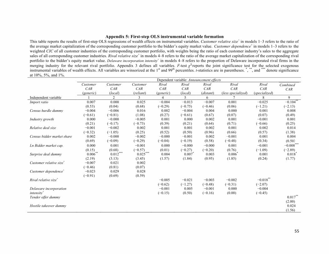
55

Appendix 5: First-step OLS instrumental variable formation This table reports the results of first-step OLS regressions of wealth effects on instrumental variables. Customer relative size+ in models 1–3 refers to the ratio of the average market capitalization of the corresponding customer portfolio to the bidder’s equity market value. Customer dependence+ in models 1–3 refers to the weighted CIC of all customer industries of the corresponding customer portfolio, with weights being the ratio of each customer industry’s sales to the aggregate sales of all corresponding customer industries. Rival relative size+ in models 4–8 refers to the ratio of the average market capitalization of the corresponding rival portfolio to the bidder’s equity market value. Delaware incorporation intensity+ in models 4–8 refers to the proportion of Delaware incorporated rival firms in the merging industry for the relevant rival portfolio. Appendix 3 defines all variables. F-test !"reports the joint significance test for the selected exogenous instrumental variables of wealth effects. All variables are winsorized at the 1st and 99th percentiles. t-statistics are in parentheses. *, **, and *** denote significance at 10%, 5%, and 1%. Dependent variable: Announcement effects Customer

CAR (generic)

Customer CAR

(local)

Customer CAR

(reliant)

Rival CAR

(generic)

Rival CAR

(local)

Rival CAR

(distant)

Rival CAR

(less specialized)

Rival CAR

(specialized)

Combined CAR

Independent variable 1 2 3 4 5 6 7 8 9 Import ratio 0.007 0.000 0.025 −0.004 −0.013 −0.007 0.001 −0.025 −0.104** (0.53) (0.04) (0.68) (−0.29) (−0.75) (−0.46) (0.06) (−1.21) (−2.13) Census hurdle dummy −0.004 −0.006 0.016 0.002 −0.004 0.004 0.000 0.001 0.008 (−0.61) (−0.81) (1.08) (0.27) (−0.61) (0.67) (0.07) (0.07) (0.49) Industry growth 0.000 −0.000 −0.005 0.001 0.000 0.002 0.001 −0.001 0.001 (0.21) (−0.17) (−0.73) (0.39) (0.21) (0.64) (0.71) (−0.66) (0.25) Relative deal size −0.001 −0.002 0.002 0.001 0.001 0.002 0.001 0.002 0.014 (−0.32) (−1.05) (0.25) (0.52) (0.50) (0.96) (0.66) (0.57) (1.38) Census bidder market share 0.002 −0.000 −0.002 −0.000 −0.001 0.002 −0.001 0.001 0.004 (0.69) (−0.09) (−0.29) (−0.04) (−0.19) (0.58) (−0.48) (0.34) (0.50� Ln Bidder market cap. 0.000 0.001 −0.001 0.000 −0.000 −0.000 0.001 −0.001 −0.008*** (0.15) (0.68) (−0.57) (0.01) (−0.27) (−0.20) (0.76) (−1.09) (−2.89) Surprise deal dummy 0.006** 0.012*** 0.025*** 0.004 0.007* 0.003 0.006* 0.001 0.018* (2.19) (3.13) (3.45) (1.57) (1.84) (0.95) (1.85) (0.24) (1.77) Customer relative size+ −0.007 0.021 0.002 (−0.46) (0.81) (0.07) Customer dependence+ −0.023 0.029 0.028 (−0.91) (0.69) (0.59) Rival relative size+ −0.005 −0.021 −0.003 −0.002 −0.018** (−0.62) (−1.27) (−0.48) (−0.31) (−2.07) Delaware incorporation intensity+

−0.001 0.005 −0.001 0.000 −0.004 (−0.15) (0.50) (−0.16) (0.00) (−0.45)

Tender offer dummy 0.017** (2.00) Hostile takeover dummy 0.024 (1.56)

56

Appendix 5 (continued) Dependent variable: Announcement effects

Customer CAR

(generic)

Customer CAR

(local)

Customer CAR

(reliant)

Rival CAR

(generic)

Rival CAR

(local)

Rival CAR

(distant)

Rival CAR

(less specialized)

Rival CAR

(specialized)

Combined CAR

Independent variable 1 2 3 4 5 6 7 8 9Industry-adjusted stock payment percentage

0.190 (0.91)

Bidder past performance 0.063 (1.28) Year effects Y Y Y Y Y Y Y Y Y #" 0.09 0.10 0.14 0.09 0.11 0.10 0.09 0.12 0.21 F-test!" 5.89 12.94*** 13.55*** 2.68 4.22 1.10 3.58 4.92 15.63*** Observations 372 354 266 372 363 371 371 372 372