BIS Papers No 8 1

What determines inflation in emerging market economies?

M S Mohanty and Marc Klau1

1. Introduction

Two major developments marked the monetary sector in emerging market economies (EMEs) in the 1990s. One was the steady decline in the inflation rate to low levels in the second half of the decade. The other was the growing preference for conducting monetary policy based on inflation targeting. For example, average inflation in 10 of the 14 EMEs discussed in this paper2 declined to a single digit rate in the second half of the 1990s, compared to only four in the first half. By the end of 2000, over half had switched to direct targeting of inflation. This change has meant a significant shift in the emphasis given to price stability in the monetary policy framework in EMEs as well as in the approach to controlling inflation. To be sure, this has underlined the key role for the central banks in the determination of inflation.

To understand the role of monetary policy in EMEs, it is crucially important to know the factors which determine inflation in these economies. Often two, rather different, claims are made regarding the inflation process in EMEs. First, inflation is hard to predict because it is affected by several non-monetary factors, most notably frequent supply shocks. These shocks tend to complicate the monetary transmission mechanism by blurring the role of demand side factors in the inflation process. In addition, as these factors are not easy to control and not enough information is available, it is often difficult for the central bank to be sure about their exact impact on the general price level and to take account of them in formulating monetary policy. The other view is that non-monetary factors influence only the short-run path of inflation. In the long run, monetary variables determine the inflation rate. Therefore, it is argued, the standard output gap models should provide a reasonable explanation of the inflation dynamics in EMEs. This also explains why central banks should worry about the current and future path of aggregate demand in the economy.

The reality for EMEs may, however, lie somewhere between the two paradigms. Empirical studies have not resolved the debate surrounding the causes of inflation in developing economies, particularly when it is low. Research has, nevertheless, found that high inflation tends to be associated with monetisation of excessive fiscal deficits, aggravated by a high degree of indexation of wages and prices and frequent devaluation of the exchange rate. But with the inflation rate declining in recent years, a fresh look at the inflation process in EMEs is necessary to throw light on at least two important issues. First, what are the major factors behind the inflation process in EMEs? Second, what implications do these factors have for the conduct of monetary policy? The objective of this paper is to address these issues by analysing a quarterly model of inflation using more recent information. The paper follows an eclectic approach, where both demand and supply factors are seen to drive prices. However, the paper is not intended to be exhaustive in its examination of the factors that cause inflation in EMEs. In fact, depending on the country characteristics, there may be several other influences, which are either difficult to quantify or for which no satisfactory data are available.

The empirical results reveal that the conventional determinants of inflation, such as the output gap, excess money supply and wages, have a significant influence on inflation. However, their unique importance could not be established for all countries. Supply factors affect inflation in a large number

1 We are grateful to Palle S Andersen for his extremely valuable suggestions and comments at each stage of preparing this

paper and to Stefan Gerlach for many useful and stimulating discussions on the inflation processes in EMEs. The errors that remain are solely ours. The views expressed in the paper are also our own and do not represent those of the Bank for International Settlements.

2 Brazil, Chile, the Czech Republic, Hungary, India, Korea, Malaysia, Mexico, Peru, the Philippines, Poland, South Africa, Taiwan (China) and Thailand.

2 BIS Papers No 8

of countries. Shocks to food prices emerge as the most common inflation determinant in almost all EMEs, followed by the exchange rate. In contrast, inflation and oil price shocks are only weakly associated. In some countries, monetary policy did not accommodate these shocks. Different degrees of adjustment of domestic oil prices to changes in international prices may have played an additional role in this outcome. An important implication of these findings is that to the extent that agricultural shocks and large unexpected movements in the exchange rate affect inflation and diminish the importance of demand management policy, they complicate the conduct of monetary policy and introduce considerable uncertainty regarding its impact on prices. The role of monetary policy is more transparent and its impact more effective when inflation is primarily driven by demand shocks and when demand changes can be accurately captured by indicators such as the output gap or monetary growth. In contrast, a significant influence of supply factors on prices raises issues about the appropriate target for policy. The dominance of agricultural shocks and exchange rate movements in the inflation process also highlights the need to liberalise agricultural trade to reduce the volatility of food prices, and to stabilise the exchange rate to promote price stability in EMEs.

The remainder of the paper is divided into four sections. Section 2 reviews price developments in 14 selected EMEs and discusses the main determinants of inflation. Section 3 develops the theoretical model, while Section 4 presents the empirical results. Policy implications are discussed in Section 5.

2. A review of trends and determinants of inflation in EMEs

Trends in the 1990s Many EMEs have had a history of moderate to high inflation, typically associated with either expansionary fiscal and monetary policies and/or large depreciation of exchange rates.3 Inflation rates in EMEs have been highly sensitive to various internal and external price shocks, particularly those arising from large changes in import and food prices. However, conditions changed over the 1990s and most EMEs managed to reduce their inflation rates considerably during the second half of the decade.

Table A1 in the annex shows the mean and standard deviation of the annual headline inflation rate in 14 EMEs during the 1970s, 1980s, and the first and second halves of the 1990s. What is evident from Table A1 is that inflation declined during the 1990s, the rate of decline being fastest during the second half. In the Asian economies, average inflation fell from a range of 5�15% in the 1970s to 2�8% in the second half of the 1990s, with most countries witnessing a gradual but slow rate of disinflation over this period. In Korea, mean inflation declined from 15% in the 1970s to only 4½% by the second half of the 1990s. This trend is broadly shared by Malaysia, Taiwan (China) and Thailand, where average inflation has not only stayed within a single digit range during the past three decades but to between 2 and 5% by the second half of 1990s. Compared to their Asian neighbours, India and the Philippines have experienced relatively higher inflation, which exceeded 8% and 10%, respectively, up to the mid-1990s, but then fell to below 8% in the latter half of that decade. The Asian crisis did not seem to pose a lasting problem on the inflation front. In the crisis-hit economies (Korea, Thailand, Malaysia and the Philippines), inflation did rise to high levels in 1998 but fell sharply in 1999 following the implementation of stabilisation programmes.4

Latin American countries have witnessed a much faster rate of disinflation. In Chile, average inflation declined from over 140% in the 1970s to about 6% during the second half of the 1990s. Chile�s anti-inflation strategy has been helped by the implementation of a comprehensive structural reform programme to boost productivity, a conservative fiscal policy, a crawling exchange rate peg and an independent monetary policy. In Peru, inflation averaged 25% in the 1970s but then rose above 300%

3 Following Dornbusch and Fischer (1993), we define a moderate and high rate of inflation as 15-30% and 30-100% annually,

respectively, over at least three years. 4 In Indonesia, however, inflation declined only temporarily after the crisis. The recent burst of inflation there has been fuelled

by rapid currency depreciation and rising fiscal deficits.

BIS Papers No 8 3

by the first half of the 1990s. However, helped by a stabilisation programme focused on reducing the fiscal deficit to a low level, abolishing wage indexation in the public sector and allowing the exchange rate to be market determined, Peru succeeded in reducing inflation to less than 4% in 1999.

Following several large devaluations of the currency and very high rates of growth of the money supply, Brazil recorded exceedingly high levels of inflation throughout the first half of the 1990s, even compared to the 1970s and the 1980s. However, a dramatic turnaround began in the second half of the 1990s and since 1997 the inflation rate has been in a range of 4�6%. This period coincided with the introduction of the Real Plan, implementation of major fiscal reform programmes and a tightening of monetary policy. The period also witnessed a significant overvaluation of the exchange rate, culminating in a large devaluation in early 1999. However, unlike previous episodes, the devaluation had only a moderate impact on the rate of inflation. In Mexico, inflation fell steadily to a single digit rate in 1993 and 1994. Following the crisis and a sharp devaluation of the currency, inflation rose again to over 30% in 1995 and 1996. However, helped by a stabilisation programme centred on reducing the fiscal deficit, stopping high wage inflation and allowing the exchange rate to move freely, Mexico succeeded in reducing inflation to a single digit rate by 2000.

A common aspect of the inflation process in the central European economies during the 1990s was the large-scale deregulation of prices following the transition to market economy. The average rate of inflation in Hungary rose from about 14% in the 1980s to over 25% in the first half of the 1990s, a period beset with two large devaluations, growing fiscal problems and large relative price shifts. Following a comprehensive fiscal stabilisation programme accompanied by monetary tightening and a switch to a preannounced crawling peg system in 1995, the inflation rate declined in the second half of the 1990s. In the Czech Republic, following a large devaluation and liberalisation of prices at the beginning of the 1990s, prices grew relatively fast during the first half of the decade. Between 1993 and 1997 the exchange rate peg played an important role in containing inflationary pressures. But in the face of large capital inflows and increases in wages far in excess of productivity growth, the currency came under pressure, resulting in a steep devaluation in May 1997 and subsequent abandonment of the exchange rate peg. The inflation rate rose to over 10% in 1998, but then fell to about 2% in 1999.

Poland experienced hyperinflation in the early part of the 1990s. Following a broad-based stabilisation programme including an exchange rate peg, Poland succeeded in arresting the rapid growth in prices. However, inflation stabilised within the range of 30�60%, reflecting pressures stemming from a crawling peg, backward-looking indexing of wages, high fiscal deficits, capital inflows and liberalisation of regulated prices. The subsequent stabilisation efforts, however, reduced the inflation rate to a single digit level by 1999.

South Africa experienced double digit inflation in the 1980s and the first half of the 1990s, reflecting high fiscal deficits, growing nominal rigidities in factor and product markets and a steady depreciation of the exchange rate. In 1993, inflation started to decline following the implementation of deeper structural reforms. Much of the improvement was concentrated in the years 1998 and 1999, when a greater degree of fiscal and monetary discipline was enforced.

Two distinct aspects of inflation in EMEs are clearly evident from the above discussion. First, different regions have witnessed different speeds of disinflation. In the Asian economies, inflation has fallen rather gradually over a long period and the volatility of inflation has been low. In the Latin American and central European economies, on the other hand, the recent decline in inflation has followed a period of rapid increase in prices. These countries have undergone a much sharper rate of disinflation and the volatility of inflation has remained high. Given the different experiences, an important question is how the inflation history affects the degree of inflation persistence. A second question is the extent to which any one or more factors were responsible for sustained increases or decreases in inflation. Fiscal policy in particular played a key role in the inflation process in many countries, while the influence of the exchange rate regime is more difficult to assess. A number of countries relied on a fixed exchange rate regime as their nominal anchor, but ultimately were unsuccessful in defending the peg. In others, disinflation has coincided with the introduction of a more flexible regime. One important aspect, which is not so clearly evident from the discussion so far, is the role that supply factors played in aggravating or dissipating price pressures in different countries. In what follows, a brief review of inflation determinants is presented to identify the transmission mechanism in the 14 economies.

4 BIS Papers No 8

Determinants of inflation An important reason for sustained rates of high inflation in the EMEs is the vicious nexus between fiscal deficits, monetary growth and inflation (Montiel (1989), Dornbusch (1992) and Bruno (1993)). According to Burton and Fischer (1998), the average seigniorage revenue in the moderate-inflation economies was about 1.8% of GDP before stabilisation but declined to about 1.5% after inflation was reduced. This seigniorage revenue was associated with average fiscal deficit/GDP ratios and narrow money (M1) growth rates of 4% and 24%, respectively, before stabilisation and 0.3% and 12% after stabilisation.

However, differences in inflation performance cannot be attributed to differences in fiscal performance alone. The adaptability of fiscal systems to external shocks has been a contributing factor. For example, a low fiscal deficit and a relatively equal distribution of income (which facilitates sharper adjustment of fiscal deficits) in the East Asian economies are cited as important factors in their better inflation performance than the Latin American economies, which lack these conditions (IMF (1996)). A sound fiscal balance, though necessary, is not, however, a sufficient condition to rein in inflation if monetary policy remains loose and accommodates the private sector�s excess demand for credit, as was the case in many East Asian countries before the 1997-98 crisis. Whatever the cause, excess demand arises if monetary growth remains higher than needed to support growth. A straightforward implication of this is that inflation will rise until real demand falls to the level consistent with potential output. Conversely, a sustained decline in inflation can be identified with a long-term improvement in the fiscal position and a lower rate of monetary growth that push actual output closer to potential. Changes in the output gap should, therefore, explain most of the policy-driven changes in inflation.

In contrast to the �fiscal� view of inflation, the �balance of payment� view emphasises the role of the exchange rate in the determination of domestic prices.5 Conventional wisdom holds that countries that are prone to large external shocks should allow their exchange rate to move to correct the external disequilibrium. An important consequence of opting for a flexible exchange rate is that domestic prices are partly determined by the exchange rate. As a first-round effect, movements in the exchange rate directly affect inflation by changing the domestic currency price of imports. The second-round effect depends on how this initial shock is transmitted into other sectors through changes in costs and inflation expectations. Where maintaining domestic price stability takes precedence over external stability and the authorities opt for a fixed exchange rate regime, the exchange rate, of course, has no impact on inflation. In fact, the burden of adjustment to external shocks falls on fiscal policy.

Empirical evidence is, however, ambiguous on whether a fixed or a flexible exchange rate leads to lower inflation. Some cross-sectional studies show that inflation is lower under pegged exchange rate regimes than under flexible regimes (Edwards (1993) and Ghosh et al (1995)). But this result is typically true of fixed regimes that were not subjected to frequent adjustments. Others have attributed this result to lower rates of monetary growth in the fixed exchange regimes or what is called a �monetary disciplining effect� of the regime, and to the fact that a part of excess money growth may appear as a balance of payments deficit in the absence of an offsetting change in the exchange rate (Fielding and Bleaney (2000)). The latter effect is, however, only temporary since the external deficit will eventually require a correction. Ultimately, the inflationary impacts of a fixed exchange rate regime depend on the credibility of the regime, particularly in the context of an open capital account and financial imperfections such as a weak banking system (Kaminsky and Reinhart (1999)). Others argue that the inflationary consequences of the exchange rate depend on the nature of external shocks � temporary or permanent � and whether or not a real depreciation is warranted (Chang and Velasco (2000)). As Siklos (1996) concludes, countries with fixed regimes often experience higher, rather than lower, average inflation because the regimes are not credible. On the other hand, Quirk (1994) argues that differences attributed to the various exchange rate regimes tend to narrow once adjustments are made for the influence of other factors. The country experiences, nevertheless, show that, irrespective of regime, the exchange rate is an important determinant of inflation in a number of EMEs (Kamin and Klau (2001)).

A third important factor is the rate of wage inflation. The role of wages in inflation dynamics in EMEs has received attention from two major angles. One is that an exogenous wage shock can lead to cost-push inflation if the monetary authorities follow an accommodative policy. The other is that the

5 See Montiel (1989) for a discussion on the two schools of thought.

BIS Papers No 8 5

backward-looking indexing mechanism, by which current wages follow past inflation, can give rise to strong persistence effects. Dornbusch and Fischer (1993) note two specific features of the indexation mechanism in the high- to moderate-inflation economies that could produce such effects. First, indexation encourages longer-term contracts, which make the inertia effect particularly strong. Second, the typical indexing formula tends to make real wages a negative function of inflation, implying that real wages and unemployment increase when the inflation rate is reduced. The resulting output cost may discourage authorities from engaging in a process of sustained disinflation. In addition, the wage indexation mechanism may play a role in the transmission of exchange rate movements to inflation, since the frequency with which wages are revised tends to increase when the inflationary pressures are driven by exchange rate depreciation (Leviathan and Piterman (1986)). This has been an important factor in the inflation episodes of some of the Latin American and transition economies, where devaluation-induced inflation has had higher persistence effects than inflation driven by domestic factors. Empirical studies have also confirmed the significant role of wages in the inflation dynamics in a number of EMEs (Montiel (1989) and Agénor and Hoffmaister (1997)).

A particularly important factor in the EMEs context is the role that relative prices play in the inflation process. In classical models of inflation, relative price changes do not affect aggregate inflation, since industry level price variations are expected to be mutually offsetting in nature; only aggregate demand changes have implications for the rate of inflation. However, the role of relative prices in inflation has received increasing attention since Ball and Mankiw (1994 and 1995) demonstrated that firms react differently to a large price shock than to a small price shock. Since firms face costs in adjusting prices they would react to a large shock by revising prices but ignore small shocks. Hence the impact of a relative price shock on inflation depends on its distribution: the more it is skewed to either side the greater the impact on the overall inflation. Apart from this, two factors may explain why relative prices play a relatively larger role in the inflation process in the EMEs.

First, certain relative price changes, particularly those arising from large supply shocks may have major macroeconomic implications (Fischer (1981)). The size of the overall price impact, even if the shock is only temporary, depends on how important the sector in question is for overall consumer inflation. For example, food and energy account for a relatively larger share of the consumer price index in the EMEs than in the industrialised economies. A sharp rise in prices of these commodities not only raise short run inflation, by virtue of their high weight in the consumer price index, but also can lead to a sustained rise in the inflation rate if it raises inflation expectations.6 Second, to the extent that supply shocks are accommodated by monetary policy they give rise to demand-driven inflationary pressures.

An important source of relative price volatility in EMEs is administered prices. Despite their diminishing importance, revision or liberalisation of administered prices has had inflationary outcomes, in particular in transition economies. Whether or not administered prices can be a major source of inflation depends on the nature of price adjustments and the extent to which monetary policy remains neutral. If administered prices are revised periodically to restore their relative level, they may not affect average inflation (Phillips (1994)). Nonetheless, adjustment of administered prices can be inflationary. First, they may be accommodated by monetary policy. Second, as the experience of the transition economies has shown, price increases in administered sectors were not fully compensated by price decreases in the non-administered sectors. Hence, average prices rose in these economies (IMF (1996)). Moreover, price liberalisation has in many cases been spread over a long period of time, leading to continuing adjustment of relative prices and increases in inflation. Recent research has confirmed that relative prices did have a significant impact on inflation in the transition economies and that this impact was not necessarily temporary (Coorey et al (1998), Pujal and Griffiths (1998)).

Another factor is the extent to which inflation persists on its own through various mechanisms which link current inflation to past inflation. Inflation persistence stems from both backward-looking inflation expectations and indexation of wages and prices to past inflation. Thus, stopping high inflation has typically involved efforts to break the mechanisms that give inflation its own momentum (Sargent (1982)). While a low degree of persistence is highly desirable for the success of the disinflation process, it is not entirely clear if that would be the case once inflation has been stabilised at a low

6 The inflation volatility arising from fluctuations in food prices may have a higher persistence effect if supply adjustments are

constrained by domestic and international trade restrictions.

6 BIS Papers No 8

level. To the extent that low inflation and credible monetary and fiscal policies anchor inflation expectations better, they might lead to more persistent inflation, thus helping the central banks in their efforts to maintain price stability. In such an environment, a temporary shock has very little initial impact on the prospects of price stability. But the challenges for the central banks are considerable when low policy credibility leads to a high degree of persistence of inflation and high costs of disinflation.7

How far do the above factors explain the actual movement of inflation in various countries? Tables A2 to A8 present data on average values of potential determinants of inflation during the 1980s and the first half of the 1990s and annual trends during the second half of the 1990s. These indicators include annual percentage changes in broad money, output gaps and unemployment rates, as demand side factors, and growth rates of nominal wages, exchange rates, import prices and prices of food and oil components in the CPI index, as cost or supply side factors. There are, however, some important gaps in the data. Data on unemployment, wages and food and oil prices are not available for the entire sample period for all the EMEs. In particular, some data series for the transition economies only start in 1990. Second, as data on administered prices are not easily available, we exclude them from further analysis although they are an important determinant of inflation in many EMEs. The following trends are easily discernible from the tables:

� None of the indicators used to track the demand side picture of inflation appear to have moved closely with inflation (see Tables A2 to A4). Output gaps seem to be poorly related to inflation, particularly during the second half of the 1990s:8 both variables moved in opposite directions in the first three years but in the same direction in the last two years. The correlation coefficient between these two variables during the 1990s was negative for only six countries and positive end reasonably high for only four (Table A9). The weak association is also evident from Graph 1;

� The growth of broad money is typically high in high-inflation economies. Nevertheless, except for Brazil and Peru, which experienced a contraction in money supply growth during the second half of the 1990s, it is not apparent that the recent decline in inflation has been associated with a significant reduction in monetary growth. In fact, the correlation coefficient between these two variables is negative for roughly half the countries in our sample;

� The correlation coefficient between the unemployment rate and inflation is negative in only five countries. However, there are signs of a closer relationship in the more recent period when, in several countries, higher unemployment coincided with declining inflation;

� Exchange rate changes and inflation appear to be closely linked. This is true for all regions although the degree of pass-through seems to be higher for the Latin American countries, where rapid disinflation has usually been accompanied by significant nominal appreciation of currencies. The correlation coefficient between inflation and changes in the exchange rate is positive in all but four countries, with particularly high values for Brazil, Hungary, Korea and Mexico;

� Wage inflation has been high in Latin American and transition economies as well as in South Africa. Typically, nominal wage growth has exceeded inflation during the 1990s. The notable exceptions are Hungary, the Philippines and Peru, where real wage growth has been negative. The correlation coefficient between nominal wage growth and inflation is positive and strong in the Latin American countries, but less so in other countries and actually negative in some cases;

� A large part of the movement in inflation seems to come from the two major components of the price index, food and oil prices. The changes in these two indices are, however, highly

7 Blanchard (1998) points out three essential features of successful disinflation: (i) the credibility of the monetary authority

implying coherent fiscal and monetary policy, (ii) a wage setting process that is less tilted to nominal overhang and (iii) a flexible labour market enabling the authorities to enforce a real wage cut.

8 The estimates of the output gap are based on quarterly GDP data and are measured as the proportionate deviation of actual output from potential, with the latter calculated by applying the HP smoothing procedure to separate the trend and cyclical components of GDP. We also use alternative estimates of potential output to test the empirical relevance of this variable in forecasting inflation.

BIS Papers No 8 7

irregular, suggesting that they are largely determined by supply conditions (Table A7). The extent of supply side influences on inflation is evident from the high correlation between overall inflation and food price inflation. It needs, however, to be noted that since food prices constitute a large part of the consumer price index in all EMEs, a high degree of comovement of these two variables is to be expected. But to the extent that food prices are determined by exogenous factors, this provides a rough idea about the supply side influence on inflation in these economies. Surprisingly, oil prices seem to be a less important factor; in fact, the correlation is negative in six out of the 14 countries;

� The role of import prices in the recent disinflation episode is evident in many EMEs as import prices, including oil, have increased at a significantly lower rate than overall inflation (Table A8). Given the high correlation between import prices and the exchange rate, it is not clear which factor is the more important determinant of inflation, though the bilateral correlation coefficient in Table 9 points to the latter.

3. The model and the data

In this section, we turn to empirical estimates of inflation, using a common specification that accounts for both demand and supply side factors as discussed above. Following Gordon (1985), a general specification for inflation can be obtained by combining a wage equation with a markup price equation, along the lines of the standard augmented Phillips curve. The equation for unit labour costs can be expressed as a function of current and lagged inflation, the output gap,9 the difference between actual and trend productivity growth and various supply shift factors:

� � � � � �� � � �� �������������j

wt

witjt

Attttt zLLLpLw ����� 4

*321

* � (1)

where w and p are natural logs of wages and prices, respectively, A� and *

� are growth rates of

actual and trend productivity, �� is the output gap measured as the proportionate deviation of actual from potential output, z is a vector of variables representing supply shift factors and (L) is the lag operator.

A markup equation for the changes in prices can be expressed in a similar fashion:

� �� � � � � �� � pt

piti i

*t

Att

*ttt (L)zβLβLβwLβp �������������� � 4321

� (2)

For simplicity the two supply shift factors for the labour and product markets are combined into one �z� vector. Moreover, assuming that wages do not depend on the current period inflation, the reduced form inflation equation, after denoting the complex set of lagged coefficients by )()()( LLL iii ��� � and adding a constant, can be written as:

� � � � � � � � � � pt

wtiti it

Atttt LLLLpLp �������� ������������� �� 14

*32110 z)(� (3)

In order to make the model operational for the EMEs, we make a few changes to the basic specification. First, since it is not easy to obtain reasonable and reliable estimates of productivity growth, we exclude this term from the empirical version of the equation.10 Second, although equation (3) rules out a direct role of wages by assuming the same set of determinants for unit labour cost as for the markup price specification, we introduced nominal wages into the model where data were available. This was based on the consideration that indexation plays an important role in the inflation process in many EMEs.

9 Because data on unemployment rate are not available for all countries, we have used the output gap as a proxy for labour

market conditions. 10 Evidence suggests that the rise in total factor productivity has played a role in the growth experience of several EMEs, and

has worked its way through to the final consumer by way of lower product prices. However, data for long time spans are not yet available to enable empirical testing of this hypothesis.

8 BIS Papers No 8

Third, in most inflation models for industrialised countries, demand indicators are represented by one single variable (the output gap) while monetary variables do not directly enter into the model. The underlying rationale is that the transmission of monetary policy takes place through changes in aggregate demand and there exists a strong link between the interest rate and demand in these economies. This relationship is quite central to the monetary transmission mechanism and looks plausible for developing economies as well. There are, however, important differences between the two cases. One is that estimates of the output gap for developing economies are not very precise and, therefore, may not fully capture the demand dynamics. In such a case, some measure of excess money growth along with the output gap could help measure demand developments better. Another is that, given the relatively underdeveloped state of financial markets and the weak relationship between the interest rate and inflation, money supply growth could be an important indicator of future demand growth and hence inflation expectations.

Two different approaches are available for directly including monetary variables in addition to the output gap. One is proposed by Gordon (1985), and links current period output growth to excess money growth and actual velocity growth by the following two identities:

ttt py ��������

���1 and ttt vmy ����� �

where ∆ŷ and ∆m and ∆v are the growth rates of nominal GDP in excess of the growth of potential GDP, excess money growth and actual velocity growth, respectively. Making use of these two identities and assuming further that inflation depends not only on the current period output gap but also on the change in the gap, the inflation model in equation (3) can be written in terms of both the output gap and monetary variables (see Gordon (1985) for details of the derivation). The other approach is to let the money gap appear as an additional variable on the strength of its being an indicator of inflation expectations (Coe and McDermott (1997)). We follow the second approach and specify the money gap in two different ways for two different groups of countries. For countries where the money demand function appears to be stable, we use a partial adjustment framework specified as:

ds� ttt mmm �� and d13210

dt-ttt miym ���� ����

where md and ms are the natural log of demand for and supply of broad money, respectively, y is the log of real GDP and i is the nominal short-term interest rate. For countries for which we did not get a stable money demand function or which have long ago moved away from monetary targeting, we constructed a real money gap variable, measured as the proportionate deviation of the actual real money supply from its trend value, obtained through a simple time trend equation:

TR� ttt mmm ��

We chose four supply side variables: the rate of change in the exchange rate (∆et), and shocks to import prices (∆mpt � ∆pt-1), food prices (∆fpt � ∆pt-1), and oil prices (∆opt � ∆pt-1). As is evident from the notation, a price shock is defined as the deviation of percentage changes in that variable from the previous period inflation rate. In defining the shocks in this way, the model overcomes the potential problems of regressing the inflation rate on its components. Since changes in the exchange rate and import prices are closely related, we use them alternately. The final version of the model for estimation is thus:

� � � � � � � � � � � �

� � � � ttttt

tttttttt

popLpfpL

pmpLwLeLmLLpLp

���

�������

����������

���������������

��

��

)()(

)(��

1817

165432110 (4)

The first three terms (including the constant) are the same as in equation (3), the fourth and fifth terms are additional variables representing excess money supply and exchange rate changes, and the set of �z� variables are replaced by the three price shock variables, with mp, fp and op being the natural log of import prices, food prices and oil prices, respectively. All parameters are expected to be positive.

The data All data used in the model, except the output gap and excess money supply, are quarterly changes in the variables unless otherwise stated. Given the data limitations, we restricted the sample period to the 1990s or even shorter for some countries. Nevertheless, wherever possible, the sample period is extended back to the 1980s. Inflation is measured as the quarterly percentage change in consumer prices, except in the case of India, where it refers to wholesale prices. While food and oil prices are a part of the overall price index, import prices refer to the unit value index for imports. Money supply

BIS Papers No 8 9

data refer to either M2 or M3, while quarterly changes in wages are measured as the percentage change in the emoluments per person employed. As an indicator of the exchange rate, we used the bilateral nominal exchange rate against the US dollar.

A key variable in the model is the output gap, which measures the proportionate deviation of actual output from potential output. Potential output is an unobservable variable and needs to be estimated. Broadly, two approaches are followed in the literature (see Barrell and Sefton (1995), De Masi (1997) and Cerra and Saxena (2000) for recent reviews of methods). One is the production function approach, where potential output is derived from an estimated production function with labour and capital measured at their full employment level and total factor productivity at its trend level. While this method has the advantage of explicitly identifying the sources of output growth and is most commonly used for estimating potential output for the industrialised economies, its relevance for developing economies is not so obvious given data limitations on factor inputs. The other approach is to adopt a statistical detrending method that separates actual output into trend and cyclical components. The trend component is then assumed to represent potential output.

A commonly used smoothing procedure is the Hodrick-Prescott (HP) filter, which minimises a combination of the gap between actual and trend output and the rate of change in trend output over the sample period:

� � ,)]()[( Min 21

*1-T

2t1

2T

0t

* *t-t

*t

*ttt yyyyyy ����� ��

�

�

�

�

where � is the smoothing parameter. The limitations of the HP filter are well known, the two most important ones being that the estimated trend is sensitive to the chosen value of the smoothing parameter and that it suffers from an end-sample bias (Harvey and Jaeger (1993)). In the context of EMEs, one further limitation of any data smoothing technique is that it may not capture the impact of rapid structural changes and the large supply side influences on trend output. Nevertheless, the HP filter is a commonly used method for estimating potential output in developing countries. For example, most recent studies which attempt to estimate the output gap in the Asian and Latin American economies rely on this technique and adopt different approaches to reduce the problems arising from the choice of smoothing parameter (Coe and McDermott (1997), Roldos (1997) and IMF (1996)). To date, very few attempts have been made to measure potential output in the central European transition economies. This is partly because of the limited time points that separate the planned and the market regimes and partly because the transition process itself has rendered measurement of output difficult in these economies.11

We estimated the output gap by applying the HP smoothing procedure to quarterly GDP data drawn from national sources. Since choosing any particular value of � implies putting an arbitrary restriction on the smoothed trend line, we follow an iterative procedure by which, starting from an initial value (1,600 as the standard value for quarterly data), we compute the trend line for successively lower and higher values of � and choose the one that does not significantly alter the trend line any further. Although the procedure is simple and relies considerably on judgment, it provides an optimal value of � based on the specific data characteristic for each country. Since the quarterly GDP data for EMEs suffer from larger measurement errors than annual data, we computed two alternative estimates of potential output based on annual GDP data. As a first alternative, potential output is estimated from annual GDP data using a simple time trend; quarterly gaps are then computed by applying the Ginsburgh interpolation technique. In the second alternative, a similar estimate is obtained by applying a linear interpolation technique. The three alternative estimates of potential output are used in the inflation equation to get a feel for the margins of error and to see if the coefficients on the output gap vary significantly across the three definitions.

11 For example, Gavrilenkov and Koen (1995) discuss various problems associated with output measurement in the transition

economies, using the evidence for the Russian economy. While output in these economies was overstated during the pre-transition period because of the incentives for overreporting, it is likely to have been underreported in the post-transition period as several new activities escaped official statistics. To overcome these difficulties, IMF (1996) recently estimated the long-term growth rates for the transition economies based on the growth experiences of other parts of the world.

10 BIS Papers No 8

4. The results

The unconstrained model We now turn to the model in equation (4). We estimated two versions, one without constraints on the coefficients and the other with the constraint that the coefficients on the nominal variables add up to 1. The model was estimated with different combinations of variables and for different lags. In order to save some degrees of freedom, given our limited sample period, we omitted those variables which turned out to be highly insignificant from the final regression. The preferred unconstrained version of the model for each country is presented in Table 1, while the table below provides a summary of the results.

Summary of Table 1 Sum of the coefficients of the determinants of inflation in the unconstrained model

C Ô m� ∆e ∆w ∆fpt �∆pt-1

∆mpt �∆pt-1

∆opt � ∆pt-1 (L)∆p

India 0.009 0.720 0.230 0.197 0.077 0.237 Korea 0.023 0.066 0.053 0.047 0.151 0.524 Malaysia 0.002 0.003 0.203 0.654 Philippines 0.005 � 0.131 0.055 0.398 0.050 0.079 0.684 Taiwan 0.003 0.315 0.054 0.081 0.164 0.199 Thailand 0.005 0.063 0.025 0.287 0.084 0.453 Brazil � 0.004 0.455 0.036 0.493 0.122 1.020 Chile � 0.005 0.082 0.084 0.579 0.040 0.317 Mexico 0.001 � 0.124 0.089 0.082 0.410 0.465 0.415 Peru � 0.005 0.429 0.096 0.280 1.034 Czech Rep. 0.011 � 0.012 0.132 0.714 0.735 Hungary 0.011 � 0.382 0.305 0.294 0.086 0.783 Poland � 0.002 0.284 0.001 0.304 0.268 0.886 South Africa 0.000 0.106 0.029 0.170 0.030 0.943

Robustness and stability checks As may be observed from Table 1, the fraction of variance of inflation explained by the model ranges from 0.5 to 0.9. The equations for individual countries pass the traditional robustness checks. The Breusch-Godfrey test statistics (BG-LM) for up to the fourth-order lag are normally below the critical value (5% level of significance), ruling out the presence of higher order serial correlation in the model. The White tests on residuals, however, displayed some evidence of heteroskedasticity, implying that ordinary least squares estimates are not efficient. The heteroskedasticity bias was corrected by constructing a heteroskedasticity-consistent covariance matrix of the form suggested by White (1980), when the type of heteroskedasticity is unknown.

Although the model captured the inflation dynamics quite well for most countries, it cannot be excluded that the parameter values are unstable and/or that the estimated relationships have been subject to structural changes during the period under review. As a first step in exploring this issue, Chow breakpoint tests were computed on each country�s mid-sample point, since the date of a break, if there is any, is unknown. For three countries, Brazil, the Czech Republic and Mexico, there is evidence of shifts in the estimated equations (see Table 3). Indeed, these countries went through major structural reform programmes in the course of the 1990s, which could have implied important changes to the relationship between inflation and its determinants. In a second stability test - a one-step forecast test - the inflation equations were re-estimated recursively and the plots of the residuals were explored without revealing obvious in-sample parameter instability for most countries (see the upper portion of the plot in Graphs 2a, b and c). With residuals outside the standard error bands, Korea and South Africa show some instability towards the end of the 1990s. The lower part of the plot shows the probability values for those sample points where the hypothesis of parameter constancy would be rejected at different significance levels. Looking at the 1990s, most countries reveal a high degree of

BIS Papers No 8 11

stability in their inflation behaviour. The central European countries display some instability, which again might be attributable to the structural changes.

The in-sample forecasting ability of the estimated inflation equations was also examined and the results are reported in Table 3. The low values of the root mean squared error and the mean absolute error in both the constrained and the unconstrained version would suggest that the specified equations have a good forecasting ability. According to Theil�s inequality coefficient, it appears that the equations have a better forecasting ability for the Latin American and central European countries than for the Asian countries.

The in-sample test, however, throws little light on whether the inflation processes changed after the estimation period. To explore this issue, the models were used to construct some out-of-sample forecasts for the countries for which more than 10 years of observations were available. The forecasts are carried out for the period 1997:2 to 1999:3 and compared with the actual values for six selected countries (see Graph 3). The estimated inflation relationship seems to have a good forecasting ability for Taiwan, but less so for Chile and Malaysia. Although the model is able to predict the turning points of inflation in all but one country (South Africa), it seems to overestimate inflation in Korea, Malaysia and Taiwan and underestimate it in Mexico. In the case of South Africa, the unpredicted sharp increase in inflation in the third quarter of 1998 was due to the devaluation of the rand. In contrast, the response of inflation in Korea to the sharp depreciation during the first quarter of 1998 was much weaker than estimated by the model.

Turning to the parameter values of the inflation equations for individual countries, the role of demand factors is not clearly established in all cases. Conversely, the supply factors are invariably significant, both statistically and economically.

The degree of inflation persistence, as measured by the sum of the coefficients on lagged inflation,12 ranges from 0.2 (Taiwan) to about 1 (Brazil, Peru and South Africa) and tends to be positively correlated with the average rate of inflation over the sample period.13 This result is consistent with recent findings in the literature (see for instance Taylor (2000)) that inflation persistence as well as the pass-through of cost increases tend to be lower in a low-inflation environment. It also means that the persistence coefficients shown in Table 2 may not be valid for those countries (mostly in Latin America and central Europe) that have only recently managed to reduce their inflation to a single digit rate. However, because of the short sample period we were unable to test this hypothesis.

Taken at face value, the persistence coefficients imply that reducing inflation is much more costly (in terms of lost output) in countries such as Brazil, Peru and South Africa than for instance in Chile, India and Taiwan.

Turning next to the output gap, we were able to find significant coefficients for all countries in the sample. However, the coefficients and their significance differ widely across the 14 countries and in the three alternative measures of the output gap mentioned earlier. With respect to the cross-country variation, the �best fit� estimates in Table 2 show the expected positive coefficient on the gap level for ten countries. For Hungary, inflation appears to be a negative function of the gap level14 and for three countries inflation seems to depend negatively on changes in the gap. The three significant coefficients for Mexico essentially imply that changes in the gap have only a transitory effect on inflation.

Regarding the three methods of estimation (Table 4), several points are worth noting. First, the �best fit� coefficients are about equally split between the HP filter and the annual trend combined with the Ginsburgh interpolation, while the linear interpolation worked less well. Second, for only one country (Korea) did all three methods produce significant coefficients. Third, the sensitivity of inflation to the

12 Since the shock variables in the model also included lagged inflation, the persistence coefficients may be biased depending

on the size and sign of the coefficients of the shock variables. 13 A cross-country regression between lagged inflation coefficients and average inflation rates produced the following result:

Σ φ1(L)πt-1*= 0.266 (1.61) + 0.143 (2.34) (πA), where φ1(L)πt-1

* is the sum of the estimated coefficients of lagged inflation and πA is the average inflation rate for the sample period. Figures in brackets are t-statistics.

14 The negative coefficients with respect to either the gap or changes in the gap would imply that firms reduce their markups in periods of stronger demand. This is not implausible, though the consensus view seems to be that inflation responds positively to the level of or changes in the gap.

12 BIS Papers No 8

output gap is highly dependent on the measure used. This may be due in part to relatively large measurement errors for the quarterly output data (which would tend to bias the coefficients downwards), whereas the sensitivity to the interpolation method is harder to explain. Fourth, the annual trend combined with the Ginsburgh interpolation seems to suit better for the Asian countries,15 whereas the HP filter seems preferable for most of the other countries in the sample.

Money supply often only has a significant impact for six countries. This is perhaps to be expected for countries like India, the Philippines and South Africa, where money supply is given a relatively greater importance in the conduct of monetary policy and where recent evidence confirms the existence of a stable money demand function.16 In Latin America too, excess money supply appears to be a major determinant of inflation. Important exceptions are Korea and Peru, where, contrary to expectations and findings in other studies, money supply did not have a significant influence on inflation. Similarly, in most transition economies, money does not seem to play a direct role in the inflation process.17 It also appears that in countries with low inflation (for example, Chile, Malaysia, Taiwan and Thailand),18 money does not have a direct impact on inflation.

Among the supply factors, it is evident that wages are a major source of inflation in Chile, Korea, Mexico, Poland and Taiwan. The insignificance of wages in other countries may stem from the lack of proper data on unit labour costs and the fact that gaps in the wage data are particularly severe in countries where the official data do not accurately capture wage developments in the informal and small-scale sectors.19

As seen from Table 1, the exchange rate or import price shocks appear as significant determinants of inflation in 10 of the 14 countries.20 The countries for which we do not find a significant relationship fall into two groups, those with a relatively high rate of depreciation (Brazil, Hungary and South Africa) and those with a low or moderate rate of depreciation (Malaysia). For the first group, most changes in the exchange rate may already have been anticipated and hence reflected in the lagged inflation term. To the extent that the anticipations were correct, little, if any, of the price changes would be explained by changes in the exchange rate. Malaysia, by contrast, maintained a relatively fixed exchange rate during the period preceding the Asian crisis, which might explain the absence of a significant influence on inflation. These results seem consistent with the findings of other studies that only large and unexpected changes in the exchange rate have an impact on inflation (Swagel and Loungani (1996)).

A final issue is how far inflation can be attributed to oil and food price shocks. The results are interesting. First, except in five countries oil prices do not seem to affect the overall inflation rate.21 The different responses could be due to the differences in the degree to which oil price shocks are accommodated by monetary policy. Moreover, the response of inflation to oil prices depends on how domestic oil prices move with the international prices. The fact that in many countries oil prices are still administered and price revisions are staggered could imply that domestic oil prices are only slowly

15 See, for example, Coe and McDermott (1997) and IMF (1996), for similar results from annual data. However, Swagel and

Loungani (1996) show that for the developing countries as a group there is little evidence that the output gap has major effects on inflation.

16 See Reserve Bank of India (1998) and Gerlach (2000) for recent evidence on the stability of the money demand function in India, Arora (1999) for the Philippines and Jonsson (1999) for South Africa.

17 Studies based on panel regression in the context of transition economies, however, yield different results. For example, Coorey et al (1998) reported a positive and strong impact of broad money growth on inflation in a pooled sample of 21 countries, which included transition economies in Europe, the Baltic countries, and the Commonwealth of Independent States (CIS).

18 A recent study (Dekle and Pradhan (1997)) on the money demand function in the ASEAN countries showed that the real broad money demand function is unstable in Thailand, but not in Malaysia. The study, however, is based on the sample period 1975-95 and thus does not capture the potential changes to the money demand function following the Asian crisis.

19 In a few cases, the impact of wages on inflation could not be tested because of the lack of data on wages. 20 Given the high degree of correlation between the exchange rate and import prices, the two variables have been used

alternately to represent the same phenomenon. Nevertheless, except in the Philippines and Hungary, the exchange rate seems to dominate import prices as a determinant of inflation.

21 This finding is broadly consistent with those of other studies (see Swagel and Loungani (1996)) and IMF (1996)) that oil prices do not directly account for a significant part of global inflation.

BIS Papers No 8 13

restored to their equilibrium value with no net impact on the long-run rate of inflation, unless accompanied by monetary accommodation.

What is common to all EMEs is the critical role that food prices play in the inflation process. In most countries, food price shocks emerge as a dominant determinant of inflation (except in India, where it is only weakly significant). The coefficient is significant at the 99% confidence level in 13 of the 14 countries, with the magnitude of the impact ranging between 0.2 and 0.7. To further illustrate the relative importance of food prices and other determinants, Table 5 reports the contribution of each determinant to inflation during the sample period. There are two ways of measuring this contribution. The first focuses on the volatility of inflation, with the contribution of each determinant captured by the β-coefficient, calculated as the ratio of the standard deviation of each determinant times its coefficient to the standard deviation of inflation (Ezekiel and Fox (1967)).22 A second way to assess the relative importance of each determinant is to evaluate its contribution to the mean value of inflation (δ). This is measured as the ratio of the mean of the determinant times its coefficient to the mean rate of inflation.

Several points are worth noting from Table 5. First, the role of demand factors in the inflation process seems to be weak. The contribution of the output gap to inflation volatility is high in only some countries and its contribution to average inflation is negligible or nil in a majority of countries. Similarly, excess money supply contributes to the volatility as well as to the average inflation rate in only some countries. Second, wages explained a large component of inflation and its volatility wherever they emerged as a significant determinant (Chile, Mexico and Taiwan). Third, the exchange rate is a major contributor to inflation volatility in many countries, while its contribution to average inflation is more modest.

Fourth, the supply shock variables, particularly food price shocks, have contributed significantly to inflation volatility in all countries. However, being a shock variable in our model, the contribution of food price shocks to average inflation is understandably low. Nevertheless, favourable food price shocks seem to have played a role in the disinflation process. Oil shocks have contributed significantly to inflation volatility in some countries (Hungary, South Africa and Thailand), while import prices did so in only two countries (Hungary and the Philippines). Finally, inflation persistence explains a large proportion of both the variation and the average inflation in all countries.

Graph 4 shows the annual contribution of the food price shocks to inflation volatility in the 14 EMEs during the 1990s. In a majority of countries, they stand out as a dominant source of inflation volatility.

The constrained model Another approach frequently followed in the literature is to sum the coefficients on the nominal variables in the price equation (4) to one (Stock and Watson (1999) and Andersen and Wascher (2000)). For most countries, the ADF test suggested that inflation is an I(1) variable, in which case a constrained version is a more appropriate specification of the inflation process. We estimated the constrained version using the specification shown in (5) and conducted a Wald test to verify whether the constraint is accepted:

� � � � � � � � � �

� � � � � � ) ( ) ( ) ( ) ( ( � Ô )(

111

11t2

ttttttt

tttttttt

popLpfpLpmpLpwLpeLmLLppLp

��������������������

��������������������������������

������

�������� (5)

and �

� + 4� + 5� = 1

The results of the constrained model are presented in Table 6 and the coefficients of the model are summarised in the table below.

As may be seen from the last column of Table 6, the homogeneity constraint is rejected for only four countries (Hungary, the Philippines, Taiwan and Thailand). Moreover, the explanatory power of the individual equations underwent only marginal changes, except in India, where it improved. One important indicator of the relative performance of the constrained model is given by the within-sample

22 In other words, β-coefficients correspond to the regression coefficients when the variables are measured in units of their

standard deviation.

14 BIS Papers No 8

forecast errors. The root mean squared errors are consistently lower in the constrained model than in the unconstrained model (Table 3). The superior performance of the constrained model for some countries does not seem to be all that unique for the emerging market economies as a similar finding was reported by Stock and Watson (1999) for the US economy and by Andersen and Wascher (2000) for selected industrialised economies. All in all, this suggests that a constrained model is better suited to producing inflation forecasts than the unconstrained model.

It is also relevant to note that the constrained model validates most findings of the unconstrained model. Although the impact and significance of the output gap declined in some instances, the sign of the relevant coefficients remained unchanged in almost all cases. The constrained model also reinforces the findings of the unconstrained model with respect to the roles of excess money supply, the exchange rate and wages in the inflation process. In addition, the shock variables are highly significant in the constrained model. While oil and import price shocks affect both the level and the change in the inflation rate in only a limited number of countries, the impact of food price shocks is positive and large. The coefficient of food price shocks remained more or less unaltered in virtually all cases, the only exception being India, where it turned out to be significant and almost double the value found in the unconstrained model.

Summary of Table 6 Summary of the coefficients of the determinants of inflation in the constrained model

C Ô m� ∆et �∆pt-1

∆wt �∆pt-1

∆fpt �∆pt-1

∆mpt �∆pt-1

∆opt �∆pt-1 (L)∆∆pt-1

India 0.005 0.680 0.212 0.172 0.569 Korea 0.015 0.065 0.065 0.054 0.158 0.370 Malaysia � 0.001 0.015 0.213 0.390 Philippines 0.001 � 0.131 0.024 0.485 0.075 0.066 Taiwan � 0.001 0.161 0.139 0.096 0.223 Thailand � 0.001 0.006 0.003 0.367 0.103

Brazil 0.001 0.317 0.031 0.512 0.099 0.464 Chile � 0.005 0.080 0.090 0.560 0.040 0.286 Mexico � 0.001 0.188 0.092 0.079 0.401 0.490 0.262 Peru 0.000 0.094 0.058 0.283

Czech Rep 0.007 0.014 0.128 0.760 � 0.083 Hungary � 0.001 � 0.316 0.266 0.392 0.191 0.015 Poland � 0.002 0.172 0.001 0.199 0.276 0.372

South Africa � 0.001 0.106 0.031 0.172 0.031 0.359

5. Policy implications and conclusion

The paper provides evidence on the inflation process in EMEs in several directions. First, the output gap is a significant determinant of inflation in all countries, though the precise influence is difficult to establish. From the different measures of the output gap developed in the paper, only Korea obtains a statistically significant impact under all three measures. Moreover, in the constrained model the significance of the output gap declines in a number of cases. Excess money supply, another demand side indicator, was related to inflation in only some countries. This finding supports the argument that money supply may have lost relevance for predicting inflation under the impact of financial liberalisation and innovation.

Second, inflation persistence is rather high in many countries. To the extent that high inflation persistence reflects backward-looking wage and price expectations, it makes it more costly for countries to reduce inflation. But once inflation has been stabilised at a low level, a high degree of persistence could be helpful to central banks to firmly anchor inflation expectations in the economy.

BIS Papers No 8 15

Third, supply side factors seem to play more than a passing role in the inflation process. The exchange rate or import prices turned out to be a significant and important determinant of inflation and this result appears to be robust across alternative specifications. In recent years, two factors have heightened the influence of the exchange rate on prices: the growing trade openness of economies and the move towards more flexible exchange rate regimes. Both factors imply a larger influence of exchange rate changes on domestic prices. At the same time, the general reduction in inflation is likely to have reduced the pricing power of firms and the degree of pass-through of exchange rate changes into inflation.23 Our results do seem to validate the findings of other studies that greater volatility in the exchange rate is associated with higher volatility of inflation. It does not, however, follow that a �fix� policy is preferable to a �flexible� policy since the former regime is particularly problematic in countries with open capital accounts and imperfect financial systems. The growing influence of the exchange rate on inflation nevertheless creates a need to reconcile the external and domestic objectives of monetary policy. In practice, most developing countries seem to balance these objectives by adopting a �limited float� policy and implementing it by intervening in the exchange market.24

Fourth, an important finding of the paper relates to the role of food prices in inflation. Food prices turned out to be highly significant in the inflation equation for all countries and across all specifications.25 It also turned out to be a dominant determinant of the variability of inflation. The reasons are quite obvious. Not only do food prices have a much larger weight in the consumer price index in the EMEs than in the industrialised economies, but they also tend to be highly volatile due to the influence of weather conditions and restrictions placed on agricultural trade. The implications of this for monetary policy are well known. Since food prices are heavily influenced by exogenous factors, they are bound to cause a large divergence between the underlying and headline inflation rates, which could distort monetary conditions if monetary policy were to focus only on the former. Put in the current context, a large part of the recent reduction in inflation in EMEs has stemmed from a sharp deceleration in food prices, thus keeping underlying inflation higher. If monetary conditions were tightened to reduce the underlying rate, the ex post real interest rate would rise to a level that might have implications for output growth. This is a typical problem associated with targeting a core measure of inflation when it diverges significantly from headline inflation.

Lastly, the influence of oil prices seems to differ across countries. This could be related to different responses to oil price shocks, particularly with regard to the degree of monetary accommodation or to rigidities in the adjustment of domestic oil prices.

To conclude, two major facts are evident from the present analysis. One is that a large component of price movements in EMEs is driven by supply factors, including large changes in the exchange rate/import prices and agricultural shocks. Central banks can certainly contribute to stabilising exchange rate expectations by firmly committing to an inflation target and by promoting transparency and accountability of their operations. However, large and unexpected movements in the exchange rate and frequent food price shocks are bound to occur and challenge the ability of central banks to achieve their inflation target. The dominance of agricultural shocks in the inflation process also highlights the need for deeper structural reforms such as removing agricultural trade restrictions. To the extent that large unexpected movements in the exchange rate are associated with fragility in the external and financial sectors, promoting price stability might also necessitate reducing these vulnerabilities. Second, the weak performance of traditional demand variables in the inflation equation raises another challenge to the conduct of a forward-looking monetary policy. In some cases, however, this may not indicate that demand factors are less relevant in the determination of inflation but rather point to difficulties associated with measuring potential output.

23 Unfortunately, the sample period is too short to test these alternative hypotheses. 24 For example, Reinhart (2000) argues that the observed exchange rate variability is much less in the emerging market

economies than in �committed floaters� such as the United States, Australia and Japan. She attributes the low relative exchange rate variability to the deliberate result of policy actions by the emerging market economies to stabilise the exchange rate by trading it off against higher reserve and interest rate volatility.

25 For a more robust result, it is perhaps important to test whether food price shocks are endogenous to the overall inflation process. Unfortunately, we could not test this hypothesis (Hausman test) due to the lack of instruments which are highly correlated with food prices but not with overall prices. However, it seems plausible that most changes in food prices are induced by exogenous supply factors, such as the weather.

16 BIS Papers No 8

References

Agénor, Pierre-Richard and Alexander W Hoffmaister (1997): �Money, wages, and inflation in middle-income developing countries�, IMF Working Paper, WP/97/174 (December).

Andersen, Palle S and William L Wascher (2000): �Understanding the recent behaviour of inflation (an empirical study of wages and price in eight countries)�, paper presented at the Workshop on Empirical Studies of Structural Changes and Inflation, Bank for International Settlements (October).

Arora, Vivek (1999): �Monetary and exchange rate developments and policy�, in Philippines: Selected Issues, International Monetary Fund (August).

Ball, Laurence and N Gregory Mankiw (1994): �Asymmetric price adjustments and economic fluctuations�, The Economic Journal, vol 104 (March), pp 247-61.

��� (1995): �Relative-price change as aggregate supply shocks�, Quarterly Journal of Economics, vol 110 (February), pp 162-93.

Barrell, R and J Sefton (1995): �Output gaps: some evidence from the UK, France and Germany�, National Institute Economic Review, no 151, pp 65-73.

Blanchard Oliver (1998): �Optimal speed of disinflation: Hungary�, in Moderate Inflation: The Experience of Transition Economies, Carlo Cottarelli and Gyorgy Szpary (eds), International Monetary Fund and National Bank of Hungary, Washington DC, pp 132-46.

Bruno, Michael (1993): �Stabilisation and the macroeconomics of transition: how different is eastern Europe?� Journal of Economies of Transition, vol 1 (January), pp 5-19.

Burton, David and Stanley Fischer (1998): �Ending moderate inflations�, in Moderate Inflation: The Experience of Transition Economies, Carlo Cottarelli and Gyorgy Szpary (eds), International Monetary Fund and National Bank of Hungary, Washington DC, pp 15-96.

Cerra, Valerie and Sweta Chaman Saxena (2000): �Alternative methods of estimating potential output and the output gap: an application to Sweden� IMF Working Paper, WP/00/59 (March).

Chang, Roberto and Andrés Velasco (2000): �Exchange-rate policy for developing countries�, American Economic Review Papers and Proceedings, vol 90, no 2 (May), pp 71-75.

Coe, David T and C John McDermott (1997): �Does the gap model work in Asia?�, IMF Staff Papers, vol 44, pp 59-80.

Coorey, Sharmini, Mauro Mecagni and Erik Offerdal (1998): �Disinflation in transition economies: the role of relative price adjustment�, in Moderate Inflation: The Experience of Transition Economies, Carlo Cottarelli and Gyorgy Szpary (eds), International Monetary Fund and National Bank of Hungary, Washington DC, pp 230-79.

Dekle Robert and Mahmood Pradhan (1997): �Financial liberalisation and money demand in ASEAN countries�, in Macroeconomic Issues Facing ASEAN Countries, John Hicklin, David Robinson and Anoop Singh (eds), International Monetary Fund, Washington DC, pp 153-83.

De Masi, Raula R (1997): �IMF estimates of potential output: theory and practice�, IMF Working Paper, WP/97/177 (December).

Dornbusch, Rudiger (1992): �Lessons from experiences with high inflation�, The World Bank Economic Review, vol 6, no 1 (January), pp 13-31.

Dornbusch, Rudiger and Stanley Fischer (1993): �Moderate inflation�, The World Bank Economic Review, vol 7 (January), pp 1-44.

Edwards, S (1993): �Exchange rates as nominal anchors�, Weltwirtschaftliches Archiv, no 129, pp 1-32.

Ezekiel, Mordecai and Karl A Fox (1967): Methods of correlation and regression analysis (Third edition), John Wiley & Sons Inc, New York.

Fielding, David and Michael Bleaney (2000): �Monetary discipline and inflation in developing countries: the role of the exchange rate regime�, Oxford Economic Papers, vol 52, pp 520-38.

Fischer, Stanley (1981): �Relative shocks, relative price variability, and inflation�, Brookings Papers on Economic Activity, no 2, pp 381-441.

BIS Papers No 8 17

Gavrilenkov, Evgeny, and Vincent Koen (1995): �How large was the output collapse in Russia? Alternative estimates and welfare implications�, Staff Studies in the World Economic Outlook, International Monetary Fund, Washington DC (September), pp 106-19.

Gerlach, Stefan (2000): �Modelling the demand for broad money in India�, (unpublished), Bank for International Settlements.

Ghosh, Atish, Anne-Marie Gulde, Jonathan Ostry and Wolf Hagger (1995): �Does the nominal exchange rate regime matter?�, NBER Working Paper, No 5874, National Bureau of Economic Research (January).

Gordon, Robert J (1985): �Understanding inflation in the 1980s�, Brookings Paper on Economic Activity, no 1, pp 263-302.

Harvey, A C and A Jaeger (1993): �Detrending stylised facts and the business cycle�, Journal of Applied Econometrics, vol 8.

International Monetary Fund (1996): �The rise and the fall of inflation - lessons from the post-war experience�, World Economic Outlook (Chapter VI), pp 100-31.

Jonsson, Gunnar (1999): �Inflation, money demand, and purchasing power parity in South Africa�, IMF Working Paper, WP/99/122 (September).

Kamin, Steven B and Marc Klau (2001): �A multi-country comparison between inflation and exchange rate competitiveness�, Papers for the BIS workshop on Modelling Aspects of Inflation Process and the Monetary Transmission Mechanism, Bank for International Settlements (January).

Kaminsky, Graciela and Carmen M Reinhart (1999): �The twin crisis: the causes of banking and balance of payments problems�, American Economic Review, vol 89, no 3 (June), pp 473-500.

Leviathan, Nissan and Susan Piterman (1986): �Accelerating inflation and balance of payments crisis, 1973-1984�, in The Israeli Economy, Yoram Ben-Prath (eds), Harvard University Press, Cambridge MA.

Montiel, Peter J (1989): �Empirical analysis of high-inflation episodes in Argentina, Brazil, and Israel�, IMF staff Papers, vol 36 (September), pp 527-49.

Phillips, S (1994): �Note on administered price increases in the CIS (unpublished).

Pujal, Thierry and Mark Griffiths (1998): �Moderate inflation in Poland: a real story� in Moderate Inflation: The Experience of Transition Economies, Carlo Cottarelli and Gyorgy Szpary (eds), International Monetary Fund and National Bank of Hungary, Washington DC, pp 179-229.

Quirk, Peter J (1994): �Fixed or floating exchange rate regimes: does it matter for inflation?�, IMF Working Paper, WP/94/134.

Reinhart, Carmen M (2000): �The mirage of floating exchange rates�, American Economic Review Papers and Proceeding, vol 90, no 2 (May), pp 65-70.

Reserve Bank of India (1998): �Working Group on Money Supply: analytics and methodology of compilation� (Chairman: Dr Y V Reddy).

Roldos, Jorge (1997): �Potential output growth in emerging market countries: the case of Chile�, IMF Working Paper, WP/97/104 (September).

Sargent, Thomas J (1982): �The end of four big inflations�, Inflation: Causes and Effects, Robert E Hall (eds), 41-97 (also in The Theory of Inflation, Michael Parkin (eds), Library of Critical Writings in Economics, Edward Elgar Publishing Company, 1994).

Siklos, Pierre L (1996): �The connection between exchange rate regimes and credibility: an international perspective�, Exchange Rates and Monetary Policy, proceedings of a conference held at the Bank of Canada (October).

Stock, J H and M W Watson (1999): �Forecasting inflation�, Journal of Monetary Economics, vol 44, no 2 (October), pp 293-335.

Swagel Phillip and Prakash Loungani (1996): �Sources of global inflation�, International Monetary Fund, (unpublished).

18 BIS Papers No 8

Taylor, J B (2000): �Low inflation, pass-through and the pricing power of firms�, European Economic Review, 44, 1389-1408.

White, Harbert (1980): �A heteroskedasticity-consistent covariance matrix and a direct test for heteroskedasticity�, Econometrica, vol 48, pp 817-38.

BIS Papers No 8

19

Table 1 Unconstrained inflation equation for selected emerging market economies

Country and sample period const gap gapt-1 gapt-2 ems emst-1 ∆e ∆e t-1 ∆e t-2 ∆w fshock oshock mshock ∆cpi t-1 ∆cpi t-2 ∆cpi t-3 ∆cpi t-4 R2 BG-LM

India 0.009 0.720** 0.230 0.116 0.081 0.077 0.237 0.55 0.78 (90:2 - 99:4) (3.18) (2.16) (5.26) (2.21) (3.39) (1.66) (1.93) Korea 0.023 0.066* 0.053 0.047 0.151 0.425 � 0.170 0.269 0.72 0.37 (85:2 - 99:4) (4.96) (2.24) (4.55) (2.31) (5.94) (6.95) (� 2.35) (2.76) Malaysia 0.002 � 0.078* 0.081* 0.203 0.423 0.231 0.55 2.11 (88:2 - 99:4) (1.47) (� 2.65) (2.71) (5.11) (3.90) (2.29) Philippines 0.005 � 1.580** 1.449** 0.055 0.398 0.079 0.050 0.684 0.83 2.52 (90:3 - 99:4) (2.49) (� 2.75) (2.46) (2.82) (8.10) (2.70) (3.67) (6.21) Taiwan 0.003 0.315** 0.054 0.081 0.164 0.199 0.59 3.97 (81:1 - 99:4) (3.44) (2.61) (2.16) (5.42) (9.82) (2.81) Thailand 0.005 0.063** 0.025 0.287 0.086 0.453 0.66 6.96 (90:2 - 99:4) (4.13) (2.29) (2.26) (8.14) (3.41) (4.51)

Brazil � 0.004 0.455* 0.036 0.493 0.122 1.217 � 0.330 0.133 0.99 0.57 (91:1 - 99:4) (� 0.78) (1.91) (2.14) (7.23) (2.03) (41.06) (� 8.01) (5.09) Chile � 0.005 0.082* 0.084 0.597 0.040 0.317 0.92 0.67 (89:3 - 99:4) (� 3.61) (2.40) (2.53) (20.62) (5.58) (7.68) Mexico 0.001 2.272** � 4.818** 2.422** 0.089 0.082 0.410 0.465 0.457 � 0.147 0.150 0.98 2.13 (86:2 - 99:3) (0.50) (1.99) (� 2.29) (1.94) (2.93) (4.43) (6.44) (8.23) (5.46) (� 2.88) (5.54) Peru � 0.005 0.429** 0.096 0.280 1.034 0.98 0.62 (92:1 - 99:4) (� 1.27) (1.83) (2.28) (5.88) (10.89)

Czech Republic 0.011 � 0.595* 0.583* 0.132 0.714 0.851 � 0.116 0.87 4.43 (90:4 - 99:4) (2.08) (� 2.07) (2.09) (2.43) (8.55) (6.44) (� 2.36) Hungary 0.011 � 0.382 0.305 0.294 0.086 1.005 � 0.222 0.90 0.54 (93:1 - 99:4) (2.64) (� 2.56) (5.56) (2.12) (4.32) (15.34) (� 3.51) Poland � 0.009 0.284* 0.001 0.304 0.268 0.487 0.399 0.92 1.41 (94:2 - 99:4) (� 1.98) (2.20) (3.60) (2.86) (4.99) (4.92) (4.99)

South Africa 0.000 0.106* 0.029 0.170 0.030 0.613 0.330 0.69 0.16 (81:1 - 99:4) (0.07) (2.42) (1.83) (4.99) (2.33) (7.33) (3.89)

Abbreviations: ∆cpi = change in log of consumer prices (for India, wholesale price); gap = output gap (* HP filter, ** Ginsburgh, *** trend); ems = excess money supply; ∆e = change in log of nominal exchange rate (local currency/US dollar); ∆w = change in log of wage rate; fshock = food price shock (change in log of food price minus lagged change in log of consumer price); oshock = oil price shock (change in log of oil price minus lagged change in log of consumer price); mshock = import price shock (change in log of import price minus lagged change in log of consumer price); BG-LM = Breusch-Godfrey Serial Correlation LM test; the F-statistics are given.

Note: t-statistics in parentheses.

20 BIS Papers No 8

Table 2 In-sample Chow breakpoint stability test

India Korea Malaysia Philippines Taiwan Thailand South Africa

F-statistic 0.34 0.58 1.08 0.41 0.90 0.43 1.65

Brazil Chile Mexico Peru Czech Republic Hungary Poland

F-statistic 10.24* 1.75 2.48 0.23 7.40* 2.27 1.58

Note: The chow breakpoint tests have been done on the respective mid�sample point. * indicates that the null hypothesis of no structural break has been rejected.

Table 3 Inflation equation: within-sample forecasts1

Unconstrained version Constrained version

Mean

dependent variable

Root mean squared

error

Mean absolute

error

Theil inequality coefficient

Mean dependent

variable

Root mean squared

error

Mean absolute

error

Theil inequality coefficient

India 0.020 0.008 0.006 0.171 0.000 0.008 0.007 0.274 Korea 0.013 0.005 0.004 0.175 0.000 0.006 0.005 0.268 Malaysia 0.009 0.003 0.003 0.178 0.000 0.004 0.004 0.393 Philippines 0.021 0.005 0.004 0.102 � 0.000 0.006 0.004 0.209 Taiwan 0.006 0.006 0.005 0.274 � 0.001 0.009 0.007 0.357 Thailand 0.012 0.004 0.003 0.147 � 0.000 0.006 0.005 0.355

Brazil 0.290 0.046 0.039 0.050 � 0.011 0.021 0.018 0.073 Chile 0.027 0.005 0.004 0.083 � 0.001 0.008 0.007 0.265 Mexico 0.072 0.014 0.010 0.068 � 0.003 0.015 0.012 0.178 Peru 0.054 0.011 0.008 0.068 � 0.011 0.008 0.006 0.102

Czech Republic 0.032 0.016 0.013 0.138 � 0.003 0.017 0.014 0.141 Hungary 0.042 0.009 0.008 0.097 � 0.002 0.007 0.006 0.133 Poland 0.029 0.006 0.005 0.063 � 0.002 0.010 0.008 0.253

South Africa 0.028 0.011 0.010 0.217 � 0.001 0.007 0.005 0.122

1 Dynamic simulations.

BIS Papers No 8 21

Table 4 Test on output gaps with different measures of gaps

HP filter methodology1 Ginsburgh interpolation2 Time trend methodology3

gap t gap t-1 gap t-2 gap t gap t-1 gap t-2 gap t gap t-1 gap t-2

India 0.0578 0.7198 0.2082 (0.81) (2.16) (2.47) Korea 0.0658 0.2369 0.0775 (2.24) (3.24) (3.17) Malaysia � 0.0781 0.0814 � 0.1568 0.1816 � 0.0144 0.0229 (� 2.65) (2.71) (� 1.11) (1.19) (� 0.37) (0.54) Philippines � 0.0327 0.0747 � 1.5802 1.4493 � 0.4266 0.4446 (� 0.45) (0.99) (� 2.75) (2.46) (� 2.54) (2.75) Taiwan 0.0394 0.3147 0.0960 (0.70) (2.61) (2.86) Thailand 0.0170 0.0630 0.0206 (1.03) (2.17) (2.29)

Brazil 0.4546 0.5878 0.0967 (1.91) (0.75) (0.33) Chile 0.0817 0.0229 � 0.0083 (2.40) (0.37) (� 0.33) Mexico � 0.1245 � 0.1863 0.0714 2.2719 � 4.82 2.42 0.0595 � 0.6921 0.5727 (� 1.27) (� 1.54) (0.70) (1.99) (� 2.29) (1.94) (0.24) (� 1.89) (2.85) Peru 0.0842 0.4294 0.0868 (1.43) (1.83) (1.48)

Czech Republic

� 0.5949 0.5830 � 1.9000 1.8964 � 0.1047 0.1518

(� 2.07) (2.09) (� 1.66) (1.74) (� 0.23) (0.33) Hungary � 0.3822 � 0.1038 � 0.0308 (� 2.56) (� 0.66) (� 0.66) Poland 0.2836 0.3339 0.0810 (2.20) (0.88) (0.80)

South Africa 0.1063 0.2179 0.0465 (1.79) (1.25) (1.03)

1 Based on quarterly real GDP data, using an HP filter for the calculation of the potential real GDP. 2 Based on annual real GDP data, using a time trend approach for the calculation of the potential real GDP and a Ginsburgh interpolation technique in order to get quarterly data. 3 Based on annual real GDP data, using a time trend approach for the calculation of the potential real GDP and a linear interpolation technique to obtain quarterly data.

22 BIS Papers No 8

Table 5 Contribution of various factors to inflation

Output gap

Excess money

Exchange rate Wages Food price

shock Oil price shock

Import price shock

Lagged inflation

���� ���� ���� ���� ���� ���� ���� ���� ���� ���� ���� ���� ���� ���� ���� ����

India 0.27 � 0.03 0.64 0.07 0.33 0.12 0.24 0.02 0.24 0.24Korea 0.17 � 0.01 0.32 0.02 0.16 0.11 0.53 0.03 0.17 0.17Malaysia 0.01 � 0.00 0.65 0.08 0.33 0.32Philippines � 0.03 � 0.00 0.25 0.13 0.12 � 0.02 0.04 � 0.00 0.05 � 0.01 0.67 0.70Taiwan 0.26 � 0.08 0.15 �0.02 0.43 0.28 0.84 � 0.01 0.23 0.22Thailand 0.16 0.04 0.19 0.02 0.64 0.04 0.29 0.01 0.45 0.46

Brazil 0.03 � 0.01 0.03 � 0.02 0.30 � 0.02 0.34 0.37Chile 0.10 0.01 0.12 0.05 0.70 0.79 0.29 0.00 0.31 0.35Mexico � 0.00 0.00 0.08 0.01 0.12 0.07 0.38 0.42 0.32 � 0.03 0.16 0.16Peru 0.12 � 0.03 0.19 0.13 0.23 � 0.10 1.47 1.25

Czech Republic � 0.00 0.00 0.21 0.08 1.07 � 0.26 0.37 0.40Hungary � 0.21 0.00 0.57 � 0.02 0.16 � 0.00 0.43 � 0.04 0.38 0.41Poland 0.17 0.03 0.38 � 0.08 0.28 0.38 2.51 � 0.46 0.51 0.52

South Africa 0.16 0.00 0.12 � 0.00 0.34 0.01 0.17 � 0.01 0.45 0.49

Note: � is the contribution to the volatility of inflation, defined as the ratio of the standard deviation of the respective factor times its estimated coefficient and the standard deviation of the dependent variable. � is the average contribution to inflation, defined as the ratio of the mean of the respective factor times its estimated coefficient and the mean of the dependent variable.

BIS Papers No 8

23

Table 6 Inflation equation for selected emerging market economies (constrained version)

Country and sample period const gap gap t-1 gap t-2 ems emst-1 ∆e �

∆cpi t-1 ∆e t-1 �∆cpi t-1

∆e t-2 � ∆cpi t-1

∆w � ∆cpi t-1 fshock oshock mshock ∆cpi t-2 -

∆cpi t-1 ∆cpi t-3 - ∆cpi t-1

∆cpi t-4 - ∆cpi t-1 R2 F (Wald

test)

India 0.005 0.680** 0.212 0.108 0.064 0.569 0.70 3.60 (90:2 - 99:4) (2.65) (1.95) (4.73) (2.18) (3.99) (5.98) Korea 0.015 0.065* 0.065 0.054 0.158 � 0.089 0.337 0.122 0.80 7.08 (85:2 - 99:4) (4.50) (2.03) (5.90) (2.77) (6.09) (� 1.17) (3.23) (1.02) Malaysia � 0.001 � 0.069* 0.084 0.213 0.390 0.72 4.59 (88:2 - 99:4) (� 1.34) (� 2.50) (2.63) (5.06) (5.88) Philippines 0.001 � 0.872** 0.741** 0.024 0.485 0.066 0.075 0.82 7.62 (90:3 - 99:4) (0.73) (� 1.36) (1.15) (1.13) (8.47) (4.35) (2.85) Taiwan � 0.001 0.161** 0.139 0.096 0.223 0.63 75.91 (81:1 - 99:4) (� 0.57) (1.07) (3.34) (4.77) (9.64) Thailand � 0.001 0.006** 0.003 0.367 0.103 0.56 23.06 (90:2 - 99:4) (� 0.78) (0.14) (0.15) (9.29) (2.92)

Brazil 0.001 0.317* 0.031 0.512 0.099 0.335 0.129 0.98 1.88 (91:1 - 99:4) (0.15) (1.61) (1.75) (8.05) (1.79) (7.16) (4.72) Chile � 0.005 0.080* 0.09 0.56 0.04 0.286 0.88 � 0.60 (89:3-99:4) (� 4.34) (2.41) (3.08) (9.66) (5.92) (4.53) Mexico � 0.001 2.823**� 5.462** 2.827** 0.092 0.079 0.401 0.490 � 0.139 0.401 0.94 1.94 (86:2-99:3) (� 0.78) (2.58) (� 2.61) (2.28) (2.74) (3.91) (5.83) (8.48) (� 2.76) (5.83) Peru 0.000 0.094** 0.058 0.283 0.95 5.19 (92:1-99:4) (0.07) (0.85) (1.21) (6.01)

Czech Republic 0.007 � 0.391 0.405 0.128 0.760 � 0.083 0.92 0.81 (90:3-99:4) (2.34) (� 1.85) (2.13) (2.41) (13.04) (� 1.53) Hungary � 0.001 � 0.316* 0.266 0.191 0.392 0.015 0.85 26.07 (93:1 � 99:4) (� 2.41) (� 1.82) (3.72) (2.82) (4.00) (0.21) Poland � 0.002 0.172* 0.001 0.199 0.276 0.372 0.90 3.18 (94:2 � 99:4) (� 0.92) (1.46) (3.44) (2.16) (4.89) (4.49)

South Africa � 0.001 0.106 0.031 0.172 0.031 0.359 0.64 0.45 (81:1�99:4) (� 1.95) (2.42) (1.94) (5.09) (2.47) (5.00)

Abbreviations: ∆cpi = change in log of consumer prices (for India, wholesale price); gap = output gap (* HP filter, ** Ginsburgh, *** trend); ems = excess money supply; ∆e = change in log of nominal exchange rate (local currency/US dollar); ∆w = change in log of wage rate; fshock = food price shock (change in log of food price minus lagged change in log of consumer price); oshock = oil price shock (change in log of oil price minus lagged change in log of consumer price); mshock = import price shock (change in log of import price minus lagged change in log of consumer price); Wald test = Wald test on the coefficients, critical values of F with 30 degrees of freedom are 7.56 (1% significance level) and 3.70 (5% significance level).

Note: t-statistics in parentheses.

24 BIS Papers No 8

Table A1 Inflation rates in emerging economies1

1970s 1980s 1990-94 1995-99

Yearly average

Standard deviation

Yearly average

Standard deviation

Yearly average

Standard deviation

Yearly average

Standard deviation

India 8.3 8.8 8.1 4.9 10.5 2.4 6.2 2.2 Korea 15.0 6.4 8.1 9.1 7.0 1.9 4.4 2.4 Malaysia 5.4 4.9 3.6 3.0 3.8 0.8 3.5 1.1 Philippines 14.5 8.5 14.4 13.9 11.6 4.7 7.6 1.8 Taiwan 8.9 13.6 4.4 7.0 3.8 0.6 1.9 1.4 Thailand 7.8 7.3 5.7 5.9 4.8 1.1 5.1 2.9

Brazil 44.9 6.0 226.0 383.5 1,425.9 1,044.9 17.2 26.5 Chile 144.4 177.7 21.2 7.4 17.4 6.2 6.0 1.9 Mexico 14.6 7.9 65.1 38.7 16.1 8.3 24.2 9.5 Peru 24.9 22.1 193.6 1,041.2 315.1 3,287.6 8.3 3.3

Czech Republic .. .. .. .. 13.9 21.9 7.8 3.3 Hungary .. .. 13.8 6.9 25.4 6.2 18.7 7.3 Poland .. .. .. .. 45.7 244.3 16.2 8.0

South Africa 9.6 3.2 14.6 2.1 12.4 2.9 7.3 1.4

United States 7.1 2.7 5.5 3.6 3.6 1.2 2.4 0.5 Japan 9.0 5.7 2.5 2.3 2.0 1.1 0.4 0.8 Germany 4.9 1.5 2.9 2.2 3.7 1.0 1.3 0.5 1 Consumer price inflation (for India, wholesale price).

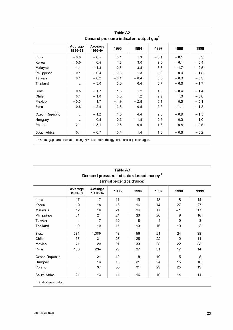
BIS Papers No 8 25

Table A2 Demand pressure indicator: output gap1

Average 1980-89

Average 1990-94 1995 1996 1997 1998 1999

India � 0.0 � 0.5 0.4 1.3 � 0.1 � 0.1 0.3 Korea � 0.0 � 0.5 1.5 3.0 3.9 � 6.1 � 0.4 Malaysia 1.1 � 1.3 0.5 3.8 6.6 � 4.7 � 2.5 Philippines � 0.1 � 0.4 � 0.6 1.3 3.2 0.0 � 1.8 Taiwan 0.1 � 0.2 � 0.1 � 0.4 0.5 � 0.3 � 0.3 Thailand .. � 3.0 3.0 6.4 3.7 � 6.6 � 1.7

Brazil 0.5 � 1.7 1.5 1.2 1.9 � 0.4 � 1.4 Chile 0.1 � 1.0 0.5 1.2 2.9 1.8 � 3.0 Mexico � 0.3 1.7 � 4.9 � 2.8 0.1 0.6 � 0.1 Peru 0.8 � 2.9 3.8 0.5 2.6 � 1.1 � 1.3

Czech Republic .. � 1.2 1.5 4.4 2.0 � 0.9 � 1.5 Hungary .. 0.8 � 0.2 � 1.9 � 0.8 0.3 1.0 Poland 2.1 � 3.1 0.8 0.9 1.6 0.8 � 0.5

South Africa 0.1 � 0.7 0.4 1.4 1.0 � 0.8 � 0.2 1 Output gaps are estimated using HP filter methodology; data are in percentages.

Table A3 Demand pressure indicator: broad money 1

(annual percentage change)

Average 1980-89

Average 1990-94 1995 1996 1997 1998 1999

India 17 17 11 19 18 18 14 Korea 19 18 16 16 14 27 27 Malaysia 12 18 21 24 17 � 1 17 Philippines 21 21 24 23 26 9 16 Taiwan .. 17 10 8 4 9 8 Thailand 19 19 17 13 16 10 2

Brazil 281 1,089 48 56 21 24 38 Chile 35 31 27 25 22 12 11 Mexico 71 29 21 33 28 22 23 Peru 180 294 29 37 31 17 14

Czech Republic .. 21 19 8 10 5 8 Hungary .. 13 18 21 24 15 16 Poland .. 37 35 31 29 25 19

South Africa 21 13 14 16 19 14 14 1 End-of-year data.

26 BIS Papers No 8

Table A4

Demand pressure indicator: unemployment rate1

Average 1990-94 1995 1996 1997 1998 1999

Korea 2 2 2 3 7 6 Malaysia 4 3 3 2 3 3 Philippines 9 10 9 9 10 10 Taiwan 2 2 3 3 3 3 Thailand 3 2 2 2 4 4

Brazil 5 5 5 6 8 7 Chile 6 5 6 6 6 10 Mexico 3 6 5 3 3 2 Peru 0 8 8 8 8 9

Czech Republic 3 3 3 4 6 9 Hungary 8 11 11 11 9 6 Poland 12 15 14 11 10 12 1 Yearly average in percentages.

Table A5 Cost pressure indicator: exchange rate1

(annual percentage change)

Average 1980-89

Average 1990-94 1995 1996 1997 1998 1999

India � 7 12 � 3 � 8 � 2 � 12 � 4 Korea � 3 � 4 4 � 4 � 15 � 32 18 Malaysia � 2 1 5 � 0 � 11 � 28 3 Philippines � 10 � 4 3 � 2 � 11 � 28 5 Taiwan 3 � 0 � 0 � 4 � 4 � 14 4 Thailand � 2 0 1 � 2 � 19 � 24 9

Brazil � 69 � 93 � 30 � 9 � 7 � 7 � 36 Chile � 18 � 9 6 � 4 � 2 � 9 � 10 Mexico � 37 � 6 � 47 � 16 � 4 � 13 � 4 Peru � 61 � 74 � 3 � 8 � 8 � 9 � 13

Czech Republic � 1 � 12 8 � 2 � 14 � 2 � 7 Hungary � 5 � 11 � 16 � 18 � 18 � 13 � 10 Poland � 34 � 42 � 6 � 10 � 8 � 6 � 12

South Africa � 11 � 6 � 2 � 16 � 7 � 17 � 10 1 A decline indicates a depreciation of the domestic currency.

BIS Papers No 8 27

Table A6 Cost pressure indicator: nominal wages1

Average 1990-94 1995 1996 1997 1998 1999

Korea 16 10 12 5 � 3 16 Malaysia 6 9 11 10 2 7 Philippines 6 2 12 15 6 7 Taiwan 9 3 5 4 1 6 Thailand 16 10 7 12 7 � 1

Brazil 1,453 72 20 6 Chile .. 13 14 9 8 6 Mexico 23 16 20 20 18 16 Peru � 10 2 3 76 11 � 3

Czech Republic 15 17 17 13 11 6 Hungary 22 20 23 22 15 11 Poland .. 33 27 21 16 10

South Africa 16 12 11 11 14 7 1 Annual percentage change of yearly averages.

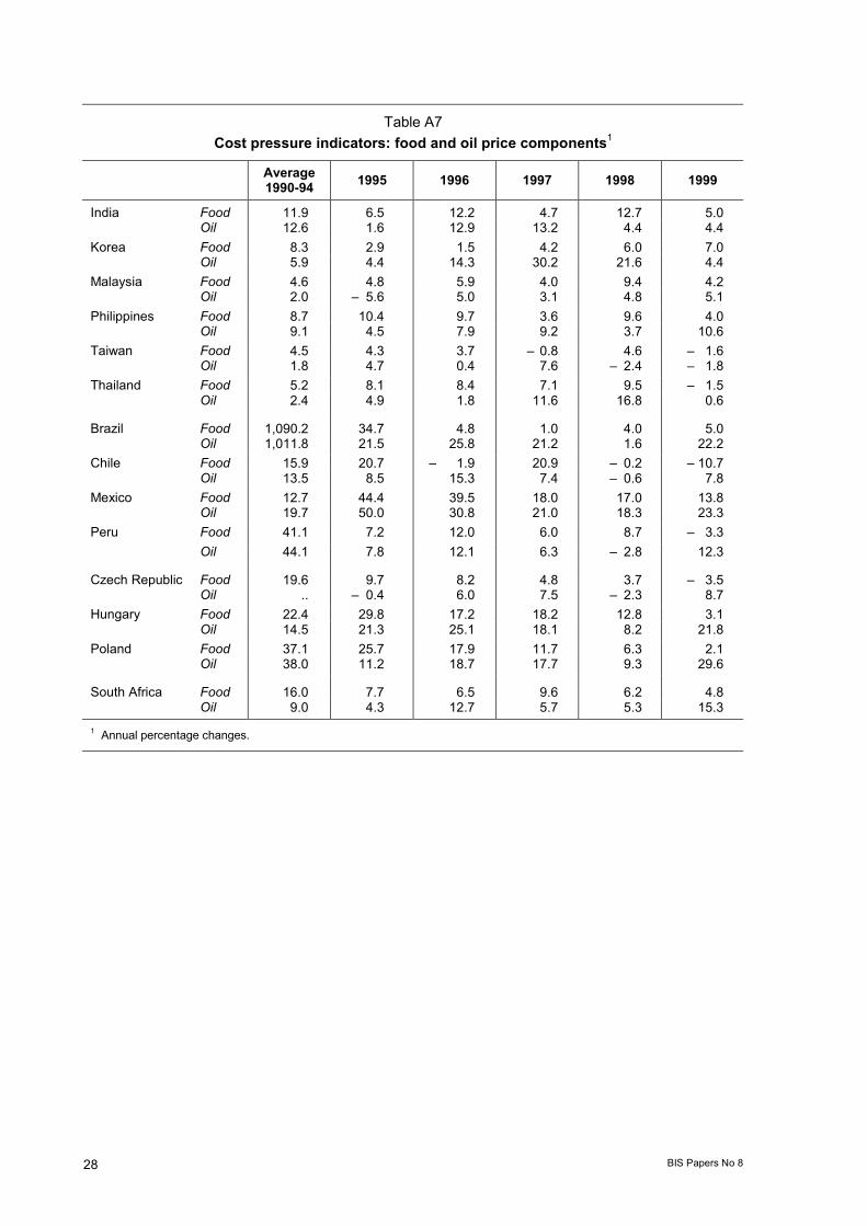
28 BIS Papers No 8

Table A7 Cost pressure indicators: food and oil price components1

Average 1990-94 1995 1996 1997 1998 1999

India Food 11.9 6.5 12.2 4.7 12.7 5.0 Oil 12.6 1.6 12.9 13.2 4.4 4.4 Korea Food 8.3 2.9 1.5 4.2 6.0 7.0 Oil 5.9 4.4 14.3 30.2 21.6 4.4 Malaysia Food 4.6 4.8 5.9 4.0 9.4 4.2 Oil 2.0 � 5.6 5.0 3.1 4.8 5.1 Philippines Food 8.7 10.4 9.7 3.6 9.6 4.0 Oil 9.1 4.5 7.9 9.2 3.7 10.6 Taiwan Food 4.5 4.3 3.7 � 0.8 4.6 � 1.6 Oil 1.8 4.7 0.4 7.6 � 2.4 � 1.8 Thailand Food 5.2 8.1 8.4 7.1 9.5 � 1.5 Oil 2.4 4.9 1.8 11.6 16.8 0.6

Brazil Food 1,090.2 34.7 4.8 1.0 4.0 5.0 Oil 1,011.8 21.5 25.8 21.2 1.6 22.2 Chile Food 15.9 20.7 � 1.9 20.9 � 0.2 � 10.7 Oil 13.5 8.5 15.3 7.4 � 0.6 7.8 Mexico Food 12.7 44.4 39.5 18.0 17.0 13.8 Oil 19.7 50.0 30.8 21.0 18.3 23.3 Peru Food 41.1 7.2 12.0 6.0 8.7 � 3.3 Oil 44.1 7.8 12.1 6.3 � 2.8 12.3

Czech Republic Food 19.6 9.7 8.2 4.8 3.7 � 3.5 Oil .. � 0.4 6.0 7.5 � 2.3 8.7 Hungary Food 22.4 29.8 17.2 18.2 12.8 3.1 Oil 14.5 21.3 25.1 18.1 8.2 21.8 Poland Food 37.1 25.7 17.9 11.7 6.3 2.1 Oil 38.0 11.2 18.7 17.7 9.3 29.6

South Africa Food 16.0 7.7 6.5 9.6 6.2 4.8 Oil 9.0 4.3 12.7 5.7 5.3 15.3 1 Annual percentage changes.

BIS Papers No 8 29

Table A8 Cost pressure indicator: import prices 1

Average 1990-94 1995 1996 1997 1998 1999

India 1.2 10.7 44.3 � 10.6 � 13.9 Korea � 0.7 9.0 � 0.4 � 9.3 � 17.8 � 3.1 Malaysia 1.6 � 0.7 0.0 15.3 16.2 � 0.5 Philippines � 1.4 1.3 4.5 2.4 3.3 � 7.0 Taiwan 1.6 11.9 � 1.0 1.1 0.3 2.6 Thailand � 1.4 12.7 12.4 24.4 11.0 � 8.6

Brazil � 3.4 2.3 � 9.7 6.5 � 5.3 0.3 Chile � 1.6 8.4 0.3 � 4.3 � 5.1 � 3.6 Mexico 1.5 5.4 0.1 0.7 � 1.0 � 0.6 Peru 1.6 6.5 3.3 � 3.7 � 4.5 2.3

Czech Republic 0.7 0.9 0.3 2.0 � 3.6 1.1 Hungary 19.7 31.1 21.0 13.6 11.4 5.5 Poland 20.9 18.4 13.9 11.9 3.0 7.4

South Africa 1.4 6.1 � 8.1 � 0.9 � 7.7 � 4.5 1 Annual percentage changes.

30 BIS Papers No 8

Table A9 Correlation with consumer price inflation

Food price

inflation Oil price inflation

Import price

inflation

Exchange rate

depreciationOutput

gap Broad money

expansionWage

increase Unemployment

rate

India 0.61 0.07 0.12 0.09 � 0.10 � 0.51 .. ..

Korea 0.50 � 0.06 � 0.12 0.47 0.15 � 0.45 0.06 � 0.20

Malaysia 0.71 � 0.11 � 0.10 0.22 � 0.13 � 0.26 � 0.40 0.21

Philippines 0.77 � 0.40 � 0.28 0.01 0.05 � 0.40 � 0.09 0.12

Taiwan 0.60 0.20 � 0.08 � 0.29 0.26 0.11 0.09 � 0.23

Thailand 0.71 0.33 0.42 0.36 0.43 0.27 .. � 0.29

Brazil 0.97 0.95 � 0.09 0.99 � 0.71 0.96 0.84 0.12

Chile 0.54 0.42 0.16 0.19 � 0.30 0.40 0.84 � 0.29

Mexico 0.96 0.64 0.30 0.66 � 0.46 0.75 0.88 0.26

Peru 0.71 � 0.05 � 0.04 � 0.28 0.36 0.31 � 0.05 0.19

Czech Republic 0.42 � 0.01 0.22 0.16 0.34 � 0.29 0.30 � 0.45

Hungary 0.78 0.34 0.76 0.48 � 0.19 � 0.56 0.10 0.40

Poland 0.84 � 0.20 0.36 � 0.02 0.02 0.23 0.70 0.73

South Africa 0.53 0.11 0.23 � 0.10 0.06 0.04 0.04 ..

BIS Papers No 8 31

0

15

30

45

60CPI 1 Output gap 2

0

15

30

45

60

0

10

20

30

40

0

10

20

30

40

1991 1993 1995 1997 1999

– 8

– 4

0

4

8

– 8

– 4

0

4

8

– 8

– 4

0

4

8

– 8

– 4

0

4

8

1991 1993 1995 1997 1999

Graph 1

1 Annual percentage change in consumer price index; left hand scale. 2 Right hand scale.

Brazil Chile

Mexico Peru

Czech Republic Hungary

Poland South Africa

Inflation and output gaps

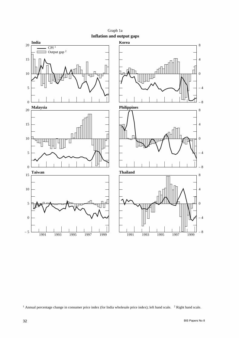
32 BIS Papers No 8

0

5

10

15

20CPI 1 Output gap 2

0

5

10

15

20

– 5

0

5

10

15

1991 1993 1995 1997 1999

– 8

– 4

0

4

8

– 8

– 4

0

4

8

– 8

– 4

0

4

8

1991 1993 1995 1997 1999

Graph 1a

1 Annual percentage change in consumer price index (for India wholesale price index); left hand scale. 2 Right hand scale.

India Korea

Malaysia Philippines

Taiwan Thailand

Inflation and output gaps

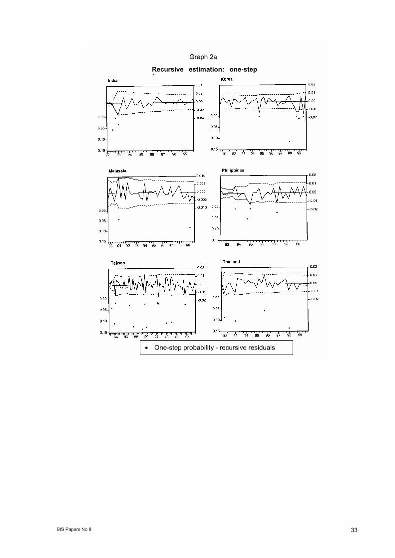
BIS Papers No 8 33

Recursive estimation: one-stepf t t t

Graph 2a

� One-step probability - recursive residuals

34 BIS Papers No 8

Recursive estimation: one-step forecast test

Graph 2b

� One-step probability - recursive residuals

BIS Papers No 8 35

Graph 2c

Recursive estimation: one-step forecast test

�� One-step probability - recursive residuals

36 BIS Papers No 8

Graph 3

Out-of-sample forecast

Note: Dynamic out-of-sample forecast over the period 1998-99.

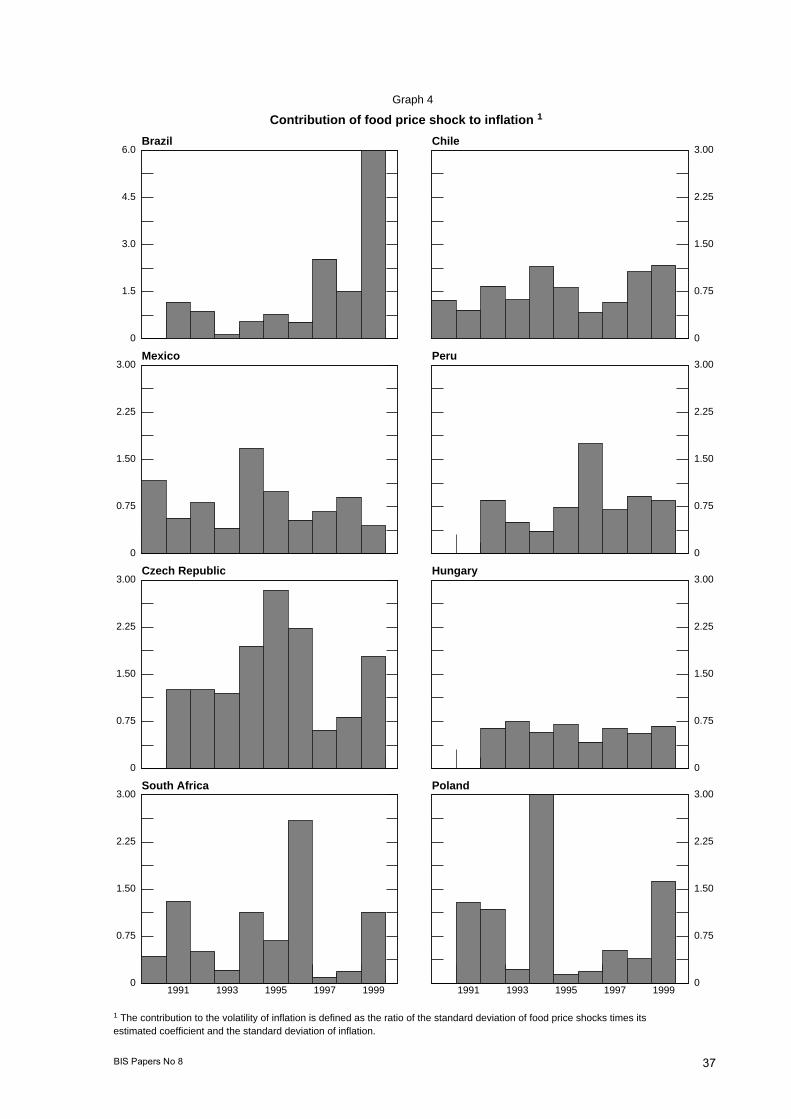
BIS Papers No 8 37

0

1.5

3.0

4.5

6.0

0

0.75

1.50

2.25

3.00

0

0.75

1.50

2.25

3.00

0

0.75

1.50

2.25

3.00

1991 1993 1995 1997 1999

0

0.75

1.50

2.25

3.00

0

0.75

1.50

2.25

3.00

0

0.75

1.50

2.25

3.00

0

0.75

1.50

2.25

3.00

1991 1993 1995 1997 1999

Graph 4

1 The contribution to the volatility of inflation is defined as the ratio of the standard deviation of food price shocks times itsestimated coefficient and the standard deviation of inflation.

Brazil Chile

Mexico Peru

Czech Republic Hungary

South Africa Poland

Contribution of food price shock to inflation 1

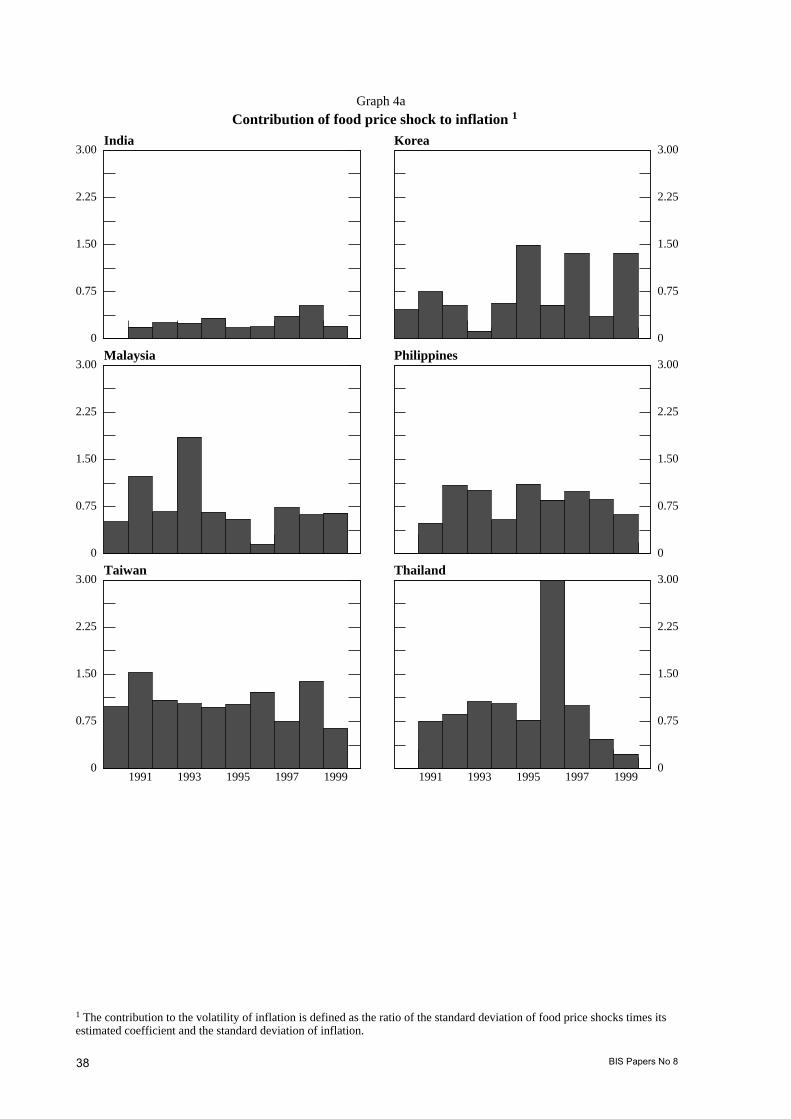
38 BIS Papers No 8

0

0.75

1.50

2.25

3.00

0

0.75

1.50

2.25

3.00

0

0.75

1.50

2.25

3.00

1991 1993 1995 1997 1999

0

0.75

1.50

2.25

3.00

0

0.75

1.50

2.25

3.00

0

0.75

1.50

2.25

3.00

1991 1993 1995 1997 1999

Graph 4a

1 The contribution to the volatility of inflation is defined as the ratio of the standard deviation of food price shocks times itsestimated coefficient and the standard deviation of inflation.

India Korea

Malaysia Philippines

Taiwan Thailand

Contribution of food price shock to inflation 1