what do cross-country studies teach about … · teach about government involvement, prosperity,...

JOEL SLEMROD University of Michigan

What Do Cross-Country Studies Teach about Government Involvement, Prosperity, and Economic Growth?

OVER THE LAST three decades, in all industrialized countries, there has been an enormous expansion of government involvement in the economy, as measured by the share of national income going to taxes or government expenditures. Figure 1 shows that, averaged over the OECD countries, the ratio of either tax collections or government expenditures to GDP rose sharply between 1970 and 1990. Arguably it is this expansion of government that uniquely characterizes the post- World War II era.

From the beginning, the growth in government has attracted critics who view this as an ominous development, endangering the political rights of the citizenry and economic prosperity. Leav-ing aside the issues of political freedom, this paper critically evaluates the evidence about the influence of government tax and expenditures on economic prosperity and growth.

It is worth pausing to reflect on what evidence would constitute support for the proposition that expanded government activity has been misguided. One option would be to assess the extent to which the goals of government expansion-provision of public goods, maintenance of full employment, insurance against social risks, income maintenance, and adequate provision of certain basic goods and services such as food, shelter, and medical care to all-have been achieved. Another would be to assess the cost, in terms of a lower average standard of living, of the programs designed to achieve this goal. Economists are a long way from consensus on measuring either the benefits or costs of government

I am grateful to Young Lee for expert research assistance; and to Edward Gramlich, Henry Ohlsson, Matthew Shapiro, Jonathan Skinner, Shlomo Yitzhaki, and members of the Brookings Panel for helpful comments on an earlier draft of this paper.

373

374 Brookings Papers on Economic Activity, 2:1995

Figure 1. Expenditure Ratio, Tax Ratio, and Real GDP Per Capita, OECD Countries, 1970-90a

Ratio 1990 dollars

0.450 - / DP per capita"o

0.425 - (right axis) - 18,000 Expenditure ratio"

0.400 _ (left axis)

__ ~~~~~~~~16,000 0.375-

0.350 - Tax ratio

/_ ........ .. . . @ (left axis) 0.325 - .

1970 1972 1974 1976 1978 1980 1982 1984 1986 1988 1990

Source: Expenditure and tax ratios (general goverrnment expenditure/GDP and general government tax revenue/GDP) are the author's calculations using data from International Monetary Fund ( 1994). Real GDP per capita is the author's calculation using the OECD's Nationail Accounts Statistics, 1994.

a. Twenty-four countries, excluding Mexico. b. Unweighted average, exchange rates and price levels of 1990. c. Unweighted average.

involvement. However, even a consensus on these two questions would not settle whether the big-government era has been a mistake, because weighing the benefits against the costs inevitably involves value judg- ments, about which economics is mute. This said, pinning down the cost is bound to be informative in the debate, because it can then, at least qualitatively, be stacked up against the benefits.

There are two approaches to measuring this cost: the "bottom-up" approach and the "top-down" approach. The bottom-up approach estimates cost country by country, program by program, and tax by tax. With all interactions among programs appropriately accounted for, the sum of these costs provides an estimate of the total cost of government involvement. There have been hundreds, perhaps thousands, of studies of the impact of particular government programs and tax features, fre- quently including an estimate of the associated economic cost.

There has been a much smaller, although growing, number of top- down studies, which investigate the association between a measure of the aggregate extent of government involvement and a measure of eco-

Joel Slemrod 375

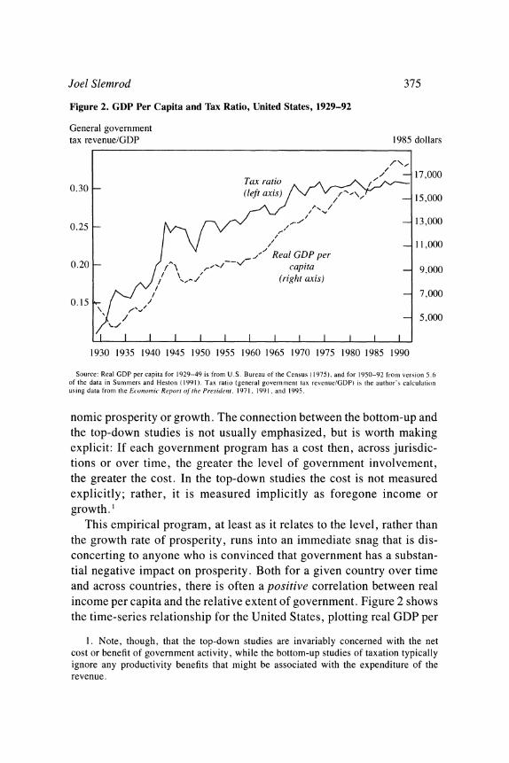
Figure 2. GDP Per Capita and Tax Ratio, United States, 1929-92

General government tax revenue/GDP 1985 dollars

Tax ratio 0.30 ~~~~~~~~~~~(left axis)

1,0

0.25 g / /_," 9 13,000

11,000 I , ~~~~Real GDP per

0.20 capita 9,000 ,J // \ - v (right axis)

7,000

) 5,000

1930 1935 1940 1945 1950 1955 1960 1965 1970 1975 1980 1985 1990

Source: Real GDP per capita for 1929-49 is from U.S. Bureau of the Census ( 1975), and for 1950-92 fronm version 5.6 of the data in Summers and Heston (1991). Tax ratio (general government tax revenue/GDP) is the author's calculation using data from the Economic Report of the Presidetnt, 1971, 1991, and 1995.

nomic prosperity or growth. The connection between the bottom-up and the top-down studies is not usually emphasized, but is worth making explicit: If each government program has a cost then, across jurisdic- tions or over time, the greater the level of government involvement, the greater the cost. In the top-down studies the cost is not measured explicitly; rather, it is measured implicitly as foregone income or growth. I

This empirical program, at least as it relates to the level, rather than the growth rate of prosperity, runs into an immediate snag that is dis- concerting to anyone who is convinced that government has a substantial negative impact on prosperity. Both for a given country over time and across countries, there is often a positive correlation between real income per capita and the relative extent of government. Figure 2 shows the time-series relationship for the United States, plotting real GDP per

1. Note, though, that the top-down studies are invariably concerned with the net cost or benefit of government activity, while the bottom-up studies of taxation typically ignore any productivity benefits that might be associated with the expenditure of the revenue.


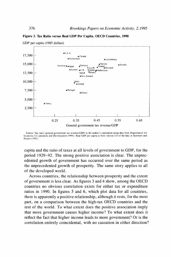
Figure 3. Tax Ratio versus Real GDP Per Capita, OECD Countries, 1990

GDP per capita (1985 dollars)

* U. S. A. 17,500 - Canada

* Switzerland * Luxembourg

15,000 - Germany *Norway .Sweden Australia. eJapan *Gray Finland France * * Denmark

* Iceland eU.K. Belgiumn Netherlands

12,500 Italy- *Austria *New Zealand

10,000 - Spain * Ireland

7,500 - . Portugal e Greece

5,000 - * Turkey

2,500 -

I I I II

0.25 0.35 0.45 0.55 0.65 General government tax revenue/GDP

Source: Tax ratio (general government tax revenue/GDP) is the author's calculation using data from Organisation for Economic Co-operation and Development (1994). Real GDP per capita is from version 5.6 of the data in Summers and Heston ( 1991).

capita and the ratio of taxes at all levels of government to GDP, for the period 1929-92. The strong positive association is clear. The unprecedented growth of government has occurred over the same period as the unprecedented growth of prosperity. The same story applies to all of the developed world.

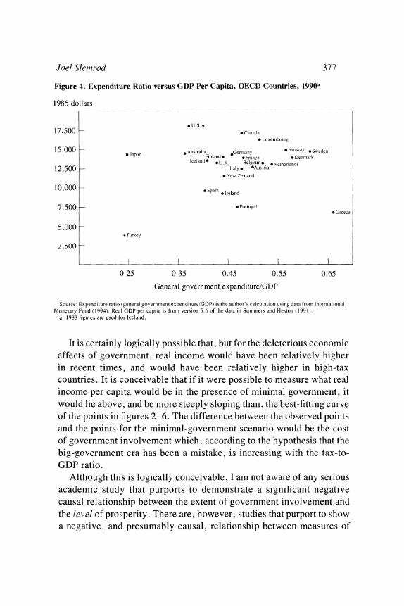
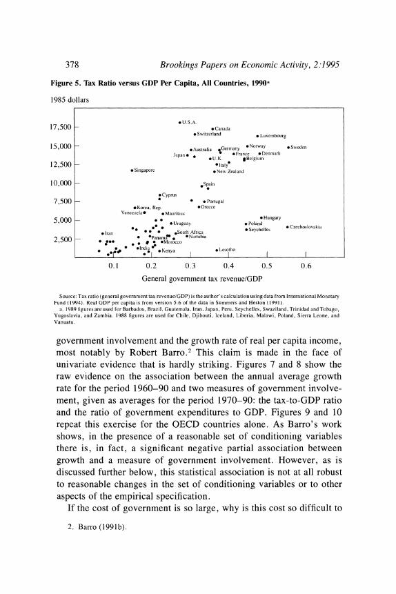
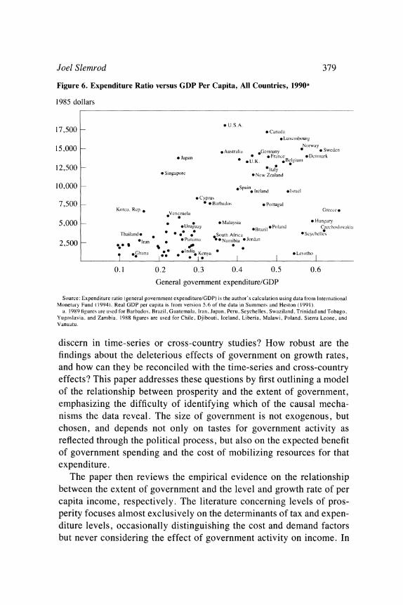
Across countries, the relationship between prosperity and the extent of government is less clear. As figures 3 and 4 show, among the OECD countries no obvious correlation exists for either tax or expenditure ratios in 1990. In figures 5 and 6, which plot data for all countries, there is apparently a positive relationship, although it rests, for the most part, on a comparison between the high-tax OECD countries and the rest of the world. To what extent does the positive association imply that more government causes higher income? To what extent does it reflect the fact that higher income leads to more government? Or is the correlation entirely coincidental, with no causation in either direction?

Joel Slemrod 377

Figure 4. Expenditure Ratio versus GDP Per Capita, OECD Countries, 199Oa

1985 dollars

* U.S.A. 17,500 . Canada

* Luxembourg

15,000 -Japan Australia Germnany eNorway *Sweden o Japan Finiande o ~~France e Denmark

Iceland0 *U .K. Belgiume. Netherlands

12,500 Italy * *Austria

* New Zealand

10,000 *Spain *Ireland

7,500 . Portugal * Greece

5,000 -

*Turkey

2,500 -

I I III 0.25 0.35 0.45 0.55 0.65

General government expenditure/GDP

Source: Expenditure ratio (general government expenditure/GDP) is the author's calculation using data from Internaltional Monetary Fund (1994). Real GDP per capita is from version 5.6 of the data in Summers and Heston (1991).

a. 1988 figures are used for Iceland.

It is certainly logically possible that, but for the deleterious economic effects of government, real income would have been relatively higher in recent times, and would have been relatively higher in high-tax countries. It is conceivable that if it were possible to measure what real income per capita would be in the presence of minimal government, it would lie above, and be more steeply sloping than, the best-fitting curve of the points in figures 2-6. The difference between the observed points and the points for the minimal-government scenario would be the cost of government involvement which, according to the hypothesis that the big-government era has been a mistake, is increasing with the tax-to- GDP ratio.

Although this is logically conceivable, I am not aware of any serious academic study that purports to demonstrate a significant negative causal relationship between the extent of government involvement and the level of prosperity. There are, however, studies that purport to show a negative, and presumably causal, relationship between measures of


Figure 5. Tax Ratio versus GDP Per Capita, All Countries, 1990a

1985 dollars

. U.S.A. 17,500 . Canada

* Switzerland * Luxembourg

15,000 -Australia Germany eNorway *Sweden Japan * *France * Denmark

eU.K. #Belgium 12,500 - * Italy

* Singapore * New Zealand

10,000 _ Spain

* Cyprus 7,500 * . Portugal

*Korea, Rep. oGreece Venezuela- * Mauritius

.5,000 -.0 * UHungary 0 * *Uruguay e Poland oCehsoai

*Iran South Africa *Seychelles *Czechoslovakia 2, 500 * *** PanamaZ. ONamibia

o o ;e *India * Kenya e Lesotho 00 ~~~~# O'D I o Kenya I ~~~~~~~~~~~~I II 0.1 0.2 0.3 0.4 0.5 0.6

General government tax revenue/GDP

Source: Tax ratio (general government tax revenue/GDP) is the author's calculation using data from International Monetary Fund ( 1994). Real GDP per capita is from version 5.6 of the data in Summers and Heston ( 1991).

a. 1989 figures are used for Barbados, Brazil, Guatemala, Iran, Japan, Peru, Seychelles, Swaziland, Trinidad and Tobago, Yugoslavia, and Zambia. 1988 figures are used for Chile, Djibouti, Iceland, Liberia, Malawi, Poland, Sierra Leone, and Vanuatu.

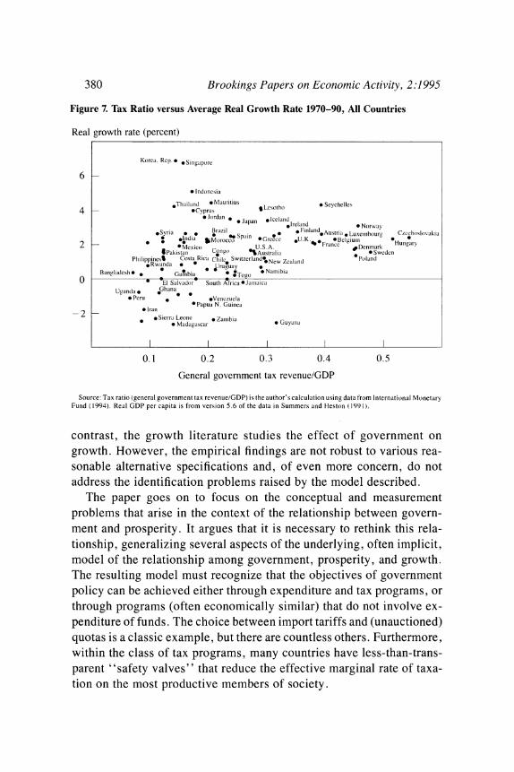
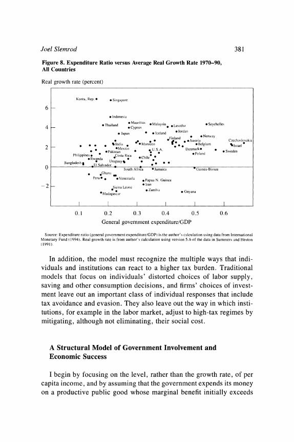
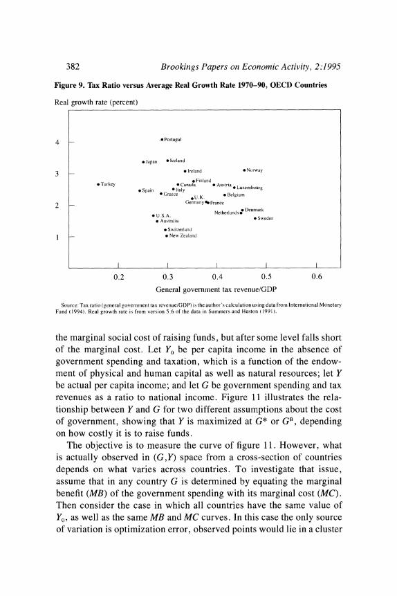
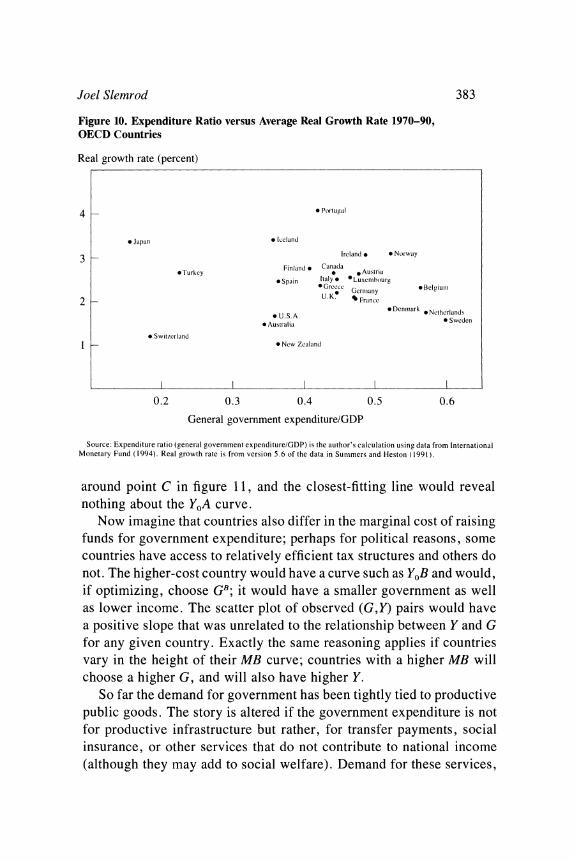
government involvement and the growth rate of real per capita income, most notably by Robert Barro.2 This claim is made in the face of univariate evidence that is hardly striking. Figures 7 and 8 show the raw evidence on the association between the annual average growth rate for the period 1960-90 and two measures of government involvement, given as averages for the period 1970-90: the tax-to-GDP ratio and the ratio of government expenditures to GDP. Figures 9 and 10 repeat this exercise for the OECD countries alone. As Barro's work shows, in the presence of a reasonable set of conditioning variables there is, in fact, a significant negative partial association between growth and a measure of government involvement. However, as is discussed further below, this statistical association is not at all robust to reasonable changes in the set of conditioning variables or to other aspects of the empirical specification.

If the cost of government is so large, why is this cost so difficult to

2. Barro (1991b).

Joel Slemrod 379

Figure 6. Expenditure Ratio versus GDP Per Capita, All Countries, 1990a

1985 dollars

U.SA. 17,500 . Canada

dLuxcmbourg

15,000 - ~~~~~~~~~~~~~~~~~~~Norway oSee 1Australia Gernlany r

o Swede * Japan * * Franc. i Denmark

*UK. *B3elgiunm

12,500 *ItaNe ly * S'ingapore * New Zealand

10,000 - *Spain * Ireland *Israel

* Cyprus

7,500 - * . B.,rbados . Portugal Korea. Rep. V Greece e

**Venczucla

5,000 - . Malayslia * Hungary *Uruguay 3raleoPoland Czecloslovakia

Thailand d * 0* *South Atrica *Seychelles

2,500 _* * *lr.n . ePanania *Narlibia eJordan

t %*&hana 1 n0 *India K * l Lesotho

0.1 0.2 0.3 0.4 0.5 0.6


Source: Expenditure ratio (general government expenditure/GDP) is the author's calculation using data fronm International Monetary Fund ( 1994). Real GDP per capita is from version 5.6 of the data in Summers and Heston (1991).

a. 1989 figures are used for Barbados, Brazil, Guatemala, Iran, Japan, Peru, Seychelles, Swaziland, Trinidad and Tobago, Yugoslavia, and Zanibia. 1988 figures are used for Chile, Djibouti, Iceland, Liberia, Malawi, Poland, Sierra Leone, and Vanuatu.

discern in time-series or cross-country studies? How robust are the findings about the deleterious effects of government on growth rates, and how can they be reconciled with the time-series and cross-country effects? This paper addresses these questions by first outlining a model of the relationship between prosperity and the extent of government, emphasizing the difficulty of identifying which of the causal mechanisms the data reveal. The size of government is not exogenous, but chosen, and depends not only on tastes for government activity as reflected through the political process, but also on the expected benefit of government spending and the cost of mobilizing resources for that expenditure.

The paper then reviews the empirical evidence on the relationship between the extent of government and the level and growth rate of per capita income, respectively. The literature concerning levels of prosperity focuses almost exclusively on the determinants of tax and expenditure levels, occasionally distinguishing the cost and demand factors but never considering the effect of government activity on income. In


Figure 7. Tax Ratio versus Average Real Growth Rate 1970-90, All Countries

Real growth rate (percent)

Korea. Rep.. *Singapore

6 * Indonesil

4, pThailand Maurilius Lesotho * Seychelles

0 Jordan * Japan 0Ieln *Syri * JarSpain IceanIreland * Norwaav

*Syria Braz'l

~~~~~* FinlandAuri Spain * W Brzi W Fnln'Austria * Luxerbour- Czechoslovaklia

2 _ * *India &Morocco P Greece *U.K.%* *nBelgiury

SPakistan Congo~~~~~~~~~Fa H ungary *Mexico U. S. A.Fac Denniark Pakistan Congo %Australia 0 Sweden

Philippines% CostRica ChileSwitzerland**NewZealOind * Rwanda

10 UrNeuZalndPaan * 0Jruuay Naniibia Bangladesh * Gambia *

:Togo 0 * El Salvador South Africa OJaittaica

Uganda * *Ghana * Peru .* Venezuela

0Iran * Papua N. Guinea *

*Sierra Leone * Zaittbia * Guyana *

Madagascar *Gyn

0.1 0.2 0.3 0.4 0.5


Source: Tax ratio (general government tax revenue/GDP) is the author's calculation using data from International Monetary Fund ( 1994). Real GDP per capita is from version 5.6 of the data in Summers and Heston ( 1991).

contrast, the growth literature studies the effect of government on growth. However, the empirical findings are not robust to various reasonable alternative specifications and, of even more concern, do not address the identification problems raised by the model described.

The paper goes on to focus on the conceptual and measurement problems that arise in the context of the relationship between government and prosperity. It argues that it is necessary to rethink this relationship, generalizing several aspects of the underlying, often implicit, model of the relationship among government, prosperity, and growth. The resulting model must recognize that the objectives of government policy can be achieved either through expenditure and tax programs, or through programs (often economically similar) that do not involve expenditure of funds. The choice between import tariffs and (unauctioned) quotas is a classic example, but there are countless others. Furthermore, within the class of tax programs, many countries have less-than-trans- parent "safety valves" that reduce the effective marginal rate of taxation on the most productive members of society.

Joel Slemrod 381

Figure 8. Expenditure Ratio versus Average Real Growth Rate 1970-90, All Countries


Korea, Rep.0 * Singapore

6 * Indonesia

4 _ . Thailand Mauritius * Malaysia . Lesotho * Seychelles 4 :~~~~~~~~~*Cyprus 0 ora

* Japan * Iceland *Jordan

* ** **Fiand Austria Czechoslovakia 10 00 o " 0 to 0

2 India i *Morocco * *Belgium %Israel 2 ~~~~~~~~OMexico *U. S. A. Denmarke * wee e Pakistan oln Swde

Philippines . Costa Rica *Chile * Rwanda Urugua hile

Bangladesh l Salgdo y *

,El Salvador 0 South Africa *jamaica Guinea-Bissau

* *Ghana Peru* eVenezuela *Papua N. Guinea

o *~~~~~~~~~~~~~~~~ Iran - 2 Sierra Leone

0. * Zambia * Guyana *oMadagascar

I I I l I I

0.1 0.2 0.3 0.4 0.5 0.6 General government expenditure/GDP

Source: Expenditure ratio (general government expenditure/GDP) is the author's calculation using data from International Monetary Fund ( 1994). Real growth rate is from author's calculation using version 5.6 of the data in Summers and Heston (1991).

In addition, the model must recognize the multiple ways that individuals and institutions can react to a higher tax burden. Traditional models that focus on individuals' distorted choices of labor supply, saving and other consumption decisions, and firms' choices of investment leave out an important class of individual responses that include tax avoidance and evasion. They also leave out the way in which institutions, for example in the labor market, adjust to high-tax regimes by mitigating, although not eliminating, their social cost.

A Structural Model of Government Involvement and Economic Success

I begin by focusing on the level, rather than the growth rate, of per capita income, and by assuming that the government expends its money on a productive public good whose marginal benefit initially exceeds


Figure 9. Tax Ratio versus Average Real Growth Rate 1970-90, OECD Countries


4 _.e Portugal

* Japan * Iceland

3 _ Ireland * Norway

* Finland * Turkey * Canada 0 Austria oLxmor r * Spain * Italy * Luxembourg

0 Greece *U.K * Belgium

2 Germany % France N Denmark

* U.S.A. Netherlandsj * Australia * Sweden

* Switzerland

l1 _ * New Zealand

0.2 0.3 0.4 0.5 0.6


Source: Tax ratio (general government tax revenue/GDP) is the author's calculation using data froni International Monetary Fund ( 1994). Real growth rate is from version 5.6 of the data in Summers and Heston ( 1991).

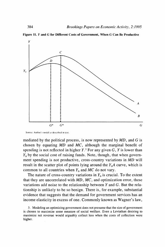
the marginal social cost of raising funds, but after some level falls short of the marginal cost. Let YO be per capita income in the absence of government spending and taxation, which is a function of the endowment of physical and human capital as well as natural resources; let Y be actual per capita income; and let G be government spending and tax revenues as a ratio to national income. Figure 11 illustrates the relationship between Y and G for two different assumptions about the cost of government, showing that Y is maximized at G* or GB, depending on how costly it is to raise funds.

The objective is to measure the curve of figure 11. However, what is actually observed in (G,Y) space from a cross-section of countries depends on what varies across countries. To investigate that issue, assume that in any country G is determined by equating the marginal benefit (MB) of the government spending with its marginal cost (MC). Then consider the case in which all countries have the same value of YO, as well as the same MB and MC curves. In this case the only source of variation is optimization error, observed points would lie in a cluster

Joel Slemrod 383

Figure 10. Expenditure Ratio versus Average Real Growth Rate 1970-90, OECD Countries


4 * Portugal

* Japan * Iceland

3 Ireland d eNorw,ay

Finland i Canada eTurkey * * Austria

eSpain Italy * *Luxenibourg *Grcc * Belgiuni * Gerniany

2 U. K. France

* Denimiark 0 Netherlands

0 USA.~rai 0 Sweden * Austraiia

* Switzerland 1 -*0 New Zealand

0.2 0.3 0.4 0.5 0.6


Source: Expenditure ratio (general government expenditure/GDP) is the author's calculation using data from International Monetary Fund ( 1994). Real growth rate is from version 5.6 of the data in Summers and Heeston ( 1991).

around point C in figure 11, and the closest-fitting line would reveal nothing about the YoA curve.

Now imagine that countries also differ in the marginal cost of raising funds for government expenditure; perhaps for political reasons, some countries have access to relatively efficient tax structures and others do not. The higher-cost country would have a curve such as YoB and would, if optimizing, choose GB; it would have a smaller government as well as lower income. The scatter plot of observed (G,Y) pairs would have a positive slope that was unrelated to the relationship between Y and G for any given country. Exactly the same reasoning applies if countries vary in the height of their MB curve; countries with a higher MB will choose a higher G, and will also have higher Y.

So far the demand for government has been tightly tied to productive public goods. The story is altered if the government expenditure is not for productive infrastructure but rather, for transfer payments, social insurance, or other services that do not contribute to national income (although they may add to social welfare). Demand for these services,


Figure 11. Y and G for Different Costs of Government, When G Can Be Productive

y

\ A

B

G' G* G

Sourcc: Author's imiodcl as describcd in text.

mediated by the political process, is now represented by MD, and G is chosen by equating MD and MC, although the marginal benefit of spending is not reflected in higher Y.3 For any given G, Y is lower than YO by the social cost of raising funds. Note, though, that when government spending is not productive, cross-country variations in MD will result in the scatter plot of points lying around the YoA curve, which is common to all countries when YO and MC do not vary.

The nature of cross-country variations in YO is crucial. To the extent that they are uncorrelated with MD, MC, and optimization error, these variations add noise to the relationship between Y and G. But the relationship is unlikely to be so benign. There is, for example, substantial evidence that suggests that the demand for government services has an income elasticity in excess of one. Commonly known as Wagner's law,

3. Modeling an optimizing government does not presume that the size of government is chosen to maximize some measure of social welfare. Even a Leviathan desiring to maximize net revenue would arguably collect less when the costs of collection were higher.

Joel Slemrod 385

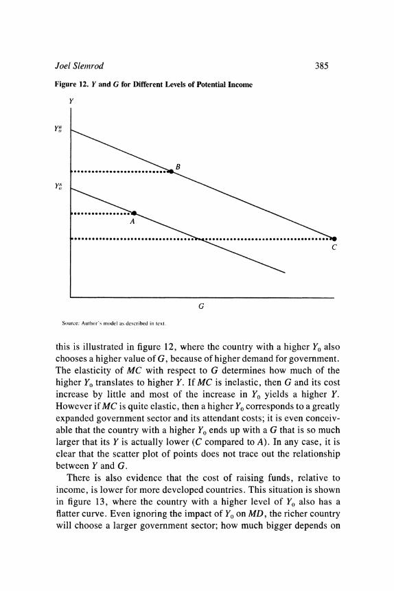
Figure 12. Y and G for Different Levels of Potential Income

y

G

Source: Author's model as described in text.

this is illustrated in figure 12, where the country with a higher YO also chooses a higher value of G, because of higher demand for government. The elasticity of MC with respect to G determines how much of the higher YO translates to higher Y. If MC is inelastic, then G and its cost increase by little and most of the increase in YO yields a higher Y. However if MC is quite elastic, then a higher YO corresponds to a greatly expanded government sector and its attendant costs; it is even conceivable that the country with a higher YO ends up with a G that is so much larger that its Y is actually lower (C compared to A). In any case, it is clear that the scatter plot of points does not trace out the relationship between Y and G.

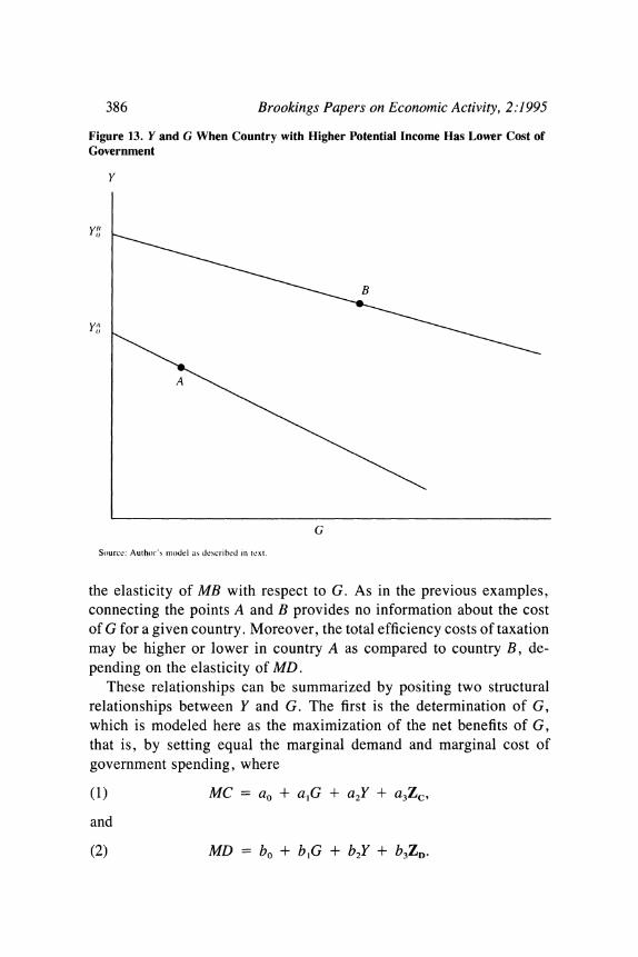
There is also evidence that the cost of raising funds, relative to income, is lower for more developed countries. This situation is shown in figure 13, where the country with a higher level of YO also has a flatter curve. Even ignoring the impact of YO on MD, the richer country will choose a larger government sector; how much bigger depends on


Figure 13. Y and G When Country with Higher Potential Income Has Lower Cost of Government

y

Y',

G

Source: Author's miiodel as described in text.

the elasticity of MB with respect to G. As in the previous examples, connecting the points A and B provides no information about the cost of G for a given country. Moreover, the total efficiency costs of taxation may be higher or lower in country A as compared to country B, depending on the elasticity of MD.

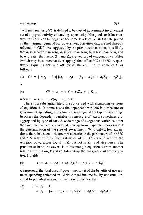
These relationships can be summarized by positing two structural relationships between Y and G. The first is the determination of G, which is modeled here as the maximization of the net benefits of G, that is, by setting equal the marginal demand and marginal cost of government spending, where

(1) MC=a, + a,G + a2Y+ a3Z,

and

(2) MD =bo+ blG + b2Y+ b3ZD.

Joel Slemrod 387

To clarify matters, MC is defined to be cost of government involvement net of any productivity-enhancing aspects of public goods or infrastructure; thus MC can be negative for some levels of G. MD is interpreted as the marginal demand for government activities that are not directly reflected in GDP. As suggested by the previous discussion, it is likely that a, is greater than zero, a2 is less than zero, b, is less than zero, and b2 is greater than zero. Zc and ZD are vectors of exogenous variables (which may be somewhat overlapping) that affect MC and MD, respectively. Equating MD and MC yields the equilibrium value of G as follows:

(3) G* = [1I(a, - b,)] [(bo' - a,) + (b2 - a2)Y + b3ZD - a3Zc],

or

(4) G* = co + clY + C2ZD + C3ZC

where cl = (b2 - a2)I(a, - b1) > 0. There is a substantial literature concerned with estimating versions

of equation 4. In some cases the dependent variable is a measure of government spending, sometimes disaggregated by type of spending. In others the dependent variable is a measure of taxes, sometimes disaggregated by type of tax. A wide range of exogenous variables other than income has been considered, arising from disparate theories about the determination of the size of government. With only a few exceptions, there has been little attempt to extricate the parameters of the MC and MD relationships from estimates of c1. This would require the isolation of variables found in Zc but not in ZD, and vice versa. The problem at hand, however, is to disentangle equation 4 from another relationship linking Y and G. Integrating the marginal cost from equation 1 yields

(5) C = a* + aoG + (a1/2)G2 + a2YG + a3ZcG.

C represents the total cost of government, net of the benefits of government spending reflected in GDP. Actual income is, by construction, equal to potential income minus these costs, so that

(6) Y= YO- C

- YO - [a* + aoG + (a /2)G2 + a2YG + a3ZcG].


Figure 14. Structural Relationships Linking Y and G

y

E

C~~~~~~

G


Positing that potential income is a linear function of a vector of endow- ments denoted W, so that

(7) YO = do + diW,

then the following relationship links Y and G:

(8) Y = do + djW - [a. + aoG + (a112)G2 + a2YG + a3ZcG],

or

(9) Y = 1/(1 + a2G) {do + djW - [a. + aoG + (a,/2)G2 + a3ZcG]}.

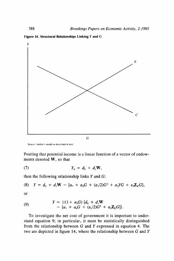
To investigate the net cost of government it is important to under- stand equation 9; in particular, it must be statistically distinguished from the relationship between G and Y expressed in equation 4. The two are depicted in figure 14, where the relationship between G and Y

Joel Slemrod 389

from equation 4 is labeled E, for equilibrium, and that from equation 9 is labeled C, for cost.

The best hope for estimating equation 9 is to find variables that are contained in ZD but not in Zc. These determinants of the "demand" for government will shift the E curve but not the C curve, thus tracing out the C curve. As discussed further below, finding any such variable is problematic. In the absence of such variables it is impossible to know how to interpret scatter plots like those of figures 3-6 because they do not, by themselves, clearly reveal the cost, if any, of government activity. More sophisticated analysis is required.

Empirical Analyses of the Relationship between Government and Prosperity

There is a vast empirical literature investigating the relationship between the extent of government and the level of prosperity. Little of it makes any reference at all to the structural relationships that link the two; an exception is the work of Bruce Bolnick, who analyzes tax patterns across countries in a simultaneous model, including demand factors such as the dependency ratio and per capita income and also supply factors proxying for the ease of tax collection.4 No one has had the temerity to regress Y against a set of variables that includes measures of G, perhaps because of the daunting challenge of identifying variables in the vector W, and perhaps also because of the courage needed to assert that no important unmeasured influences on Y would be correlated with G.5

There have, however, been scores of empirical studies by economists, political scientists, and sociologists that try to explain G or the growth of G, some of which include Y as a regressor. The conceptual models underlying the studies vary widely; the following discussion gives only a flavor of the approaches.

Writing in 1883, Adolph Wagner proposed the law of expanding state activity, which, in modern terminology, posits that citizens' demand for government-provided goods and services is income-elastic,

4. See Bolnick (1978). 5. As discussed below, the growth of Y has quite often been regressed on G, espe-

cially in recent years.


due to the "pressure for social progress" and the need for infrastructure investments. Jack Peacock and Jack Wiseman stress instead the importance of crises such as war and depressions, arguing that the greater role of government during these times increases the tolerable burden of taxation. This remains high after the crisis has passed, both because the expanded bureaucracy is better able to assert its interests and because war, in particular, concentrates power at the national level. This theory, however, is unable to explain the large rise in the role of the public sector after World War II. William Baumol argues that the labor- intensive nature of government services, with the attendant lagging productivity growth, implies that their relative price is bound to increase over time. As a result, the share of government in GDP will increase, as long as demand is less than unit-elastic.6

Another set of theories has emphasized the political mechanism that maps individuals' preferences into outcomes. One example is the collective choice model, in which politicians cater to the median voter, as illustrated by Theodore Bergstrom and Robert Goodman. James Buch- anan and Richard Wagner argue that, because of its nature as a public good and its uncertain benefits, much of government spending will be provided suboptimally unless the tax burden is concealed by means of value added or sales taxes, creating a "fiscal illusion." William Nis- kanen stresses the role of bureaucracies that value larger budgets and have the power to extract budget dollars from the legislature. Samuel Peltzman argues that the incentive to redistribute wealth politically, not the demand for public goods, is the most important determinant of the relative size and growth of government, and that the growth of the middle class has been a major source of government growth in the developed world since 1930.7

The eminent public finance economists Richard Goode and Richard Musgrave note the high positive correlation, over time and across countries, between GDP per capita and total tax ratios.8 Goode suggests that rather than income being the driving factor, this correlation may result from the positive correlation between per capita income and other social and economic conditions that make direct taxes acceptable and effec-

6. See Wagner (1883), Peacock and Wiseman (1961), and Baumol (1967). 7. See Bergstrom and Goodman (1973), Buchanan and Wagner (1977), Niskanen

(1971), and Peltzman (1980). 8. See Goode (1968) and Musgrave (1969).

Joel Slemrod 391

tive, such as a high level of literacy, wide use of standard accounting methods, effective public administration, and political stability.

A recent example of this empirical literature is the work of Vito Tanzi, who investigates the determinants of the share of tax in GDP in eighty-three developing countries for several years during the period 1978-88.9 By itself, the log of per capita income is positively associated with the tax ratio, although both the estimated coefficient and its associated t statistics are less than half their size in the 1988 regression compared to the 1978 regression. He goes on to show that the share of agricultural output in total GDP, an important element of the Z4 vector, explains more of the variation in tax shares than does per capita income and has a negative sign. Where both variables are included, per capita income no longer has a significant positive effect, although the negative effect of the agricultural share survives; as Tanzi notes, these two variables are highly negatively correlated.

The results of Goode and Tanzi can be restated in the language of the model presented above. They observe that c,Y from equation 4 is positive. They ascribe this not to a positive value of b2, but to a negative value of a2. However, they suggest that the negative value of a2 would fall to zero, or close to zero, if the elements of Zc, conditions that facilitate the use of efficient means of efficient tax regimes that are highly positively correlated with Y, could be adequately measured. They do not consider any feedback effect of G on Y, such as that in equation 6.

Empirical Analyses of the Relationship between the Growth of Government and Income Growth

In recent years there has been an explosion of top-down, cross- country studies of the impact of government taxation and expenditure. There are two striking differences between the recent crop of studies and those surveyed above. First, the G variable is always on the right- hand, rather than left-hand, side of the regression equation, and little or no attention is paid to how it is determined. Thus equation 6, alone, is investigated, without reference to equation 4. Second, in all cases

9. See Tanzi (1992).


the dependent variable of equation 6 is a measure, not of the level of prosperity but rather, of its rate of growth.

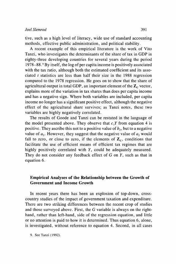
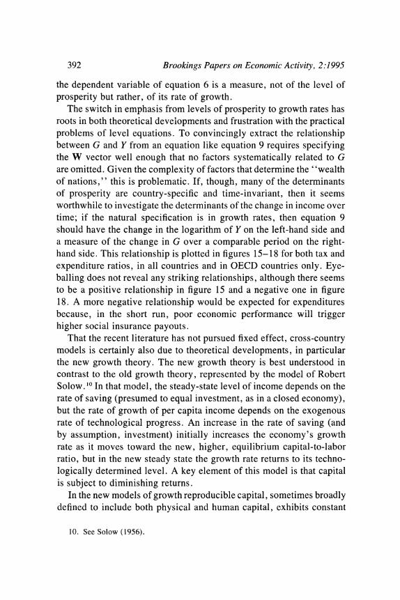
The switch in emphasis from levels of prosperity to growth rates has roots in both theoretical developments and frustration with the practical problems of level equations. To convincingly extract the relationship between G and Y from an equation like equation 9 requires specifying the W vector well enough that no factors systematically related to G are omitted. Given the complexity of factors that determine the "wealth of nations," this is problematic. If, though, many of the determinants of prosperity are country-specific and time-invariant, then it seems worthwhile to investigate the determinants of the change in income over time; if the natural specification is in growth rates, then equation 9 should have the change in the logarithm of Y on the left-hand side and a measure of the change in G over a comparable period on the right- hand side. This relationship is plotted in figures 15-18 for both tax and expenditure ratios, in all countries and in OECD countries only. Eye- balling does not reveal any striking relationships, although there seems to be a positive relationship in figure 15 and a negative one in figure 18. A more negative relationship would be expected for expenditures because, in the short run, poor economic performance will trigger higher social insurance payouts.

That the recent literature has not pursued fixed effect, cross-country models is certainly also due to theoretical developments, in particular the new growth theory. The new growth theory is best understood in contrast to the old growth theory, represented by the model of Robert Solow. 10 In that model, the steady-state level of income depends on the rate of saving (presumed to equal investment, as in a closed economy), but the rate of growth of per capita income depends on the exogenous rate of technological progress. An increase in the rate of saving (and by assumption, investment) initially increases the economy's growth rate as it moves toward the new, higher, equilibrium capital-to-labor ratio, but in the new steady state the growth rate returns to its techno- logically determined level. A key element of this model is that capital is subject to diminishing returns.

In the new models of growth reproducible capital, sometimes broadly defined to include both physical and human capital, exhibits constant

10. See Solow (1956).

Figure 15. Change in Tax Ratio 1970-74 to 1985-89 versus Average Real Growth Rate 1970-89, All Countriesa

Real growth rate (percent) 8

Singapore * Korea, Rep.

6 Malta

0 0~~~~~ Botswana Indonesia * *Mauritius * Lesotho Jordan Yemen 4 * *Thailand *Cyprus

Iceland * Japan * Portugal * Finland

2 Egypt S * tdi 1 1 * Indi'* Luxembourg

2 * . ~~~~~~~~ ~~~~~~~~*Israel * U. S. A. 9 *Denmark *Sweden

*Nigeria o Chile **Switzerland

S Oman Uruguay. * sCosta Rica eTogo * S Rana *Zimbabwe

South Atrica * Jamaica

*Suriname *Papua N. Guinea *Venezuela

-2 Zambia Iran *Sierra Leone . G

* Madagascar *Guyana

-0.1 0 0.1 0.2 Change in tax ratio

Source: Tax ratio (general government tax revenue/GDP) is the author's calculation using data from International Monetary Fund ( 1994). Real growth rate is from version 5.6 of the data in Summers and Heston ( 1991).

a. Change in tax ratio is calculated as change from 1970-74'average to 1985-89 average.

Figure 16. Change in Expenditure Ratio 1970-74 to 1985-89 versus Average Real Growth Rate 1970-89, All Countriesa


Korea, Rep. *Singapore

6 *Malta * *Mauritius *Botswana

Thailand Malaysia *Yemen 4 - .Jordan * *Cyprus * Iceland eJapan * *Portugal

* * Finland Luxembourg 0 0 0 ~ *0 0 ettaly

2 Go . U. S.A India eDnmark *Francc Greece * * e * * * * Sweden

*Chile e Nigeria *New Zealand Oo Uruguay | * rica *Zimbabwc o *~~~~ ~ ~~~~~Togo *

0 0 0 *~~~~~~~~~~~~~~~~Jamaica

*Uganda *Papua N. Guinea *Suriname * Ghana *Venezuela

-2 .Iran *Sierra Leone * Zambia *Chad

Madagascar

-0.1 0 0.1 0.2 Change in expenditure ratio

Source: Expenditure ratio (general government expenditure/GDP) is the author's calculation using data from International Monetary Fund (1994). Real growth rate is from version 5.6 of the data in Summers and Heston ( 1991).

a. Change in expenditure ratio is calculated as change from 1970-74 average to 1985-89 average.

Figure 17. Change in Tax Ratio 1970-74 to 1985-89 versus Average Real Growth Rate 1970-89, OECD Countriesa


Iceland . * Portugal

3.5- * Japan

* Norway

3.0 C .Finland Canada o

* Ireland

* Austria Italy. * Luxembourg

2.5 .-UKGreece eSpain Turkey * * U.K * Belgium

2.5 -* Germany * France

U.S.A. * Denmark * Netherlands * Australia * Sweden

1.5 -

New Zealand 0 * Switzerland

. _ _ _ _ _ . _ _ . _ I I

0 0.1 0.2 Change in tax ratio

Source: Tax ratio (general government tax revenue/GDP) is the author's calculation using data from International Monetary Fund (1994). Real growth rate is from version 5.6 of the data in Summers and Heston (1991).

a. Change in tax ratio is calculated as change from 1970-74 average to 1985-89 average.

Figure 18. Change in Expenditure Ratio 1970-74 to 1985-89 versus Average Real Growth Rate 1970-89, OECD Countriesa


3.5 - . Iceland 0 Portugal

*Japan

* Norway

3.0 C-nda. Finland 3.0 _ ~~~~~~~~~~~~Canada 9

* Ireland

2.5 _ * Austria * Luxembourg * Italy U. K. e Spain Greece

* * Turkey * Belgium

2.0 - . Germany 0 France

U.S.A.0 Denmark

Netherlands *Australia * Sweden

1.5 -

* New Zealand _ _ _ _ _ _ _ _ _ _ _, II

0 0.1 0.2 Change in expenditure ratio

Source: Expenditure ratio (general government expenditure/GDP) is the author's calculation using data from International Monetary Fund ( 1994). Real growth rate is from version 5.6 of the data in Summers and Heston ( 1991).

a. Change in expenditure ratio is calculated as change from 1970-74.average to 1985-89 average.

Joel Slemrod 395

returns to scale. One class of models achieves this by introducing external effects of capital either because, as in that of Robert Lucas, human capital makes other workers more productive or, as in that of Paul Romer, the aggregate stock of knowledge provides an externality. Another class of model, due to Sergio Rebelo, posits that all inputs to the production process are some form of reproducible capital, and that output can be expressed as a linear function of this broad concept of capital. These models share the implication that, because there are no diminishing returns to capital accumulation, a constant rate of investment, by increasing the capital stock, steadily increases output. A one- time increase in the investment-to-output ratio therefore increases the economy's growth rate forever because it increases the rate of capital accumulation forever. "I

The policy implications are clear. The welfare consequences of any influence on the accumulation of capital or the stock of knowledge loom much larger than in old growth models. And as William Easterly and Rebelo point out, "it is hard to think of an influence on the private real rate of return and on the growth rate that is more direct than that of income taxes. If these do not affect the rate of growth, what does?"'2 Robert King and Rebelo offer a striking example of the theoretical potency of income taxes. 13 They simulate the effects of increasing the income tax rate from 20 percent to 30 percent; this lowers the after-tax return to capital accumulation, and the saving rate. By lowering the growth rate from 2.00 percent to 0.37 percent, the loss in welfare is equivalent to a permanent drop of 65 percent in real consumption. In the Solow model, the same tax experiment causes a welfare loss equivalent to a permanent drop of 1.6 percent in real consumption.

The combination of new theories of growth and the recent availability of an abundance of comparable cross-country data, due to the work of Robert Summers and Alan Heston, triggered a renaissance of empirical studies of the determinants of growth. In the most influential of these studies, Barro examines a cross-section of ninety-eight countries for the period 1960-85 and, among other concerns, investigates how economic growth is affected by government expenditures, measured as the ratio of real government consumption purchases less spending on edu-

1 1. See Lucas (1988), Romer (1990), and Rebelo (1991). 12. Easterly and Rebelo (1993, p. 418). 13. See King and Rebelo (1990).


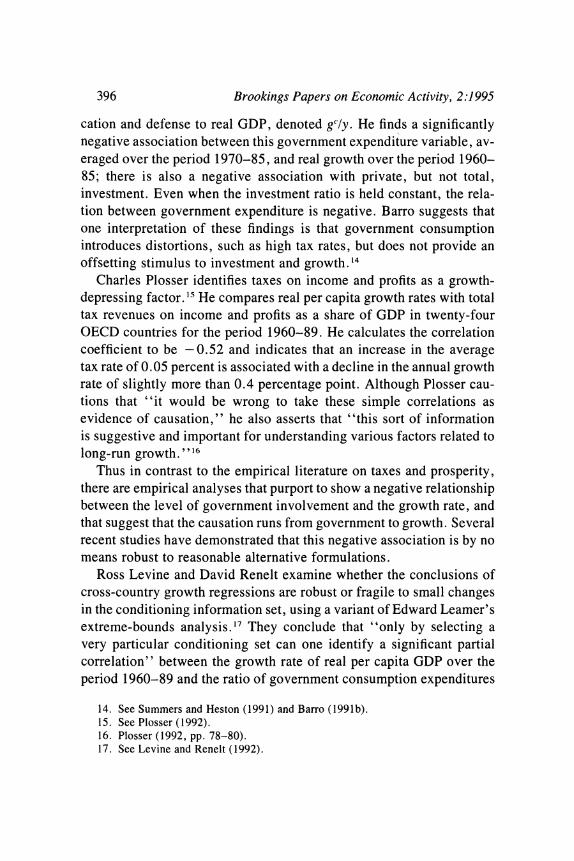
cation and defense to real GDP, denoted gC/y. He finds a significantly negative association between this government expenditure variable, averaged over the period 1970-85, and real growth over the period 1960- 85; there is also a negative association with private, but not total, investment. Even when the investment ratio is held constant, the relation between government expenditure is negative. Barro suggests that one interpretation of these findings is that government consumption introduces distortions, such as high tax rates, but does not provide an offsetting stimulus to investment and growth.'4

Charles Plosser identifies taxes on income and profits as a growth- depressing factor. '5 He compares real per capita growth rates with total tax revenues on income and profits as a share of GDP in twenty-four OECD countries for the period 1960-89. He calculates the correlation coefficient to be -0.52 and indicates that an increase in the average tax rate of 0.05 percent is associated with a decline in the annual growth rate of slightly more than 0.4 percentage point. Although Plosser cau- tions that "it would be wrong to take these simple correlations as evidence of causation," he also asserts that "this sort of information is suggestive and important for understanding various factors related to long-run growth."''6

Thus in contrast to the empirical literature on taxes and prosperity, there are empirical analyses that purport to show a negative relationship between the level of government involvement and the growth rate, and that suggest that the causation runs from government to growth. Several recent studies have demonstrated that this negative association is by no means robust to reasonable alternative formulations.

Ross Levine and David Renelt examine whether the conclusions of cross-country growth regressions are robust or fragile to small changes in the conditioning information set, using a variant of Edward Leamer's extreme-bounds analysis.'7 They conclude that "only by selecting a very particular conditioning set can one identify a significant partial correlation" between the growth rate of real per capita GDP over the period 1960-89 and the ratio of government consumption expenditures

14. See Summers and Heston (1991) and Barro (1991b). 15. See Plosser (1992). 16. Plosser (1992, pp. 78-80). 17. See Levine and Renelt (1992).

Joel Slemrod 397

to GDP. 8 Nor is there a robust relationship between growth and the ratio of total government expenditures to GDP, or between growth and government consumption expenditures excluding education and defense expenditures, which is the measure of government economic involvement used by Barro; the coefficient on Barro's government variable becomes insignificant when Levine and Renelt include the ratio of exports to GDP and the standard deviation of domestic credit growth in the conditioning set. '9 Nor are disaggregated measures of government activity-the ratio to GDP of government capital formation, government education expenditures, and government defense expenditures- robustly correlated with growth rates. Moreover, none of these fiscal policy indicators is robustly correlated with the investment share of GDP, one of the few variables that survives the extreme-bounds analysis test of a robust relationship with growth.

Jonas Agell, Thomas Lindh, and Henry Ohlsson also conclude that the relationship between growth and the ratio of taxes or expenditures to GDP is not robust. Focusing on the OECD countries only, they show that simply adding two demographic variables concerning dependency ratios (the fraction of the population younger than fifteen, and the fraction older than sixty-four) to the estimating equation is enough to turn a negative partial relationship between growth and government into a positive, albeit insignificant, one.20

Easterly and Rebelo perform a careful analysis of the effect of fiscal policy on economic growth, using several different measures of fiscal policy. They find that measures of the level of taxes tend to be insignificant in Barro's type of growth rate regression, often causing the coefficient on initial income to become statistically insignificant as well. The authors ascribe this finding to the strong positive correlation between their fiscal variables and the initial (1960) level of per capita income, making it difficult to disentangle the effects of fiscal variables from those of the initial level of income. This is the convergence effect discussed by Barro and Xavier Sala-i-Martin, and others. Of the thirteen tax variables they investigate, only one is (barely) significant at the 5

18. Levine and Renelt (1992, p. 951). 19. See Barro (1991b). 20. See Agell, Lindh, and Ohlsson (1995).


percent level-the "marginal" income tax computed with individual country time series to regress income tax revenue on GDP.21

Easterly and Rebelo argue that the same problem applies to the negative correlation between growth and the income tax share of GDP among OECD countries presented by Plosser-when the initial level of income is controlled for, the negative relation between these two variables disappears.22 They conclude that, in contrast to the robustness of theoretical predictions, "the evidence that tax rates matter for growth is disturbingly fragile."23

Jean-Louis Arcand and Marcel Dagenais explore the implications of errors in the variables commonly used in cross-country regressions.24 Rather than using ordinary least squares (OLS), they use a "higher- moments" estimator that they claim is robust, under quite reasonable assumptions, to errors in variables. They highlight equation 1 of Barro's study, in which their reestimation of the OLS coefficient on gc/y yields -0.0818, with a standard error of 0.0226. Using their estimator, this coefficient is -0.03 19, with a standard error of 0.0510. They conclude that "while this does not mean that the government consumption expenditures have no negative impact on the growth rate, it does raise doubts about the 'stylized fact' proposed by Barro . . . and suggests that more carefully constructed data on government consumption expenditures is needed before one can pronounce oneself one way or the other.' '25 Moreover, with their estimator the effect of gc/y on the investment ratio becomes less negative, and in two versions of Barro's specification it becomes positive and statistically significant at the usual levels of confidence.

Even this cursory review makes clear that the partial cross-country association between growth and measures of government involvement is not robust to several aspects of the empirical specification. This may not be too surprising, given the difficult problems of measuring the extent of government involvement which are discussed further, below.

There is a striking contrast between the statistical explorations of the relationship between G and the level of Y and those that investigate the

21. See Easterly and Rebelo (1993, pp. 426-27), and Barro and Sala-i-Martin (1992).

22. See Plosser (1992). 23. Easterly and Rebelo (1993, p. 442). 24. See Arcand and Dagenais (1994). 25. Arcand and Dagenais (1994, p. 19) on Barro (1991b).

Joel Slemrod 399

link between G and the growth rate of Y. The level studies primarily try to explain G and often include Y as one explanatory variable; that G might affect Y is ignored, as is (with some exceptions) the structural interpretation of the effect of Y on G. The growth studies try to explain the growth rate of Y (henceforth AY) and often include G as one of the explanatory variables. The possibility of a structural relationship determining G is often completely ignored.

Barro's work is a clear exception to the last statement, as it addresses sorne of the issues raised in describing the model above.26 Although the conceptual model underpinning Barro's empirical analysis is quite different, the statistical issues can be illustrated using the model given here. First, he recognizes that if governments are optimizing and countries differ only in the relative productivity of government services, then the covariation between G and AY does not correspond to a relationship like equation 9 and "there would not be much cross-country relation between growth rates and the size of government. "27

This problem leads Barro to the effect of government consumption expenditures, which, in his model, should unambiguously lead to lower growth rates because they do not enter private production functions.28 He then argues that in this case the remaining problem of interpretation stems from Wagner's law-that higher levels of income lead to an increase in g'/y.29 Given the initial level of income, a higher growth rate leads to higher average income over the sample and hence, a higher value of g'/y. This amounts to recognizing the problem of separately identifying equations 4 and 6. Barro concludes that spurious correlation associated with Wagner's law is a problem for government transfers, but not for government consumption, investment, or education expenditures, and he therefore enters measures of these activities separately into a growth rate regression.30 This conclusion about potential spurious correlation rests on the finding that only for transfers for social insurance and welfare (out of five spending categories) does the level of income in 1960 account for a substantial fraction of the cross-country

26. See Barro (1991a). 27. Barro (1991a, p. 278). 28. See Barro (1991b). 29. See Barro (199la). 30. If the reason that government expenditures have negative economic conse-

quences is the taxes that are required to support them, then the total cost (deadweight loss) depends on the sum of taxes raised, not on the expenditure components.


variance in the spending ratio; however, both government consumption and education expenses are significantly correlated with per capita income in 1960; negatively and positively, respectively.

This exercise in no way disposes of the problems of interpreting the coefficient in a growth equation on a measure of government involvement, because even for nonproductive expenditures there is likely to be a relationship between the optimal size of government and the contribution to prosperity of government. Alternatively if, as most public finance economists have concluded, there are important cross-country differences in the cost of mobilizing resources for government, then unmeasured variation in this factor will cause the scatter plot not to approximate the C curve of figure 14. This will be true as long as the level of government activity chosen by a country depends on the economic cost of mobilizing resources to fund the activity, a weak assertion indeed. What is required is to create an instrument for G using indicators of MD, that is, elements of the vector ZD that are not also in Zc. As stated earlier, this is a difficult task because many of the obvious elements of ZD, such as the extent of urbanization, are also found in Zc.

Because these issues have not yet been dealt with adequately, it is not advisable to interpret the estimated coefficient on a G variable to represent the cost of government.3' Moreover, there are further problems of interpretation because many of the key variables in the W vector are also likely to be in the Zc vector. Consider measures of the human capital endowment of a country, the critical element of several new growth models. In a more prosaic vein, a more educated citizenry is a key requirement for implementing arguably more efficient direct (income) taxes; in other words, more human capital (H) not only raises Y0 because it is an element of W, but also reduces MC because it is an element of Zc. The coefficient on H in a reduced-form equation ex- plaining Y, or AY, reflects not only its direct effect on potential income through W, but also the fact that higher H reduces the slope of the C curve and shifts the E curve to the right, which has an additional effect on Y, of ambiguous sign.

31. Engen and Skinner (1992), noting potential problems of endogeneity, use instruments for fiscal policy variables (the change in tax and expenditure shares), but make no attempt to differentiate the Zc vector from the ZD vector and, in fact, explicitly include as instruments variables measuring the ease of tax collection, such as the literacy rate and the percentage of the population that is urbanized.

Joel Slemrod 401

This review of the existing cross-country literature suggests that there is no persuasive evidence that the extent of government has either a positive or a negative impact on either the level or the growth rate of per capita income, largely because the fundamental problems of identification have not yet been adequately addressed. This does not imply that there are no examples of programs or taxes that do have an important effect; bottom-up studies must be the source of such conclusions. The next section investigates some conceptual issues that arise in relat- ing the bottom-up and top-down studies of the effect of taxes on economic outcomes. It explores the possible reasons why top-down studies might find a negligible effect, and whether this finding is compatible with a significant behavioral response to tax disincentives.

Reassessing the Relationship between Government and Prosperity

One possible explanation for a negligible aggregate relationship between the level of government and prosperity is that the compensated behavioral response, and therefore distortion, due to the relative price changes caused by taxes is not very large. This is not the place to review the vast bottom-up empirical literature, but it is fair to say that there remains substantial controversy about such key parameters as the compensated elasticity of labor supply or savings. Most of the empirical evidence is based on data from developed countries. In that context it might seem that the two large tax changes in the United States, in 1981 and 1986, would have helped to pin down the critical parameters, but this has not proven to be true. My own reading of the evidence is that the experience of the 1980s suggests that these real elasticities are quite close to zero, although there is certainly evidence that particular kinds of real behavior are highly responsive to taxation.32

Assar Lindbeck argues that the disincentive effects of high taxes are large but delayed primarily, but not only, because habits, social norms, attitudes, and ethics restrict the influence of economic incentives on economic behavior, and because individuals only gradually stop following existing habits and norms. Thus he surmises that serious disincen-

32. See Slemrod (1992).


tive effects may emerge only in a long-run perspective, and are partic- ularly likely to occur when a new generation enters working life and forms its values on the basis of a new incentive structure.33

It is also possible that significant effects of government actually do exist but, in practice, are impossible to isolate due to inadequate data. This is the stance adopted by Levine and Renelt, who conclude that studies have not "produced robust empirical relationships." Although they note that this might be because governments are providing an optimal amount of public goods, they blame "inadequate measures of the delivery of public goods or our failure to capture the relevant char- acteristics of national tax systems," and stress the necessity of studying data on the composition of government expenditures and the structure of the tax system, although such data are not readily available.34

Measurement problems do make cross-country analyses very difficult. These problems are in some cases conceptual, and in some cases relate to the poor quality of the data purporting to measure a fairly clear concept. With regard to the latter issue, the empirical investigator can perhaps do little other than weight apparently less reliable data less heavily, in the manner of Eric Engen and Jonathan Skinner.35 The conceptual issues are worth greater attention.

An immediate problem is how to measure the value of the goods and services provided by government. National income accounts generally value them at cost, since there are no market prices to refer to.36 Na- tional income accounts make no attempt to value the leisure time of a country's residents, even though it is clear that individuals themselves place a value on their leisure. Among other things, this means that income comparisons will overstate the welfare cost of government involvement that tends to reduce labor supply (that is, increase leisure). A similar, but slightly different, issue relates to the quality of the environment. This does not enter into national income, which therefore reflects only the cost of government programs designed to improve it. The difference between environmental quality and leisure is that increasing the former reflects an explicit policy goal, while increasing

33. See Lindbeck (1995). 34. Both quotes from Levine and Renelt (1991, p. 34). 35. See Engen and Skinner (1992). 36. Carr (1989) provides a useful treatment of the issues that this raises.

Joel Slemrod 403

the latter represents an unintended consequence of other goals that require tax revenue.

Environmental quality is only one example of a social goal whose achievement is not reflected in standard measures of national income.37 It is widely accepted that redistributional programs exact some cost in terms of reduced incentives to work. Measures of economic success based on average income do not capture the degree to which such programs succeed, although they capture, with error, the costs that they engender. The same can be said of social insurance programs, whose objective is to reduce the uncertainty of citizens faced with risks that are not adequately handled by private insurance markets. Measures of national income are likely to capture the costs that accompany the moral hazard of social insurance, albeit imperfectly, but they certainly do not account for the reduction in uncertainty that they allow.

There are many arbitrary conventions of government budgeting which can make economically equivalent programs appear to represent different levels of government involvement in different countries. For example, both France and the United States have policies that provide net fiscal benefits to families with more children. In France this is accomplished by a direct payment to families, which increases with family size. In the United States it is accomplished primarily by grant- ing an exemption for each dependent, which is a deduction from taxable income. The budgeting rules will portray France with higher taxes and expenditures than the United States, although there may be no significant difference between the two policies.

A much more difficult problem is that many of the important avenues by which government affects the economy have little or no budgetary consequence. Consider such critical aspects of policy as the enforcement of property rights, competition and regulation policies, the extent of government enterprise, minimum wage rules, and trade restrictions. These nonbudgetary aspects of government economic involvement have the potential to introduce bias into any observed relationship between prosperity or growth and the level of measured government activity. The direction of the bias is not, a priori, clear. It could be that there is

37. Another example is the provision of health care to the elderly. To the extent that it is successful in increasing longevity, it can decrease income per capita because it increases a country's dependency ratio. I thank Shlomo Yitzhaki for suggesting this example.


a positive correlation between measured and unmeasured government involvement; governments that cannot keep their hands out of one cookie barrel cannot keep their hands out of the other. If both kinds of policies have negative economic impact, then any estimate will overstate the association between budgetary costs and prosperity because it is also reflecting the effects of the nonbudgetary policies.

It is also plausible that there is a negative correlation between the measured and unmeasured components of government; those countries that, for whatever reason, are unable make use of explicit tax and expenditure policies may resort to other means. In this case there may be little or no statistical association between growth or prosperity and measured government involvement, even though there is, in fact, an association between growth or prosperity and the total level of involvement, whether budgetary or not.

In some cases it is possible to obtain a rough measure of economic policies that do not show up in government budgets. For example, Easterly constructs a dummy variable equal to one if the real interest rate is less than -5 percent, as an index of inefficient financial regulation, and another variable equal to the variance of the log of input prices, as a measure of price distortions.38 I calculate that across all countries each of these two measures of government involvement is strongly negatively correlated with either the total expenditure-to-GDP ratio (-0.30 and -0.44, respectively) or the total tax-to-GDP ratio (-0.30 and -0.49, respectively). From this it is clear that high-tax countries are less likely to be engaged in counterproductive nonbudgetary economic policies; thus analyses that omit measures of the nonbudgetary policies will tend to underestimate any negative impact that the budgetary policies might have on prosperity.39

Another potentially important aspect of government involvement involves a country's openness to the world economy. For example, Jef- frey Sachs and Andrew Warner argue that trade liberalization is the sine qua non of the overall reform process and is an accurate gauge of a country's reform program.40 They develop a one-zero dummy variable

38. Easterly (1993). 39. Robert Hall suggests that there is likely also a positive correlation between high

tax ratios and policies that are beneficial but difficult to measure, such as the protection of private property.

40. Sachs and Warner (1995).

Joel Slemrod 405

to classify a country's trade policy, in which a country is classified as open if it does not have nontariff barriers covering 40 percent or more of trade, average tariffs of 40 percent or more, a high black market exchange premium, a socialist economy, or a state monopoly on exports. These conditions identify as open eighty-nine countries, including twenty-three OECD countries and the "Gang of Four" east Asian nations. I calculate that the correlation of the openness variable with the extent of government is very high: 0.43 for government expenditures and 0.54 for government revenues.

Thus some kinds of nonbudgetary government involvement in the economy, such as measures leading away from openness, are negatively correlated with budgetary involvement-high-tax, high-spending countries are less likely to tamper with the economy in these other ways. This suggests that if openness is really the sine qua non of prosperity, then any analysis of the impact of government tax and spending must also allow openness as an explanatory variable, and vice versa.4' But the story is more complicated because the degree of openness of an economy is likely to affect the extent of government involvement by increasing both the perceived benefits and the costs of government.

Openness can increase the benefits of government intervention if it increases the instability and vulnerability of national economies. Gun- ner Myrdal argues that "all states have felt themselves compelled to undertake new, radical intervention" in response to more chaotic economic relations following openness. Lindbeck maintains that governments can dampen the effects of the open economy by increasing the scope of the public economy. He argues that overt social insurance and tax systems represent built-in stabilizers that smooth out the peaks and valleys of business cycles and maintain full employment, in spite of the uncertainties of demand inherent in an open economy. David Cameron finds that openness, measured as the percent of GDP comprised by exports and imports of goods and services in 1960, was the best single predictor of the growth of public revenues relative to output for the period 1960-70 for eighteen OECD nations; the simple correlation between the two variables was 0.78.42

41. In a Barro-style growth rate regression with government consumption net of education and defense as the government variable, Sachs and Warner find that the openness dummy is positive and significant. (Sachs and Warner, 1995.)

42. Myrdal (1960, p. 24), Lindbeck (1975, p. 56), and Cameron (1978).


More recently, economists have considered the extent to which openness limits the size of the public sector by increasing the costs of government. Put simply, openness increases the elasticity of taxed activities and, therefore, the magnitude of the distortion caused by a suboptimal tax system. To the extent that openness affects the costs and benefits of budgetary government policy, it will be a determinant of G. The details of the endogenous determination of G and trade policy thus become critical for assessing what structural parameters an empirical relationship reveals.43

One source of the cost of government involvement is the disincentives that arise from raising taxes. However, the link between revenue collected and the aggregate disincentive is far from direct. In the sim- plest model, the marginal income tax rate measures the increase in tax liability that accompanies earning an additional dollar of income. At any given level of income, this calculation is often relatively straight- forward, although care must be taken in determining the extent of income that is legally untaxable, such as fringe benefits. The average marginal tax rate is equal to the average tax rate in a linear tax system with no intercept, but is higher than the average the more progressive is the tax system. Thus, at a minimum, the average tax ratio should be supplemented with a measure of progressivity.44

Moreover, a calculation of the true marginal fiscal disincentive must consider both taxes paid to the government and transfers received from the government. To the extent that the transfers are means-tested, so that their value declines with income, there is an implicit additional positive marginal tax rate. In the United States the fact that many means-tested transfer programs are targeted at low-income households

43. Christopher Sims suggests that a social insurance system might be a political condition for opening an economy, given the vulnerability to external shocks that may accompany openness. This implies that openness, itself, is endogenous and a function of at least some components of G.

44. Here it is important to distinguish two arguments. The first is that any given level of G may be associated with different degrees of distortion due, for example, to more or less progressivity and therefore, higher mean marginal tax rates; this is a measurement problem. The second is that any given observed level of G may be associated with various degrees of distortion because of the different technologies used to raise taxes. Consistent with the latter is Easterly's point in his comment on this paper, that in many developing countries with pervasive informal sectors, achieving a given tax ratio requires much higher statutory rates on the taxable sector than would be required in developed countries, and consequently, more inefficiency.

Joel Slemrod 407

implies that the highest marginal tax rates apply to those with the lowest incomes, not the highest incomes.

By contrast, when the benefits of government programs are contin- gent on some level of labor force participation, either directly or via taxes paid, the effective marginal tax rate is lowered. Here the example of Sweden is instructive. As Richard Freeman notes, the high implicit tax rates in the Swedish social welfare system are, to some degree, offset because eligibility for most benefits requires some labor participation, and in other cases benefits are an intrinsic part of the job.45 For example, generous child care subsidies are tied to previous labor force participation. Because these work-related benefits are conditional on holding a job with some moderate level of hours specified, rather than being proportional to hours, the disincentive effects on participation are substantially muted, although the system generates a strong incentive to participate at the minimal level of hours needed to qualify for the social welfare benefits.

Anthony Atkinson also argues for the importance of the "fine structure" of welfare programs in determining the disincentive effects of social insurance programs.46 To illustrate this, he develops a model of unemployment insurance in which the disincentive effect of the insurance benefit is less serious because it is tied to the recipient's previous employment record. Note also that in the social security systems of the United States and many other countries expected benefits are tied to designated payroll taxes, albeit in a complicated, nonlinear fashion. Martin Feldstein and Andrew Samwick calculate that although the statutory marginal tax on employees was 11.2 percent in 1990, the actual effective marginal tax rate ranged from that figure to as low as - 6.0 percent, depending on marital status, age, and discount rate.47

One further complication is that a calculation of the effective marginal tax rate on labor supply must consider the pattern of commodity and excise taxes together with the complementarity or substitutability of leisure with other taxed goods. A uniform consumption tax adds to the wedge between leisure and other goods and therefore, in order to

45. See Freeman (1995). 46. See Atkinson (1995). 47. Feldstein and Samwick (1992). Note also that in particular stylized models, local

property taxes are equivalent to payments for local public services and are not distortionary.


obtain the effective marginal tax rate, it should be added to explicit labor income taxes, with an appropriate adjustment for the differing tax base.48 With nonuniform commodity taxes, the marginal effective tax on labor must be calculated by weighting each commodity tax by a term related to its cross-substitution elasticity with leisure. Taxes on com- plements to leisure receive a negative weight, while taxes on substitutes to leisure receive a positive weight. For example, the exceptionally high Swedish excise taxes on alcoholic beverages (92 percent of the retail price of spirits for home consumption) reduce the effective marginal tax rate on labor supply because they penalize an activity that is almost certainly a complement to leisure.49 As an extreme example, if there is a fixed relationship at the margin between leisure and beer at the rate of one bottle per hour, then a tax of $2 per bottle is enough to offset half the disincentive effect of a 40 percent wage tax rate for a worker making $10 per hour.

Sweden is not alone in having both high taxes and high excise taxes on alcoholic beverages. Kenneth Messere reports the fraction of retail price taxes comprised by home consumption of beer, spirits, wine, and cigarettes in the OECD countries.50 I calculate a strong positive correlation between each of these four values and the overall ratio of tax revenue to GDP (0.28, 0.73, 0.45, and 0.58, respectively), with all but the value for beer being significantly different from zero at the 5 percent level. It is not that high-tax countries tax everything a lot, including alcohol and cigarettes; these excise tax rates are in addition to any taxes on labor income and imply differences in the relative prices of these commodities compared to all others.5' Clearly, many aspects of a tax system determine the effective marginal tax rates generating disincentive effects. The discussion above is evidence that these features may mitigate, rather than exacerbate, the cross-country differences in aggregate disincentive effects suggested by aggregate tax ratios.

Most academic treatments of the social cost of taxation have focused

48. That is, a consumption tax rate of T assessed on the net-of-tax price is equivalent to a labor income tax of 1/(1 + T).

49. See Messere (1993, p. 423) for the excise tax. 50. Messere (1993). 51. The theory of optimal commodity taxation suggests that these goods should be

taxed higher than others because demand for them is relatively inelastic. However, there is no presumption that it is optimal to single out them out for extra taxation to a greater degree when total tax revenues are higher.

Joel Slemrod 409

on the excess burden created when taxpayers respond to taxes by ad- justing their consumption basket away from taxed goods to untaxed goods, such as leisure. In fact this excess burden is only one of several, conceptually distinct, sources of cost associated with distinct dimensions of behavioral response, and also with the administrative and compliance costs of collecting taxes.

Recognizing the variety of behavioral responses changes the conceptual link between marginal tax rates, preferences, and the cost of taxation. In order to make this proposition concrete, consider that there are only two kinds of behavioral response to higher taxes-reducing labor supply and increasing avoidance expenditures. "Avoidance" includes a whole host of activities that legally reduce tax liability, such as hiring a tax professional, buying tax software, and reorganizing a business into a tax-preferred form. How much expenditure on avoidance is optimal for any given tax rate does not depend directly on preferences, but on aspects of the tax system that, as a group, may be termed the "avoidance technology."

At first glance, adding another kind of behavioral response only serves to increase the cost of levying a given amount of tax revenue. The total cost of taxation now includes both the excess burden that arises from the distortion of the consumption basket, including excess consumption of leisure, and also taxpayer expenditures on avoidance. But as I have discussed elsewhere, the effective marginal tax rate on labor supply depends in subtle ways on the avoidance technology.52 If, for example, increased true income from labor facilitates (that is, lowers the marginal cost of) tax avoidance, then the effective marginal tax rate on labor is lower than the statutory marginal tax rate. Such an effect could arise if the Internal Revenue Service (IRS) used an audit rule for charitable contributions that was based on the ratio of charitable contributions to income.

The avoidance technology could change the margin for the real behavioral response in an even more direct way. Consider the hypothetical situation where, for a fixed fee, an individual could pay tax on a designated portion of income at a uniform tax rate that was lower than the highest rate under the ordinary tax system. This situation is illustrated in figure 19. The regular tax schedule is given by ODACE but, for a

52. See Slemrod (1994).


Figure 19. Statutory and Effective Tax Schedules in the Presence of a Costly Safety Valve

Tax liability

E

F

B

*A*

0 D G H Taxable income


fee equal to AB, taxable income greater than G could be made subject to the marginal tax rate indicated by the slope of BCF. In this example the effective tax schedule becomes ODACF, so that the marginal tax rate is actually lower for incomes above H than it is for incomes between G and H. Lower marginal tax rates for the highest percentile of incomes are a feature of optimal income tax structures in simple analytical models but are rarely observed in statutory tax structures.53 Neverthe- less, during the long period when the corporate tax rate was far below the highest personal rate in the United States, the option to incorporate a business firm and retain earnings was a way to put a cap on the effective tax rate, for a fee. In addition the zero, or low, rate on capital gains effectively allows individuals who convert ordinary income into

53. For such a model, see Slemrod and others (1994).

Joel Slemrod 411

capital gains to face a lower marginal tax rate than a superficial look at the tax schedules might suggest.

It is likely that these aspects of the tax code are present in many countries not by coincidence but rather, because they act as safety valves that ensure that the most productive members of society are not discouraged from participating in economic activity. For the same reason, certain forms of tax avoidance are tolerated. Undoubtedly the extent to which these safety valves are used varies across countries; however, by their nature it is difficult to quantitatively assess their presence because they often depend on the technical aspects of a tax code and also on the degree of enforcement of some aspects of the law.

These examples of tax avoidance have two things in common. In both cases the marginal tax rate on income is lower than the statutes indicate, either because of the subsidy implicit in the facilitation of avoidance or because of a particular feature of the tax law. Yet in both cases the traditional excess burden understates the total cost of collecting taxes because this measure does not include the resource cost of avoiding taxes, which may be related to qualifying for the low-tax-rate regime.

This latter point is relevant to the topic at hand because, although excess burden due to tax distortions is a subtle cost for national income accounts to capture, the other types of cost, for the most part, are not even meant to be captured. The time spent by taxpayers, themselves, on tax matters is unlikely to substitute for market work and so will not reduce national income. The gainful employment of accountants, law- yers, other tax professionals, and IRS employees counts in GNP, whether they are providing truly productive services or not. These resource costs of taxation other than excess burden are far from trivial. My own research suggests that the resource costs of the U.S. income tax system are about 10 cents for every dollar collected, or about 1 percent of GNP."4

Economic models of the response to taxation, almost without exception, focus on the behavior of atomistic agents-individuals and firms. In practice, nongovernmental institutions and associations may also adjust to the changed incentives of a high-tax-rate regime. Note, for

54. For additional information on the resource costs of taxation, see Blumenthal and Slemrod (1992).


example, that many nongovernmental organizations that provide goods and services charge income-tested or wealth-tested prices. Examples in the United States include some university-affiliated child care provid- ers, the American Economic Association, and certain religious organizations. One of the largest such privately imposed taxes in the United States relates to education. Means-based financial aid is pervasive for private and public college education, and for precollege private education. Feldstein reports that need-based college scholarship rules can impose an additional marginal tax rate of between 22 and 47 percent on parents' incremental labor earnings during the years of a student's matriculation.5 In comparing the U.S. tax system with that of a country where higher education receives public financing by means of a grad- uated income tax system, it would be possible to be misled into over- stating the relative disincentive effects of the latter system.

Other nongovernmental institutions may adjust to a high-tax regime, offsetting the disincentives otherwise created. Charles Clotfelter reports that, among the only four OECD countries with sufficient data, there is a negative association between the degree of redistribution of a country's tax and transfer system and the size of the nonprofit sector.56 One explanation for this correlation is what he calls a "compensation prin- ciple," by which the nonprofit sector adjusts to the peculiarities of the other sectors of the population. Here again a comparison of the United States and Sweden is instructive. In Sweden the state church is financed by income tax levies at rates set by church municipalities and collected by the central government; no such system exists in the United States. In light of the fact that many Americans consider a tithe to be a moral responsibility, a simple comparison of government marginal tax rates that includes the Swedish church levies will overstate the relative disincentives present in Sweden.s7

The family is another example of an institution or association whose implicit incentive structure is likely to be endogenous to the activities of government. Consider the following observation on the extended family structure that is prevalent in preindustrial, low-tax societies:

[The extended family] provides shelter and food for all of its members,

55. Feldstein (1995). 56. See Clotfelter (1995). 57. Whether a voluntary contribution to a religious organization acts as a disincen-

tive to labor supply depends on the model generating the giving.

Joel Slemnrod 413

regardless of their individual contributions, so that the indigent and the indolent alike are cared for in a sort of "social security" system. Work- ing members are expected to pool their earnings for the benefit of every- one in the extended family; individual saving is discouraged.... Thus, the joint or extended family tends to dilute individual incentives to work, save, and invest.58

As has been often remarked, many of the programs of the welfare state have replaced family arrangements with similar goals. It is also argu- able that the explicit tax rates of the welfare state have, to some degree, replaced the implicit tax rates and disincentives of the extended family in countries without social welfare systems.

Collective bargaining institutions offer one more intriguing example of the adaptation of institutions to government activity. The collective setting of a wage-employment bargain is more valuable in a high-tax society where taxpayers, left to their atomistic decisions, might choose to work at an intensity far below the undistorted level. Thus for any given cost of more corporatist collective bargaining regimes, the gains are greater in a high-tax country, and it is therefore reasonable to expect that more corporatist regimes emerge in high-tax countries.

A related argument is offered by Lawrence Summers, Jonathan Gruber, and Rodrigo Vergara.59 They explain differences in tax levels and tax structures among OECD countries by referring to differences in the extent to which labor market institutions are '"corporatist, " or centralized. They argue that in economies with centralized labor markets, taxes on labor supply will be less distortionary than when labor supply is determined individually, because the central decisionmakers will recognize the linkage between the taxes that workers pay and the benefits that they receive. Using an index of corporatism developed by Lars Calmfors and John Driffill, they find a strong positive relationship betweenr corporatism and the ratio of total revenues to GNP.60 More- over, this result applies only to taxes on labor income, and not to nonlabor income taxes, corporate taxes, property taxes, or wealth taxes. They also provide cross-country empirical support for a direct implication of their model; that for a given level of taxes, a tax increase will reduce labor supply by less in a more corporatist economy.

58. Kerr and others (1960, p. 79). 59. See Summers, Gruber, and Vergara (1993). 60. Calmfors and Driffill (1988).


Summers, Gruber, and Vegara go to some effort to investigate whether the tax structure (or labor supply) is only correlated with the degree of corporatism by coincidence, because both are related to another country characteristic, such as the political ideology. They do not, however, entertain the possibility of reverse causation-that corporatist labor market institutions are more likely to evolve in a country where there is a large government sector and, therefore, a high level of taxes. Instead they use Sweden and Austria as case studies to investigate the causal connection between labor market centralization and levels of taxation. Citing T. L. Johnston, they argue that Sweden's corporatist labor market institutions developed in the 1950s and centralized wage negotiations not until 1956; the huge increase in Swedish tax revenues began soon after 1960.61 The story is not so simple. Swedish corporatism can be dated back to the Saltsjobaden agreements of 1938, in which the Swedish Employers' Federation and the major trade union congress negotiated a set of arrangements that facilitated cooperation between labor markets and the state and "accepted responsibility to act in the broader public interest."62 Furthermore, in 1941 the labor union congress enacted a legislative change that radically restricted the indepen- dence of its member unions. Thus the causal link between corporatism and the expanded state is not as immediate as Summers, Gruber, and Vegara suggest because the labor unions accepted the responsibility to act in the public interest at least two decades before the takeoff in Swedish government spending and taxation.

Because corporatism mitigates the labor supply disincentive costs of high taxes, it is more likely to evolve in a society that has, or is contemplating having, an active government. In the presence of corporatism, though, the total social cost of taxation must include not only the excess burden of suboptimal labor supply, but also whatever costs accompany corporatist labor market institutions, such as limited flexi- bility in accommodating intersectoral or intrasectoral changes in productivity. These additional costs, to some extent, offset the lower-than- otherwise disincentive costs.

The chicken-and-egg question of whether exogenous institutional change facilitated a large government in Sweden, or whether a larger

61. Johnston (1962). 62. Steinmo (1993, p. 88).

Joel Slemrod 415

government made certain institutions more beneficial and therefore more likely, is not readily settled. Nevertheless, the latter mechanism is important and merits more consideration by students of public finance. Freeman makes a related observation in reference to Sweden: "Economic agents, modes of behavior, and institutional rules in one part of a tightly linked economy adapt to the operation of all other parts and thus will suffer a loss in efficiency when one of those other components changes. For example, a wage-setting system that is well suited for a regime of high income taxes . . . may be poorly suited to a regime of low income taxes."63

In conclusion, four factors complicate the link between the real behavioral elasticities with respect to relative prices and the economic cost of a high-tax regime:

-The availability of nontax, nonbudgetary instruments to achieve policy goals.

-The availability of safety valves within tax and transfer systems that mitigate the disincentive costs generated.

-The availability of individual behavioral responses other than the standard real responses, such as tax avoidance and evasion.

-The possibility of institutional response to increased taxation. Incorporating these factors into the study of the cost of government

suggests a large and intellectually challenging research agenda that would refine understanding of the link between government involvement, prosperity, and growth.

63. Freeman (1995, p. 17).

Comments and Discussion

William G. Gale: How government policies affect economic welfare is one of the oldest, most studied, and most controversial topics in economics. Joel Slemrod has written a comprehensive and compelling paper on why it is difficult to obtain meaningful information on these issues from studies that use aggregate cross-country data. Because his critique is fundamental and, I believe, correct, it is worth reviewing some of the main elements before considering how to proceed in the aftermath. The problems fall into at least three categories.

First, there are actually two theoretical and econometric relationships that need to be disentangled. One relation derives the optimal level of government as a function of the marginal benefits and marginal costs of government programs. Under plausible assumptions, this relation implies that the optimal level of government spending is an increasing function of the level of income, as shown in equation 4.

The other relation links the total net costs of government programs to the level or growth of income, as expressed in equation 9. This relation is the equation of interest in determining the effects of government on prosperity. Figure 14 portrays the equation as implying that more government reduces economic activity, but more government could, in fact, raise or reduce economic activity, especially over se- lected ranges or types of government spending.

Estimating the latter relation is difficult, though, because the government measures are endogenous. Along these lines, figures 11-13 and the surrounding discussion provide an exceptionally clear and com-

416

Joel Slemrod 417

pelling example of the dangers of interpreting a reduced-form equation as a structural equation.

As noted in the paper, one way to resolve the problem is to find explanatory variables in the equation determining the optimal level of government spending that do not have any influence on the overall level or growth rate of income. It is not clear that any very good candidates exist. An alternative approach is to use data from some policy event or natural experiment, but again, it is not clear that any good opportunities exist.

Second, it is very difficult to obtain a meaningful measure of "government" or "taxes" from aggregate studies. For example, a meaningful measure of taxes would capture the impact of taxation on the budget constraints of households and firms. These impacts, of course, are difficult to capture succinctly for any single tax system, and the problems become immense when examining differences across systems. Here are some of the problems: tax revenues provide a measure of average tax rates, but a measure of the marginal tax rate would be more closely related to the incentives created; marginal tax rates typically vary widely across the income spectrum and hence are difficult to capture in any aggregate; many attempts to measure marginal tax rates fail to include the effects of phase-outs from spending programs that reduce benefits as recipients' incomes rise, or the effects of what Slemrod refers to as safety valves in the tax system that reduce the effective marginal rate on some very productive households; the effects of tax avoidance and evasion activities are difficult to measure; and the full marginal tax rate due to the interaction of, for example, an income tax with consumption taxes is difficult to capture.

More generally, the difficulties in accounting for government have received a tremendous amount of attention in recent years, with the clear implication that figures for aggregate government spending or tax revenue obscure many dimensions of policy. Policies can often be var- iously enacted in ways that create equivalent, or nearly equivalent, economic incentives but have vastly different implications for spending and revenue aggregates. Programs like mandates, credit programs, and trade policies can all substitute for traditional spending and revenue options. Further, it is not clear whether some programs are appropriately classified as spending or tax programs-for example, the earned


income tax credit-or whether such a distinction even makes sense in some cases.

Third, "prosperity" can be measured along several dimensions. Us- ing the most common measure of prosperity-measures of national income or output-omits many of the channels through which government programs are intended to operate. It is well known that national income accounts do not measure social welfare or well-being. Estimates of GDP do not place a value on life style or environmental considerations, broadly defined; they omit the value of leisure, they do not consider the distribution of resources, and so forth. Yet since many government programs are intended to address precisely these issues, estimates of the effects of government on measures of GDP or related concepts will systematically understate the value of government programs. In short, showing that government programs do not raise measured output does not imply that these programs have no, or even little, economic value.

The paper describes additional considerations, but the bottom line is clear: top-down studies of the effects of government on the economy appear to face a difficult, and perhaps insurmountable, task. A corollary point is that focusing on the effects of government on income growth, rather than income levels, does not resolve any of the conceptual or identification problems raised in the paper.

In light of the issues raised here, resesarch might proceed along various paths. One option is to improve the cross-country estimates. This would involve determining appropriate measures of government and prosperity, and finding appropriate explanatory variables or policy events to provide clean estimates of the effects of government on the economy that are not contaminated by the feedback effect of how the level of income affects the level of government. This would appear to be a difficult task.

A second approach is to continue focusing on the bottom-up studies of conventional topics, such as the impact of taxes and spending programs on labor supply, saving, and investment. The aggregate impact of government activities would then have to be inferred from the micro- economic studies, rather than being estimated directly. But studies that can accurately capture one of the many effects of public policy are likely to be of more use to policymakers and researchers than studies that attempt to estimate the overall impact in inappropriate ways.

Joel Slemrod 419

Third, the paper advocates a broad focus on the effects of government policies, including their impact on the structure of families, the nonprofit sector, collective bargaining structures, and other institutions within the economy. This raises a variety of new research questions that will undoubtedly shed light in the future on additional aspects of the impact of government on economic activity. But it also serves to emphasize that progress in research is hard won. Studies that claim to address the overall impact of something as complex as government on something as complex as economic prosperity face difficult challenges.

William Easterly: This paper ambles thoughtfully down the long and winding road from taxes to economic growth. Joel Slemrod is the ideal travel companion. He provides many subtle insights based on his long experience of thinking about these issues, drawing from a rich assort- ment of disaggregate and aggregate studies of tax effects.

My comments address the question in the title: What do cross-country studies teach about government involvement, prosperity, and growth? Slemrod's answer at the end of the journey is, "not much. " Ultimately, I agree with this nihilistic conclusion, but I prefer the more positive way in which he puts the question elsewhere in the paper: If the cost of government is so large, why is this cost so difficult to discern in time- series or cross-country studies? The paper provides some good answers to this question. I will take a different approach that in a few cases changes, and in other cases reinforces, the story that Slemrod tells.

There are three elements to this approach. First, I compare the tax variable to other policy variables that do work in growth regressions and ask why-if there is some relation between taxes and growth-it is harder to make the tax variable work. The answer is the lack of extreme experiments with taxes, such as exist with other variables. There are, for example, extreme high-inflation experiments that do help to detect a relationship between inflation and growth.

Second, I believe that the reason why analysts do not observe extreme tax experiments has to do with the difference between tax revenue and tax rates. Most empirical work, including this paper, uses the former; it is the latter that the models are about. There may be extreme experiments with tax rates, but it is difficult to detect them when ob- serving tax revenue.

Third, for countries with large informal sectors, tax revenue is par-


ticularly misleading as a proxy for tax rates. This factor is very important for developing countries, which make up most of the sample.

In regard to the first point, figure 11 shows that quite high tax rates are needed to detect any growth effect. This is partly because the relationship between taxes and growth is nonmonotonic, as Barro and others point out. And it is partly because of the curvature of the line, as Barro also points out. ' Close to the optimum, the derivative of growth with respect to taxes is close to zero. There must be some countries far away from the optimum of growth with respect to tax rates in order to be able to detect a relationship between tax rates and growth.

Imagine an analogous graph of the relationship between growth and the inflation rate. Inflation may act as a tax on the cash-in-advance requirements of capital investment. The seigniorage revenues could be used for productive purposes, as are conventional tax revenues. Around the optimal inflation rate, it would be hard to detect any effect of inflation on growth. In practice, analysts observe extreme inflation rates that are likely very far from the optimum. These extreme inflation observations help to establish some empirical relationship between inflation and growth. Michael Bruno and I have recently shown that there is little evidence for any relationship between inflation and growth when inflation is below 40 percent. However, growth clearly does fall during discrete episodes of extreme inflation.2

Why do the governments that print money to extremes not also tax to extremes? The answer cannot be that governments maximize growth with respect to tax rates, since they do not maximize growth with respect to anything else. There are well-known reasons of political economy, well-known even to the average voter, why governments might wish to optimize pork-barrel opportunities, rather than welfare or growth.

1. For both points, see Barro (1990). 2. See Bruno and Easterly (1995). Other empirical studies, such as Fischer (1993),

De Gregorio (1993), and Barro (1995), have also found strong effects of inflation on growth in pooled time-series, cross-country data sets. Bruno and I find that the extreme inflation observations and the time dimension play an important role in these results; the effects are stronger the shorter the time horizon. We also show that growth recovers fully (maybe even more than fully) to the precrisis trend after inflation is stabilized, which could mean either that inflation has level effects on output, or that there is a permanent change for the better in growth after a "beneficial crisis," as in Drazen and Grilli (1993).

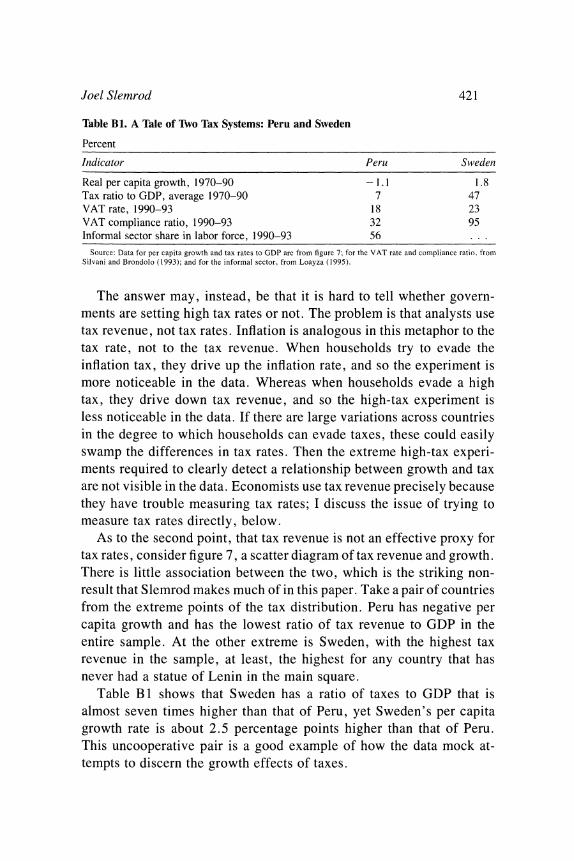
Joel Slemrod 421

Table BI. A Tale of Two Tax Systems: Peru and Sweden

Percent

Indicator Peru Sweden

Real per capita growth, 1970-90 - 1 .1 1 .8 Tax ratio to GDP, average 1970-90 7 47 VAT rate, 1990-93 18 23 VAT compliance ratio, 1990-93 32 95 Informal sector share in labor force, 1990-93 56 ...

Source: Data for per capita growth and tax rates to GDP are from figure 7; for the VAT rate and compliance ratio, from Silvani and Brondolo (1993); and for the informal sector, from Loayza (1995).

The answer may, instead, be that it is hard to tell whether governments are setting high tax rates or not. The problem is that analysts use tax revenue, not tax rates. Inflation is analogous in this metaphor to the tax rate, not to the tax revenue. When households try to evade the inflation tax, they drive up the inflation rate, and so the experiment is more noticeable in the data. Whereas when households evade a high tax, they drive down tax revenue, and so the high-tax experiment is less noticeable in the data. If there are large variations across countries in the degree to which households can evade taxes, these could easily swamp the differences in tax rates. Then the extreme high-tax experiments required to clearly detect a relationship between growth and tax are not visible in the data. Economists use tax revenue precisely because they have trouble measuring tax rates; I discuss the issue of trying to measure tax rates directly, below.

As to the second point, that tax revenue is not an effective proxy for tax rates, consider figure 7, a scatter diagram of tax revenue and growth. There is little association between the two, which is the striking non- result that Slemrod makes much of in this paper. Take a pair of countries from the extreme points of the tax distribution. Peru has negative per capita growth and has the lowest ratio of tax revenue to GDP in the entire sample. At the other extreme is Sweden, with the highest tax revenue in the sample, at least, the highest for any country that has never had a statue of Lenin in the main square.

Table B 1 shows that Sweden has a ratio of taxes to GDP that is almost seven times higher than that of Peru, yet Sweden's per capita growth rate is about 2.5 percentage points higher than that of Peru. This uncooperative pair is a good example of how the data mock attempts to discern the growth effects of taxes.


The next step is to go behind tax revenue and look at tax rates in this pair of countries. One tax rate for which there are data across countries is the value added tax (VAT) rate. It is also possible to obtain data on VAT revenue across countries. Carlos Silvani and John Brondolo com- pute the ratio of actual VAT payments to legally required VAT payments-the tax compliance ratio-from data on statutory VAT tax rates, VAT revenue, and the legal tax base.3 They find large variations in compliance ratios across countries, which can be seen from table B 1 in the drastically lower compliance ratio in Peru than in Sweden.

It is really this difference in tax compliance that explains the difference between the ratio of tax revenue to GDP in Peru and in Sweden. The statutory VAT tax rate is less than one-third higher in Sweden than in Peru. This is not the dramatic experiment that might have been expected from the fact that Sweden has seven times the tax revenue of Peru. Other growth determinants in the two countries swamp any mod- est effects of the difference in tax rates.

In regard to the third point, the crucial reason why Peru's compliance is so different from Sweden's is that Peru has a large informal sector, as table B1 shows. There is no direct estimate of Sweden's informal sector, but it seems obvious that it is smaller than that of Peru at 56 percent of GDP. In Peru a firm has the opportunity to escape taxation by shifting production into the informal sector; in Sweden this opportunity is much less widely available. The tax rate influences the size of the informal sector, but its size also varies for other reasons, external to the analysis.

The existence of this exit opportunity has implications like those of the evasion technologies that Slemrod discusses for the U.S. tax code. The results could be similarly subtle. Suppose that there is no big loss of efficiency associated with shifting into the informal sector. Suppose, also, that there is not really any need for the tax revenue because the government is not going to put it to productive use anyway. In this case, the informal sector just allows citizens to protect themselves against the tax policies of the government. So there is not likely to be much tax effect at all, if there is an easily available informal sector.

On the other hand, it could be costly to substitute informal sector production for formal sector production. There could be a large effi-

3. See Silvani and Brondolo (1993).

Joel Slemrod 423

ciency loss from shifting production out of modern factories into back- yard workshops in order to hide from the tax authorities. If there are such losses, then there will be large tax effects on growth. These growth losses happen even though there is very little tax revenue at the end of the day.

The informal sector could provide a simple explanation for the in- verse relationship that Slemrod notes between measures of distortions (for example, financial repression) and tax revenue. If the government has distortionary policies, it drives even more production out of the formal sector. The government cannot raise much tax revenue if a large proportion of the production is hiding in the informal sector.

For these and other reasons, tax revenue does not work well as a proxy variable for the marginal tax rate. So the immediate solution would seem to be to obtain tax rate data. As a soldier in the army of researchers that has tried to storm the stronghold of international tax data, I cannot be too encouraging. This citadel has, so far, held out against the siege. It is very hard to figure out from the welter of international tax codes exactly what the statutory tax rate is in a given country. Nor it is it trivial to trace how statutory rates map into the effective marginal tax rate facing the average person. Moreover, crucial variables, such as tax penalties, enforcement, and corruption, are mostly unobservable.

This is not to say that all cross-country explorations of aggregate fiscal variables are impossible. Some things are more easily measured than others. Many researchers have detected an association between high budget deficits and low growth. Others have found a strong association between government investment in infrastructure and growth, even if causality remains unresolved. There is a robust reduced-form relationship between size of government and such country characteris- tics as per capita income, population size, and share of agriculture. Further work on this relationship could be a useful check on the kinds of demand-for-government models that Slemrod discusses.4

However, I believe that most of the information about government intervention in markets will not come from aggregate fiscal variables. Instead, it will come from the more indirect measures of government

4. See Easterly and Rebelo (1993) for references and discussion of some of the relevant associations.


intervention in the economy, such as inflation rates, price distortions, black market premiums, and financial repression. The more extreme of these interventions, at least, are associated with low economic growth. Evidence has so far been insufficient to convict government on the charge of lowering growth through formal taxation. On other tax-like interventions, government is likely to be found guilty as charged.

General Discussion

Members of the panel suggested a variety of potential theoretical and empirical explanations for the weak relationship in the cross-country data between the size of government and growth. Christopher Sims noted that Bagwell and Bernheim's paper on Ricardian equivalence provides one explanation, since government activities may substitute for those that would otherwise be carried out by private institutions. For example, in less developed economies, private activities include social insurance, and a variety of village-level organizations perform some of the functions of a welfare state. Whether the costs and benefits of such functions are associated with the central government or the private sector thus depends on the particular institutional arrangements that have evolved.

Benjamin Friedman noted the relevance of this argument to the cur- rent political debate. He observed that assistance provided through churches, foundation charities, and family networks that, according to today's conservatives, is to take the place of many government activities is subject to the same tension between equity and incentives as that created when government provides assistance. Hence he suggested that the two arguments made by conservatives, that government welfare will be replaced by private welfare, and that this reduction in government involvement in social insurance will enhance the incentives for growth, are inconsistent. According to Friedman, it is likely that incentives will be enhanced only to the extent that replacement of government assistance is incomplete. James Duesenberry asserted that there is no need for a new experiment to determine whether private charity would re- place government social programs, pointing out that this country's experience in the nineteenth century makes it clear that private charity will not suffice in an industrial society.

Joel Slemrod 425

Richard Cooper argued that looking for evidence of a relationship between government size and growth in cross-country data is misguided. Even if such a relationship were to be found, he argued that it would not imply a causal link between government size and growth, and he gave two examples to underline this point. First, assuming that government expenditures are largely services provided by labor, as countries become wealthy wages rise relative to the prices of goods so that the ratio of G to Y rises, even with constant real expenditures on government services. As a result, in a cross-country regression there will be a positive relationship between growth and the G-to-Y ratio, even though there is no causal relation between the two. Second, almost all communist countries grew rapidly in the 1950s and 1960s and also had large governments that were investing large surpluses extracted from the public. But neoclassical growth theory teaches that economies that save a lot and start with low capital stocks will experience strong growth before decreasing returns eventually reduce the growth incre- ment to zero. The lesson is that government size, per se, is not informative; analysis needs to focus more precisely on the mechanisms by which government may affect growth.

Henry Aaron suggested another pitfall in using size to judge the impact of the public sector on economic growth. Variations in the size of the public sector arise from whether the government assumes direct or indirect responsibility for social programs. One country might rely on an extensive government social insurance program, and another might achieve the same social objective by regulating private pension plans. Alternative approaches would lead to large differences in the size of the measured public sector, even though the effects on growth would be similar. He asked whether anyone thought that there was a first-order difference in the distortion associated with financing a given amount of health care through payroll taxes, rather than through the private sector in a substantially involuntary way. According to Aaron, if the United States had the financing structure of Britain, France, or Germany it would have a public sector larger by 5 or 6 percentage points of GDP without significantly changing the government's direct or indirect effect on the economy.

James Poterba cautioned that the weak relationship between government size and growth in the data should not be taken as evidence that taxes have no effect on economic activity. In particular, this weak


relationship should not be seen as evidence for disregarding distortive effects of high marginal tax rates or inefficient public expenditures. Poterba was, nonetheless, puzzled by the weak results, since he had expected that the correlation between distortionary marginal tax rates and measures of the size of government would be quite strong However Cooper noted that, from his knowledge of individual countries, he would not expect a high correlation across countries of marginal tax rates with the ratio of tax revenue to GNP.

Panel members also suggested alternatives to the cross-country approach followed in this paper. Sims noted that several recent real business cycle models include an explicit government sector. These models treat taxes and government spending separately, and so are able to address the central question of what happens to growth when the effects of distortionary taxation and productive spending are considered si- multaneously. Although the calibration of such models does not lead to precise answers, the framework allows exploration of this combined effect under a variety of assumptions about how taxes and expenditures each affect the production process. Sims also pointed out that cross- section studies of U.S. states appear to find potentially positive effects of government spending on growth. Although these studies suffer from some of the same identification problems that beset cross-country studies, they are less vulnerable to the charge that substantial cultural and institutional differences across countries contaminate the results.

John Shoven commented on the treatment of government in com- putational general equilibrium (CGE) models. CGE analysis is predom- inantly used for differential tax analysis, looking at how different tax regimes can finance the same total revenue and the same government expenditure package. While these studies provide information about the marginal excess burden of various taxes, they are necessarily silent on the issue of small versus large government. Shoven noted that better understanding of the way government expenditures directly affect private productivity is a prerequisite for using the CGE framework. Even marginal excess burden calculations are based on tenuous assumptions; such calculations require marginal tax rates, but neither statutory rates nor information on tax shares provides a satisfactory measure of the marginal rates facing a typical agent.

Several panel members commented on the relevance of the Swedish experience to the debate over small versus large government. Robert

Joel Slemrod 427

Hall argued that Sweden's economic success with a large public sector may reflect the fact that the government has successfully suppressed value-destroying activities, like organized crime. A large G-to-Y ratio may not have a negative impact on growth because effective government may be highly correlated with the size of the government sector. In support of this hypothesis, Hall cited the success of large corporations that effectively function, internally, as command economies, much like the government sector in Sweden. In part, large corporations are successful because they, too, suppress value-destroying activities. Gregory Mankiw thought the large corporation analogy a useful one, since an employee who does not perform a specific task is fired. This is analogous to the Swedish approach to unemployment, whereby the unemployed are found jobs by the government and their benefits are terminated if they do not accept these employment opportunities. Hall added that through most of the postwar period, in both Sweden and Israel, work was effectively compulsory. Someone who did not accept the counseling of the employment service about what job to take was dropped from the system and punished severely. In this sense, Hall thought that the Swedish and the Israeli cases resemble the extended family.

John Haltiwanger noted that advocates of small government cite allocative inefficiencies arising from the distortions created by the tax structure or regulation. Seemingly inconsistent with this view, Sweden has among the highest rates of job creation and job destruction in the OECD. Even with what is regarded as a nonmarket and heavy-handed approach, Sweden seems to be reallocating jobs across production sites at a rapid rate. Duesenberry noted that Sweden has a very active labor reallocation system that has the cooperation of both workers and employers. The similarity of Scandinavian countries in terms of government size and growth record led Robert Shiller to raise the possibility that cultural differences, rather than differences in government size, might account for differences in growth rates across countries. He proposed a spatial autoregressive model where the growth rate would be regressed on the neighbors' incomes and government variables to see if government size still significantly affected growth.


References

Agell, Jonas, Thomas Lindh, and Henry Ohlsson. 1995. "Growth and the Public Sector: A Critical Review Essay." Unpublished paper. Uppsala Uni- versity (May).

Arcand, Jean-Louis, and Marcel Dagenais. 1994. "Economic Growth in a Cross Section of Countries: Do Errors in Variables Really Not Matter?" Unpublished paper. University of Montreal (May).

Atkinson, A. B. 1995. "The Welfare State and Economic Performance." National Tax Journal 48(2): 171-98.

Barro, Robert J. 1990. "Government Spending in a Simple Model of Endog- enous Growth." Journal of Political Economy 98(5, part 2): S 103-25.

. 1991a. "A Cross-Country Study of Growth, Saving, and Govern- ment." In National Saving and Economic Performance, edited by B. Doug- las Bernheim and John B. Shoven. Chicago: University of Chicago Press.

. 1991b. "Economic Growth in a Cross Section of Countries." Quar- terly Journal of Economics 106(2): 407-43.

. 1995. "Inflation and Economic Growth." Bank of England Quarterly Bulletin 35(2): 166-76.

Barro, Robert J., and Xavier Sala-i-Martin. 1992. "Public Finance in Models of Economic Growth." Review of Econiomic Studies 59(4): 645-61.

Baumol, William J. 1967. "Macroeconomics of Unbalanced Growth: The Anatomy of Urban Crisis." American Economic Review 57(3): 415-26.

Bergstrom, Theodore C., and Robert P. Goodman. 1973. "Private Demands for Public Goods." American Economic Review 63(3): 280-96.

Blumenthal, Marsha, and Joel Slemrod. 1992. "The Compliance Cost of the U.S. Individual Income Tax System: A Second Look After Tax Reform." National Tax Journal 45(2): 185-202.

Bolnick, Bruce R. 1978. "Demographic Effects on Tax Ratios in Developing Countries. " Journal of Development Economics 5(3): 283-306.

Bruno, Michael, and William Easterly. 1995. "Inflation Crises and Long-Run Growth." Working Paper 5209. Cambridge, Mass.: National Bureau of Economic Research (August).

Buchanan, James M., and Richard E. Wagner. 1977. Democracy in Deficit: The Political Legacy of Lord Keynes. New York: Academic Press.

Calmfors, Lars, and John Driffill. 1988. "Bargaining Structure, Corporatism, and Macroeconomic Performance." Economic Policy 6: 13-61.

Cameron, David R. 1978. "The Expansion of the Public Economy: A Com- parative Analysis." American Political Science Review 72(4): 1243-61.

Carr, Jack L. 1989. "Government Size and Economic Growth: A New Frame- work and Some Evidence from Cross-Section and Time-Series Data: Com- ment." American Economic Review 79(1): 267-71.

Joel Slemrod 429

Clotfelter, Charles T. 1995. "Public Services versus Private Philanthropy: Are There Winners and Losers?" Unpublished paper. Duke University (July).

De Gregorio, Jose. 1993. "Inflation, Taxation, and Long-Run Growth." Jour- nal of Monetary Economics 31(3): 271-98.

Drazen, Allan, and Vittorio Grilli. 1993. "The Benefit of Crises for Economic Reforms." American Economic Review 83(3): 598-607.

Easterly, William. 1993. "How Much Do Distortions Affect Growth?" Jour- nal of Monetaty Economics 32(2): 187-212.

Easterly, William, and Sergio Rebelo. 1993. "Fiscal Policy and Economic Growth: An Empirical Investigation." Journal of Monetary Economics 32(3): 417-58.

Engen, Eric, and Jonathan Skinner. 1992. "Fiscal Policy and Economic Growth." Working Paper 4223. Cambridge, Mass.: National Bureau of Economic Research (December).

Feldstein, Martin. 1995. "College Scholarship Rules and Private Saving." American Economic Review 85(3): 552-66.

Feldstein, Martin, and Andrew Samwick. 1992. "Social Security Rules and Marginal Tax Rates." National Tax Journal 45(1): 1-22.

Fischer, Stanley. 1993. "The Role of Macroeconomic Factors in Growth," Journal of Monetary Economics 32(3): 485-512.

Freeman, Richard B. 1995. "The Large Welfare State as a System." American Economic Review, Papers and Proceedings 85(2): 16-21.

Goode, Richard. 1968. "The Tax Burden in the United States and Other Countries. " Annals of the American Academy of Political and Social Science 379: 83-89.

International Monetary Fund. 1994. Government Finance Statistics Yearbook. Washington: International Monetary Fund.

Johnston, T. L. 1962. Collective Bargaining in Sweden. Cambridge, Mass.: Harvard University Press.

Kerr, Clark, and others. 1960. Industrialism and Industrial Man. Cambridge, Mass.: Harvard University Press.

King, Robert G., and Sergio Rebelo. 1990. "Public Policy and Economic Growth: Developing Neoclassical Implications." Journal of Political Econ- omy 98(5, part 2): SI126-50.

Levine, Ross, and David Renelt. 1991. "Cross-Country Studies of Growth and Policy: Methodological, Conceptual, and Statistical Problems." PRE Work- ing Paper 608. Washington: World Bank (March).

1992. "A Sensitivity Analysis of Cross-Country Growth Regres- sions." American Economic Review 82(4): 942-63.

Lindbeck, Assar. 1975. "Business Cycles, Politics and International Economic Dependence." Skandinaviska Enskilda Banken Quarterly Review 2: 53-68,


. 1995. "Hazardous Welfare-State Dynamics." American Economic Review, Papers and Proceedings 85(2): 9-15.

Loayza, Norman V. 1995. "The Economics of the Informal Sector: A Simple Model and Some Empirical Evidence from Latin America." Unpublished paper. World Bank (October).

Lucas, Robert E., Jr. 1988. "On the Mechanics of Economic Development." Journal of Monetary Economics 22(1): 3-42.

Marsden, Keith. 1983. "Links between Taxes and Economic Growth: Some Empirical Evidence." Working Paper 605. Washington: World Bank.

Messere, K. C. 1993. Tax Policy in OECD Countries: Choices and Conflicts. Amsterdam: IBFD Publications BV.

Musgrave, Richard A. 1969. Fiscal Systems. New Haven, Conn.: Yale Uni- versity Press.

Myrdal, Gunnar. 1960. Beyond the Welfare State: Economic Planning and Its International Implications. New Haven, Conn.: Yale University Press.

Niskanen, William A., Jr. 1971. Bureaucracy and Representative Government. Chicago: Aldine Atherton.

Organisation for Economic Co-operation and Development. 1994. Revenue Statistics of OECD Member Countries: A Standardized Classification. Paris: Organisation for Economic Co-operation and Development.

Peacock, Alan T., and Jack Wiseman. 1961. The Growth of Public Expenditure in the United Kingdom. Princeton, N.J.: Princeton University Press.

Peltzman, Sam. 1980. "The Growth of Government." Journal of Law and Economics 23(2): 209-87.

Plosser, Charles I. 1992. "The Search for Growth." In Policies for Long-Run Economic Growth. Kansas City, Mo.: Federal Reserve Bank of Kansas City.

Rebelo, Sergio. 1991. "Long-Run Policy Analysis and Long-Run Growth." Journal of Political Economy 99(3): 500-21.

Romer, Paul M. 1990. "Capital, Labor, and Productivity." BPEA, Microeco- nomics, 1990, 337-67.

Sachs, Jeffrey D., and Andrew Warner. 1995. "Economic Reform and the Process of Global Integration." BPEA, 1:1995, 1-95.

Silvani, Carlos, and John Brondolo. 1993. "An Analysis of VAT Compli- ance." Unpublished paper. International Monetary Fund (November).

Slemrod, Joel. 1992. "Do Taxes Matter?: Lessons from the 1980s." American Economic Review, Papers and Proceedings 82(2): 250-56.

. 1994. "A General Model of the Behavioral Response to Taxation." Unpublished paper. University of Michigan (September).

Slemrod, Joel, and others. 1994. "The Optimal Two-Bracket Linear Income Tax." Journal of Public Economics 53(2): 269-90.

Joel Slemrod 431

Solow, Robert M. 1956. "A Contribution to the Theory of Economic Growth." Quarterly Journal of Economics 70(1): 65-94.

Steinmo, Sven. 1993. Taxation and Democracy: Swedish, British and Ameri- can Approaches to Financing the Modern State. New Haven, Conn.: Yale University Press.

Summers, Lawrence H., Jonathan Gruber, and Rodrigo Vergara. 1993. "Tax- ation and the Structure of Labor Markets: The Case of Corporatism." Quar- terly Journal of Economics 108(2): 385-41 1.

Summers, Robert, and Alan Heston. 1991. "The Penn World Table (Mark 5): An Expanded Set of International Comparisons, 1950-1988." Quarterly Journal of Economics 106(2): 327-68.

Tanzi, Vito. 1992. "Structural Factors and Tax Revenue in Developing Coun- tries: A Decade of Evidence." In Open Economies: Structural Adjustment and Agriculture, edited by Ian Goldin and L. Alan Winters. Cambridge: Cambridge University Press.

U.S. Bureau of the Census. 1975. Historical Statistics of the United States, Colonial Times to 1970. Washington: Department of Commerce.

Wagner, Adolph. 1883. "The Nature of the Fiscal Economy," translated by Nancy Cooke. In Classics in the Theory of Public Finance, edited by Richard A. Musgrave and Alan T. Peacock. New York: Macmillan, 1958.

what do cross-country studies teach about … · teach about government involvement, prosperity,...

Documents