what drives rural youth welfare? the role of spatial

IFAD RESEARCHSERIES

42

What drives rural youth welfare?The role of spatial, economic, and household factors

byAslihan ArslanDavid TschirleyEva-Maria Egger

Papers of the 2019 Rural Development Report

The opinions expressed in this publication are those of the authors and do not necessarily represent

those of the International Fund for Agricultural Development (IFAD). The designations employed and the

presentation of material in this publication do not imply the expression of any opinion whatsoever on

the part of IFAD concerning the legal status of any country, territory, city or area or of its authorities, or

concerning the delimitation of its frontiers or boundaries. The designations “developed” and “developing”

countries are intended for statistical convenience and do not necessarily express a judgement about the

stage reached in the development process by a particular country or area.

This publication or any part thereof may be reproduced for non-commercial purposes without prior

permission from IFAD, provided that the publication or extract therefrom reproduced is attributed to IFAD

and the title of this publication is stated in any publication and that a copy thereof is sent to IFAD.

Authors:

Aslihan Arslan, David Tschirley, Eva-Maria Egger

© IFAD 2019

All rights reserved

ISBN 978-92-9072-959-4

Printed December 2019

The IFAD Research Series has been initiated by the Strategy and Knowledge Department in order to bring

together cutting-edge thinking and research on smallholder agriculture, rural development and related

themes. As a global organization with an exclusive mandate to promote rural smallholder development,

IFAD seeks to present diverse viewpoints from across the development arena in order to stimulate

knowledge exchange, innovation, and commitment to investing in rural people.

IFAD RESEARCHSERIES

42

byAslihan ArslanDavid TschirleyEva-Maria Egger

What drives rural youth welfare? The role of spatial, economic, and household factors

This paper was originally commissioned as a background paper for the 2019 Rural Development Report: Creating opportunities for rural youth.

www.ifad.org/ruraldevelopmentreport

Acknowledgements

Funding for this research was provided by IFAD. The authors are thankful to all the

participants of the Rural Development Report (RDR) workshops held throughout the

content development phase. Special thanks to Paul Winters for leading and contributing

to the analytical content of the RDR, based on which the research ideas for this paper

were developed. The authors also thank to Margherita Squarcina, Michael Dolislager

and Fabian Löw for excellent research assistance. This background paper was prepared

for the Rural Development Report 2019 “Creating Opportunities for Rural Youth”. Its

publication in its original draft form is intended to stimulate broader discussion around

the topics treated in the report itself. The views and opinions expressed in this paper are

those of the author(s) and should not be attributed to IFAD, its Member States or their

representatives to its Executive Board. IFAD does not guarantee the accuracy of the

data included in this work. For further information, please contact

[email protected]. IFAD would like to acknowledge the generous financial

support provided by the Governments of Italy and Germany for the development of the

background papers of the 2019 Rural Development Report.

About the authors

Aslihan Arslan is a senior research economist at the Research and Impact

Assessment Division of IFAD. She leads multiple research projects related to

agricultural productivity, climate resilience, rural migration and the climate change

mitigation potential of agricultural practices promoted by IFAD and others. She also

leads some impact assessments of IFAD projects related to these themes, and co-

leads the 2019 Rural Development Report on Creating Opportunities for Rural Youth.

Prior to joining IFAD in 2017, Aslihan worked as a natural resource economist for FAO,

focusing primarily on climate-smart agriculture. She holds a PhD and an MSc in

agricultural and resource economics from the University of California at Davis.

David Tschirley is fixed-term professor of international development in the Department

of Food, Agricultural, and Resource Economics at Michigan State University (MSU), and

co-director of the department’s Food Security Group. He is also a member of the Core

Technical Team of MSU’s Global Center for Food Systems Innovation. He has over 20

years of experience in applied food security research, mentoring of developing country

researchers and active policy outreach. He was the external lead author of the 2019 RDR

on creating opportunities for rural youth. He holds an MSc and a PhD in agricultural, food

and resource economics from MSU.

Eva-Maria Egger is an applied economist in the Research and Impact Assessment

Division of IFAD. She researches migration, climate change and rural development. She

also contributes to impact assessments of IFAD projects and the 2019 RDR on creating

opportunities for rural youth. Before joining IFAD, Eva-Maria worked for the Migrating out

of Poverty Research Consortium funded by the UK Department for International

Development (DFID). She holds a PhD and an MSc in economics from the University of

Sussex, UK, and a BA in political science and economics from the Albert-Ludwigs-

University in Freiburg, Germany.

Table of contents

1. Introduction 1

2. Conceptual framework: the rural opportunity space 2

3.1 Data and variables for global analysis of the rural opportunity space 4

3.2 Merging global data with household-level data 6

3.3 Methodology to assess welfare of rural young households 9

4. Results 10

4.1 Where do rural youth live? 10

4.2 How do younger households fare and how does this depend on where they live? 15

4.3 Exploring potential correlates of welfare outcomes 18

5. Conclusion 23

References 24

Appendix A 27

Abstract

Most of the discourse on rural youth in developing countries lacks robust evidence on where ruralyouth live and how the challenges and opportunities of their location affect their welfareoutcomes. This paper uses the concept of the Rural Opportunity Space from economicgeography literature to shed light on these questions. Rural opportunities are expected to beshaped by commercial and agricultural potential of a location. We apply this conceptualframework to global geo-spatial data from 85 low- and middle-income countries on populationdensity, as a proxy for commercial potential, and a measure of greenness, as a proxy foragricultural potential, to locate rural youth within the opportunity space globally. We then combinethese data with household-level data from 12 countries in Africa, Latin America and Asia, toassess how the Rural Opportunity Space influences welfare outcomes of young householdscompared with older households. Our findings show that most rural youth actually live in areaswith high potential in terms of commercial and agricultural opportunities. However, their welfareoutcomes depend much more strongly on commercial potential than on agricultural potential.Education can have large poverty-reducing effects for younger households, especially in areaswhere commercialization potential is neither lowest nor highest.

Understanding the welfare outcomes of rural youththrough the "rural opportunity space":

Evidence from 12 developing countries around the world

1

1. IntroductionYouth have become an especially important issue in the international development discourserecently for several reasons. First, and most important, is the particular demographic transitionstage most developing countries find themselves in: youth constitute a high proportion of thepopulation – currently about one in five – in low-income countries. This compares with only one ineight in high-income countries. Furthermore, the absolute number of youth in Africa is risingrapidly, even as it has plateaued and begun to fall in the rest of the developing world 1

(UNDESA, 2017). High proportions of youth in the population and, in Africa, rapidly risingnumbers of youth pose major challenges for low-income countries needing to invest to improvetheir citizens’ future. Rural youth specifically constitute a high proportion of many developingcountries’ population (Stecklov and Menashe-Oren, 2019), while rural areas continue to lagbehind in economic development (Ghani, 2010).

Second, although the two biggest youth populations are in China, an upper-middle-incomecountry, and India, a lower-middle-income country, the majority of countries with large rural youthpopulations are low-income countries with high poverty rates and low levels of structuraltransformation. Most of these countries are in sub-Saharan Africa and Asia, where the highproportions of rural youth, large absolute numbers and widespread poverty make it verychallenging for them to invest to improve their citizens’ future. Poverty reduction and ruraldevelopment thus cannot be addressed without rural transformation being inclusive of rural youth(IFAD, 2016).

How to ensure this has been increasingly capturing the attention of development practitioners,policymakers and academics. Most of this discourse, however, lacks robust evidence on whererural youth live and how these spaces affect their welfare outcomes. This paper explores theoverlapping national, local and familial settings in which rural youth live. The intersection of thesesettings – the level of transformation of their national economy, the potential productivity andconnectivity of the particular area they live in, and the capacities of their families – determine ingreat part the opportunities available to rural youth. Conceptualizing rural youth challenges andopportunities in this way allows us to address three questions: (1) Where do rural youth live in thedeveloping world in terms of agricultural and commercial potential? (2) How do these varyingagricultural and commercial potentials affect the welfare outcomes of younger households withina country? (3) Does the hypothesized disadvantage of younger households compared with olderhouseholds vary by transformation level?

This paper provides a conceptual framework to answer these questions using a spatial typologyand applies it at global and household levels. To this end, we use spatially explicit populationdensity data from the WorldPop project and the Moderate Resolution Imaging SpectroradiometerEnhanced Vegetation Index (MODIS EVI), to define, respectively, commercialization andagricultural potentials that make up the axes of the rural opportunity space. At the householdlevel, we combine spatial data with 12 nationally representative datasets that span Africa, LatinAmerica and Asia to define welfare indicators, and variables posited to affect them. Our spatialtypology builds a “rural opportunity space” (ROS) drawing on the concept of “landscapes ofopportunity” by placing rural youth on a rural-urban gradient that represents commercializationpotential and a gradient representing agricultural potential (Ripoll et al., 2017; Abay et al., 2019).We posit that, controlling for the level of structural transformation that a country has achieved,_______________________________1 We use “developing world” to refer to low- and middle-income countries, as defined by the World Bank (2018a).We use “developing world” and “low- and middle-income countries” interchangeably to refer to the same set ofcountries.

Understanding the welfare outcomes of rural youththrough the "rural opportunity space":Evidence from 12 developing countries around the world

2

these factors substantially shape the range and attractiveness of opportunities available to ruralyouth. Whether or not rural youth can capitalize on opportunities presented by their geographicalspace and their country’s economic structure, however, is subject to multiple constraints andclosely linked to the characteristics of the households in which they live. Therefore, wedifferentiate between younger and older households. After careful documentation of rural youthwithin the spatial typology, we analyse welfare outcomes and how these change by typology todraw policy implications. Using our global definition of the rural-urban gradient instead ofinconsistent administrative definitions of urban areas, we find that more than three quarters of thedeveloping world’s rural (non-urban) youth live in the areas with most agricultural potential, whileonly 7 per cent are found in areas with the lowest potential. Our analysis of welfare outcomesreveals that households with mostly young members are more likely to be poor than mostly olderhouseholds, in all types of countries independent of the level of transformation. In terms of theROS, commercialization potential relates strongly to poverty reduction whereas agriculturalpotential per se does not. The young household penalty is worst in the subsample of leasttransformed countries, and seems smallest in the most transformed countries in our analysis. Theschooling bonus in terms of welfare outcomes is highest in less densely populated areas and inthe least transformed economies. These findings underline the importance of addressingconnectivity challenges to improve the opportunities for the majority of rural youth.

2. Conceptual framework: the rural opportunity spaceThis paper assesses how the characteristics of the location where rural youth live shape theirlivelihoods. Yet neither the national structure of an economy nor the household structure in whichyouth live can be ignored. A more productive economy will increase the payoff to investmentsspecific to rural youth. Sustained growth and structural transformation are typically associatedwith public commitment to investments in education, health and infrastructure (World Bank,2018b). As a consequence, in countries that make these investments, more educated and skilledyouth have more opportunities and agency to employ their skills productively.

Within a country, rural youth opportunities vary by location. While an economy may beexperiencing structural transformation at the national level, not all areas within the country will betransforming equally. In rural areas, opportunities are determined to a large extent by access tomarkets (for agricultural output, inputs, labour, finance and others) that determines the area’scommercialization potential, and by the natural resource base that determines the agriculturalpotential of the area. Both of these factors have strong spatial dimensions (Wiggins and Proctor,2001; Ripoll et al., 2017). Together, these two factors form the ROS (figure 1) that affects theopportunities and challenges rural youth face, subject to the characteristics of the broadernational economy as well as individual- and household-level constraints. This economicgeography framework structures what is possible at the highest level within a given country,independent of local context, specific social norms or any individual preferences (Abay et al.,2019).



3

Figure 1. Rural opportunity space

Source: Authors’ conceptualization

Commercialization potential increases with connectivity to cities, their markets and potential forprivate-sector investment, all of which are crucial for extending opportunities to rural youth.Promisingly, secondary cities closer to rural areas are growing faster than more distant capitalcities (Roberts and Hohmann, 2014). This expansion of secondary cities and towns hasgenerated more poverty reduction than has the growth of large metropolitan areas, among otherreasons by providing more accessible migration targets for rural residents (Tanzania, forexample; Christiaensen et al., 2013) and by displaying more inclusive growth patterns (India;Gibson et al., 2017). Yet physical and virtual connections of these urban centres with rural areasare often poor. Many needed connections depend on public goods, such as improved roads andcommunications infrastructure, but also on private investment. Increasingly, the private sector isproviding mobile technology, post-harvest facilities and processing, and agricultural inputs in ruralareas. Public goods such as improved roads and well-designed legal and regulatory systems arenecessary for private investments to take place on a broad scale, however. The vast majority ofrural youth in developing countries live as dependants within larger families (Doss et al., 2019).Thus, in addition to the ROS in which youth reside, the characteristics of the household in whichyouth live also influence the set of opportunities and challenges that youth face. As youthtransition from adolescence to adulthood, they begin to form their own households or stay longerwith their parents. The two trajectories are associated with different challenges and opportunities.We therefore distinguish households by their demographic composition and define mostlyyounger and mostly older households. Mostly younger households include those with manydependent youth as well as newly formed young households, which usually lack experience andassets that take time to accumulate. Youth in mostly older households are expected to benefitfrom assets and experiences of their parents leading to better welfare outcomes (holding all else


4

constant). In the next section, we present the details of spatial data used to operationalize theROS and nationally representative survey data to analyse how the ROS affects welfare of ruralhouseholds and their youth.

3. Data and methods

3.1 Data and variables for global analysis of the rural opportunity space

To create a typology of the ROS, we use commercialization potential and agricultural productionpotential as two axes of the opportunity space. Commercialization potential is proxied by populationdensity data from the WorldPop project, and agricultural potential is proxied by the EnhancedVegetation Index (EVI), which stems from satellite observations.

Commercialization potential

Administrative definitions of “rural” and “urban” suffer from two analytical problems. First, they differacross countries, which reduces the usefulness of cross-country comparisons. Second, the definitionsare based on a simple dichotomy that may be increasingly at odds with how people actually live.Urban and rural qualities have become increasingly blurred by rapid urbanization, increased ruralpopulation densities and economic transformation in rural areas that has driven an increase in “urban”characteristics such as reliance on markets. The increasing prevalence and growth of small andsecondary towns plays an important role in connecting the two geographical dimensions andcatalysing commercialization opportunities (Lerner and Eakin, 2010). Moreover, the transformation ofagri-food systems (AFS) has increased the economic linkages between rural areas and cities(Dolislager et al., 2019), increasing the need for a more fluid spatial definition. One approach toreconciling this is through the increasing application of the concept of “peri-urban areas” (Simon et al.,2006; Simon, 2008). These areas can be seen as rural locations that have “become more urban incharacter” (Webster, 2002, page 5); and as sites where households pursue a wider range of income-generating activities while still residing in what appear to be areas of rural character (Lerner and Eakin,2010).

Commercialization potential can be measured by road density, average time to nearest market orpopulation density, each with its own challenges (Abay et al., 2019). Instead of applying administrativerural and urban definitions, we therefore use high-resolution population densities from the WorldPopproject to create a rural-urban gradient (see Jones et al., 2016, for a recent application). Spatiallyexplicit global population density data are used to proxy commercialization potential, with the idea thatit correlates with agricultural commercialization, off-farm diversification and market density (Bilsborrow,1987; Wood, 1974). This approach ensures comparability across regions and countries and creates amore precise spatial picture, which allows a better understanding of economic and socialcharacteristics of individuals and households over space. The WorldPop project provides250 m × 250 m resolution population density maps for each country in the world. The production of theWorldPop datasets principally follows the methodologies outlined by Tatem et al. (2007),Gaughan et al. (2013), Alegana et al. (2015) and Stevens et al. (2015). WorldPop also includesage-and gender-differentiated spatially explicit information on population distributions (at 1 kmresolution), which we use to locate rural youth around the developing world. We include 85 low- andmiddle-income countries2 from the global database, for which we have complete data. To define aglobally comparable scale of the rural-urban gradient, all grids were ordered from least to most dense,_______________________________2 As defined by the World Bank (2018a).



5

and population was successively summed to create four quartiles of equal population, ranging fromleast to most densely settled areas. The least dense quartile represents rural hinterland areas, whilethe most dense quartile represents the urban areas. In between are semirural (second quartile) andperi-urban (third quartile) areas.3 Table 1 displays how our categorization into four groups compareswith the administrative rates of urbanization by region. In all regions, official urbanization rates fromadministrative sources are higher than those in our population-density-based definition. The differenceis, however, starkest in Latin America and the Caribbean (LAC) and in countries in the Near East,North Africa, Europe and Central Asia (NEN). In sub-Saharan Africa (SSA) and Asia and the Pacific(APR), although the difference is smaller, the administrative urbanization rate is very similar to theurban and peri-urban areas of the rural-urban gradient combined.

Table 1. Comparing the population shares within the categories of the population density based rural-urbangradient to urbanization rates from administrative sources by region

Regions

Population density based rural-urban gradient AdministrativeurbanizationrateRural Semirural Peri-urban Urban

LAC 41.84 16.03 20.33 21.80 67.30

SSA 46.75 13.58 14.43 25.24 38.03

APR 33.31 23.24 23.82 19.63 38.04

NEN 43.32 12.91 18.32 25.45 56.75

Globalaverage 42.59 15.83 18.04 23.55 46.50

Notes: Population densities are from the WorldPop project, and administrative urbanization rates come from theUnited Nations Population Division for 85 low- and middle-income countries.

Agricultural potential

Vegetation indices based on remote sensing data are increasingly used as a proxy for agroecologicalpotential to facilitate global comparisons (Jaafar and Ahmad, 2015; Chivasa et al., 2017). MODIS EVI,excluding built and forested areas, is used here to measure the influence of geography on the potentialfor productivity in farming (figure 1). Global EVI data covering all developing countries at 250 m ×250 m resolution were aggregated to the 1 km level to match the resolution of age-disaggregatedpopulation data. By focusing on land classified as cropland or pasture, the analysis spatially targetsagricultural land to proxy agricultural production potential. Finally, average EVI values for the three-year period between 2013 and 2015 were calculated to minimize the impacts of seasonality andannual agro-climatic variation. EVI grids for all non-urban land were ordered from lowest to highestEVI, and all area was summed to create three groups (terciles) of equal total land area representingthe low, medium and high agricultural potential categories on the horizontal axis.

Using the combination of the above data, the number and proportion of rural (non-urban) youth in eachof the ROS categories were calculated and are presented below. For illustrations of where youtharound the world live, we also draw on the population data and projections from the United NationsPopulation Division (UNDESA, 2017).

_______________________________3 Table A.5 in Appendix A shows the population density threshold to define each quartile and the averagepopulation density within each quartile.


6

3.2 Merging global data with household-level data

To assess the economic engagement and opportunities of rural youth within the ROS, we look atthree main groups of variables: sectoral and functional employment type, education status andwelfare outcomes. To map these within the ROS, we merge the global ROS data with those of 12household surveys from countries in Latin America, sub-Saharan Africa and Asia. Thesecountries are Bangladesh, Cambodia and Nepal in Asia, Mexico, Nicaragua and Peru in LatinAmerica, and Ethiopia, Malawi, Niger, Nigeria, Tanzania and Uganda in sub-Saharan Africa.4

Given the importance of a country’s structural transformation level in facilitating the channelsthough which youth livelihoods are shaped, we group these countries in three categories: high,medium and low level of transformation. We use data on the proportion of non-agricultural GDPfor all low- and middle-income countries to define these categories (IFAD, 2016). As a result,Peru and Mexico are in the group of high transformation; Nicaragua and Bangladesh are in themiddle group; and the African countries as well as Cambodia and Nepal form the group of lowstructural transformation (table 2).5

Table 2. Study countries by level of structural transformation and region

Region

Level of structural transformation

Low Medium High

Latin America Nicaragua Mexico, Peru

Asia Cambodia, Nepal Bangladesh

Sub-Saharan Africa Ethiopia, Malawi, Niger, Nigeria,Tanzania, Uganda

Using available geo-spatial information about enumeration areas (EAs) or other administrativesampling units, the ROS data were merged with the household survey data.6 Population densityof each EA was calculated and then classified into the population density quartiles using theglobal thresholds defined above. The EVI for each EA was also calculated for the 2013-2015period as described above. While there are differences between the administratively defined ruraland urban areas and our spatially defined rural-urban gradients , these are small in most surveysof LAC and SSA. In Asia, many administrative rural areas are defined as peri-urban in ourdefinition because of the high population density, especially in Bangladesh.7

Variables that measure welfare outcomes of rural youth

As mentioned above, most rural youth live in households as dependants, so they experience thechallenges and opportunities determined by their household’s welfare. We differentiatehouseholds based on their demographic structure to analyse youth welfare. Youth living in mostlyyounger households are expected either to have started their own households (with potential

_______________________________4 A detailed list of all datasets and source of geolocation is presented in Appendix A, table A.7.5 See appendix table A.1 for the thresholds of each tercile and the level of non-agricultural percentage of GDP foreach of the 12 study countries.6 See methodological appendix B for a detailed explanation of the merging procedure.7 Table A.6 in Appendix A compares the population shares within each category of the rural-urban gradient with theadministrative rural or urban category provided in each survey by region.



7

challenges that are associated with being young as mentioned above) or to contributesubstantially to the livelihood of this household. In contrast, youth in mostly older householdsmight still be living with their parents and enjoy the freedom to continue to go to school and bearless responsibility for providing the household income. Among all households with at least oneyoung member, mostly younger households are defined as those with a proportion ofeconomically active young members above the national average; and mostly older householdsare those for which this proportion is below the national average.8 A similar approach is used byAbay et al. (2019) to discuss youth opportunities. The main variables of interest to measure thewelfare of rural youth are household poverty status and per capita expenditure. Other variables ofinterest include education, gender of the household head, land ownership, access to credit andincome sources. All variables are constructed in the same manner across all datasets to ensurecomparability.

Education is an important determinant of employment and welfare outcomes at both the individualand household levels. The most comparable variable available in the survey data is whether anindividual has completed secondary schooling or not. At the household level, we use theproportion of working-age household members with secondary education as an indicator of thehousehold’s education level.

Further variables of interest are the land ownership and income sources of households. Wedefine a dummy for households owning any land and, if they do, we compute the size of landrelative to household size. We define two variables to capture household livelihood structures:their level of diversification out of agriculture, measured by the proportion of non-farm income intotal income, and their commercialization within agriculture, measured by the proportion of farmsales in total farm income. Farm income and total income are constructed based on the RuralIncome Generation Aggregates (RIGA) methodology (Carletto et al., 2008; Davis et al., 2017).9

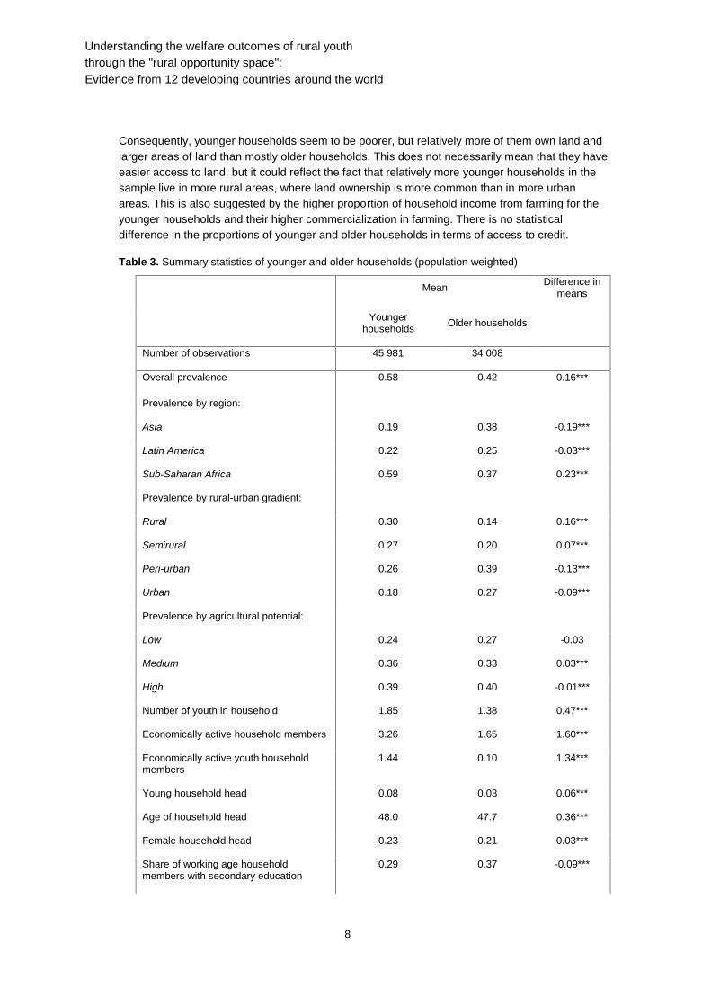
Table 3 shows the composition of younger and older households and their characteristics.10

Nearly 60 per cent of households are ‘mostly younger’, with the fewest young households in Asiaand the most in Africa. Younger households are evenly distributed along the rural-urban gradient,with slightly more living in rural hinterland than in urban areas. In contrast, relatively more olderhouseholds live in more densely populated areas. In terms of agricultural potential, similarproportions of younger and older households live in each category, most in areas with high ormedium potential. While younger and older households both have middle-aged household heads,younger households have on average more members who are youth and, on average, almost allyouth in a mostly younger household are economically active, while in mostly older householdsrelatively fewer of them are working. This difference is most striking and expected to shapewelfare outcomes differently, as is the smaller proportion of working-age household members withsecondary education in younger households. If youth have to contribute to the household'sincome generation, fewer of them can continue their education.

_______________________________8 We use the standard UN definition of youth as all individuals between 15 and 24 years old.9 All monetary values are expressed per capita over a daily basis in PPP (constant 2011 international dollars).Imputation techniques to treat outliers have been applied, replacing all the values above the ninety-ninth percentileof the distribution of each income component with the highest value within the ninety-ninth percentile, while for theaggregate income variables all the extreme values (above the ninety-ninth percentile and below the first percentile)have been replaced with missing values.10 Table A.8 in Appendix A presents the summary statistics of all characteristics for each country.


8

Consequently, younger households seem to be poorer, but relatively more of them own land andlarger areas of land than mostly older households. This does not necessarily mean that they haveeasier access to land, but it could reflect the fact that relatively more younger households in thesample live in more rural areas, where land ownership is more common than in more urbanareas. This is also suggested by the higher proportion of household income from farming for theyounger households and their higher commercialization in farming. There is no statisticaldifference in the proportions of younger and older households in terms of access to credit.

Table 3. Summary statistics of younger and older households (population weighted)

Mean Difference inmeans

Youngerhouseholds Older households

Number of observations 45 981 34 008

Overall prevalence 0.58 0.42 0.16***

Prevalence by region:

Asia 0.19 0.38 -0.19***

Latin America 0.22 0.25 -0.03***

Sub-Saharan Africa 0.59 0.37 0.23***

Prevalence by rural-urban gradient:

Rural 0.30 0.14 0.16***

Semirural 0.27 0.20 0.07***

Peri-urban 0.26 0.39 -0.13***

Urban 0.18 0.27 -0.09***

Prevalence by agricultural potential:

Low 0.24 0.27 -0.03

Medium 0.36 0.33 0.03***

High 0.39 0.40 -0.01***

Number of youth in household 1.85 1.38 0.47***

Economically active household members 3.26 1.65 1.60***

Economically active youth householdmembers

1.44 0.10 1.34***

Young household head 0.08 0.03 0.06***

Age of household head 48.0 47.7 0.36***

Female household head 0.23 0.21 0.03***

Share of working age householdmembers with secondary education

0.29 0.37 -0.09***



9

Mean Difference inmeans

Youngerhouseholds Older households

Poor (≤ $1.90 per capita per day in 2011international PPP dollars)

0.33 0.17 0.16***

Per capita expenditure (2011international PPP dollars)

3.51 4.65 -1.13***

Land ownership, dummy 0.57 0.36 0.21***

Land owned, in hectares 0.76 0.36 0.39***

Land per capita, in hectares 0.24 0.19 0.05***

Household has received any credit 0.25 0.25 -0.00

Farming share of total income 0.36 0.22 0.14***

Share of farm sales in own farm income 0.31 0.33 -0.03***

3.3 Methodology to assess welfare of rural young households

Where do rural youth live and how does this shape their welfare outcomes? The first part of thisquestion is assessed by combining various data sources to describe where rural youth live in the ROS.This is done first with global data and then with the household-level data. Then we use regressionanalysis to describe how the spatial variables that define the ROS as well as other characteristicsinfluence the welfare outcomes of rural young households and compare this with older households.The opportunities available to youth in their ROS affect their welfare outcomes through variouschannels including school-to-work transitions and economic engagement (IFAD, 2019; Dolislager etal., 2019). Notwithstanding the importance of understanding these various channels, we model welfareoutcomes using only the following equation:= + + + + + + ∗ + ∗ + ∗+ ∗ + + (1)

The welfare outcome of household h, , is measured by total expenditure or poverty and depends onthe agricultural potential, , and the commercialization potential, , of location j as defined above.

is the indicator variable for young households capturing the effects of the demographic structureon welfare outcomes. The proportion of adults with secondary education in the household ( ) isexpected to improve welfare outcomes. Households with female heads ( ) are expected tohave worse welfare outcomes than male-headed households. To assess how these variablesdifferentially influence welfare outcomes, each variable is interacted with the young householdindicator. is a series of country fixed effects, and is a normally distributed error term.

In all regressions, standard errors are clustered at the country level. For ease of comparingcoefficients, we compute marginal effects to present the results of interest and predicted probabilitiesfor graphical illustration. We also present results from various subsample regressions that follow thecorresponding methodology and specification.


10

4. Results

4.1 Where do rural youth live?

While the political discourse centres on African youth, most of the world's rural youth currently live inAsia, with the numbers of youth in China and India alone surpassing those of all sub-Saharancountries together (figure 2). Only in Asian countries are the numbers of semirural and peri-urbanyouth higher than those in rural hinterland areas. However, population projections indicate that sub-Saharan Africa is the only region where numbers of youth are expected to continue to increase so thatin 2050 the continent will hold the second largest share of all youth globally (UNDESA, 2017). In termsof level of transformation, countries with low levels of structural transformation have relatively moreyouth in rural hinterland areas than in semirural or peri-urban areas, pointing to the lack of connectivityyouth are exposed to in these economies. In contrast, countries with medium levels of transformationshow the opposite pattern. However, even the countries with relatively high levels of structuraltransformation in their economies have relatively more youth living in their rural than peri-urban areas.

The ROS presents a valuable framework to understand the opportunities and challenges the world’srural youth face at both the global and country levels to identify policy and investment opportunities fortheir inclusion in rural transformation. Figure 3 displays the distribution of all 778 million non-urbanyouth from 85 low- and middle-income countries within the ROS as defined in section 2. Two in threeof them live in areas with the highest agricultural potential. Only 7 per cent live in the lowest-potentialareas. This concentration of rural population, and thus of rural youth, in the most productive areas isnot surprising, as it reflects (especially in Africa) historical movement of agriculture-dependentpopulations to the most productive and least disease-prone areas of the world. This spatial patternsuggests that agricultural potential per se is not a primary constraining factor for a majority of ruralyouth. If their farming productivity is low, the reason most likely relates to lack of access to markets,both markets for inputs (e.g. improved seeds, fertilizer and credit) and markets for output to provideincentives to invest in increased productivity.



11

Figure 2. Non-urban youth populations in low- and middle-income countries in 2015 in millions, along therural-urban gradient: (a) by region; (b) by level of structural transformation.


12

Figure 3. Two out of every three rural youth in the developing world live in spaces with high agriculturalpotential

Note: Commercialization potential is defined using 2015 population density data for 85 low- and middle-incomecountries from the WorldPop project. All grids are ordered from least to most dense, and cut-offs are set to place 25per cent of population in each of four groups. The highest-density quartile is called urban. The remaining threequartiles each hold one third of the non-urban population and define the three groups of the rural-urban gradient:rural, semirural and peri-urban. These represent respectively the low, medium and high commercial potentialcategories on the vertical axis. Agricultural potential is defined using MODIS EVI for the same grids ordered fromlowest to highest. Each of the three groups (terciles) holds one third of all non-urban space and the represent thelow, medium and high agricultural potential categories on the horizontal axis.

The vast majority of global rural youth live in relatively densely settled areas. What is not shown in thefigure is that the least connected one third of the non-urban population (the bottom row of figure 3)occupy 92 per cent of non-urban land area, while the remaining two thirds live on the other 6 per centof non-urban land. This means that two thirds of the rural youth population live in areas that are onaverage 23 times more densely populated than the least connected one third. What this means is thatthe vast majority of non-urban land in the developing world is very sparsely populated, while the vastmajority of rural residents live in areas that are relatively densely populated. The potential forconnectivity – with markets, information, ideas and possibilities – is thus relatively high for many of thedeveloping world’s rural youth. If these youth are poorly connected and lack opportunities, the reasonsdo not relate to the potential productivity and connectivity of the land and spaces they occupy. Rather,they relate to the level of transformation in the broader economy in which they live (and thus thedensity of infrastructure and the size and dynamism of end markets), to the characteristics of thehouseholds in which they reside, and to constraints specific to youth and their individualcharacteristics.

The patterns identified above lend themselves to a classification of ROS in five groups that capture thebroad challenges and opportunities faced by developing countries’ rural youth. Around one quarter ofall rural youth in developing countries live in areas that combine the highest agricultural potential andthe highest potential connectivity (top-right cell in figure 3). These youth face diverse and potentially



13

remunerative opportunities, depending on the dynamism of the broader economy in which they reside.At the other extreme are the 4 per cent of rural youth who live in the least connected spaces with thelowest agricultural potential (bottom-left cell). They face severe challenges, again with the prospects ofovercoming them depending in large measure on the broader economy in which they reside and theparticular characteristics of the youth themselves and their families. Forty-three per cent of all ruralyouth live in spaces with high agricultural potential but limited access to markets, while those in spaceswith strong market access but lower agricultural potential represent only 9 per cent of the total. Theremaining one fifth of rural youth face an opportunity space with mixed challenges and opportunities.Since policy is made at the country level, we also highlight the county-level prevalence of the ROS forthe most extreme cases. A detailed picture of this can be found in the RDR (IFAD, 2019).11 Youthfacing the greatest challenges from their geography – those in “severe challenges” and “mixedchallenges” spaces – mostly live in Iran (22 per cent), followed by Brazil and China (around 10 percent each). All three have high levels of structural transformation, but appear to suffer from smallpockets of stubborn, persistent poverty, rather than widespread poverty. Ghani (2010) refers to this asthe lagging region problem. These countries should have the capacity to invest in these isolated ruralyouth, as they have more fiscal resources to do so than low-income countries.

Even though groups with severe and mixed challenges are least prevalent in the countries with lowestincome levels, 2 million youth in Afghanistan face severe challenges in their ROS – the largest countryprevalence in this group, at 36 per cent. Regionally, the mixed challenges group is most prevalent inAfrica: eight of the top 10 countries in terms of prevalence of youth with mixed challenges are in SSA.In the “diverse opportunities” space, six out of the 10 countries with the highest proportions of youthare in Asia. Nearly half of all rural youth – the largest group – enjoy high agricultural potential, but havelimited access to markets. This type of youth dominates African economies: seven of the top 10countries in this group are in Africa. Only 9 per cent of the developing world’s rural youth live in spaceswith strong market access but poor agricultural potential. Put another way, it is rare to see non-urbandense populations of people living in areas of low and medium productive potential. This pattern againreflects historical settlement of migrating populations in areas of high farming potential. Regionally,although the top three countries with highest prevalence are in the Near East and Central Asia, LatinAmerica has five of the top 10 countries. Most LAC countries are among the wealthiest in our group ofcountries with high urbanization rates, which could explain their dominance in this group with thehighest commercialization potential. Zooming in to household-level characteristics, we find that themajority of mostly younger households in our household sample is found in the mixed challenges andopportunities space (figure 4a).12 Comparing household location in the ROS within group oftransformation level does not reveal any difference between younger and older households (figure 4b).In our sample of 12 countries, households are relatively evenly distributed across the ROS categoriesof mixed challenges, high agricultural but low commercial potential, and high commercial but lowagricultural potential, in the high-transformation countries of Mexico and Peru. Bangladesh andNicaragua (medium structural transformation group) host most households in areas of high populationdensity but low agricultural potential, whereas in the countries with lowest levels of transformation(mostly in SSA) relatively more households live in areas of mixed or severe challenges than in othercountry groups. These findings underline the importance of a spatially explicit focus to policies andinvestments to improve youth inclusion in rural transformation.

_______________________________11 Table A.10 in Appendix A presents the data for each country from which the results are drawn.12 Table A.9 in Appendix A compares how rural youth in the sample of 12 countries are distributed across the ruralopportunity space with the distribution using global data about all low- and middle-income countries.


14

Figure 4. Prevalence of mostly younger and older households across the rural opportunity space categories:a) overall distribution by age group; b) distribution by age group and level of structural transformation

ST, structural transformation.

Source: Authors’ calculation based on household survey data from 12 countries using population weights.



15

4.2 How do younger households fare and how does this depend onwhere they live?

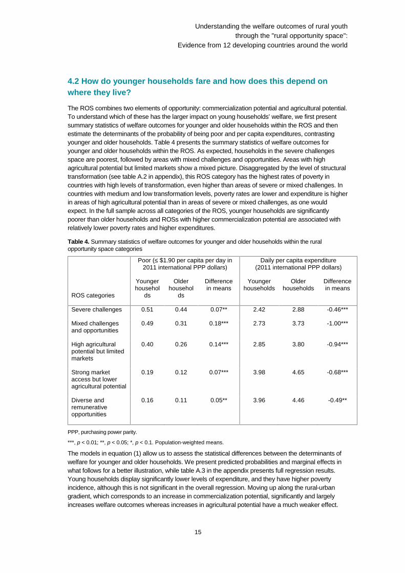
The ROS combines two elements of opportunity: commercialization potential and agricultural potential.To understand which of these has the larger impact on young households’ welfare, we first presentsummary statistics of welfare outcomes for younger and older households within the ROS and thenestimate the determinants of the probability of being poor and per capita expenditures, contrastingyounger and older households. Table 4 presents the summary statistics of welfare outcomes foryounger and older households within the ROS. As expected, households in the severe challengesspace are poorest, followed by areas with mixed challenges and opportunities. Areas with highagricultural potential but limited markets show a mixed picture. Disaggregated by the level of structuraltransformation (see table A.2 in appendix), this ROS category has the highest rates of poverty incountries with high levels of transformation, even higher than areas of severe or mixed challenges. Incountries with medium and low transformation levels, poverty rates are lower and expenditure is higherin areas of high agricultural potential than in areas of severe or mixed challenges, as one wouldexpect. In the full sample across all categories of the ROS, younger households are significantlypoorer than older households and ROSs with higher commercialization potential are associated withrelatively lower poverty rates and higher expenditures.

Table 4. Summary statistics of welfare outcomes for younger and older households within the ruralopportunity space categories

ROS categories

Poor (≤ $1.90 per capita per day in2011 international PPP dollars)

Daily per capita expenditure(2011 international PPP dollars)

Youngerhousehol

ds

Olderhousehol

ds

Differencein means

Youngerhouseholds

Olderhouseholds

Differencein means

Severe challenges 0.51 0.44 0.07** 2.42 2.88 -0.46***

Mixed challengesand opportunities

0.49 0.31 0.18*** 2.73 3.73 -1.00***

High agriculturalpotential but limitedmarkets

0.40 0.26 0.14*** 2.85 3.80 -0.94***

Strong marketaccess but loweragricultural potential

0.19 0.12 0.07*** 3.98 4.65 -0.68***

Diverse andremunerativeopportunities

0.16 0.11 0.05** 3.96 4.46 -0.49**

PPP, purchasing power parity.

***, p < 0.01; **, p < 0.05; *, p < 0.1. Population-weighted means.

The models in equation (1) allow us to assess the statistical differences between the determinants ofwelfare for younger and older households. We present predicted probabilities and marginal effects inwhat follows for a better illustration, while table A.3 in the appendix presents full regression results.Young households display significantly lower levels of expenditure, and they have higher povertyincidence, although this is not significant in the overall regression. Moving up along the rural-urbangradient, which corresponds to an increase in commercialization potential, significantly and largelyincreases welfare outcomes whereas increases in agricultural potential have a much weaker effect.


16

Young households face similar levels of poverty probabilities in areas with the lowest potential on bothdimensions of the ROS (figure 5). However, the decline is much larger as commercialization potential(figure 5a) increases compared with agricultural potential (figure 5b).

Figure 5. Predicted probabilities of being poor for younger and older households depending on their locationalong the axes of the rural opportunity space: (a) agricultural potential; (b) commercialization potential



17

Notes: Predicted probabilities with confidence intervals from probit regressions as specified in equation (1).Regression results are presented in table A.3. Controls are the agricultural potential, commercialization potential,proportion of secondary schooling among working-age household members, whether the household head is female,interaction of the young household dummy with these covariates and country dummies.

Regional differences not presented here show that, in African countries, the predicted probability ofbeing poor for young households is on average 42 per cent in rural hinterland areas, falling drasticallyto 9 per cent in urban areas, an almost fivefold decline. In Asia, the decline from rural to urban areas isaround eight times and in LAC three times, but in both regions at much lower levels of poverty than inAfrica. Although the interaction variables between the ROS and young household indicator bythemselves are not significant in the regression, the combined effect of being a mostly youngerhousehold and location is expected to be significant, as the confidence intervals in the figures 5 a) andb) above indicate. Thus, we take the total derivatives of being a young household in a specificcategory of the commercialization potential and we predict the marginal effects at the means for the fullsample as well as for each structural transformation group (table 5). We find that young households’welfare outcomes differ significantly across levels of structural transformation of the national economy.The overall disadvantage of being a mostly younger household compared with a mostly olderhousehold is largest in least transformed countries, with an expenditure gap of 46 per cent in ruralhinterland areas falling to 16 per cent in urban areas. In the most transformed countries of our sample,the young household penalty is insignificant in every category. In the middle ground, youngerhouseholds are significantly disadvantaged but the gap in rural and semirural areas is less than half ofthe gap in the least transformed countries, yet it is similar in the peri-urban and urban areas.


18

Table 5. Marginal effects of being a young household, by level of structural transformation (ST) and rural-urban gradient

Level ofstructuraltransformation

Rural andyoung

Semirural andyoung

Peri-urban andyoung

Urban andyoung

% decrease in income (expenditure per capita)

ST high 26 19 21 17

ST medium 14*** 18*** 27*** 15***

ST low 46*** 37*** 26*** 16***

Full sample 28*** 26*** 23*** 16***

Percentage point difference in probability of being poor

ST high 0 -1 0 -1

ST medium -14*** -12*** 3 -11***

ST low 30*** 35*** 35*** 38***

Full sample 15 18** 16* 15

Notes: ***, p < 0.01; **, p < 0.05; *, p < 0.1. Marginal effects are computed from separate regressions of youngerand older households. Changes are computed based on marginal effect at the mean of being a mostly youngerhousehold and living in a rural, semirural, peri-urban or urban area, holding all other variables constant. Othercontrols are the agricultural potential, commercialization potential, proportion of secondary schooling amongworking-age household members, whether the household head is female and country dummies.

These patterns are somewhat different with regard to the likelihood of being poor (lower panel oftable 5). It appears that younger households are overall significantly more likely to be poor than olderhouseholds, yet with little variation across rural-urban categories but a stark difference between levelsof transformation. Similarly to the case for expenditure, there is no significant young household penaltyin any category of the rural-urban gradient in the most transformed countries. The countries with amedium level of transformation include Nicaragua and Bangladesh, which have very differentpopulation densities and poverty levels, hence when combined in poverty analysis using theinternational poverty line they reveal a surprising penalty for older households even though youngerhouseholds were disadvantaged in terms of expenditure. The least transformed countries show largeand significant differences in poverty incidence between younger and older households, from 30percentage points in rural to 38 percentage points in urban areas. While commercialization potentialhelps to reduce the income gap between younger and older households, it does not seem to besufficient to lift younger households out of poverty in these countries. These results underline theimportance of the overall development of the broader economy as well as investments in connectivityto address the livelihood challenges rural youth face.

4.3 Exploring potential correlates of welfare outcomes

The finding that younger households tend to have lower expenditures per capita and to be more likelyto be poor than older households, especially in more remote areas, may be driven by a set of variablesthat capture the potentially differential access to productive assets and livelihood options. In thissubsection, we explore the roles of education, land ownership, credit access, income diversificationand commercialization in driving welfare outcomes (see summary statistics in table 3). One importantdriver of welfare outcomes is education, and especially secondary education is promising high returns



19

in developing countries (Shimeles, 2016). Having more economically active members with secondaryschooling is thus expected to improve household welfare. The average proportion of working-agehousehold members with secondary schooling in our sample is 0.29 for younger and 0.37 for olderhouseholds, indicating a disadvantage for younger households. To test the effect of increasingsecondary schooling, we run separate regressions for only younger or only older households andestimate the percentage point change in per capita expenditure and poverty incidence of adding onemore working-age member with secondary education (table 6). Overall, it seems that older householdsgain relatively more than younger households from secondary education in terms of per capitaexpenditure increase, with the exception of households in most transformed countries. This indicatesother constraints and challenges for younger households to realize their potential aside fromeducation. By level of transformation, the largest increases in per capita expenditure could be found inthe sample of countries with medium and low levels of transformation. Within countries, expendituregains from education are estimated to be largest in semirural and peri-urban areas; less so in veryremote areas, especially for younger households.

Table 6. Increasing the number of working-age household members with secondary schooling by oneperson: changes in expenditure and poverty

Fullsample

Rural-urban gradient By level of structuraltransformation

Rural Semirural Peri-urban

Urban High Medium Low

Percentagepointchange inexpenditure

Youngerhouseholds

23*** 16** 25*** 24*** 19*** 25** 36* 21**

Olderhouseholds

34*** 29*** 31*** 36*** 22*** 20** 46** 31***

Difference -10 -13 -6 -12 -4 5 -10 -10

Percentagepointchange inpovertyincidence

Youngerhouseholds

-7*** -9*** -10*** -5*** -2*** -4*** -6*** -9***

Olderhouseholds

-6*** -10*** -9*** -5*** -2*** -3*** -1*** -12***

Difference -1 1 -1 0 0 -1 -6 2

Notes: ***, p < 0.01; **, p < 0.05; *, p < 0.1. Changes are computed based on marginal effect of increasingproportion of working-age household members with schooling from the mean to the proportion that reflects onemore working-age person with secondary schooling in the household, holding all other variables constant.Regressions are run separately for younger and older households. Other controls are the agricultural potential,commercialization potential and whether the household head is female.

In contrast, the decline in poverty incidence due to more education appears to affect younger andolder households equally across the rural-urban gradient. The effect is largest in the least transformedcountries and in the most remote areas. Having one more working-age member with secondaryeducation would reduce the likelihood of being poor by 9 or 12 percentage points for younger or olderhouseholds respectively in the least transformed countries. In the most remote areas poverty isrelatively high (above 50 per cent for younger households) and having one more household memberwith secondary schooling is associated with a 9 percentage point decline in the likelihood of being apoor household. These results point to the potential returns to education in these areas, even thoughin the most remote areas opportunities to realize these returns might be sparse, which these results donot take into account.


20

Younger households may also face greater constraints on accessing land to farm, especially duringthe demographic transition phase, during which age of inheritance is delayed by low death rates butthe birth rates remain high (Stecklov and Menashe-Oren, 2019) and in places where land markets areconstrained with little rental activity (Kwame Yeboah et al., 2019). More remote areas present otherchallenges due to lack of connections to markets (e.g. for outputs or credit) and other livelihoodopportunities. Table 7 presents the prevalence of land ownership, credit access and income sharesfrom farming and farm sales by country group and household category, revealing interesting patterns.

Table 7. Land ownership, access to credit and income sources of younger and older households by level oftransformation

Household characteristics Youngerhouseholds

Olderhouseholds

Difference inmeans

High ST


Land per capita, in hectare (for thoseowning) 0.58 0.82 -0.24***

Household has received any credit,dummy 0.33 0.34 -0.01


Share of sales in own farm income 0.30 0.27 0.03***

Medium ST

Land ownership, dummy 0.39 0.45 -0.06***

Land per capita, in hectare (for thoseowning) 0.14 0.18 -0.04**

Household has received any credit,dummy 0.35 0.28 0.07***

Farming share of total income 0.23 0.25 -0.02**

Share of sales in own farm income 0.37 0.36 0.01

Low ST


Land per capita, in hectare (for thoseowning) 0.24 0.19 0.05***

Household has received any credit,dummy 0.20 0.19 0.01


Share of sales in own farm income 0.29 0.32 -0.02**

ST: structural transformation

Notes: Authors’ calculation based on household survey data from 12 countries. ***, p < 0.01; **, p < 0.05; *, p < 0.1.Population-weighted means. Information on land area is not available for Mexico. Information on credit availability is notavailable for Nicaragua and Peru.



21

Younger households are more likely to own land than older households in all country groups but themedium-level countries, where they are 6 percentage points less likely to own land. Overall, landownership is very low in the most transformed (Latin American) sample, as land consolidation andmovement out of agriculture are highly correlated with structural transformation. The gap betweenyounger and older households in terms of size of the land owned relative to household size, incontrast, is strikingly large in these transformed economies. While relatively more younger householdsown land, older households own on average 0.24 hectares more than younger households in percapita terms. Within the ROS presented in table A.4 in the appendix, this gap is primarily found inspaces with mixed challenges and opportunities, but also in those with high agricultural potential,putting younger households at a disadvantage in making the most of the most productive land in theseotherwise relatively rich economies. In the least transformed countries, younger households do notseem to face a disadvantage in accessing land independent of their position within the ROS(see appendix table A.4).

There is no indication of a disadvantage for younger households in accessing credit, but credit accessis very low (around 20 per cent) in the least transformed countries, whereas a third of households inthe other two regions have received credit. In terms of the importance of farming for incomegeneration, only a few households in the most transformed countries appear to depend on farming astheir primary income source, as one would expect in these economies. In mid-level transformedeconomies, farming comprises around a quarter of household income, for younger and for olderhouseholds. In the low-transformation countries, younger households’ income depends significantly onfarming, with 50 per cent of income compared with 30 per cent for older households, but bothhousehold types commercialize their products, with around 30 per cent of their farm income generatedthrough sales. In the high-transformation countries, households that have a farm sell similarproportions. In the medium-transformation countries, younger and older farming households alike gainalmost 40 per cent of their farm income from sales, pointing to a higher commercialization potentialincluding in areas with agricultural potential.

Along the rural-urban gradient, table 8 confirms expected patterns. Land ownership is most common inrural areas, more so among younger households, but they own smaller areas. Land size declines withpopulation density, while access to credit increases with it. Farming contributes most to incomes inrural areas, especially for younger households, but still comprises a quarter of household incomes inperi-urban areas. Interestingly, the proportion of farm income coming from sales is around a third inrural, semirural and peri-urban areas, with a small difference between younger and older households,although there is a slightly higher proportion of farm income from sales in peri-urban than rural areas.This finding, combined with the observation that the proportion of total income from farming is muchlower in these areas, suggests that improvements in connectivity over the ROS mostly explain incomediversification rather than farm commercialization.13 While farming appears to contribute an importantproportion of younger households’ income, they do not seem to be able to achieve high income from it,potentially because of the lack of connectivity.

_______________________________13 Note that table 8 does not differentiate between processed and non-processed farm sales, and that processing offarm produce is found to be higher in secondary cities and small towns than in remote areas (Reardon, 2015).


22

Table 8. Land ownership, access to credit and income sources of younger and older households by rural-urban gradient

Household characteristicsYounger

householdsOlder households Difference in

means

Rural hinterland


Land per capita, in hectare (for thoseowning)

0.40 0.53 -0.14***

Household has received any credit, dummy 0.19 0.17 0.01


Share of sales in own farm income 0.30 0.32 -0.02

Semirural



0.20 0.16 0.04***



Share of sales in own farm income 0.29 0.33 -0.04***

Peri-urban



0.14 0.15 -0.01


Farming share of total income 0.25 0.23 0.02*

Proportion of sales in own farm income 0.34 0.36 -0.02

Notes: Authors’ calculation based on household survey data from 12 countries. ***, p < 0.01; **, p < 0.05; *, p < 0.1.Population-weighted means. Information on land area is not available for Mexico. Information on credit availability is notavailable for Nicaragua and Peru.



23

5. Conclusion

Where do rural youth live, what challenges or opportunities do the areas where they live provide andhow are these associated with welfare outcomes? The current policy debate around the youthchallenge in developing countries lacks robust evidence addressing these questions. This study(resulting from extensive analytical work for the Rural Development Report 2019) offers such evidenceat the global and household levels by drawing on innovative use of geo-spatial data combined withnationally representative household data from 12 countries. Conceptualizing youth’s challenges andopportunities in the national, geographical and family contexts, we assess how these contexts shaperural (non-urban) youth’s welfare outcomes. The level of structural transformation of the nationaleconomy is expected to broaden or narrow the opportunities for rural youth in more or lesstransformed countries respectively, resulting in lower or higher youth penalties in welfare outcomes.The level of commercialization and agricultural potential of a location within a country forms the ROSof rural youth, while the demographic structure of a household is expected to ease or complicateyouth’s transition into adulthood in older or younger households respectively.

By combining the results of our descriptive and regression analyses we provide a rich account ofwhere rural youth live and how this shapes their welfare outcomes, highlighting the importance of aspatially disaggregated approach to policy prioritization to include them. The results indicate thatconnectivity (commercialization potential) and education play a significant role in poverty reduction foryoung households, which seem to fare worse overall than older households. The gaps betweenyounger and older households and between less and more educated young households are starkestin the least transformed countries, of which the majority are in sub-Saharan Africa.

These findings point to heterogeneity in investment priorities depending on the level of transformationof a country and the opportunity space rural youth live in within the country. As discussed extensivelyin the RDR 2019 (IFAD, 2019) and supported by the results of this paper, countries with low levels oftransformation should focus on improving fundamental capabilities in rural areas, among themespecially infrastructure and education to improve youth livelihoods and enable rural transformation.More transformed economies face the challenge of ensuring that the transformation of their rural areasdoes not lag behind and is inclusive of rural youth, avoiding pockets of poverty.

24

ReferencesAbay, K., W. Asnake, H. Ayalew, J. Chamberlin and J. Sumberg. 2019. Landscapes of opportunity?

How young people engage with the rural economy in sub-Saharan Africa. Background paper forthe Rural Development Report 2019. Rome: IFAD.

Alegana, V. A., P. M. Atkinson, C. Pezzulo, A. Sorichetta, D. Weiss, T. Bird, E. Erbach-Schoenbergand A. J. Tatem. 2015. Fine resolution mapping of population age-structures for health anddevelopment applications. Journal of the Royal Society Interface 12: 20150073.

Bilsborrow, R. E. 1987. Population pressures and agricultural development in developing countries: Aconceptual framework and recent evidence. World Development 15(2): 183-203.

Carletto, G., K. Covarrubias, B. Davis, M. Krausova and P. Winters. 2008. Rural Income GeneratingActivities study: Methodological note on the construction of income aggregates. Rome: FAO.

Chivasa, Walter, Onisimo Mutanga and Chandrashekhar Biradar. 2017. Application of remote sensingin estimating maize grain yield in heterogeneous African agricultural landscapes: A review.International Journal of Remote Sensing 38(23): 6816-6845. doi:10.1080/01431161.2017.1365390.

Christiaensen, L., J. De Weerdt and Y. Todo. 2013. Urbanization and poverty reduction: The role ofrural diversification and secondary towns. Agricultural Economics 44(4-5): 435-447.

Davis, B., S. Di Giuseppe and A. Zezza. 2017. Are African households (not) leaving agriculture?Patterns of households’ income sources in rural Sub-Saharan Africa. Food Policy 67: 153-174.

Dolislager, M., D. Tschirley, T. Reardon, A. Arslan, L. Fox, S. Liverpool-Tasie, B. Minten. 2019.Agrifood system employment in overall youth vs adult employment in Africa, Asia, and LatinAmerica: The view from LSMS survey data on individuals. Background paper for the RuralDevelopment Report 2019. Rome: IFAD.

Doss, C., J. Heckert, E. Myers, A. Pereira and A. Quisumbing. 2019. Gender, rural youth, andstructural transformation. Background paper for the Rural Development Report 2019. Rome:IFAD.

Gaughan, A.E., F.R. Stevens, C. Linard, P. Jia and A.J. Tatem. 2013. High-Resolution PopulationDistribution Maps for Southeast Asia in 2010 and 2015. PLoS One, 8.

Ghani, Ejaz, ed. 2010. The poor half billion in South Asia: What is holding back lagging regions? NewDelhi: Oxford University Press.

Gibson, J., G. Datt, R. Murgai and M. Ravallion. 2017. For India’s rural poor, growing towns mattermore than growing cities. World Development 98: 413-429.

IFAD. 2016. Rural development report 2016: Fostering inclusive rural transformation. Rome: IFAD.

IFAD. 2019. Rural development report 2019: Creating opportunities for rural youth. Rome: IFAD.

25

Jaafar, Hadi H. and Farah A. Ahmad. 2015. Crop yield prediction from remotely sensed vegetationindices and primary productivity in arid and semi-arid lands. International Journal of RemoteSensing 36(18): 4570-4589. doi: 10.1080/01431161.2015.1084434.

Jones, A., Y. Acharya and L. Galway. 2016. Urbanicity gradients are associated with the household-and individual-level double burden of malnutrition in sub-Saharan Africa. Journal of Nutrition146(6): 1257-1267.

Kwame Yeboah, F., T. S. Jayne, M. Muyanga and J. Chamberlin. 2019. The intersection of youthaccess to land, migration, and employment opportunities: Evidence from sub-Saharan Africa.Background paper for the Rural Development Report 2019. Rome: IFAD.

Lerner, A. M. and H. Eakin. 2010. An obsolete dichotomy? Rethinking the rural-urban interface interms of food security and production in the global south. Geographical Journal 177(4): 311-320.

Reardon, T. 2015. The hidden middle: The quiet revolution in the midstream of agrifood value chainsin developing countries. Oxford Review of Economic Policy 31(1): 45-63.

Ripoll, S., J. Andersson, L. Badstue, M. Büttner, J. Chamberlin, O. Erenstein and J. Sumberg. 2017.Rural transformation, cereals and youth in Africa: What role for international agriculturalresearch? Outlook on Agriculture 46(3): 168-177. doi: 10.1177/0030727017724669.

Roberts, B., and R. P. Hohmann. 2014. The systems of secondary cities: The neglected drivers ofurbanising economies. CIVIS Sharing Knowledge and Learning from Cities No 7. Washington,D.C.: World Bank.

Shimeles, A. 2016. Can higher education reduce inequality in developing countries? IZA World ofLabor 2016: 273. doi: 10.15185/izawol.273.

Simon, D. 2008. Urban environments: issues on the peri-urban fringe. Annual Review ofEnvironmental Resources 33: 167-185.

Simon, D., D. McGregor and D. Thompson. 2006. Contemporary perspectives on the peri-urbanzones of cities in developing countries. In The peri-urban interface: Approaches to sustainablenatural and human resource use, edited by D. McGregor, D. Simon and D. Thompson, 3-17.London: Earthscan.

Stecklov, G., and A. Menashe-Oren. 2019. The demography of rural youth in developing countries.Background paper for the Rural Development Report 2019. Rome: IFAD.

Stevens, F.R., A.E. Gaughan, C. Linard and A.J. Tatem. 2015. Disaggregating Census Data forPopulation Mapping Using Random Forests with Remotely-Sensed and Ancillary Data. PLoSOne, 10:e0107042.

Tatem, A.J., A.M. Noor, C. von Hagen, A. Di Grigorio and S.I. Hay. 2007. High-Resolution PopulationMaps for Low-Income Nations: Combining land cover and census in East Africa. PLoS One, 2:34-36.

UNDESA. 2017. Population prospects: The 2017 revision. New York: United Nations PopulationDivision.

26

Webster, D. 2002. On the edge: Shaping the future of peri-urban East Asia. Stanford, CA: StanfordUniversity.

Wiggins, S., and S. Proctor. 2001. How special are rural areas? The economic implications of locationfor rural development. Development Policy Review 19(4): 427-436.

Wood, L. J. 1974. Population density and rural market provision. Cahiers d’études Africaines 14(56):715-726.

World Bank. 2018a, World Bank Analytical Classifications: Historical classification by income,Washington, D.C.: World Bank.

World Bank. 2018b. World Development Report 2018: Learning to realize education’s promise.Washington, D.C.: World Bank.

27

Appendix A

Table A.1. Non-agricultural percentage of GDP in 12 study countries

Country Non-agricultural percentage ofGDP

Bangladesh 85

Cambodia 73

Ethiopia 63

Malawi 72

Mexico 96

Nepal 67

Nicaragua 83

Niger 59

Nigeria 79

Peru 92

Tanzania 68

Uganda 74

Note: The tercile thresholds are 78 per cent and 89 per cent.

Data source: World Development Indicators

28

Table A.2. Poverty incidence and expenditure of younger and older households within the ruralopportunity space, by level of structural transformation

Poor ($1.90 per capita per day in 2011international PPP dollars)

Daily per capita expenditure (2011international PPP dollars)

Rural opportunityspace

Youngerhouseholds

Olderhouseholds

Differencein means

Youngerhouseholds

Olderhouseholds

Differencein means

High STSevere challenges 0.11 0.13 -0.02 4.67 4.89 -0.22*Mixed challengesand opportunities

0.12 0.09 0.03*** 5.04 5.85 -0.81***


0.26 0.24 0.03* 3.87 4.06 -0.20*


0.08 0.07 0.02* 6.25 6.54 -0.30


0.17 0.13 0.04 4.50 4.75 -0.25

Medium STa

Severe challenges 0.00 0.03 -0.03 6.13 7.14 -1.02Mixed challengesand opportunities

0.10 0.11 -0.01 4.00 5.38 -1.37***


0.01 0.03 -0.02 4.24 6.06 -1.82***


0.14 0.09 0.04*** 3.48 4.23 -0.75***


0.09 0.08 0.01 3.44 4.34 -0.90***

Low STSevere challenges 0.58 0.53 0.05 2.02 2.21 -0.19

Mixed challengesand opportunities

0.54 0.37 0.17*** 2.41 3.14 -0.73***

High agricultural.potential but limitedmarkets

0.45 0.31 0.15*** 2.54 3.27 -0.73***


0.33 0.21 0.11*** 3.70 5.15 -1.44**


0.19 0.15 0.04 4.00 4.44 -0.44

PPP, purchasing power parity; ST, structural transformation.

***, p < 0.01; **, p < 0.05; *, p < 0.1. Point estimates are population means.

a, This group is formed of only two countries, of which one does not have any population categorized as living inareas with severe challenges (Bangladesh), so that the values presented for this category come from Nicaraguaonly.

29

Table A.3. Welfare regressions: expenditure and poverty regressed on the two variables of the ruralopportunity space and household characteristics

Per capita expenditure Poor (dummy)

Right-hand side variables Coef. S.E. Coef. S.E.

Young household (dummy) -0.059*** 0.016 0.036 0.025

Commercialization potential (Base =Urban)

Rural -0.507*** 0.046 0.231*** 0.034

Semirural -0.348*** 0.053 0.152*** 0.026

Peri-urban -0.193*** 0.047 0.081*** 0.021

Agricultural potential (3-year meanEVI) -0.034 0.234 -0.042 0.170

Share of adults with secondaryeducation 0.006*** 0.001 -0.003*** 0.000

Female household head 0.091*** 0.019 -0.052*** 0.014

Young household*Rural -0.006 0.049 -0.002 0.043

Young household*Semirural -0.062 0.034 0.031 0.025

Young household*Peri-urban -0.017 0.025 0.007 0.026

Young household*Ag. potential -0.016 0.144 -0.065 0.048

Young household*Secondaryeducation -0.001 0.001 0.001 0.000

Young household*Femalehousehold head -0.009 0.035 0.022*** 0.006

Constant 1.267*** 0.088

Country dummies Yes Yes

Number of observations 79 360 79 472

Adjusted R2 0.430

Notes: Per capita regression is ordinary least squares, poverty regression a probit estimation, and in both casesstandard errors were clustered at country level and population weights applied.

***, p < 0.01; **, p < 0.05; *, p < 0.1.

Coef., coefficient; S.E., standard error.

30

Table A.4. Land ownership of younger and older households within the rural opportunity space, by levelof transformation

Land ownership, dummy Land per capita, in hectare

Rural opportunity space Youngerhouseholds

Olderhouseholds

Differencein means

Youngerhouseholds

Olderhouseholds

Differencein means

High ST

Severe challenges 0.44 0.27 0.17*** 0.62 0.38 0.24***

Mixed challenges andopportunities

0.34 0.19 0.16*** 0.30 0.51 -0.20**

High agricultural potentialbut limited markets

0.57 0.39 0.18*** 0.95 1.46 -0.50***

Strong market access butlower agricultural potential

0.07 0.04 0.03*** 0.31 0.53 -0.23

Diverse and remunerativeopportunities

0.19 0.14 0.05* 0.21 0.00 0.21

Medium ST

Severe challenges 0.38 0.23 0.15 11.27 2.00 9.27


0.40 0.34 0.05 0.70 1.19 -0.50**


0.39 0.31 0.08 0.43 0.61 -0.19


0.44 0.52 -0.09*** 0.10 0.12 -0.02***


0.41 0.48 -0.07* 0.10 0.14 -0.04*

Low ST

Severe challenges 0.88 0.71 0.17*** 0.36 0.33 0.04


0.80 0.53 0.28*** 0.25 0.18 0.08***


0.86 0.66 0.20*** 0.22 0.18 0.04*


0.64 0.33 0.31*** 0.09 0.11 -0.02


0.74 0.46 0.28*** 0.13 0.13 0.00

***, p < 0.01; **, p < 0.05; *, p < 0.1. Point estimates are population means.

ST, structural transformation.

31

Table A.5. Population density thresholds and resulting average population density to define thecategories of the rural-urban gradient from global WorldPop data.

Pop. Density Threshold

(1,000 people per sqkm)

Average populationdensity

Rural <=0.16 0.05

Semi-rural >0.16 & <=0.58 0.32

Peri-Urban >0.58 & <=2.39 1.20

Urban >2.39 7.56

Table A.6. Distribution of youth: world quartiles compared to administrative rural definition by region.

Population density based rural-urban gradient

Administrative definition Rural Semi-Rural Peri-Urban Urban

LAC Urban 7.18 9.76 22.46 60.60

Rural 68.52 22.46 8.66 0.36

SSA Urban 6.90 36.25 26.83 30.03

Rural 45.95 35.36 15.40 3.28

APR Urban 0.15 4.05 45.22 50.58

Rural 7.61 16.46 70.53 5.40

32

Table A.7. Data sources for household level data.

Country Survey Name Source Year Geo-locationsSub-Saharan AfricaEthiopia Ethiopian Socioeconomic Survey Central Statistical Agency of Ethiopia - CSA 2015/2016 Enumeration

Areas (EA)geocoded

Malawi Fourth Integrated Household Survey National Statistical Office (NSO) - Ministry of Economic Planning andDevelopment (MoEPD)

2016/2017 EAs geocoded

Niger National Survey on Household LivingConditions on Agriculture - Panel

Survey and Census Division - National Institute of Statistics 2014 EAs geocoded

Nigeria General Household Survey- Panel National Bureau of Statistics (NBS) - Federal Government of Nigeria 2015/2016 EAs geocoded

Tanzania National Panel Survey National Bureau of Statistics - Ministry of Finance and Planning 2014/2015 EAs geocoded

Uganda The Uganda National Panel Survey Uganda Bureau of Statistics - Government of Uganda 2013/2014 EAs geocoded

Latin America

Mexico Encuesta nacional de ingresos y gastosde los hogares

Instituto Nacional de Estadística y Geografía, MEX-INEGI.40.202.03-ENIGH-2016-NS

2016 EAs geocoded

Nicaragua Encuesta nacional de hogares sobremedición de nivel de vida

Instituto Nacional de Información de Desarrollo 2014 Municipalitygeocodesidentified

Peru Encuesta nacional del hogares 2016(Anual) – Condiciones de vida y pobreza

Instituto Nacional de Estadística e Informática 2016 EAs geocoded

AsiaBangladesh Household Income and Expenditure

SurveyBangladesh Bureau of Statistics - Ministry of Planning 2010 Upazila geocodes

identifiedCambodia Cambodia Socio-Economic Survey National Institute of Statistics - Ministry of Planning 2014 Village geocodes

identifiedNepal Nepal Living Standards Survey Central Bureau of Statistics - National Planning Commission

Secretariat, Government of Nepal2010 Village geocodes

identified

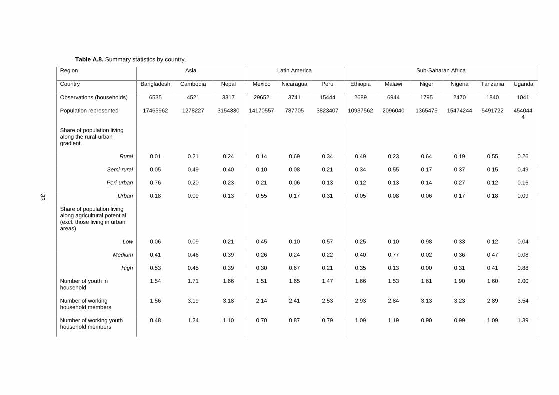
33

Table A.8. Summary statistics by country.

Region Asia Latin America Sub-Saharan Africa

Country Bangladesh Cambodia Nepal Mexico Nicaragua Peru Ethiopia Malawi Niger Nigeria Tanzania Uganda

Observations (households) 6535 4521 3317 29652 3741 15444 2689 6944 1795 2470 1840 1041

Population represented 17465962 1278227 3154330 14170557 787705 3823407 10937562 2096040 1365475 15474244 5491722 4540444

Share of population livingalong the rural-urbangradient

Rural 0.01 0.21 0.24 0.14 0.69 0.34 0.49 0.23 0.64 0.19 0.55 0.26

Semi-rural 0.05 0.49 0.40 0.10 0.08 0.21 0.34 0.55 0.17 0.37 0.15 0.49

Peri-urban 0.76 0.20 0.23 0.21 0.06 0.13 0.12 0.13 0.14 0.27 0.12 0.16

Urban 0.18 0.09 0.13 0.55 0.17 0.31 0.05 0.08 0.06 0.17 0.18 0.09

Share of population livingalong agricultural potential(excl. those living in urbanareas)

Low 0.06 0.09 0.21 0.45 0.10 0.57 0.25 0.10 0.98 0.33 0.12 0.04

Medium 0.41 0.46 0.39 0.26 0.24 0.22 0.40 0.77 0.02 0.36 0.47 0.08

High 0.53 0.45 0.39 0.30 0.67 0.21 0.35 0.13 0.00 0.31 0.41 0.88

Number of youth inhousehold

1.54 1.71 1.66 1.51 1.65 1.47 1.66 1.53 1.61 1.90 1.60 2.00

Number of workinghousehold members

1.56 3.19 3.18 2.14 2.41 2.53 2.93 2.84 3.13 3.23 2.89 3.54

Number of working youthhousehold members

0.48 1.24 1.10 0.70 0.87 0.79 1.09 1.19 0.90 0.99 1.09 1.39

34

Region Asia Latin America Sub-Saharan Africa

Country Bangladesh Cambodia Nepal Mexico Nicaragua Peru Ethiopia Malawi Niger Nigeria Tanzania Uganda

Youth household head 0.04 0.05 0.07 0.09 0.09 0.05 0.07 0.18 0.04 0.02 0.11 0.05

Age of household head 46.71 48.70 46.89 46.30 46.38 48.82 47.10 41.73 47.32 53.52 43.46 48.15

Female household head 0.13 0.21 0.24 0.27 0.37 0.26 0.26 0.28 0.14 0.18 0.29 0.33

Share of working agehousehold members withsecondary schooling

0.09 0.20 0.19 0.75 0.51 0.61 0.10 0.14 0.08 0.47 0.12 0.16

Poor ($1.90 per capita perday in 2011 PPP)

0.1 0.0 0.2 0.1 0.0 0.0 0.6 0.6 0.3 0.4 0.3 0.3

Daily per capita expenditure(in 2011 PPP)

4.11 7.31 3.06 5.51 7.93 8.38 1.81 2.13 3.19 3.28 3.79 3.20

Owns land 0.44 0.69 0.78 0.12 0.19 0.20 0.72 0.71 0.70 0.54 0.62 0.72

Land owned in hectare 0.23 1.02 0.48 0.00 2.92 0.56 0.95 0.43 3.84 0.48 1.49 0.88

Land owned per householdmember in hectare

0.11 0.31 0.12 3.15 0.63 0.24 0.14 0.79 0.13 0.40 0.19

Received credit 0.31 0.30 0.39 0.33 0.25 0.25 0.05 0.18 0.16 0.09

Share of income fromfarming

0.24 0.35 0.50 0.06 0.20 0.07 0.57 0.53 0.36 0.34 0.39 0.43

Share of farm income sold 0.37 0.38 0.36 0.24 0.23 0.41 0.27 0.19 0.19 0.29 0.35 0.35

35

Table A.9. Share of all youth within the Rural Opportunity Space, as represented by the 12 householdsurveys and by the global data set of 85 low and middle income countries.

12 surveys Global

Severe challenges 10% 4%

Mixed challenges and opp. 36% 20%

High ag. potential but limited markets 17% 43%

Strong market access but lower ag. potential 29% 9%

Diverse and remunerative opp. 7% 24%

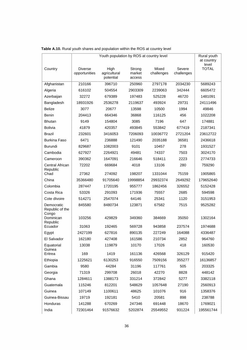
36

Table A.10. Rural youth shares and population within the ROS at country level

Youth population by ROS at country level Rural youthat country

levelCountry Diverse

opportunitiesHigh

agriculturalpotential

Strongmarketaccess

Mixedchallenges

Severechallenges

TOTAL

Afghanistan 210166 396710 250960 2797178 2034230 5689243

Algeria 616102 504554 2903309 2239063 342444 6605472

Azerbaijan 32272 679389 197483 525228 46720 1481091

Bangladesh 18931926 2536278 2119637 493924 29731 24111496

Belize 3077 20677 13598 10500 1994 49846

Benin 204413 664346 36868 116125 456 1022208

Bhutan 9149 154804 3085 7196 647 174881

Bolivia 41879 420357 493845 553842 677419 2187341

Brazil 232601 3416053 7206093 10036772 2721204 23612722

Burkina Faso 6471 236888 121490 2035188 36581 2436618

Burundi 829687 1082003 9101 10457 278 1931527

Cambodia 627927 2264921 49481 74337 7503 3024170

Cameroon 390362 1647091 216646 518411 2223 2774733

Central AfricanRepublic

72202 669684 4018 13106 280 759290

Chad 27362 274092 198207 1331044 75159 1905865

China 35366480 91705640 19998854 29932374 2649292 179652640

Colombia 287447 1720195 955777 1862456 326552 5152428

Costa Rica 53326 291093 171936 75557 2685 594598

Cote dIvoire 514271 2547074 64146 25341 1120 3151953

DemocraticRepublic of theCongo

845580 8480734 123871 67582 7515 9525282

DominicanRepublic

103256 429829 349360 384669 35050 1302164

Ecuador 31063 192465 569728 943858 237574 1974688

Egypt 2427199 627816 890135 227249 164088 4336487

El Salvador 162180 427408 161586 210734 2852 964760

EquatorialGuinea

13038 119879 10170 17026 418 160530

Eritrea 169 1419 161136 426568 326129 915420

Ethiopia 1225621 6130253 916550 7509156 355277 16136857

Gambia 9580 44284 31196 117761 505 203325

Georgia 71319 299708 26018 42270 8828 448142

Ghana 1284611 1388173 331214 372842 5277 3382118

Guatemala 115246 812201 548629 1057648 27190 2560913

Guinea 107149 1100611 48625 101076 916 1358376

Guinea-Bissau 19719 192181 5410 20581 898 238788

Honduras 141288 670269 247346 691448 18670 1769021

India 72301464 91576632 5202874 25549552 931224 195561744

37



opportunitiesHigh


Strongmarketaccess

Mixedchallenges

Severechallenges

TOTAL

Indonesia 15087535 16695277 408481 236514 29063 32456868

Iran 321974 1523821 1256647 7879547 6023107 17005096

Iraq 242699 435696 1524725 2799485 671984 5674590

Jordan 10943 50135 516490 367667 129165 1074400

Kazakhstan 39881 193786 376268 1810064 203445 2623444

Kenya 2633169 3477060 186470 1098911 79984 7475594

Kyrgyzstan 215263 178521 199074 344455 113871 1051184

Laos 70303 1043621 10229 14940 5418 1144511

Lesotho 0 1997 81344 411512 366 495219

Liberia 63649 553069 7440 3132 53 627343

Madagascar 30658 1791277 131117 1279254 4149 3236455

Malawi 204830 734185 383459 1871868 5966 3200308

Malaysia 443783 2099279 30605 18983 2680 2595331

Mali 3890 200821 143725 1389234 89735 1827405

Mauritania 0 249 54542 394454 100436 549681

Mexico 262336 2169381 5282843 4125938 2314798 14155296

Morocco 94974 373747 754300 2519310 396771 4139103

Mozambique 276563 3376338 171664 537826 5052 4367443

Myanmar 1629091 6146821 124893 599683 64825 8565313

Namibia 973 19490 97971 355075 20100 493609

Nepal 1477742 3196199 5918 51412 8910 4740182

Nicaragua 77400 413637 291088 493995 41720 1317840

Niger 0 1291 273460 1145962 203059 1623772

Nigeria 4038864 7561403 3405799 6746900 23214 21776180

Pakistan 5504903 12297474 947500 5694965 1744038 26188878

Paraguay 18546 240256 252435 481781 15300 1008318

Peru 2656 553915 702846 1137120 2159540 4556078

Philippines 4575359 7967001 154167 107556 9187 12813270

Republic ofCongo

38616 365742 15154 19175 301 438988

Rwanda 860275 1098370 21919 21973 1375 2003912

Senegal 11513 231113 293255 1529147 13642 2078671

Sierra Leone 56897 744813 11009 15040 737 828496

Somalia 47992 60556 399043 526301 34960 1068852

South Africa 1198463 2167132 2885224 3529253 36051 9816123

Sri Lanka 873267 1569083 11249 16517 2054 2472170

Suriname 3069 27779 20159 18418 2905 72330

Swaziland 28347 148127 3688 57299 169 237629

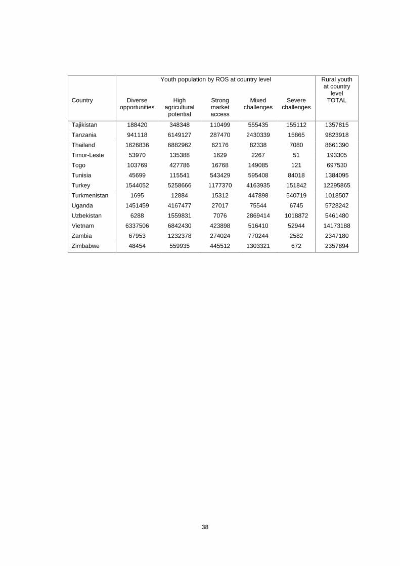
38



opportunitiesHigh


Strongmarketaccess

Mixedchallenges

Severechallenges

TOTAL

Tajikistan 188420 348348 110499 555435 155112 1357815

Tanzania 941118 6149127 287470 2430339 15865 9823918

Thailand 1626836 6882962 62176 82338 7080 8661390

Timor-Leste 53970 135388 1629 2267 51 193305

Togo 103769 427786 16768 149085 121 697530

Tunisia 45699 115541 543429 595408 84018 1384095

Turkey 1544052 5258666 1177370 4163935 151842 12295865

Turkmenistan 1695 12884 15312 447898 540719 1018507

Uganda 1451459 4167477 27017 75544 6745 5728242

Uzbekistan 6288 1559831 7076 2869414 1018872 5461480

Vietnam 6337506 6842430 423898 516410 52944 14173188

Zambia 67953 1232378 274024 770244 2582 2347180

Zimbabwe 48454 559935 445512 1303321 672 2357894

39

Appendix B

Methodological details for merging of global and household level data

1. Merging EVI and WorldPop data

For the agricultural potential axis of the ROS, Moderate Resolution Imaging SpectroradiometerEnhanced Vegetation Index (MODIS EVI) grids were resampled from 250m resolution to 1km using anearest neighbour algorithm to match the resolution of age-gender disaggregated WorldPop grids. EVIvalues were used only for land classified as cropland or pasture land. To do so, a new global map ofcropland / pasture was created by fusing two existing maps (Waldner et al. 2016; GFSAD 2010). Indoing so, the analysis was spatially targeted to agricultural land and production potential could beproxied for agricultural land. Finally, average EVI values for the 3-year period between 2013 and 2015were calculated to avoid seasonality and agro-climatic variation. EVI grids (same as WorldPop grids)were ordered from lowest to highest, and each of the three groups (terciles) hold one-third of all non-urban space and represent the low, medium, and high agricultural potential categories on thehorizontal axis.

2. Merging global EVI and WorldPop data with household survey data

Household data for Sub-Saharan Africa (SSA) come from the Living Standards Measurement Surveys- Integrated Surveys on Agriculture (LSMS-ISA) data, all of which provide geo-referenced information(i.e. the centroids) for each Enumeration Area (EA) in the sample. Using the number of dwellings andthe average household size in each EA, the total population of the average EA in each country wascalculated. Using the known population distribution from the WorldPop data, a boundary was thendrawn around the EA centroid to capture a population of this size, which created "artificial EAboundaries." The population density of each EA was calculated and then classified along thecategories of population density quartiles along the rural-urban gradient using the global threshold:Rural, Semi-Rural, Peri-Urban and Urban. The artificial boundaries created for each EA were alsoused to calculate the average value of the EVI for the 2013-2015 period (because most LSMS-ISAdata were collected in 2014 or 2015) as described above. An example map of Tanzania of theresulting overlay of population density categories and artificial boundaries of enumeration areas ispresented in below (Figure B.1).

For APR and LAC not all household data sources included geo-referenced information, thereforecentroids of municipalities or other small administrative units were used and in some cases boundaries(polygons) for relatively small administrative areas from DIVA were used to repeat the process aboveto create the ROS variables for each household. For our purposes, we have included any data set withboundary data for an administrative unit whose average size is 1,000 square km or less. This was thecase for Bangladesh (318 km2), Nepal (37 km2), Cambodia (115 km2) and Nicaragua (938km2).

40

Figure B.1. Map of Tanzania with enumeration areas and rural-urban gradient categorization of grids

List of RDR 2019 Background Papers published in IFAD Research Series

The demography of rural youth in developing countries By Guy Stecklov, Ashira Menashe-Oren

What drives rural youth welfare? The role of spatial, economic, and household factors By Aslihan Arslan, David Tschirley, Eva-Maria Egger

Youth agrifood system employment in developing countries: a gender-differentiated spatial approach

By Michael Dolislager, Thomas Reardon, Aslihan Arslan, Louise Fox, Saweda Liverpool-Tasie, Christine Sauer, David Tschirley

Gender, rural youth and structural transformation: Evidence to inform innovative youth programming

By Cheryl Doss, Jessica Heckert, Emily Myers, Audrey Pereira, Agnes Quisumbing

Rural outh inclusion, empowerment and participation By Carolina Trivelli, Jorge Morel

Economic participation of rural youth: what matters? By Louise Fox

Landscapes of rural youth opportunity By James Sumberg, Jordan Chamberlin, Justin Flynn, Dominic Glover and Vicky Johnson

Rural youth, today and tomorrow By Ben White

Climate and jobs for rural young people By Karen Brooks, Shahnila Dunston, Keith Wiebe, Channing Arndt, Faaiqa Hartley and Richard

Robertson

Rural transformation and the double burden of malnutrition among rural youth in developing countries

By Suneetha Kadiyala, Elisabetta Aurino, Cristina Cirillo, Chittur S. Srinivasan and Giacomo Zanello

Inclusive finance and rural youth By Arianna Gasparri, Laura Munoz

Information and communication technologies and rural youth By Jenny Aker

Youth access to land, migration and employment opportunities: evidence from sub-Saharan Africa

By Felix Kwame Yeboah, Thomas S. Jayne, Milu Muyanga and Jordan Chamberlin

Rural youth in the context of fragility and conflict By Ghassan Baliki, Tilman Brück (Team Leader), Neil T. N. Ferguson and Wolfgang Stojetz

Rural youth: determinants of migration throughout the world By Alan de Brauw

The Impact of Migrants’ Remittances and Investment on Rural Youth By Manuel Orozco, Mariellen Jewers

Unlocking the potential of rural youth: the role of policies and institutions By Lauren Phillips, Paola Pereznieto

Investing in rural youth in the Asia and the Pacific region By Roehlano Briones

https://www.ifad.org/ruraldevelopmentreport/download/

The rural youth situation in Latin America and the Caribbean By Maia Guiskin, Pablo Yanes, Miguel del Castillo Negrete

Investing in rural youth in the Near East, North Africa, Europe and Central Asia By Nader Kabbani

The narrative on rural youth and economic opportunities in Africa: Facts, myths and gaps By Athur Mabiso, Rui Benfica

All publications in the IFAD Research Series can be found at:

https://www.ifad.org/en/web/knowledge/series?mode=search&catSeries=39130673

https://www.ifad.org/en/web/knowledge/series?mode=search&catSeries=39130673

International Fund for Agricultural Development

Via Paolo di Dono, 44 - 00142 Rome, Italy

Tel: +39 06 54591 - Fax: +39 06 5043463

Email: [email protected]

www.ifad.org

facebook.com/ifad

instagram.com/ifadnews

linkedin.com/company/ifad

twitter.com/ifad

youtube.com/user/ifadTV

what drives rural youth welfare? the role of spatial

Documents