What is What is Business Business

Statistics?Statistics?

What Is Statistics?What Is Statistics?• Collection of DataCollection of Data

– Survey

– Interviews

• Summarization and Presentation of DataSummarization and Presentation of Data– Frequency Distribution

– Measures of Central Tendency and Dispersion

– Charts, Tables,Graphs

• Analysis of DataAnalysis of Data– Estimation

– Hypothesis Testing

• Interpretation of Data for use in Interpretation of Data for use in more Effective Decision-Makingmore Effective Decision-Making

Decision-Making

Descriptive StatisticsDescriptive Statistics• Involves

– Collecting Data

– Summarizing Data

– Presenting Data

• Purpose: Describe Data

InferentialInferential StatisticsStatistics• Involves Samples

– Estimation– Hypothesis Testing

• Purpose– Make Decisions About Population

Characteristics Based on a Sample

Key TermsKey Terms• Population (Universe)

– All Items of Interest

• Sample– Portion of Population

• Parameter– Summary Measure about Population

• Statistic– Summary Measure about Sample

• P in Population

& Parameter

• S in Sample & Statistic

CollectionCollection

of of

DataData

Data Types• Quantitative (categorical)

• Qualitative (numerical)– Discrete

– Continuous

1. Nominal Scale– Categories/Labels

• e.g., Male-Female– Data is nonnumeric or

numeric– No Arithmetic Operations– Count

2. Ordinal Scale– All of the above, plus– Ordering Implied

e.g., High-Low

Qualita

tive

3. Interval Scale– Equal Intervals– No True 0– Data is always numeric– e.g., Degrees Celsius– Arithmetic Operations– Multiples not meaningful

4. Ratio Scale– Properties of Interval Scale– True 0– Meaningful Ratios– e.g., Height in Inches

How AHow Arere Data Measured? Data Measured?

Quantit

ativ

e

Summarization Summarization andand

PresentationPresentation

ofof

Data Data

Data Presentation

• Ordered Array

• Stem and Leaf Display

• Frequency Distribution– Histogram

– Polygon

– Ogive

Stem-and-Leaf DisplayStem-and-Leaf Display

• Divide Each Observation into Stem Value and Leaf Value– Stem Value Defines

Class

– Leaf Value Defines Frequency (Count)

2 144677

3 028

4 1

Data: 21, 24, 24, 26, 27, 27, 30, 32, 38, 41

26

Time (in seconds) that 30 Randomly Selected CustomersSpent in Line of Bank Before Being Served

183 121 140 198 19990 62 135 60 175320 110 185 85 172235 250 242 193 75263 295 146 160 210165 179 359 220 170

183 121 140 198 19990 62 135 60 175320 110 185 85 172235 250 242 193 75263 295 146 160 210165 179 359 220 170

SECONDS Stem-and-Leaf Plot

Frequency Stem & Leaf

5.00 0 . 66789 5.00 1 . 12344 11.00 1 . 66777788999 4.00 2 . 1234 3.00 2 . 569 1.00 3 . 2 1.00 Extremes (>=359)

Stem width: 100 Each leaf: 1 case(s)

Frequency Distribution Table Frequency Distribution Table ExampleExample

Raw Data: 24, 26, 24, 21, 27, 27, 30, 41, 32, 38

Boundaries (Upper + Lower Boundaries) / 2

Width

Class Midpoint Frequency

15 but < 25 20 3

25 but < 35 30 5

35 but < 45 40 2

Rules for Constructing Rules for Constructing Frequency DistributionsFrequency Distributions

• Every score must fit into exactly one class (mutually exclusive)

• Use 5 to 20 classes

• Classes should be of the same width

• Consider customary preferences in numbers

• The set of classes is exhaustive

Frequency Distribution Table Frequency Distribution Table StepsSteps

1. Determine Range Highest Data Point - Lowest Data Point

2. Decide the Width (Number) of Each Class

3. Compute the Number (width) of Classes

Number of classes = Range / (Width of Class)

Width of classes = Range/(Number of classes)

3. Determine the lower boundary (limit) of the first class

4. Determine Class Boundaries (Limits)

5. Tally Observations & Assign to Classes

Time (in seconds) that 30 Randomly Selected CustomersSpent in Line of Bank Before Being Served

183 121 140 198 19990 62 135 60 175320 110 185 85 172235 250 242 193 75263 295 146 160 210165 179 359 220 170

Mean for Grouped DataNumber of

Customers

Time (in seconds) f

60 and under 120 6120 and under 180 10180 and under 240 8240 and under 300 4300 and under 360 2

30

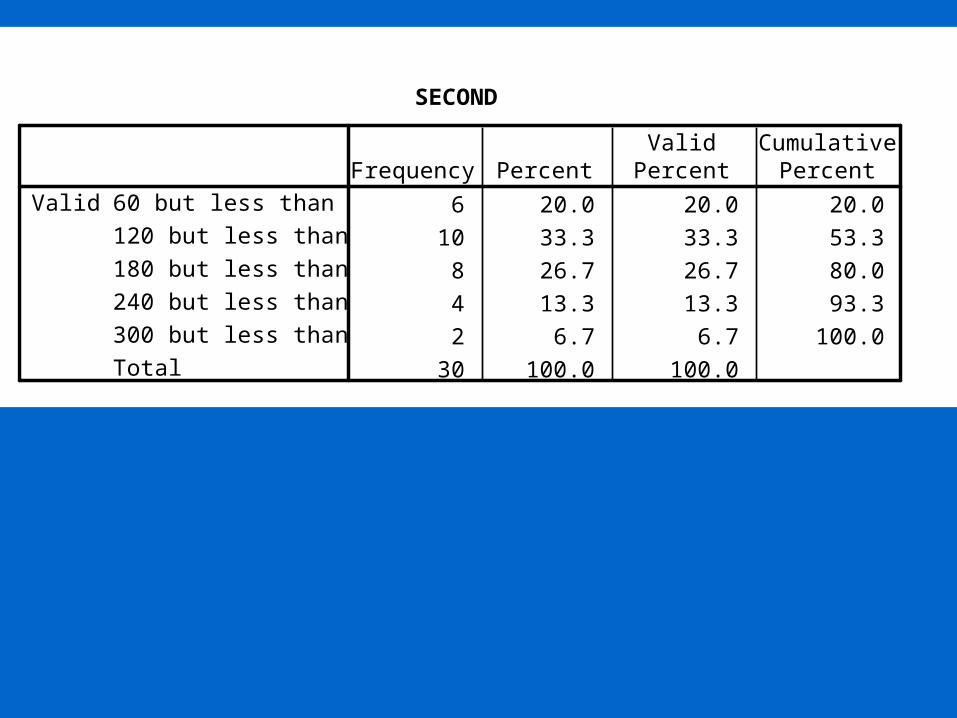
SECOND

6 20.0 20.0 20.0

10 33.3 33.3 53.3

8 26.7 26.7 80.0

4 13.3 13.3 93.3

2 6.7 6.7 100.0

30 100.0 100.0

60 but less than 120

120 but less than 180

180 but less than 240

240 but less than 300

300 but less than 360

Total

ValidFrequency Percent

ValidPercent

CumulativePercent

SECOND

54321

12

10

8

6

4

2

0

Std. Dev = 1.17

Mean = 3

N = 30.00

90 150 210 270 330

Fre

quen

cy

‘‘Chart Junk’Chart Junk’Good PresentationBad Presentation

Minimum Wage

0

2

4

1960 1970 1980 1990

$1960: $1.00

1970: $1.60

1980: $3.10

1990: $3.80

Minimum Wage

No Relative BasisNo Relative Basis

A’s by Class

0

100

200

300

FR SO JR SR

Freq.A’s by Class

0%

10%

20%

30%

FR SO JR SR

%

Bad Presentation Good Presentation

Compressing Compressing VerticalVertical AxisAxis

Quarterly Sales

0

100

200

Q1 Q2 Q3 Q4

$Quarterly Sales

0

25

50

Q1 Q2 Q3 Q4

$

Bad Presentation Good Presentation

No Zero Point No Zero Point on Vertical Axison Vertical Axis

Monthly Sales

0

20

40

60

J M M J S N

$Monthly Sales

36

39

42

45

J M M J S N

$

Bad PresentationGood Presentation

Standard NotationStandard Notation

Measure Sample Population

Mean X

Stand. Dev. S

Variance S2 2

Size n N

Numerical Data PropertiesNumerical Data Properties

Central Tendency (Location)

Variation (Dispersion)

Shape

Measures of Central Tendency Measures of Central Tendency forfor

Ungrouped DataUngrouped Data

Raw Data

MeanMean• Measure of Central Tendency

• Most Common Measure

• Acts as ‘Balance Point’

• Affected by Extreme Values (‘Outliers’)

• Formula (Sample Mean)

X

X

n

X X X

n

ii

n

n

1 1 2

Mean ExampleMean Example

• Raw Data: 10.3 4.9 8.9 11.7 6.37.7

XX X X X X X

n

X

n

ii

1 1 2 3 4 5 6

6

10 3 4 9 8 9 117 6 3 7 7

6

8 30

. . . . . .

.

Advantages of the MeanAdvantages of the Mean• Most widely used

• Every item taken into account

• Determined algebraically and amenable to algebraic operations

• Can be calculated on any set of numerical data (interval and ratio scale) -Always exists

• Unique

• Relatively reliable

Disadvantages of the Disadvantages of the MeanMean

• Affected by outliers

• Cannot use in open-ended classes of a frequency distribution

• Measure of Central Tendency

• Middle Value In Ordered Sequence– If Odd n, Middle Value of Sequence– If Even n, Average of 2 Middle Values

• Not Affected by Extreme Values

• Position of Median in Sequence

MedianMedian

Positioning Pointn 1

2

Median ExampleMedian Example Odd-Sized SampleOdd-Sized Sample

• Raw Data: 24.1, 22.6, 21.5, 23.7, 22.6

• Ordered: 21.5 22.6 22.6 23.7 24.1

• Position: 1 2 3 4 5

Positioning Point

Median

n 12

5 12

3 0

22.6

.

Median ExampleMedian Example Even-Sized SampleEven-Sized Sample

• Raw Data: 10.3 4.98.9 11.7 6.3 7.7

• Ordered: 4.9 6.3 7.7 8.9 10.311.7

• Position: 1 2 3 4 56Positioning Point

Median

n 12

6 12

3 5

7 7 8 92

8.3

.

. .

Advantages of the MedianAdvantages of the Median• Unique

• Unaffected by outliers and skewness

• Easily understood

• Can be computed for open-ended classes of a frequency distribution

• Always exists on ungrouped data

• Can be computed on ratio, interval and ordinal scales

Disadvantages of MedianDisadvantages of Median

• Requires an ordered array

• No arithmetic properties

ModeMode

• Measure of Central Tendency

• Value That Occurs Most Often

• Not Affected by Extreme Values

• May Be No Mode or Several Modes

• May Be Used for Numerical & Categorical Data

Advantages of ModeAdvantages of Mode• Easily understood

• Not affected by outliers

• Useful with qualitative problems

• May indicate a bimodal distribution

Disadvantages of ModeDisadvantages of Mode

• May not exist

• Not unique

• No arithmetic properties

• Least accurate

ShapeShape

• Describes How Data Are Distributed

• Measures of Shape– Skew = Symmetry

Symmetric

Mean = Median = Mode

Right-Skewed

Mode Median Mean

Left-SkewedMean Median Mode

Return on StockReturn on Stock

1998

1997

1996

1995

1994

10%

8

12

2

8

17%

-2

16

1

8

Stock X Stock Y

40% 40%

Average Return

on Stock= 40 / 5 = 8%

Measures of Dispersion Measures of Dispersion forfor

Ungrouped DataUngrouped Data

Raw Data

RangeRange• Measure of Dispersion

• Difference Between Largest & Smallest Observations

• Ignores How Data Are Distributed

Range X Xl est smallestarg

7 8 9 10 7 8 9 10

Return on Stock

1998

1997

1996

1995

1994

10%

8

12

2

8

17%

-2

16

1

8

Stock X Stock Y

Range on Stock X = 12 - 2 = 10%

Range on Stock Y = 17 - (-2) = 19%

Variance & Variance & Standard DeviationStandard Deviation

• Measures of Dispersion

• Most Common Measures

• Consider How Data Are Distributed

• Show Variation About Mean (X or )

Sample Sample Standard Deviation Standard Deviation FormulaFormula

S S2

( X X )

n

i

i

n

2

1

1

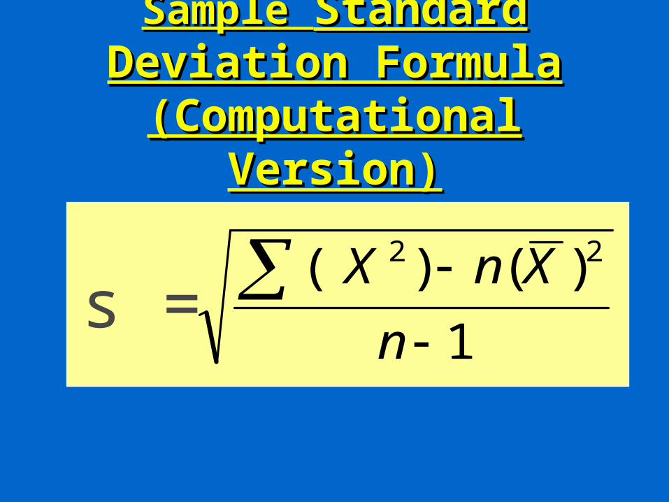
Sample Sample Standard Deviation Standard Deviation FormulaFormula

(Computational Version)(Computational Version)

1

)()( 22

n

XnXs =

Return on Stock

1998

1997

1996

1995

1994

10%

8

12

2

8

17%

-2

16

1

8

Stock X Stock Y

Range on Stock X = 12 - 2 = 10%

Range on Stock Y = 17 - (-2) = 19%

Standard Deviation of Stock X

X X ( X - X ) ( X - X )1998 10 8 2 41997 8 8 0 01996 12 8 4 161995 2 8 -6 361994 8 8 0 0

56

2

1

)( 2

n

XXs = = = = 3.74%

414

56

Return on Stock

1998

1997

1996

1995

1994

10%

8

12

2

8

17%

-2

16

1

8

Stock X Stock Y

40% 40%

Standard Deviation on Stock X = 3.74%

Standard Deviation on Stock Y = 8.57%

Population Mean

N

x

PopulationStandard Deviation

N

x

2)(

Coefficient of VariationCoefficient of Variation

• 1. Measure of Relative Dispersion

• 2. Always a %

• 3. Shows Variation Relative to Mean

• 4. Used to Compare 2 or More Groups

• 5. Formula (Sample)CV

S

X 100%

PopulationCoefficient of Variation

%100

popCV

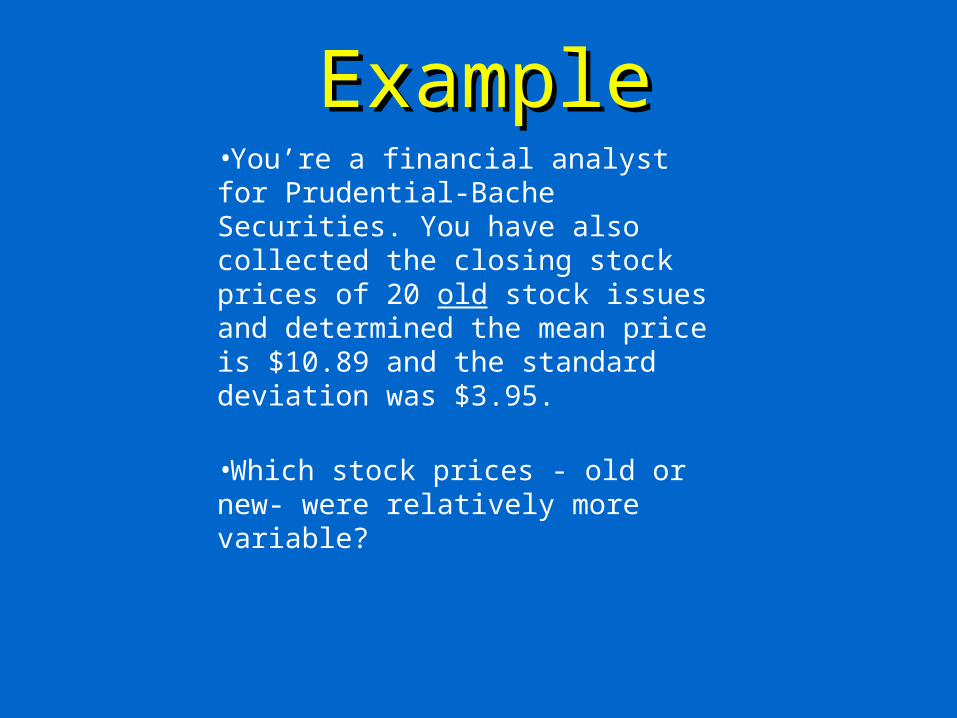
ExampleExample•You’re a financial analyst for Prudential-Bache Securities. You have also collected the closing stock prices of 20 old stock issues and determined the mean price is $10.89 and the standard deviation was $3.95.

•Which stock prices - old or new- were relatively more variable?

Comparison of CV’sComparison of CV’s

• Coefficient of Variation of new stocks

Coefficient of Variation of old stocks

CVS

X 100%

34

15 5100% 215%

3.34

..

CVS

X 100%

10.89100% 36.3%

3.95