what is value-at-risk, and is it appropriate for property/liability insurers? neil d. pearson...
TRANSCRIPT

What is Value-at-Risk, and Is It Appropriate for Property/Liability
Insurers?Neil D. Pearson
Associate Professor of Finance
University of Illinois at Urbana-Champaign
12-13 April 1999

What is Value-at-Risk?
0
5
10
15
20
25
P/L
< -
130
-11
0 <
P/L
<-9
0
-70
< P
/L <
-50
-30
< P
/L <
-10
10
< P
/L <
30
50
< P
/L <
70
90
< P
/L <
110
P/L
> 1
30
Hypothetical Daily Mark-to-Market Profit/Loss on Forward Contract (in $thousands)
Fre
quen
cy
value at risk(using x=5%)

If You Like the Normal Distribution
0.0
-150,000 -75,000 0 75,000 150,000
Mark-to-Market Portfolio Profit/Loss
Freq
uenc
y
5% 1.65 std. dev.
Value at risk: $86,625

What is Value-at-Risk?• Notation:
V change in portfolio value
f(V) density of V
x specified probability, e.g. 0.05
• Value-at-risk (VaR) satisfies
orx f V d V
( )
VaR
VaR
1
x f V d V( )

What is Value-at-Risk?
• Value-at-risk (for a probability of x percent) is the x percent critical value
• If you like the normal distribution, it is proportional to the portfolio standard deviation

What is Value-at-Risk?
• Value-at-risk is something you already understand• Value-at-risk is a particular way of summarizing
the probability distribution of changes in portfolio value
• The language of Value-at-Risk eases communication

If Value-at-Risk Isn’t New, Why Is It So Fashionable?
• It provides some information about a firm’s risks• It is a simple, aggregate measure of risk• It is easy to understand• “Value” and “risk” are business words

Basic Value-at-Risk Methodologies
• 3 methodologies:– Historical simulation
– Variance-covariance/Delta-Normal/Analytic
– Monte Carlo simulation
• Illustrate these using a forward contract– current date is 20 May 1996
– in 91 days (19 August)• receive 10 million
• pay $15 million

First step: Identify market factors
USD mark - to - market value =GBP million
1 +
USD million
1 +GBP USD
Sr r
10
91 360
15
91 360( / ) ( / )
Market factors: S, rGBP, and rUSD
PositionCurrent $ Value ofPosition
Cash Flow onDelivery Date
Long position in 91 day denominatedzero coupon bond with face value of 10million
S+r ( / )
GBP million
GBP
10
1 91360
Receive 10million
Short position in 91 day $ denominatedzero coupon bond with face value of $15million
USD 15 million
USD1 91360+r ( / )
Pay $15 million
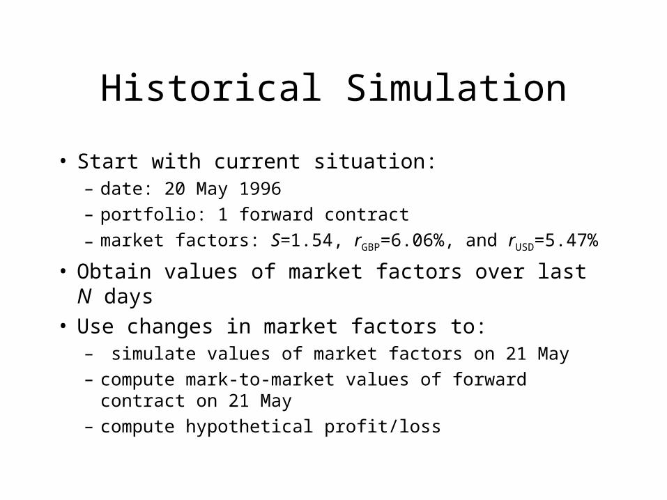
Historical Simulation
• Start with current situation:– date: 20 May 1996– portfolio: 1 forward contract
– market factors: S=1.54, rGBP=6.06%, and rUSD=5.47%
• Obtain values of market factors over last N days• Use changes in market factors to:
– simulate values of market factors on 21 May– compute mark-to-market values of forward contract on 21
May– compute hypothetical profit/loss

Historical simulation: P/LTable 1: Calculation of Hypothetical 5/21/96 Mark-to-Market Profit/Loss on aForward Contract Using Market Factors from 5/20/96 and Changes in Market Factorsfrom the First Business Day of 1996
Market FactorsMark-to-Market Value
$ Interest Rate(% per year)
Interest Rate(% per year)
ExchangeRate($/ )
of ForwardContract($)
Start with actual values ofmarket factors and forwardcontract as of close of businesson 5/20/96:
(1) Actual values on 5/20/96 5.469 6.063 1.536 327,771
Compute actual past changesin market factors:
(2) Actual values on 12/29/95 5.688 6.500 1.553
(3) Actual values on 1/2/96 5.688 6.563 1.557
(4) Percentage change from12/29/95 to 1/2/96
0.000 0.962 0.243
Use these to computehypothetical future values ofthe market factors and themark-to-market value of theforward contract:
(5) Actual values on 5/20/96 5.469 6.063 1.536 327,771
(6) Hypothetical future valuescalculated using rates from5/20/96 and percentage changesfrom 12/29/95 to 1/2/96
5.469 6.121 1.539 362,713
(7) Hypothetical mark-to-marketprofit/loss on forward contract
34,942

Repeat N timesTable 2: Historical Simulation of 100 Hypothetical Daily Mark-to-Market Profits andLosses on a Forward Contract
Market FactorsHypothetical
Mark-to-MarketChange in Mark-
to-Market
Number
$ Interest Rate(% per year)
InterestRate
(% per year)ExchangeRate($/ )
Value ofForward
Contract ($)
Value of ForwardContract ($)
1 5.469 6.121 1.539 362,713 34,942
2 5.379 6.063 1.531 278,216 -49,555
3 5.469 6.005 1.529 270,141 -57,630
4 5.469 6.063 1.542 392,571 64,800
5 5.469 6.063 1.534 312,796 -14,975
6 5.469 6.063 1.532 294,836 -32,935
7 5.469 6.063 1.534 309,795 -17,976
8 5.469 6.063 1.534 311,056 -16,715
9 5.469 6.063 1.541 379,357 51,586
10 5.438 6.063 1.533 297,755 -30,016.
.
.
91 5.469 6.063 1.541 378,442 50,671
92 5.469 6.063 1.545 425,982 98,211
93 5.469 6.063 1.535 327,439 -332
94 5.500 6.063 1.536 331,727 3,956
95 5.469 6.063 1.528 249,295 -78,476
96 5.438 6.063 1.536 332,140 4,369
97 5.438 6.063 1.534 310,766 -17,005
98 5.469 6.125 1.536 325,914 -1,857
99 5.469 6.001 1.536 338,368 10,597
100 5.469 6.063 1.557 539,821 212,050

SortTable 3: Historical Simulation of 100 Hypothetical Daily Mark-to-Market Profits andLosses on a Forward Contract, Ordered From Largest Profit to Largest Loss
Market FactorsHypothetical
Mark-to-MarketChange in Mark-
to-Market
Number
$ Interest Rate(% per year)
Interest Rate(% per year) Exchange
Rate($/ )
Value of ForwardContract ($)
Value of ForwardContract ($)
1 5.469 6.063 1.557 539,821 212,050
2 5.469 6.063 1.551 480,897 153,126
3 5.469 6.063 1.546 434,228 106,457
4 5.469 6.063 1.545 425,982 98,211
5 5.532 6.063 1.544 413,263 85,492
6 5.532 6.126 1.543 398,996 71,225
7 5.469 6.063 1.542 396,685 68,914
8 5.469 6.063 1.542 392,978 65,207
9 5.469 6.063 1.542 392,571 64,800
10 5.469 6.063 1.541 385,563 57,792...
91 5.469 6.005 1.529 270,141 -57,630
92 5.500 6.063 1.529 269,264 -58,507
93 5.531 6.063 1.529 267,692 -60,079
94 5.469 6.004 1.528 255,632 -72,139
95 5.469 6.063 1.528 249,295 -78,476
96 5.469 6.063 1.526 230,541 -97,230
97 5.438 6.063 1.526 230,319 -97,452
98 5.438 6.063 1.523 203,798 -123,973
99 5.438 6.063 1.522 196,208 -131,563
100 5.407 6.063 1.521 184,564 -143,207

Variance-covariance method
value at risk standard deviation of
change in portfolio value
165.
0.0
-150,000 -75,000 0 75,000 150,000
Mark-to-Market Portfolio Profit/Loss
Freq
uenc
y
5% 1.65 std. dev.
Value at risk: $86,625

Portfolio standard deviation
• Portfolio standard deviation
• Portfolio variance
Xi = dollar investment in i-th instrument
i = standard deviation of returns of i-th instrument
ij = correlation coefficient
portfolio portfolio 2
21
21
22
22
23
23
21 2 12 1 2
1 3 13 1 3 2 3 23 2 3
2
2 2
portfolio
X X X X X
X X X X

Risk mapping: Main idea
0
2
4
6
16 18 20 22 24
crude oil price
option price
option price
Delta is the slope of thetangent, approximately .5

Risk mapping: Main idea
• The option price change resulting from a change in the oil price is:
• In this sense the option “acts like” barrels of oil• The option is “mapped” to barrels of oil
option price change change in oil price

Risk mapping: Interpret forward as portfolio of standardized positions
• Change in m-t-m value of forward:
• Find a portfolio of simpler (“standardized”) instruments that has same risk as the forward contract
• “Same risk” means same factor sensitivities
etc.
VV
rr
V
rr
V
SSF
F F F
USD
USDGBP
GBP
Vr
F
USD
,

Risk mapping: Interpret forward as portfolio of standardized positions
• Let V = X1 + X2 + X3 denote value of portfolio of standardized instruments– each standardized instrument depends on only 1 factor
• Change in V is
• Choose X1, X2, X3 so that:
VX
rr
X
rr
X
SS
1 2 3
USDUSD
GBPGBP
X
r
V
rF1
USD USD
,
X
r
V
rF2
GBP GBP
and ,
X
S
V
SF3

Choice of X1, X2, X3
• Recall that the m-t-m value of the forward is
• This implies
VF
Sr r
GBP million
1 +
USD million
1 +GBP USD
10
91 360
15
91 360( / ) ( / )
Xr
Xr
X S
1
2
3
15
1 91 360
15355 10
1 91 360
10
1 06063 91 360
USD million
USD / GBP GBP million
USD / GBPGBP million
USD
GBP
( / ),
( . )
( / ),
( ). ( / )
.
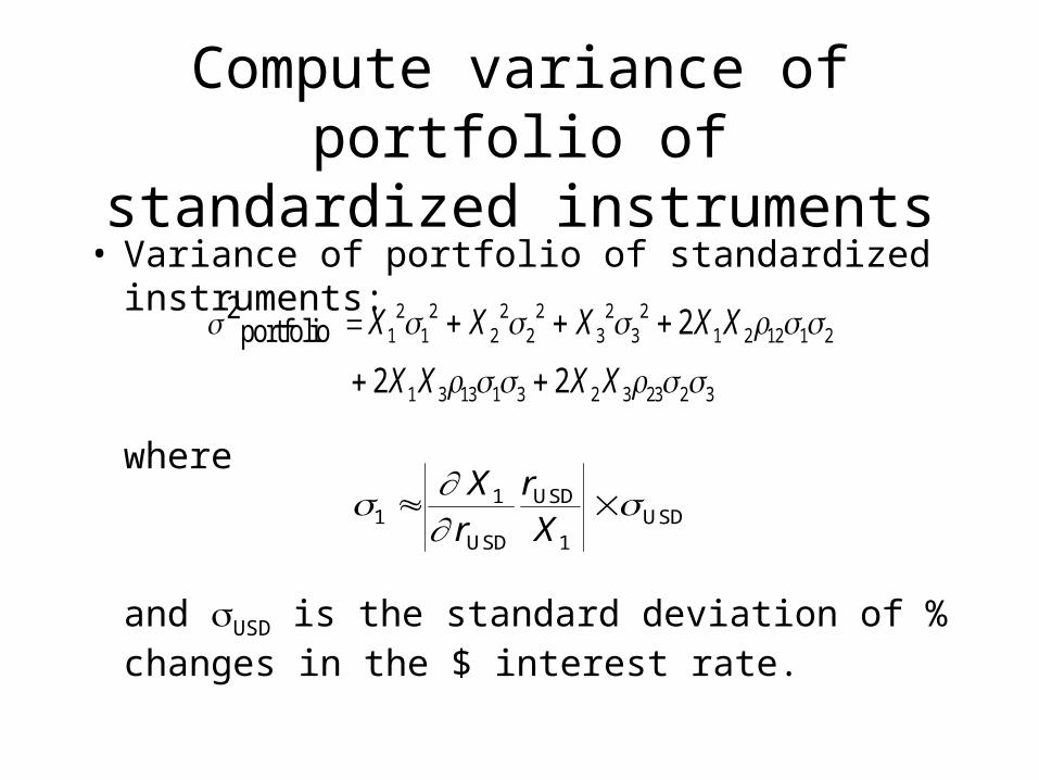
Compute variance of portfolio of standardized instruments
• Variance of portfolio of standardized instruments:
where
and USD is the standard deviation of % changes in the $ interest rate.
21
21
22
22
23
23
21 2 12 1 2
1 3 13 1 3 2 3 23 2 3
2
2 2
portfolio
X X X X X
X X X X
11
1
Xr
rXUSD
USDUSD
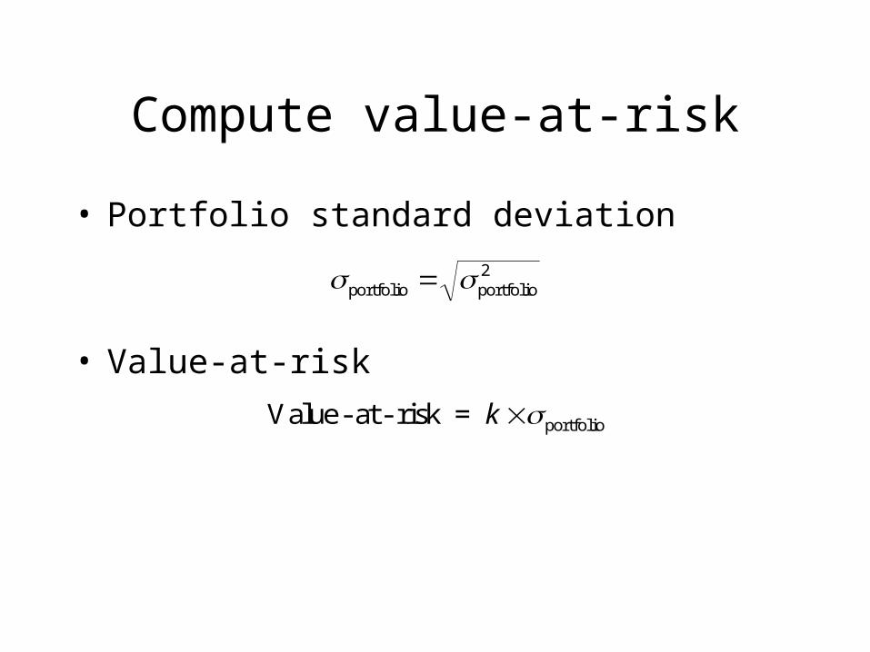
Compute value-at-risk
• Portfolio standard deviation
• Value-at-risk
portfolio portfolio 2
Value - at - risk = portfoliok

Variance-covariance method
value at risk standard deviation of
change in portfolio value
165.
0.0
-150,000 -75,000 0 75,000 150,000
Mark-to-Market Portfolio Profit/Loss
Freq
uenc
y
5% 1.65 std. dev.
Value at risk: $86,625

Monte Carlo simulation
• Like historical simulation• Use psuedo-random changes in the factors rather
than actual past changes• Psuedo-random changes in the factors are drawn
from an assumed multivariate distribution

What Is VaR, Again
• One need not focus on change in portfolio value over the next day, month, or quarter
• Instead, one could estimate the distribution of:– cash flow
– net income
– surplus
– or almost anything else one cares about
• VaR (broadly defined) DFA

Is VaR Appropriate for Property/Liability Insurers?
• Do property/liability insurers have investment portfolios?
• Do they care about the possible future values of things like:– Cash flow?
– Net income?
– Surplus?

What is Value-at-Risk?
0
5
10
15
20
25
P/L
< -
130
-11
0 <
P/L
<-9
0
-70
< P
/L <
-50
-30
< P
/L <
-10
10
< P
/L <
30
50
< P
/L <
70
90
< P
/L <
110
P/L
> 1
30
Hypothetical Daily Mark-to-Market Profit/Loss on Forward Contract (in $thousands)
Fre
quen
cy
value at risk(using x=5%)

Limitations of VaR
• VaR DFA– it is a particular, limited summary of the distribution
• VaR is an estimate of the x percent critical value– based on various assumptions
– sampling variation
• VaR doesn’t indicate what circumstances will lead to the loss– 2 portfolios with opposite interest rate exposure could
have same VaR