RESEARCH ARTICLE

What size is a biologically relevant landscape?

Heather Bird Jackson • Lenore Fahrig

Received: 20 October 2011 / Accepted: 7 May 2012 / Published online: 6 June 2012

� Springer Science+Business Media B.V. 2012

Abstract The spatial extent at which landscape

structure best predicts population response, called

the scale of effect, varies across species. An ability to

predict the scale of effect of a landscape using species

traits would make landscape study design more

efficient and would enable landscape managers to

plan at the appropriate scale. We used an individual

based simulation model to predict how species traits

influence the scale of effect. Specifically, we tested the

effects of dispersal distance, reproductive rate, and

informed movement behavior on the radius at which

percent habitat cover best predicts population abun-

dance in a focal area. Scale of effect for species with

random movement behavior was compared to scale of

effect for species with three (cumulative) levels

of information use during dispersal: habitat based

settlement, conspecific density based settlement, and

gap-avoidance during movement. Consistent with a

common belief among researchers, dispersal distance

had a strong, positive influence on scale of effect. A

general guideline for empiricists is to expect the radius

of a landscape to be 4–9 times the median dispersal

distance or 0.3–0.5 times the maximum dispersal

distance of a species. Informed dispersal led to greater

increases in population size than did increased repro-

ductive rate. Similarly, informed dispersal led to more

strongly decreased scales of effect than did reproduc-

tive rate. Most notably, gap-avoidance resulted in

scales that were 0.2–0.5 times those of non-avoidant

species. This is the first study to generate testable

hypotheses concerning the mechanisms underlying the

scale at which populations respond to the landscape.

Keywords Landscape context � Spatial scale �Habitat fragmentation � Focal patch � Buffer �Informed dispersal �Habitat selection � Edge-mediated

dispersal � Boundary behavior

Introduction

Landscape structure (habitat amount and fragmenta-

tion) has important effects on populations and com-

munities (Laurance et al. 2002; Fahrig 2003), but the

scale at which landscape structure should be measured

is not always clear. A common solution to this

problem is to measure landscape structure within

multiple buffers surrounding a focal patch (Brennan

et al. 2002). Called the scale of effect, the appropriate

scale is the one at which the ecological response (e.g.

abundance) in the focal area is best predicted by

the landscape structure (e.g. habitat amount). This

method ensures that landscape is measured at a scale

Electronic supplementary material The online version ofthis article (doi:10.1007/s10980-012-9757-9) containssupplementary material, which is available to authorized users.

H. B. Jackson (&) � L. Fahrig

Geomatics and Landscape Ecology Laboratory,

Department of Biology, Carleton University, 1125

Colonel Drive, Ottawa, ON K1S 5B6, Canada

e-mail: heather.b.jackson@gmail.com

123

Landscape Ecol (2012) 27:929–941

DOI 10.1007/s10980-012-9757-9

appropriate to the species of interest and has the

benefit of maximizing the probability of finding a

relationship with landscape structure, if one exists.

The disadvantage of this method is that the scale of

effect is discovered after sampling, when it is too late

to use that information to design the study. Empiricists

must therefore sample focal areas far apart to ensure

that landscapes of unknown size are non-overlapping

and independent. If empiricists could accurately

predict the scale of effect beforehand, they could

increase the number of landscapes sampled and reduce

the time and resources spent travelling among focal

areas. Landscape managers, who may not have the

opportunity to empirically derive the scale of effect

before crucial decisions are made, may benefit even

more than empiricists from an ability to accurately

predict the scale of effect.

The scale of effect varies across species (e.g.

Holland et al. 2005a), but which species traits influence

the scale of effect is unknown. Increased body size has

been associated with increased scale of effect for seven

long-horned beetles (Holland et al. 2005a) and four

parasitoid flies (Roland and Taylor 1997), but was not

associated with scale of effect for 56 North American

songbird species (Tittler 2008). Mobility, a correlate

of body size (Bowman et al. 2002; Bowman 2003),

is generally thought to be an important cause for

increased scale of effect (Holling 1992; Carr and

Fahrig 2001; Ricketts et al. 2001; Horner-Devine et al.

2003; Ritchie 2010). This belief is supported by the fact

that other scales of land use that are important to

species, such as home range in mammals (Bowman

et al. 2002) and territory size in birds (Bowman 2003),

are positively related to both dispersal distance and

body size. But the fact that body size is not always

positively related to scale of effect suggests that other

factors besides mobility affect this relationship.

Reproductive rate, which is negatively correlated

with body size (Fagan et al. 2010), may explain some

of the variation in the relationship between body size

and scale of effect. Theory suggests that reproductive

rate can strongly mediate the relationship between

populations and the landscape by allowing populations

to persist with less habitat (Fahrig 2001). Indeed,

reproductive rate is associated with a lower minimum

habitat requirement for birds (Vance et al. 2003) and

wood-boring beetles (Holland et al. 2005b). Untested

is whether an ability to persist with less habitat

translates into a reduced scale of effect.

Informed (i.e. non-random) movement behavior

(Clobert et al. 2009) may also influence the scale of

effect. Whereas many seeds and aquatic larvae

disperse passively, animals often respond to cues to

determine where to settle (e.g. in high quality habitat

or where fewer conspecific competitors are present,

Bowler and Benton 2005). Information use can affect

not only settlement, but also movement (movement is

sometimes referred to as inter-patch movement,

Bowler and Benton 2005, or displacement, Baguette

and Van Dyck 2007). For example, many species are

unlikely to enter unsuitable habitat (matrix), but

instead change direction in order to continue move-

ment within suitable habitat (e.g. Ries and Debinski

2001; Schultz and Crone 2001; Jackson et al. 2009).

The influence of movement behavior on the scale of

effect will most likely result from its influence on the

probability of long-distance dispersal. With an impact

disproportionate to their numbers, rare long-distance

dispersers influence other large scale spatial properties

of populations and species such as the rate of range

expansion (Kot et al. 1996), the spatial patterns of gene

flow (Nichols and Hewitt 1994), and speciation (Guo

and Ge 2005). If instead of settling randomly like a seed,

an animal settles in the first available habitat, then we

expect the distribution of dispersal distances to be

strongly right-skewed (i.e., a ‘‘fat-tailed’’ dispersal

kernel, Turchin 1998), with most individuals settling

close to their natal area but some travelling long

distances to find available habitat. If individuals avoid

high-densities of conspecifics during settlement, then

they are expected to move farther from their natal habitat

on average than if they select habitat without consider-

ing conspecific density. This density-dependent settle-

ment pattern is expected to result in a smaller difference

between maximum and average dispersal distances (a

‘‘thin-tailed’’ dispersal kernel) than habitat settlement

alone (Hawkes 2009) and may reduce the scale of effect.

Gap-avoidance may simply make dispersal distances so

context dependent that a scale of effect measured across

multiple landscapes is hard to identify.

Informed movement behavior may also influence

scale of effect by improving dispersal success. Greater

success at finding breeding habitat would lead to an

increased population growth rate. Gap-avoidance, for

example, was found to be the most important factor

increasing population density when compared with the

effects of increased numbers of patches and reduced

distances between patches in a simulation model

930 Landscape Ecol (2012) 27:929–941

123

(Tischendorf et al. 2005). If increased population

growth rate decreases the scale over which habitat

influences a population, then informed movement

behavior may decrease scale of effect.

We used an individual-based simulation model to

develop quantitative predictions concerning the rela-

tionship between species traits (dispersal distance,

reproductive rate, and movement behavior) and the

scale of effect of habitat amount on abundance. We

tested movement behavior that incorporated increas-

ingly more information: (1) random settlement (RS, in

which individuals settle after a randomly selected

number of steps); (2) habitat-settlement (HS, settlement

in the first territory, i.e. habitat cell, that is encountered);

(3) density-dependent habitat settlement (DHS, settle-

ment in the first territory, i.e. habitat cell, encountered

that is unoccupied by conspecifics); and (4) density-

dependent habitat settlement with gap-avoidance

(DHSG). We expected the scale of effect to be most

strongly associated with average dispersal distance, but

that this relationship would be modified by reproductive

rate and movement behavior.

Methods

Overview

We developed a simulation model (‘‘TraitScape’’)

that simulates dynamics of hypothetical species in

hypothetical landscapes. For a given species type

(characterized by a fully factorial set of species

parameters, Table 1), we conducted multiple simu-

lation runs, each in a different landscape. We then

analyzed the set of runs to determine the scale of

effect of landscape structure on population abun-

dance for that species type. To make our results as

useful as possible for field researchers, we con-

structed the simulations such that the output data

were the same as what would be collected by field

ecologists conducting a ‘‘focal patch’’ landscape-

scale study (Brennan et al. 2002), i.e., where the

response variable (e.g. population abundance) is

measured at the centers of multiple sites and the

predictors are landscape structure variables (e.g.

habitat amount) measured in the landscapes sur-

rounding the focal sites. By conducting multiple

sets of simulations, with different values for the

parameters that determine species type, we tested

the predictions (see ‘‘Introduction’’ section) that

dispersal distance, reproductive rate, and movement

behavior should influence the scale of effect of the

landscape, and we quantified their effects. In

addition, we used information concerning secondary

outcomes (e.g. population size, shape of dispersal

kernel, variation among runs in average dispersal

distances) collected from each treatment combina-

tion to explore the mechanisms linking dispersal

distance, reproductive rate, and movement behavior

to scale of effect.

Table 1 Input parameter values that were experimentally varied

Parameter Experimental treatments Description

Movement step

size (34 levels)aa = 0.1–2.0 by increments

of 0.1, 2–15 by

increments of 1

Step size * Exponential(a)

Reproductive rate (R0) R0 = 1.5, 2.5, 3.5, 4.5 Number of offspring * Poisson(F), where F ¼ R0

1þðR0�1ÞK Na

; K is

carrying capacity of a cell (held constant at 2), and Na is current

number of adults in a cell

Movement behavior

(MOVE) in order of

increasing use of

information

RS Individuals settle when energy reserves are depleted, regardless

of cell type

HS Individuals settle in the first habitat cell encountered or when

energy reserves are depleted, whichever comes first

DHS Same as HS, but individuals do not settle in cells occupied by other

individuals unless energy has been depleted

DHSG Same as DHS, but individuals avoid stepping into matrix

a Median dispersal distance (d50) and maximum dispersal distance (dmax, see Table 3), not step size, are used in analyses of

experimental outcomes, because dispersal distance is the trait most often measured empirically

Landscape Ecol (2012) 27:929–941 931

123

Model description

TraitScape is an individual-based spatially-explicit

model developed using NetLogo (Wilensky 1999).

Freely available online (ccl.northwestern.edu/netlogo),

TraitScape provides abundance in the focal area and

landscape characteristics as output; the scale of effect

must be calculated by the user.

In TraitScape, individuals represent generic mobile

animals and are defined by four state variables:

original position (x0, y0), current position (x, y), age

(0 or 1), and energy level (lifetime number of

movement steps possible). Original position and

energy are determined at birth, current position is

updated after each movement step, and age is updated

once a year.

Simulations are run in a 127 9 127 grid with

reflective boundaries (Table 2; Fig. 1). This grid size

is large enough to allow ten potential scales of effect

(concentric radii from 9 to 63 cells), but small enough to

keep the global population at a computationally man-

ageable size (generally\20,000 individuals). The odd

number of cells (127 9 127) is an artifact of the

midpoint displacement algorithm (Saupe 1988) which is

used to generate naturalistic random landscapes (see

‘‘Submodels’’ section). Grid cell size does not represent

an absolute spatial unit (e.g. meters); instead, the size of

grid cells is only meaningful with respect to the step size

Table 2 Input parameters

which were held constant

for all simulation runs

Parameter Value

Landscape size 16,129 cells (127 9 127)

Length of run The first of the following:

5000 years

when global extinction occurs

when population size varies by less than

10 % between decades for 10 consecutive decades

Spatial autocorrelation of habitat (H) 0.5

Amount of habitat Drawn before landscape setup from Uniform(5, 95 %)

Size of focal area 149 cells (radius = 7)

Initial number of individuals 1,612 (one per 10 cells)

Energy level per individual

(potential number of steps taken

during lifetime)

Drawn at birth from Exponential(9)

Yearly adult mortality 100 % after reproductive season

Movement direction First move: ht¼1�Uniform 0; 2pð Þ for first move

Subsequent moves: ht � ht�1 þ 2 � arctan1�q1þq p½Uniformð�0:5; 0:5Þ�� �

; where q = 0.9

Fig. 1 Examples of randomly generated landscapes used in

TraitScape. Percentages indicate the global habitat amount. Greengrid cells correspond to habitat, and white grid cells are matrix. A

focal area (seven cell radius) at the center of each landscape is

100 % habitat. Concentric circles indicate the radii at which

percent cover of habitat was measured. (Color figure online)

932 Landscape Ecol (2012) 27:929–941

123

of individuals which can vary with user input. Grid cells

are the finest grain at which habitat type is categorized.

Density-dependence in reproduction and settlement

(when applicable) is modeled within grid cells.

Grid cells are classified as either suitable habitat

(hereafter ‘‘habitat’’) or unsuitable habitat (hereafter

‘‘matrix’’). To simplify our model, we did not

explicitly model mortality during movement, whether

in matrix or habitat. All adults die at the end of

reproduction. Therefore, if an individual settles in the

matrix it dies without reproducing. Individuals with

informed movement behavior (Table 1) are respon-

sive to cell type during settlement and/or movement,

and are consequently less likely to settle in matrix.

The model proceeds in time steps, which we call

‘‘years’’ and which are equivalent to generations. In

order to allow populations to stabilize, each run lasts

up to 5,000 years. Most runs are much shorter because

a run is ended when the global population size reaches

a steady state (i.e. if population size varies by less than

10 % from decade to decade for at least 10 decades) or

when the global population goes extinct.

TraitScape simulates the yearly processes of adult

death, juvenile movement (which ends in maturation),

and adult reproduction, in that order (Fig. 2). Each

process is completed before the next process begins.

Within each process, each individual fully completes

its action (e.g. movement) before the next randomly

selected individual initiates action. Within years, time

is not explicitly represented; instead each process

continues until completion and then the next process

immediately begins.

Submodels

Setup An individual simulation run begins by setting

up a random landscape using the midpoint dis-

placement algorithm (Saupe 1988; Figs. 1 and 2).

This algorithm produces realistic-looking landscapes

and allows independent control of the amount of

habitat and the configuration of habitat (for examples

see Saupe 1988; With and King 1999). The algorithm

creates fractal landscapes which can vary in the

amount of spatial autocorrelation according to the

parameter H. The main difference among landscapes

in our runs is the amount of habitat, not the

configuration of habitat. H is held constant at 0.5

(moderate spatial autocorrelation, Table 2), but the

amount of habitat is randomly selected at the

beginning of each run from a uniform distribution

between 5 and 95 %.

Once a random landscape is generated, a focal area

is added to its center. The focal area is the sampling

area within which population abundance is sampled.

To keep local conditions constant among runs, the

focal area is always 100 % habitat. Its radius is seven

cells (Table 2; Fig. 1).

At the beginning of a simulation run, individuals are

placed randomly in the landscape; runs begin with 1,612

individuals (one for every 10 grid cells, Table 2).

Random distribution of individuals without regard for

habitat ensures that the initial density of individuals in

breeding habitat is independent of the amount of habitat

in the landscape (Fahrig 2001). All starting individuals

are juveniles. After initial setup, the model runs on a

yearly time step with three main submodels: adult death,

juvenile movement, and adult reproduction.

Adult death

At the beginning of each year, all adults die (Table 2).

Juvenile movement Movement is modeled one indi-

vidual at a time. Each individual takes successive steps

until settlement occurs. Before each step, an exploratory

loop cycles through possible steps until an acceptable

step (i.e. one in which no forbidden steps are made) is

randomly drawn (Fig. 2). A step outside of the grid

is always forbidden. With DHSG, a step into the matrix

is always forbidden.

Like many animals (Kareiva and Shigesada 1983),

model individuals move according to a correlated

random walk. In a correlated random walk subsequent

movement directions are correlated such that highly

correlated movement paths are nearly straight (Tur-

chin 1998). In the model, the initial direction of

movement for each individual is selected randomly

from between 0 and 2p radians. Thereafter, the

direction of a step is drawn from a wrapped Cauchy

distribution with a mean direction equal to the

previous direction (Table 2, Fletcher 2006). The

concentration around the mean direction is determined

by q, where q = 0 results in a random walk and q = 1

results in a perfectly straight line. For our simulations,

we fixed q at 0.90 (nearly straight) which is close to the

optimal linearity for finding new habitat (Zollner and

Lima 1999; Fletcher 2006; Barton et al. 2009,

Table 2).

Landscape Ecol (2012) 27:929–941 933

123

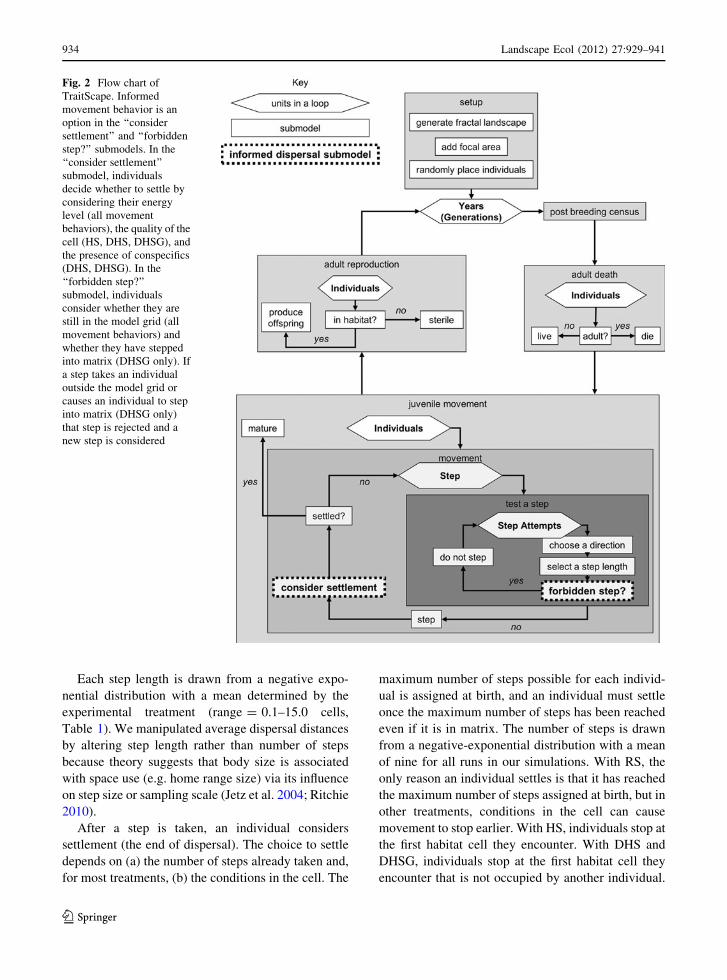
Each step length is drawn from a negative expo-

nential distribution with a mean determined by the

experimental treatment (range = 0.1–15.0 cells,

Table 1). We manipulated average dispersal distances

by altering step length rather than number of steps

because theory suggests that body size is associated

with space use (e.g. home range size) via its influence

on step size or sampling scale (Jetz et al. 2004; Ritchie

2010).

After a step is taken, an individual considers

settlement (the end of dispersal). The choice to settle

depends on (a) the number of steps already taken and,

for most treatments, (b) the conditions in the cell. The

maximum number of steps possible for each individ-

ual is assigned at birth, and an individual must settle

once the maximum number of steps has been reached

even if it is in matrix. The number of steps is drawn

from a negative-exponential distribution with a mean

of nine for all runs in our simulations. With RS, the

only reason an individual settles is that it has reached

the maximum number of steps assigned at birth, but in

other treatments, conditions in the cell can cause

movement to stop earlier. With HS, individuals stop at

the first habitat cell they encounter. With DHS and

DHSG, individuals stop at the first habitat cell they

encounter that is not occupied by another individual.

Fig. 2 Flow chart of

TraitScape. Informed

movement behavior is an

option in the ‘‘consider

settlement’’ and ‘‘forbidden

step?’’ submodels. In the

‘‘consider settlement’’

submodel, individuals

decide whether to settle by

considering their energy

level (all movement

behaviors), the quality of the

cell (HS, DHS, DHSG), and

the presence of conspecifics

(DHS, DHSG). In the

‘‘forbidden step?’’

submodel, individuals

consider whether they are

still in the model grid (all

movement behaviors) and

whether they have stepped

into matrix (DHSG only). If

a step takes an individual

outside the model grid or

causes an individual to step

into matrix (DHSG only)

that step is rejected and a

new step is considered

934 Landscape Ecol (2012) 27:929–941

123

Once an individual has settled, its status is changed

from juvenile to adult and it no longer has the

opportunity to move.

Both step size and number of steps are drawn from

negative exponential distributions to produce nega-

tive-exponentially distributed dispersal distances

(straight-line distance between origin and settle-

ment). A negative-exponential distribution is a com-

mon method used to model ‘‘fat-tailed’’ dispersal, or

more long-distance dispersal than expected under a

Gaussian distribution (e.g. Kot et al. 1996; Chapman

et al. 2007). Fat-tailed dispersal is exhibited by many

species in nature (Okubo 1980; Turchin 1998).

Reproduction If settled in habitat, an adult has the

opportunity to reproduce, with the number of offspring

governed by logistic growth (see also Barton et al.

2009). The number of offspring per individual is

drawn from a Poisson distribution (the distribution

commonly used for simulating stochastic fecundity,

Akcakaya 1991) with a mean determined by

reproductive rate, the carrying capacity for a cell

(k = 2 in our runs), and the density of individuals

within a cell (Table 1).

Simulation experiments

In designing our simulation experiments our goal was

to develop theory that could be used to provide

guidance to empiricists and managers with a rough

estimate of the scale of effect of the landscape on a

given species or species group. The scale of effect, or

the radius at which the relationship between abun-

dance in the focal area and percent habitat cover in the

surrounding landscape is strongest, emerged from

analysis of outputs from Traitscape.

We manipulated (1) step size (in order to influence

dispersal distance), (2) reproductive rate, and (3)

movement behavior in a full-factorial experimental

design (Table 1). Step sizes were selected to ensure

that they spanned the full range of possibilities from an

average dispersal distance of a few cells to an average

distance equal to the width of the grid. One hundred

and fifty runs were conducted for each of the 544

treatment combinations. This provided enough repli-

cates to ensure that a sufficient number of samples

were present after removing those in which extinction

occurred.

Model analysis

Output

Analyses were conducted on data summarized for

each hypothetical species (i.e. each treatment combi-

nation), rather than on raw output of each run (or

landscape). The following raw data were collected

from the last generation of each run (Table 3): the

amount of habitat (As) in each of 10 concentric buffers

around the focal area, median dispersal distance (d50),

maximum dispersal distance (dmax), population size in

the focal area (N), and size of the dispersal kernel tail

(ðdmax � d50Þd�150 ). A dispersal kernel is the full

distribution of dispersal distances in a population.

Measuring the tail (the right side of the dispersal

kernel) indicates how much farther some individuals

move relative to the average disperser. For each set of

runs from the same treatment combination (i.e. with

the same step size, reproductive rate, and movement

behavior, Table 1), raw output from each run was

summarized into primary and secondary outcomes

(Table 3). Primary outcomes included scale of effect

(S*, see below) and the median of both median (d50)

and maximum (dmax) dispersal distances. Secondary

outcomes included median population size (N),

median size of dispersal tails (ðdmax � d50Þd�150 ), and

variation in median dispersal distances (CVd50).

Calculating scale of effect

We evaluated scale of effect using the approach

commonly taken by empiricists (Figure S1, Brennan

et al. 2002), i.e., by selecting the landscape radius at

which habitat cover best predicted abundance in the

focal area. This was done for each treatment combi-

nation (defined by step size, reproductive rate, and

movement behavior, Table 1). Ten linear regression

models were created for each treatment combina-

tion—one for each of the 10 landscape radii (9–63

cells). The landscape radius resulting in the regression

with the lowest AIC value was taken as the scale of

effect (Figure S1, Table 3). Note that the scale of

effect was the same if R2 was used as the selection

criterion (data not shown). The response variable in

each regression was the abundance in the focal area

during the last year (N) and the predictor variable was

habitat amount (As). To ensure that the relationship

Landscape Ecol (2012) 27:929–941 935

123

was linear, only runs with N [ 0 were used in regression

analyses. In addition, we excluded from analysis any

treatment combinations for which the maximum dis-

persal distance (dmax) was greater than the width of the

grid (127 cells) or the median dispersal distance (d50)

was less than one cell. Finally, we deleted treatments

for which scale was unimportant when using habitat

amount to predict abundance. We considered scale of

effect unimportant when the difference in AIC

between the ‘‘best’’ scale and the ‘‘worst’’ scale was

less than 7 (Burnham and Anderson 2002).

Relationship between scale of effect and species traits

We used multiple linear regressions to summarize the

relationships between scale of effect and experimental

treatments (dispersal distance, reproductive rate,

movement behavior). The analysis was performed

twice, once with median dispersal distance used to

summarize dispersal distance and once with maximum

dispersal distance. All two-way interactions were

included in the models. Because of the large sample

sizes available in simulation models, small differences

can yield statistically significant but not necessarily

biologically meaningful results (Zollner and Lima

1999). Thus, instead of focusing on p-values and

F-statistics, we provide the percent sum of squares

(%SS) of predictors to indicate the percent of the

variation explained by independent variables (Fletcher

2006).

That increased dispersal distance will increase the

area over which individuals (and populations) interact

with the landscape is an intuitive concept, but

reproductive rate and movement behavior were

expected to influence scale of effect indirectly through

their influences on secondary outcomes such as

population size, size of the dispersal kernel tail, and

variation in dispersal distances. To understand these

indirect effects we therefore examined the relation-

ships between experimental treatments and these

secondary outcomes, and the relationships between

secondary outcomes and scale of effect, using multiple

linear regression models (Supplementary Material).

Results

As expected, dispersal distance was the strongest

predictor of scale of effect, whether median dispersal

distance (%SS = 46.8 %, Table 4) or maximum dis-

persal distance (%SS = 51.9 %, Table S1) was con-

sidered. Movement behavior was the next most

important predictor and reproductive rate was the

least important (Tables 4 and S1).

Table 3 Model output was collected during the final generation of each run (A). These run-level data were then summarized for each

treatment combination (B, i.e. each ‘‘species’’ or each unique combination of step size, reproductive rate, and movement behavior)

Parameter Description

(A) Output for each run

N Number of adults in the focal area

As Habitat amount (proportion of cells which are habitat) within a circle of radius S cells.

S = 9, 15, 21,…, 63.

d50, dmax Median and maximum dispersal distances of all adults

ðdmax � d50Þd�150

Size of the dispersal kernel tail, standardized by median dispersal distance.

(B) Summary statistics for

each treatment combination

S* Scale of effect which is calculated using the regression of abundance, N, on habitat amount,

As, for each spatial scale, S (Figure S1). S* is the spatial scale (radius) where the

AIC of the regression of N on As is minimized.

d50; dmax Median of median (d50) and maximum (dmax) dispersal distances

N Median number of adults in the focal area (N)

ðdmax � d50Þd�150

Median size of the dispersal kernel tail (ðdmax � d50Þd�150 )

CVd50Coefficient of variation in median dispersal distance (d50), calculated by subtracting

the 2.5th percentile from the 97.5th percentile of all d50 and dividing by d50

936 Landscape Ecol (2012) 27:929–941

123

Scale of effect strongly increased with dispersal

distance (Fig. 3). To report the relationship between

scale of effect and dispersal distance in terms that are

most useful to practitioners, we express the relation-

ship as a ratio. We found this ratio by dividing the

expected scale of effect (i.e. the regression lines in

Fig. 3) by the dispersal distance (median or maximum,

see Figure S2). In most cases (i.e. for medium to large

dispersal distances �d50� 5 cells or �dmax� 50 cells) and

when species were not gap avoidant), the scale of

effect ranged from 3.94 to 8.72 times the median

dispersal distance and 0.28–0.54 times the maximum

dispersal distance (Figs. 3 and S2, Table S2). For

species with short dispersal distances ( �d50\5 cells or�dmax\50 cells), the ratio of scale of effect to median

and maximum dispersal distances was often higher

than for those with longer dispersal distances

(S� �d�150 ¼ 4:50� 18:49; S� �d�1

max ¼ 0:12� 0:74).

Given the same dispersal distance and reproductive

rate, RS, HS, and DHS resulted in similar scales of

effect, but DHSG dramatically reduced the scale of

effect to between 0.19 and 0.47 times the scale found

for other movement behaviors (Figs. 3 and S2, Table

S2). Furthermore, DHSG often resulted in no discern-

ible scale of effect; 73 % of treatments with DHSG

resulted in DAIC B 7 between best and worse scales

(Fig. 4).

The influence of HS on scale of effect was

complicated because the outcome depended on

whether median or maximum dispersal distances were

considered (Figs. 3 and S2, Table S2). Species using

HS had the largest scales of effect when median

dispersal distances were considered; Scales with HS

were 1.07–1.47 times greater than the treatment with

the next greatest scales of effect, RS. Scales of effect

were generally smaller but overlapped with RS (HS

was 0.18–1.02 times RS) and DHS (HS was 0.25–1.29

times DHS) when maximum dispersal distances were

considered.

The remaining differences among groups were

relatively minor (Figs. 3 and S2, Table S2). DHS led

to scales that were barely smaller than scales found for

RS (i.e. DHS was 0.79–0.97 times RS when control-

ling for median dispersal distances). Increased repro-

ductive rate led to slightly decreased scales of effect;

Species with R0 = 4.5 had scales that were 0.63–0.90

times those of species with R0 = 1.5 when controlling

for median dispersal distances.

Movement behavior explained the most variation in

secondary outcomes (Table S3). Informed movement

behavior caused strong increases in population size

(RS \ HS \ DHS \ DHSG), nonlinear variation in

the size of the dispersal kernel tail (RS B DHSG

\ DHS � HS), and increased variation in dispersal

distances (RS \ HS = DHS � DHSG, Figure S3).

Reproductive rate had relatively little impact on

secondary outcomes; its largest association was a

slight positive influence on population size (Figure

S3).

The secondary outcome with the strongest associa-

tion with scale of effect was population size (Figure S4).

Population size had a strong negative association with

scale of effect. The size of the dispersal tail had a

positive association with scale of effect when median

dispersal distance was included in the model, but a

slightly negative association with scale of effect when

maximum dispersal distance was included in the model.

Variation in dispersal distances was weakly to moder-

ately negatively related to scale of effect (Figure S4).

Discussion

Our results support the common belief among

researchers that the scale of effect is primarily a

function of species mobility (Holling 1992; Carr and

Fahrig 2001; Ricketts et al. 2001; Horner-Devine et al.

2003). Importantly, we quantified this relationship,

allowing practitioners to estimate the scale of effect in

Table 4 Results of multiple linear regression of scale of effect

(S*) on median dispersal distance ( �d50), reproductive rate (R0)

and movement behavior (MOVE)

Predictorsa Direction of effect df %SS

�d50 ? 1 46.8

R0 - 3 4.1

MOVE Relative to RS: HS?,

DHS-, DHSG-

3 39.0

�d50: R0 3 0.5

�d50: MOVE 3 4.4

R0: MOVE 9 0.5

R2 (%) 94.2

%SS can be interpreted as the amount of variation explained by

each predictor. These outcomes are similar for a model using�dmax instead of �d50 (Table S1)a Predictors are described in Table 1

Landscape Ecol (2012) 27:929–941 937

123

advance of a study: in most cases landscapes should be

measured at a radius that is 4–9 times the median

dispersal distance or 30–50 % the maximum dispersal

distance of the species of interest. This is the first study

to generate quantitative predictions concerning the

scale at which species respond to landscape structure.

Our study shows the potential for movement

behavior to alter the scale of effect of the landscape.

Most notably, scale is not important when a species

avoids movement in the matrix. The absence of a clear

scale of effect when species were gap-avoidant

probably occurred because gap avoidance caused

dispersal distances to vary widely as a function of

the particular landscape context experienced by indi-

vidual dispersers. For example, dispersal distances of

gap-avoidant species were more strongly influenced

by percent cover than other species (data not shown).

There was an identifiable scale of effect for gap-

avoidant species with large dispersal distances. This

most likely occurred because gaps in habitat were less

likely to be ‘‘noticed’’ by individuals, i.e., individual

steps were more likely to span gaps in habitat. In other

words, increased step size led to a larger ‘‘functional

grain’’ or resolution at which individuals responded to

spatial heterogeneity (Baguette and Van Dyck 2007).

Our data supported the previously unexplored

hypothesis that increased population growth rate can

reduce the scale of effect. Surprisingly, this effect

was more evident with movement behavior treat-

ments than with reproductive rate treatments. Informed

Fig. 3 Relationship between scale of effect (S*, landscape

radius) and movement behavior, reproductive rate (R0), and A

median dispersal distance ( �d50) or B maximum dispersal

distance ( �dmax). Movement behaviors (RS random settlement,

HS habitat settlement, DHS density-dependent habitat

settlement, DHSG density-dependent habitat settlement with

gap-avoidance; see definitions in Table 1) are distinguished by

color and point shape. Plots depict results with increasing

reproductive rate (R0) from left to right. (Color figure online)

938 Landscape Ecol (2012) 27:929–941

123

movement behavior had a much stronger positive

influence on population size than did reproductive

rate, presumably because of lower dispersal mortality

with informed movement. Populations with gap-

avoidance, in particular, were consistently near carry-

ing capacity. A similarly positive effect of gap-

avoidance on population density was found in a

previous model (Tischendorf et al. 2005). In our

model, both gap-avoidance and population size were

associated with a strongly decreased scale of effect,

suggesting that population size (and the underlying

population growth rate that leads to high population

size) may be a strong negative predictor of scale of

effect. Furthermore, the much larger impact of move-

ment behavior relative to reproductive rate on both

population size and the scale of effect emphasizes that

loss of individuals to unsuccessful dispersal can have

major population consequences (e.g. Fahrig 2001).

That high population growth rate is negatively asso-

ciated with scale of effect is a novel prediction and

requires empirical support.

Although a simple description of species’ mobility

(e.g. median or maximum dispersal distance) was

generally a good predictor of scale of effect, more

precise predictions of scale of effect depend on the

variation in dispersal distances within the population

(i.e. the full dispersal kernel). This supports the idea

that single descriptors of dispersal may not always be

adequate, and that variation in dispersal should be

considered (Baguette and Van Dyck 2007; Clobert

et al. 2009). In our model, habitat settlement resulted

in particularly fat-tailed dispersal, such that the

maximum dispersal distance was much longer than

the median dispersal distance. As a result, habitat

settlement was positively associated with scale of

effect when median dispersal distance was held

constant, but was slightly negatively associated with

scale of effect when maximum dispersal distance was

held constant. This means that for a species known to

have fat-tailed dispersal, the scale of effect is near the

high end of the range of possibilities when median

dispersal is considered (*9 times the median dis-

persal distance), but closer to the low end of the range

of possibilities for maximum dispersal distance

(*30 % the maximum dispersal distance).

The scale of effect of some real species will be

affected by multiple species traits simultaneously, as

reflected in our simulations. Density-dependent hab-

itat settlement provides a good example. Density-

dependent habitat settlement resulted in fat-tailed

dispersal kernels relative to RS and also much larger

population sizes. These two secondary outcomes may

have counteracted each other (fat-tails increased the

scale of effect, but large population sizes decreased the

scale of effect), leading to our result that scale of effect

for density-dependent habitat settlement was similar

to the scale of effect for RS given the same dispersal

distances.

We caution that the effects of processes which were

not included in our model should be considered before

important decisions are made. For example, a poten-

tially important influence on scale of effect is

landscape structure itself. In our study, we varied

habitat amount across nearly the entire possible range

(5–95 %), but many species are restricted to land-

scapes with a narrower range of habitat amounts

(10–50 %, for example). Because species’ settlement

and movement is often responsive to landscape

structure, variation in habitat amount can be expected

to alter dispersal distances. Furthermore, habitat

amount has a well-documented positive effect on

population size (Fahrig 2003). Therefore, habitat

Fig. 4 The influence of median dispersal distance, movement

behavior and reproductive rate on the strength of evidence for a

scale of effect (DAIC = AICbest - AICworst). Treatment com-

binations with DAIC \= 7 (the dashed line) showed little

evidence of a distinct scale of effect when describing the

relationship between habitat amount and population abundance.

These treatment combinations were eliminated from analysis.

Movement behaviors (RS random settlement, HS habitat

settlement, DHS density-dependent habitat settlement, DHSGdensity-dependent habitat settlement with gap-avoidance) are

distinguished by color and point shape. Point size indicates

reproductive rate (smallest = 1.5, largest = 4.5). (Color figure

online)

Landscape Ecol (2012) 27:929–941 939

123

amount itself may be a strong influence on scale of

effect. Other variables that might influence the scale of

effect include interspecific interactions and habitat

quality. Both could influence population growth rate

and movement behavior in ways that could alter the

scale of effect.

We offer a few suggestions when using our model

to guide research design and management policy.

First, the predictions from our model are best applied

to the scale of effect of habitat amount because other

aspects of landscape structure (e.g. habitat fragmen-

tation, landscape heterogeneity) may affect a species

most strongly at different scales (Eigenbrod et al.

2008; Smith et al. 2011). Even so, because most

studies indicate that habitat amount will usually have a

greater effect on populations than other measures of

landscape structure (reviewed in Fahrig 2003) our

results provide a quantitative estimate of the most

important scale of effect of the landscape. Second, the

conclusion that scale of effect depends on life history

suggests that habitat evaluation at multiple scales will

be necessary when assessing habitat for species with

disparate dispersal abilities and movement behaviors

(e.g. insects and birds). Third, although we considered

a small, circular sampling area, the scale of effect

should apply to population assessments in large,

irregularly shaped regions as well. If, for example, a

practitioner needs to evaluate the effect of landscape

on a species within an entire park, our model can help

determine what portion of the landscape surrounding a

park should be included in habitat assessments. We

expect land within a buffer as wide as the radius of the

scale of effect surrounding a park to influence a

species of interest within a park.

Acknowledgments We thank Lutz Tischendorf for his

modelling suggestions and for his assistance with NetLogo.

This work was supported by Natural Sciences and Engineering

Research Council of Canada (NSERC) grants to LF. We thank

Nathan Jackson and three anonymous reviewers for their helpful

suggestions.

References

Akcakaya HR (1991) A method for simulating demographic

stochasticity. Ecol Model 54:133–136

Baguette M, Van Dyck H (2007) Landscape connectivity and

animal behavior: functional grain as a key determinant for

dispersal. Landscape Ecol 22:1117–1129

Barton KA, Phillips BL, Morales JM, Travis JMJ (2009) The

evolution of an ‘intelligent’ dispersal strategy: biased,

correlated random walks in patchy landscapes. Oikos 118:

309–319

Bowler DE, Benton TG (2005) Causes and consequences of

animal dispersal strategies: relating individual behaviour to

spatial dynamics. Biol Rev 80:205–225

Bowman J (2003) Is dispersal distance of birds proportional to

territory size? Can J Zool 81:195–202

Bowman J, Jaeger JAG, Fahrig L (2002) Dispersal distance of

mammals proportional to home range size. Ecology 83:

2049–2055

Brennan JM, Bender DJ, Contreras TA, Fahrig L (2002) Focal

patch landscape studies for wildlife management: opti-

mizing sampling effort across scales. In: Liu J, Taylor WW

(eds) Integrating landscape ecology into natural resource

management. Cambridge University Press, Cambridge

Burnham KP, Anderson DR (2002) Model selection and infer-

ence: a practical information-theoretic approach. Springer,

New York

Carr LW, Fahrig L (2001) Effect of road traffic on two

amphibian species of differing vagility. Conserv Biol 15:

1071–1078

Chapman DS, Dytham C, Oxford GS (2007) Modelling popu-

lation redistribution in a leaf beetle: an evaluation of

alternative dispersal functions. J Anim Ecol 76:36–44

Clobert J, Galliard J-FL, Cote J, Meylan S, Massot M (2009)

Informed dispersal, heterogeneity in animal dispersal

syndromes and the dynamics of spatially structured popu-

lations. Ecol Lett 12:197–209

Eigenbrod F, Hecnar SJ, Fahrig L (2008) The relative effects of

road traffic and forest cover on anuran populations. Biol

Conserv 141:35–46

Fagan WF, Lynch HJ, Noon BR (2010) Pitfalls and challenges

of estimating population growth rate from empirical data:

consequences for allometric scaling relations. Oikos 119:

455–464

Fahrig L (2001) How much habitat is enough? Biol Conserv

100:65–74

Fahrig L (2003) Effects of habitat fragmentation on biodiversity.

Annu Rev Ecol Evol Syst 34:487–515

Fletcher RJ (2006) Emergent properties of conspecific attraction

in fragmented landscapes. Am Nat 168:207–219

Guo YL, Ge S (2005) Molecular phylogeny of Oryzeae (Poa-

ceae) based on DNA sequences from chloroplast, mito-

chondrial, and nuclear genomes. Am J Bot 92:1548–1558

Hawkes C (2009) Linking movement behaviour, dispersal and

population processes: is individual variation a key? J Anim

Ecol 78:894–906

Holland JD, Fahrig L, Cappuccino N (2005a) Body size affects

the spatial scale of habitat–beetle interactions. Oikos 110:

101–108

Holland JD, Fahrig L, Cappuccino N (2005b) Fecundity deter-

mines the extinction threshold in a Canadian assemblage of

longhorned beetles (Coleoptera: Cerambycidae). J Insect

Conserv 9:109–119

Holling CS (1992) Cross-scale morphology, geometry, and

dynamics of ecosystems. Ecol Monogr 62:447–502

Horner-Devine MC, Daily GC, Ehrlich PR, Boggs CL (2003)

Countryside biogeography of tropical butterflies. Conserv

Biol 17:168–177

940 Landscape Ecol (2012) 27:929–941

123

Jackson HB, Baum K, Robert T, Cronin JT (2009) Habitat-

specific and edge-mediated dispersal behavior of a sapr-

oxylic insect, Odontotaenius disjunctus Illiger (Coleop-

tera: Passalidae). Environ Entomol 38:1411–1422

Jetz W, Carbone C, Fulford J, Brown JH (2004) The scaling of

animal space use. Science 306:266–268

Kareiva PM, Shigesada N (1983) Analyzing insect movement as

a correlated random-walk. Oecologia 56:234–238

Kot M, Lewis MA, van den Driessche P (1996) Dispersal data

and the spread of invading organisms. Ecology 77:

2027–2042

Laurance WF, Lovejoy TE, Vasconcelos HL, Bruna EM, Did-

ham RK, Stouffer PC, Gascon C, Bierregaard RO, Laurance

SG, Sampaio E (2002) Ecosystem decay of Amazonian

forest fragments: a 22-year investigation. Conserv Biol 16:

605–618

Nichols RA, Hewitt GM (1994) The genetic consequences of

long-distance dispersal during colonization. Heredity 72:

312–317

Okubo A (1980) Diffusion and ecological problems: mathe-

matical models. Springer, New York

Ricketts TH, Daily GC, Ehrlich PR, Fay JP (2001) Countryside

biogeography of moths in a fragmented landscape: biodi-

versity in native and agricultural habitats. Conserv Biol

15:378–388

Ries L, Debinski DM (2001) Butterfly responses to habitat edges

in the highly fragmented prairies of central Iowa. J Anim

Ecol 70:840–852

Ritchie ME (2010) Scale, heterogeneity, and the structure and

diversity of ecological communities. Princeton University

Press, Princeton

Roland J, Taylor PD (1997) Insect parasitoid species respond to

forest structure at different spatial scales. Nature 386:

710–713

Saupe D (1988) Algorithms for random fractals. In: Peitgen

H-O, Saupe D (eds) The science of fractal images.

Springer, New York, pp 71–113

Schultz CB, Crone EE (2001) Edge-mediated dispersal behavior

in a prairie butterfly. Ecology 82:1879–1892

Smith AC, Fahrig L, Francis CM (2011) Landscape size affects

the relative importance of habitat amount, habitat frag-

mentation, and matrix quality on forest birds. Ecography

34:103–113

Tischendorf L, Grez A, Zaviezo T, Fahrig L (2005) Mechanisms

affecting population density in fragmented habitat. Ecol

Soc 10:13

Tittler R (2008) Source–sink dynamics, dispersal, and landscape

effects on North American songbirds. Dissertation, Carle-

ton University, Ottawa

Turchin P (1998) Quantitative analysis of movement: measuring

and modeling population redistribution in animals and

plants. Sinauer Associates, Inc., Sunderland

Vance MD, Fahrig L, Flather CH (2003) Effect of reproductive

rate on minimum habitat requirements of forest-breeding

birds. Ecology 84:2643–2653

Wilensky U (1999) Netlogo. http://ccl.northwestern.edu/net

logo/. Center for Connected Learning and Computer-

Based Modeling, Northwestern University, Evanston

With KA, King AW (1999) Extinction thresholds for species in

fractal landscapes. Conserv Biol 13:314–326

Zollner PA, Lima SL (1999) Search strategies for landscape-

level interpatch movements. Ecology 80:1019–1030

Landscape Ecol (2012) 27:929–941 941

123