When Losses Turn Into Loans:The Cost of Undercapitalized Banks

Job Market Paper

Laura Blattner∗†

Harvard University

Luisa FarinhaBanco de Portugal

Francisca RebeloBanco de Portugal

This version: 31st October 2017

Most recent version

Abstract

We provide evidence that banks hit with a negative shock to capital adequacyinefficiently reallocate credit and that this credit reallocation contributes to themisallocation of capital. A regulatory intervention by the European Banking Au-thority in 2011 provides a natural experiment that unexpectedly increased capitalrequirements for a subset of banks. Using administrative data from the Bank ofPortugal, we show that exposed banks cut back on credit for all but a subset offinancially distressed firms for which banks had been underreporting incurred loanlosses. We argue that the credit allocation to these underreported firms is consistentwith two perverse lending incentives. First, banks roll over loans to distressed firmswith underreported losses to avoid realizing a large loss in case of firm insolvency.Second, undercapitalized banks gamble for the resurrection of distressed borrowersand reduce reported losses to avoid regulatory scrutiny of risky loans. We developa method to back out the underreporting of loan losses using detailed loan-leveldata. We then show that the credit reallocation affects firm-level investment andemployment. A partial equilibrium estimate suggests that the credit reallocationaccounts for close to 20% of the decline in productivity in this period.

∗lblattner@fas.harvard.edu†Laura Blattner thanks Gita Gopinath, Adi Sunderam, Matteo Maggiori, and Jeremy Stein for in-

valuable guidance and support, and Edoardo Acabbi, Juliane Begenau, Gabriel Chodorow-Reich, JohnCoglianese, Karen Dynan, Andrew Garin, Emmanuel Farhi, Jeff Frieden, Xavier Gabaix, Sam Hanson,Eben Lazarus, Pascal Noel, Marcus Opp, Martin Rotemberg, Jesse Schreger, Nicolas Serrano-Velardeand Jann Spiess for helpful comments. The authors thank Manuel Adelino, Antonio Antunes, DianaBonfim, Isabel Correia, Sudipto Karmakar, Gil Nogueira, and seminar participants at the Banco dePortugal. The contribution by Laura Blattner to this paper has been prepared under the LamfalussyFellowship Program sponsored by the European Central Bank. Any views expressed are only those of theauthors and do not necessarily represent the views of the ECB, the Banco de Portugal or the Eurosystem.

1 Introduction

The US government spent over $400 billion to recapitalize US banks as part of its Troubled

Asset Relief Program (TARP) after the 2008 financial crisis. No such program existed in

Europe. As a result, European banks were slow to rebuild capital after the 2008 crisis and

the subsequent sovereign debt crisis. Evidence from another major financial crisis, the

bursting of Japan’s property bubble in the 90s, has led some commentators to conclude

that the absence of a swift bank recapitalization in Europe may have been a costly repeat

of the failure of the Japanese government to recapitalize banks.1

The case for swift bank recapitalization hinges on the claim that undercapitalized

banks make socially inefficient lending decisions which have real economic costs. Existing

research has provided evidence of an empirical link between low capital banks and lending

to failing (‘zombie’) firms but not established causality.2 A separate strand of literature

has suggested that propping up failing firms can have real economic costs but not linked

these costs to the size of the credit distortions.3

This paper uses a novel identification strategy to show that banks hit with a negative

shock to capital adequacy inefficiently reallocate credit and then maps the resulting credit

reallocation shocks into productivity losses. Our identification strategy combines quasi-

experimental variation in banks’ capital requirements with a measure of underreported

loan losses. We argue that the latter serves as a tool to identify firms subject to per-

verse lending incentives. Using detailed firm-level data from Portugal, we show that the

credit reallocation induced by the bank shock affects firm-level investment and employ-

ment. The credit reallocation worsens the misallocation of capital and leads to negative

spillovers for firms unaffected by the credit shock. A partial equilibrium decomposition

of productivity growth suggests that the credit allocation in response to the bank shock

can explain close to 20% of the decline in productivity during this period.

We establish the first link in the causal chain by exploiting quasi-experimental vari-

ation in banks’ capital requirements. The European Banking Authority (EBA) in 2011

unexpectedly announced that a subset of Portuguese banks had to meet substantially

higher capital ratios by mid-2012. Our exposure definition exploits both eligibility, which

was based on a size cut-off, and the severity of the capital shortfall, which was determined

by prior sovereign bond holdings.4 During the period of the EBA intervention only, ex-

posed banks cut lending for all but a subgroup of distressed firms whose loan losses they

had been underreporting prior to the EBA announcement. This effect is estimated in a

1See for example Hoshi and Kashyap (2015).2See Peek and Rosengren (2005), Schivardi et al. (2017) and Acharya et al. (2017)3Caballero et al. (2008), Moreno-Serra et al. (2016)4Defining exposure only based on eligibility would imply that we compare big and small banks. In

addition, this approach would reduce statistical power since not all eligible banks were affected by theEBA exercise. We confirm that both groups of banks, based on our exposure definition, are balanced onobservables, with the exception of size, and that sovereign bond holdings do not follow differential trendsprior to the EBA announcement, which could be correlated with differential trends in credit supply.

1

difference-in-difference design, in which we compare changes in credit from exposed and

non-exposed banks to the same firm. In contrast, exposed banks do not increase credit

to distressed firms that are not underreported prior to the announcement.

A natural explanation for these results is that the EBA intervention heightened two

perverse lending incentives for exposed banks: the delayed recognition of losses and gam-

bling for the resurrection of distressed firms. First, we show that banks had been under-

reporting loan losses with the onset of the European sovereign debt crisis in 2010. While

this underreporting allows banks to boost reported capital and to avoid costly equity

issuance, it also locks banks into a vicious cycle with financially distressed firms whose

losses have not yet been fully accounted for on banks’ financial statements. Cutting lend-

ing to a distressed firm runs the risk of pushing that firm into insolvency which would

force the bank to recognize the previously underreported losses. The capital requirements

imposed by the EBA gave exposed banks an additional reason to avoid capital-reducing

losses and to roll over loans to underreported firms. Consistent with this incentive to de-

lay the recognition of losses, we find that exposed banks sharply increased the amount of

loss underreporting for the duration of the EBA shock. Second, the intervention increased

the incentives of exposed banks to gamble for the resurrection of distressed firms. Banks

correctly anticipated that as long as they made a credible attempt to comply with the

EBA requirements, the Portuguese government would step in at the compliance deadline

to make up any remaining capital shortfall.5 The prospect of the government covering

loan losses increased incentives to lend to risky, distressed firms despite the fact that

these firms were likely to fail. At the same time, banks underreported losses on these

risky firms because underreporting allowed banks to avoid regulatory scrutiny of risky

loans.

We complement the quasi-experimental variation in banks’ capital requirements with

a method to detect the underreporting of loan losses at the firm-bank level. When a firm

falls behind on loan repayments, banks are required to deduct a fraction of the loan as a

loss. In Portugal, the size of this mandatory deduction is tied to the time the firm has

been behind on repayment. Banks can hence reduce loan losses by underreporting the

time a firm has been behind on repayment. We develop an algorithm to back out loss

underreporting from monthly bank reports on the same firm.6 Because the regulatory

deduction schedule features several discrete jumps, the incentive to underreport is largest

just below such a jump (‘bunching’). We conduct several validation tests to show that

underreporting responds to these jumps in the regulatory schedule, thus confirming that

banks strategically report to minimize losses.7

5The IMF and the European Commission had provided a bailout the Portuguese government in early2011. Part of the bailout money was earmarked for the recapitalization of banks.

6Since banks do not provide loan identifiers, we cannot track how long each loan has been overdue inthe data. We hence have to approximate this exercise with a slightly more involved approach.

7Unlike existing work (Diamond and Persson (2016), Dee et al. (2017), Best and Kleven (2016)), wedo not identify bunching based on a cross-sectional distribution over a continuous variable (such as houseprices or test scores) but directly calculate bunching from repeated observations of the same firm-bank

2

Our interpretation of the results rests on the assumption that underreporting is only

correlated with credit allocation through perverse lending incentives. Consistent with

the two types of perverse lending incentives, banks underreport firms that feature larger

losses in the case of insolvency and that display higher levels of risk.8 A potential chal-

lenge is that these firms also happen to have better long-run fundamentals and banks

hence underreport firms where additional lending is socially efficient. In the context our

triple-difference, this would require that banks underreport firms with better long-run

fundamentals, that those firms experience temporary financial distress driving up their

credit demand coinciding exactly with the duration of the EBA intervention, and that

the nature of lending relationships is such that only exposed banks are in a position to

respond to this additional credit demand. To address this possibility, we provide evidence

that underreported firms borrowing from exposed and non-exposed banks do not have

diverging pre-trends in credit or liquidity, that observable measures of firm quality are

not correlated with the borrowing share from exposed banks, and control for relationship

characteristics such as whether the bank is the main lender. More generally, we provide

evidence that underreported firms do not have better long-run outcomes than firms that

are not underreported but are also feature loan losses.

We then show that the credit shock induced by the EBA intervention had real effects

on employment and investment. We first estimate the size of the credit shock at the firm-

level to confirm that firms do not undo the firm-bank level credit effects by substituting

among different lenders. We then estimate the effect of the credit shock on employment

and investment by instrumenting for the firm-level credit change with the firm-level pre-

shock borrowing share from exposed banks. The credit shock has a large and significant

pass-through into employment and investment. An additional euro of credit leads to an

additional 16 cents spent on labor and an additional 40 cents spent on investment. In

addition, we find that the credit shock significantly decreases the likelihood of underre-

ported firms exiting while increasing the likelihood of exit for all other firms. Because the

firm-level credit shocks are large, the effect on investment and employment are sizable. A

simple partial equilibrium calculation implies that underreported firms borrowing entirely

from exposed banks increased employment and investment by 8% and 6% respectively

relative to underreported firms borrowing entirely from non-exposed banks. For all other

firms, the equivalent calculation implies a decline in employment and investment of 9%

and 6%, respectively.

We complete the causal chain by using firm-level data to estimate the effect of credit

reallocation on productivity losses. We decompose total productivity growth into firm-

pair.8Underreported firms have less collateral, which could cover losses in case of firm insolvency, and a

higher share of social security and other debt obligations to the government, which take seniority overany bank debt in Portugal. This is consistent with the incentive of banks to delay the recognition oflosses on their financial statement. Moreover, we find that among firms with loan losses, underreportedfirms have higher sales volatility and higher predicted default risk for all levels of return on equity. Thisfinding is consistent with a gambling motive.

3

level growth rates of output and inputs following Petrin and Levinsohn (2012). This

decomposition allows us to map our cross-sectional firm-level regression results into ag-

gregate productivity growth. Based on these partial equilibrium estimates, the EBA

intervention accounts for over 50% of the decline in aggregate productivity in 2012. This

is driven by the fact that the credit reallocation implies that inputs are reallocated to un-

derreported firms with low factor returns and that the EBA-induced credit crunch reduces

factor use by firms where those factors would have generated a lot of output. A simulation

exercise suggests that keeping the level of credit unchanged but maintaining the credit

reallocation to underreported firms accounts for close to 20% of the productivity decline

in 2012. This result suggests that the credit reallocation matters for productivity losses

above and beyond the effect of the credit crunch. We also show that there are additional

productivity losses from negative spillover effects that underreported firms have on firms

not exposed to EBA banks in the same industry.

The causal chain connecting undercapitalized banks and misallocation applies beyond

the period of the EBA intervention. A novel dataset on new lending operations, which is

only available after the period of the EBA intervention, allows us to identify new loans

that receive a subsidized interest rate via a matching procedure. We show that banks are

more likely to grant new subsidized loans to distressed, underreported firms when they

have a high shadow cost of capital. To establish this result, we use within-bank variation

in the intensity of underreporting as a proxy for the bank’s shadow cost of capital.9

The estimated magnitude is broadly consistent with the quasi-experimental results and

aligns with prior research that shows that loan subsidies are a popular tool to keep failing

borrowers afloat (Caballero et al. (2008)).

An undercapitalized banking sector can also have adverse effects on financial stability:

the underrreporting of loan losses leads banks to overstate their regulatory capital, making

it difficult for the financial regulator to assess the true health of the banking sector. In

particular, we show that the attempt of the EBA to make banks safer had the adverse

consequence of leading banks to substantially increase their underreporting of loan losses

in order to protect regulatory capital. We calculate that without this loss underreporting,

banks would have had to raise additional funds amounting to between 4% and 20% of their

regulatory capital.10 We show that loss underreporting remains elevated after the EBA

intervention and hence continues to reduce capital adequacy in the post-EBA period. To

the extent that European governments provide implicit bailout guarantees to their banks,

these unrecognized losses constitute a hidden fiscal liability for their sovereigns.

Our work is closely related to the literature on ‘zombie’-lending (see Sekine et al.

9We obtain similar but noisier results using a within-bank variation in the proximity to the capitalconstraint

10The range is due the fact that we have to make an assumption about how to calculate the actualtime that an underreported loan has been overdue. The most conservative assumption yields 4%, whileassuming that these loans have been overdue long enough to have been written off completely yields20%.

4

(2003) for a survey on Japan). Existing research has documented that banks close to the

capital constraint tend to give more loans to poorly performing firms, defined by some

observable metric, than banks far away from the capital constraint (Peek and Rosengren

(2005), Schivardi et al. (2017)). Interpreting these results as evidence of perverse lending

incentives is problematic for two reasons. First, distance from the capital constraint

may be correlated with unobserved bank quality. We address this problem by relying

on quasi-experimental variation in capital adequacy. Second, the results may pick up

(efficient) lending to temporarily distressed firms with good fundamentals, or, by failing

to exclude poorly performing firms that are not subject to perverse lending incentives,

underestimate the true effect. We argue that our measure of loss underreporting helps to

address these two challenges because it gives us meaningful variation among distressed

firms11 and we provide evidence that underreporting does not appear to be correlated

with better long-run fundamentals.

Our work ties in the ‘zombie’-lending literature with research on the real effects of

this phenomenon. Caballero et al. (2008) provide a model and related evidence that the

continued existence of zombie firms can have negative spillovers on healthy firms in the

same industry. Moreno-Serra et al. (2016) and Acharya et al. (2017) find similar effects in

Europe by replicating their research design. Schivardi et al. (2017) however find no such

effects in Italy using a slightly amended empirical specification. We both directly map

our credit results into firm-level outcomes and confirm the existence of negative industry-

level spillovers using a quasi-experimental version of the specification in Schivardi et al.

(2017).

We build on a large literature documenting the existence of frictions that distort

the behavior of financial institutions. The first mechanism, which we call delayed loss

recognition, is related to a growing research agenda on how banks manage financial

reporting to improve performance when performance metrics depend on reported figures

(Acharya and Ryan (2016), Falato and Scharfstein (2016)). The lending behavior we

document is similar to gains trading which involves financial institutions selling assets

with high unrealized gains while retaining assets with unrealized losses to boost regulatory

capital (Ellul et al. (2015), Milbradt (2012)). The second mechanism, gambling for

resurrection of distressed borrowers is related to a large literature on “risk shifting” or

“asset substitution” by financial institutions (Jensen and Meckling (1976), Biais and

Casamatta (1999), Acharya and Steffen (2015), Crosignani (2015)).

Our identification strategy follows a growing literature that uses shocks to bank health

to study effects on credit (Chodorow-Reich (2014), Khwaja and Mian (2008)). In partic-

ular, we contribute to a literature that highlights potential unintended consequences of

banking regulation (Behn et al. (2016), Koijen and Yogo (2015)). Gropp et al. (2017) ex-

ploit the same regulatory intervention by the European Banking Authority to show that

banks adjust to higher regulatory capital requirements by cutting back on assets (includ-

11Banks underreport about half of the firms with overdue loans.

5

ing loans) rather than raising equity. While we confirm the finding that banks reduce

credit supply in response to higher minimum capital ratios, our primary contribution lies

in documenting reallocation effects arising from perverse lending incentives.

Finally, we connect a broad literature on banking frictions with a literature on mis-

allocation, which argues that the misallocation of production factors is a key cause of

low productivity and slow economic growth (Restuccia and Rogerson (2008), Hsieh and

Klenow (2009)). A growing number of papers have argued that the presence of financial

frictions at the firm-level is a driver of misallocation (Gopinath et al. (2017), Moll (2014),

and Midrigan and Xu (2014)). We show that bank-level friction can lead to differential

tightening of firm-level financial frictions, thus providing a direct channel through which

banks might contribute to the misallocation of capital.

The remainder of the paper is organized as follows. Section 2 describes our method

for measuring loss underreporting. Section 3 describes the natural experiment, the data

and our results. Section 4 quantifies the effects on aggregate productivity. Section 5

provides evidence on loan subsidies. Section 6 quantifies the effect on capital adequacy.

Section 7 concludes.

2 Loss Underreporting: A Tool to Measure Perverse

Lending Incentives

This section explains why underreporting is correlated with perverse lending incentives

and provides supporting empirical evidence. We provide background on the regulatory en-

vironment that governs the reporting of loan losses in Portugal and describe our method-

ology for backing out underreporting of loan losses. Finally, we provide evidence that our

method produces reliable results by showing that underreporting responds to incentives

present in the regulatory rules.

2.1 Two Sources of Perverse Lending Incentives

We argue that the underreporting of loan losses is correlated with two types of perverse

lending incentives: the delayed recognition of losses and gambling for the resurrection of

distressed borrowers.

Existing research has argued that bank shareholders often resist raising new capital

(Myers and Majluf (1984), Admati et al. (2017)) and prefer to find other ways to improve

regulatory capital ratios, in particular when the bank is already undercapitalized. Since

reported losses deplete a bank’s regulatory capital, banks can protect capital by delaying

the recognition of loan losses. This mechanism is consistent with a growing body of

research that shows how banks manage financial reporting to improve performance when

performance metrics are based on reported numbers (Acharya and Ryan (2016), Falato

6

and Scharfstein (2016)). Since loans constitute the largest assets class for Portuguese

banks, underreporting loan losses is an effective tool to boost regulatory capital.

The underreporting of loan losses locks undercapitalized banks in a vicious cycle with

financially distressed firms whose losses have not yet been fully accounted for on banks’

financial statements. If a bank cuts lending to such a firm, it runs the risk of pushing the

firm into insolvency and having to recognize the entire underreported loss. In contrast,

if the bank rolls over a loan, it avoids the risk of having to mark down the inflated value

of the loan. This extend-and-pretend behavior is similar to gains trading where financial

institutions sell assets with high unrealized gains while retaining assets with unrealized

losses to boost regulatory capital (Ellul et al. (2015), Milbradt (2012)). The incentive to

avoid recognizing a loss to boost regulatory capital leads to the perverse incentive to lend

to distressed firms even when such loans have negative net-present value (NPV). Delayed

loss recognition predicts that banks underreport loans that have large uncovered losses

in the event of firm insolvency, for example loans with little collateral.

The second type of perverse lending incentives arises when undercapitalized banks

gamble for the resurrection of their distressed borrowers. If a bank is sufficiently under-

capitalized that it will default in some states of the world, bank shareholders start to

like gambles. Lending to distressed firms can provide such a gamble if he states of the

world in which those distressed firms go under are also the states of the world in which

the bank itself goes under. In that case, limited liability protects bank shareholders from

losses in these states. Bank shareholders hence only care about states in which distressed

firms recover, which are likely to coincide with the bank remaining solvent. Such “risk

shifting” or “asset substitution” behavior leads banks to invest in negative NPV projects

when these projects have sufficient variance to present a valuable out of the money call

option to bank shareholders (Jensen and Meckling (1976)).12

Banks that gamble for the resurrection of distressed firms also have an incentive to

underreport loan losses on these firms. The Bank of Portugal, which regulated Portuguese

banks at the time, was concerned about risky lending to failing firms in the wake of the

2010-2011 sovereign debt crisis. For example, the Governor of the Bank of Portugal

said in a speech: “The composition of loans granted to non-financial corporations raises

concerns.” And later: “It is crucial that, as deleveraging proceeds, banks continue to

provide an adequate level of financing to the most productive [...] firms in the economy”.13

The main tool used by the regulator to detect risky lending are reported losses. For

example, the Bank of Portugal implemented programs in 2011 and 2012 that inspected a

snapshot of a random sample of bank loans. These inspections would have been able to

flag cases in which banks provided credit to a firm that had already defaulted on a large

12This theory has recently received attention in the context of the European sovereign debt crisis(Acharya and Steffen (2015), Crosignani (2015)).

13Source. http://www.bis.org/review/r140805d.pdf https://www.bis.org/review/r120215c.

pdf

7

part of its loan balance.14 Hence banks had an incentive to reduce reported losses when

engaging in risky lending to avoid regulatory scrutiny. Gambling for resurrection predicts

that underreported firms should be riskier relative to firms that are not underreported

(but also have overdue loans).

2.2 Loss Reporting in Portugal

We exploit the regulatory framework on loan impairment losses in Portugal to measure

the underreporting of loans losses. Once a firm falls behind on loan repayments, the bank

has to deduct a fraction of the book value of the loan as an impairment loss.15 These

deductions are governed by rules set by the financial regulator. Banks deduct impairment

losses as an expense from their income. As a result, impairment losses reduce banks’

regulatory capital by reducing retained earnings. On the balance sheet, impairment

losses mark down the value of the asset.

In Portugal the minimum impairment loss a bank has to deduct depends on the

number of months a loan has been overdue (behind on payments) as well as the type of

collateral (see Figure 1).16 The regulator imposes this mandatory deduction schedule to

force banks to recognize that a full repayment of the loan is less and less likely the longer

a loan has been overdue and to reflect the resulting loss on their financial statements.17

This regulatory setting opens up the possibility of reducing reported losses by man-

aging the reported time a loan has been overdue. Banks are required to report the length

a loan has been overdue, as well as the type of collateral, to the Central Credit Regis-

14While banks were only required to report new lending operations from mid-2012 onwards (partlyinspired by an attempt of the regulator to monitor the quality of loans), auditors and regulators wouldhave been able to infer a new loan by comparing residual and origination maturity in their snapshot ofloans. They would not have been able to infer any underreporting for which they would have needed thepanel data we exploit in this paper.

15We use the term overdue as a synonym for a borrower being behind on payments. A loan is non-performing if the borrower is more than 90 days behind on repayments. A borrower can have overdueloans which are not yet non-performing if the payments are overdue for less than 90 days. We use defaultand overdue as synonyms.

16These rules are set out in Banco de Portugal instruction 3/95. 3/95 was in place before the inter-national accounting standards IAS39, which also contain rules on impairment losses, became binding inPortugal. The Portuguese regulator refers to impairment losses under 3/95 as loan loss provisions but weuse the term impairment losses for ease of exposition. Since the Portuguese financial regulator preferredthe more stringent existing framework, banks have to deduct the difference between impairment lossesunder 3/95 and IAS39 from their regulatory capital. This means that 3/95 is the effectively bindingregulation with regards to impairment losses in Portugal. 3/95 applies on an individual basis to allbanks (regardless of whether they follow the standard approach or the internal-rating based approachunder the Basel regulatory framework). On a consolidated basis, banks do not have to comply with 3/95but impairment losses deducted at the individual basis will still negatively affect regulatory capital onthe consolidated basis through retained earnings.

17In principle, a bank should deduct the full difference between the carrying amount of the asset(shown on the balance sheet) and the expected discounted cash flow (at the origination interest rate) asan impairment loss. However, impairment losses above the regulatory minimum are not tax-deductible inPortugal and hence Portuguese banks generally do not exceed the minimum deduction required (Dermineand de Carvalho (2008)).

8

Figure 1: Regulatory Rules on Loss Deductions

110

2550

7510

0M

anda

tory

pro

visi

onin

g (%

)

0-23-5

6-89-11

12-1415-17

18-2324-29

30-35

Time overdue (months)

No collateral GuaranteeReal collateral

Notes. The graph shows the regulatory rules that govern mandatory minimum deductions for loan lossesbased on the number of months a loan has been overdue, and the type of collateral.

ter (Central de Responsabilidades de Credito) at a monthly frequency.18 Banks report

the time overdue in discrete intervals, or buckets, which correspond to the regulatory

buckets shown in Figure 1. We exploit this detailed reporting in order to measure loss

underreporting.

We focus on firm finance loans granted to non-financial firms. Firm-finance loans

tend to have longer maturities than some other credit products, such as credit cards, and

therefore are better suited for detecting loss underreporting which requires us to track

a lending relationship over time. Firm-finance loans constitute the main loan product

for firms and capture about 36% of the banks’ corporate loan portfolio. However, since

the vast majority of firms have at least one firm-finance loan with each of their lenders,

we capture almost the entire population of bank-dependent firms in Portugal. Table 5

in Appendix B presents descriptive statistics on the loans that we use to measure the

underreporting of loan losses. 73% of loans are collateralized and 67% have origination

maturity above a year.

2.3 A Method to Detect Underreporting of Loan Losses

Our aim is to measure to what extent banks underreport loan losses by managing the

reported time a loan has been overdue. Unfortunately, we cannot simply compare re-

ported time overdue to the actual time overdue in the data since banks do not provide

identifiers to track loans over time. Instead, we develop an algorithm to measure the

18Banks start reporting this variable in 2009.

9

extent of underreporting in each reporting bucket for all firm-bank pairs at a monthly

frequency.19

Algorithm We now illustrate the basic version of the algorithm. We denote the

observed loan balance reported in overdue bucket k in month t by Bib(t; k) where i

denotes the firm and b the bank. We drop the firm-bank subscripts in the discussion that

follows. There are 14 reporting buckets which correspond to the overdue buckets in the

regulatory schedule: k ∈ {{0} , {1} , {2} , {3, 4, 5} , . . . , {30, . . . , 35}}.

Table 1: Example of Loss Underreporting

Overdue Performing Excess<30 days 1 month 2 months credit mass

2012m1 EUR 50 EUR 450 0

2012m2 EUR 50 EUR 450 0

2012m3 EUR 50 EUR 450 50

2012m4 EUR 50 EUR 450 0

Notes. The table shows a stylized example of the loan data collapsed to the monthly firm-bank level. Weshow lending volumes of a hypothetical firm-bank pair. We show the first three reporting categories ofhow long a loan has been overdue. Performing credit denotes the balance of loans in the firm-bank pairwhich are not (yet) overdue. Panel A shows an example where the bank does not update the reportedtime overdue in March, which is registered as excess mass by the algorithm (mechanism 1). The excessmass column shows the excess mass as calculated by the formula given in the text. The last rows in eachexample illustrate that the algorithm is “memory-less”: As long as reporting is consistent relative to theprevious month, the algorithm does not register excess mass.

The goal of the algorithm is to measure excess mass, a term we borrow from the

bunching literature (Diamond and Persson (2016), Dee et al. (2017) or Best and Kleven

(2016)). We define excess mass in an overdue bucket k in month t, E(t; k), as the lending

balance that is reported in a bucket k that exceeds the lending balance we would have

expected to observe in bucket k based on the amount observed at t − 1. For the first

three reporting categories, which consist of a single month, excess mass is defined as

E(t; k) = B(t; k)−B(t− 1; k − 1) (1)

Intuitively, the loan balance we observe in bucket k at t must be the loan balance that

has moved up from the preceding bucket in the previous period. We define excess mass

19Our set-up differs from the standard bunching setting where the researcher observes a continuousvariable, such as house prices or test scores. In those settings, bunching can be measured based onexcess mass in the observed cross-sectional distribution at points of particular importance, such as testscore cut-offs (Diamond and Persson (2016), Dee et al. (2017) or Best and Kleven (2016)). In our set-up, we instead calculate excess mass from repeated observations of the same firm-bank unit and detectdiscrepancies in observed reporting for the same firm-bank pair over time. In contrast to the standardsetting, we also have to address the challenge that reported time is not continuous but discretized.

10

as the deviation from this identity. For reporting buckets that consist of several months,

we have to adjust this simple formula and introduce an auxiliary step, which is described

in Appendix A.

Table 1 provides a stylized example of the loan data, a monthly firm-bank panel, with

the overdue loan balance reported separately for each bucket. The third row of Table 1

shows an example where the bank does not update the reported time overdue, thereby

underreporting how the long has been overdue. Banks use three mechanisms to adjust

the reported time overdue: (a) they don’t update the reported time, (b) they average new

overdue loan installments with the time overdue on the existing overdue loan balance, and

(c) they grant new performing credit in exchange for the repayment of an overdue portion

of the loan. In Appendix A we provide stylized examples of the second and third type of

behavior and show that most underreporting is driven by these two types of behavior.

The algorithm is Markovian and only records inconsistencies relative to t−1. That is,

it does not keep a tally of how far the reporting has fallen behind the ‘true’ time overdue.

In Appendix A, we provide evidence from a subset of single-loan relationships, where we

can track the ‘true’ time overdue and show that the gap between reported and true time

widens over time (Figure 6a in Appendix B). This suggests that the algorithm returns a

lower bound of the underreporting of loan losses.

For ease of exposition, the version of the algorithm outlined here does not take into

account flows in the data. Flows consist of additional loan installments falling overdue,

loan repayments or loan restructuring and write-offs. In Appendix A, we describe the full

version which incorporates inflows and outflows in the data. Appendix A also describes

extensive robustness checks.20 We run the full version of the algorithm on the set of

non-performing corporate firm-finance lending relationships in 2009-2016.

There are two actions that banks can take to reduce reported loan losses that are not

captured by the algorithm. First, banks can swap out all overdue credit for performing

credit. This action will not be captured by the algorithm since there is no more overdue

lending reported. Second, banks could prevent a firm from falling overdue in the first

place by granting loans that allow the firm to stay current on loan repayments.

Validity Checks Given that the regulatory deduction schedule features several dis-

crete jumps, we would expect banks to do most of their reporting management in re-

porting buckets just before a jump (‘bunching’). We test whether underreporting in

fact occurs in buckets just before a jump. Such responsiveness of bank behavior at the

micro-level is evidence that our measure is indeed picking up strategic behavior.21

Figure 2 illustrates the intuition of our first validity test. We plot the distribution of

20We show that we can bound the effect of flows by calculating excess mass for the set of most restrictiveand most permissive assumptions respectively. We show that the bounds are narrow since credit flowsare quantitatively small relative to credit stocks.

21The algorithm does not restrict excess mass to be zero even when there is no increase in the regulatoryrate in the next higher reporting bucket.

11

Figure 2: Underreported Losses by Reporting Category

515

25Ra

te in

crem

ent (

p.p.

)

0.2

.4.6

Und

erre

port

ing/

loan

s

0-23-5

6-89-11

12-1415-17

18-2324-29

30-36

Reporting bucket (months)

UnderreportingIncrement in regulatory rate

(a) Bunching Test

515

25Ra

te in

crem

ent (

p.p.

)

0.2

.4.6

Und

erre

port

ing/

loan

s

0-23-5

6-89-11

12-1415-17

18-2324-29

30-36

Reporting bucket (months)

UnderreportingIncrement in regulatory rate

(b) Placebo test

Notes. The graphs show the amount of loss underreporting scaled by the overdue loan balance byreporting bucket. We show averages across all firm-bank pairs for loans without collateral. The verticallines denote increments in the regulatory impairment deduction rate from one reporting category tothe next for loans without collateral. A dot at zero means that the rate remains constant between twobuckets. The right panel show the rate increments for loans with collateral and illustrates the logic ofthe Placebo test described in detail in section 2 and the results of which are reported in table 3

underreported losses across reporting categories for all firm-bank pairs. We pick loans

that have no collateral as an example. Panel a provides suggestive evidence that the

amount of underreporting respond to the increments in the regulatory deduction rate,

which we plot as vertical lines. We can formally test this responsiveness by regressing the

amount of underreporting in a reporting category on the size of the rate increment in the

next higher category. We run this regression separately for each type of collateral since

the regulatory rules differ by collateral type. We describe the regression specification in

detail in Appendix A.

The regression confirms that for each type of collateral the amount of underreporting

is statistically significantly higher when there is an increase in the regulatory rate in the

next higher bucket relative to buckets where the regulatory rate stays constant (see Table

3 in Appendix A). Moreover, we find that underreporting is higher if the increment in

regulatory deduction rate is higher, suggesting that underreporting responds not only

the location of the jumps in the regulatory rate but also to the size of the increment.

There is one exception where this monotonicity fails: the largest increment for loans with

either real collateral or borrower guarantees, which does not feature more underreporting

relative to the second-largest increment. This non-monotonicity arises because loans

in the reporting category just below the second-largest jump have to be declared non-

performing, which has additional negative effects beyond increasing the impairment loss.

Non-performing loan ratios are a closely watched indicator of bank health by both the

regulator and financial markets giving banks a reason to concentrate their underreporting

in lower reporting buckets.

Panel b of Figure 2 shows a natural placebo test. If we regress underreported losses

12

on the regulatory increments of another collateral type, we should not find positive and

significant coefficients in categories where only the other collateral type features an a jump

in the deduction rate. Table 3 in Appendix B shows that we find negative coefficients for

all three collateral types, suggesting that there is significantly less underreporting when

only other collateral types feature an increase in the regulatory rate.

In Appendix A, we provide an additional validity check which is based on the sample

of single-loan relationships, where we can directly trace the time a loan has been overdue.

As expected, we find that underreporting is most pronounced in the months when the

regulatory rates increases.

2.3.1 Underreporting as a Tool to Measure Perverse Lending Incentives

Underreporting of loan losses is a powerful tool to identify lending driven by perverse

incentives. Banks only underreport about half of firms with overdue loans and this un-

derreporting is very persistent, giving us meaningful variation among firms with overdue

loans (see Figure 3 and Figure 6b in Appendix B).22 By relying on our measure of un-

derreported losses, we overcome the challenge that perverse lending incentives do not

necessarily apply to all firms that exhibit observable signs of financial distress or poor

performance. This avoids the attenuation bias in measures of ‘zombie’ lending in the

existing literature.

Figure 3: Prevalence of Loss Underreporting

0.2

.4.6

.8Fr

actio

n of

rela

tions

hips

2009m1 2011m7 2014m1 2016m7

Underreported loss Overdue

(a) Fraction of Relationships

.1.2

.3.4

.5O

verd

ue lo

ans/

loan

vol

ume

0.0

2.0

4.0

6U

nder

repo

rted

loss

/loan

vol

ume

2009m1 2011m7 2014m1 2016m7

Underreported loss Overdue

(b) Share of Loan Volume

Notes. Panel a shows the fraction of firm finance lending relationships that have a some overdue loansand the fraction of relationships that are subject to loss underreporting as measured by the our algorithm.Panel b shows the overdue balance scaled by total loan volume (RHS), and the amount of underreportedlosses scaled by total loan volume (LHS).

We also show that the predictions of the two sources of perverse lending incentives

22A variance decomposition confirms that most variation in underreporting is driven by within-firmrather than by between-firm variation. To obtain this decomposition, we regress the amount of underre-porting on a firm, bank, time and relationship fixed effect.

13

are borne out in the data. Table 5 in Appendix B shows that, among firms with overdue

loans, underreported firms have statistically significant lower collateral values, hold more

assets and a higher share of social security and other debt obligations to the government,

which take seniority over any bank debt in Portugal. This is in line with the prediction

that delaying losses is most important in lending relationships that have large uncovered

losses in the case of firm insolvency.

In line with the risk-shifting mechanism, we find that underreported firms display

higher levels of risk for all levels of profitability relative to firms that have overdue loans

but are not underreported. Panels a and b of Figure 4 plot firm-level risk measures (sales

volatility and predicted default risk based on firm observables) against firm-level return

on equity, residualized on year, industry, firm age, district and size.

Figure 4: Correlation of Underreporting with Firm-Level Risk

.7.8

.91

Sd(lo

g sa

les)

0 .2 .4 .6 .8 1Return on equity

Not underreportedUnderreported

(a) Volatility of Sales

.06

.08

.1.1

2D

efau

lt ris

k

0 .2 .4 .6 .8 1Return on equity

Not underreportedUnderreported

(b) Predicted Default Risk

Notes. The graphs show a residualized binned scatter plot of firm-level risk measures against the returnon equity. The left panel uses the standard deviation of firm-level sales across 2005-2015. The rightpanel uses default risk based on the Bank of Portugal’s internal credit risk prediction model that usesfirm-level observables. The sample only includes firms with overdue loans. We compare firms that areunderreported to firms that are not underreported. The correlations are residualized on firm age, year,district, industry and firm size.

We now address two potential shortcomings of using underreporting to identify per-

verse lending incentives. First, our measure of loss underreporting only applies to firms

that already have some overdue loans. However, in the time period we study a large

number of firms fell behind on payments (see Figure 3 in Appendix B), implying that we

capture a large fraction of lending in the economy. Moreover, perverse lending incentives

are most likely to arise for firms that are already close to financial distress and likely to

have already defaulted on a loan payment.

Another potential challenge is that underreporting may be correlated with unobserved

firm-quality differences and banks may exploit soft information to underreport firms where

continued lending is positive net present value. This would imply that underreporting

does not capture banks inefficiently lending to failing firms but banks efficiently lending

to firms likely to recover. While our empirical specification, outlined in the next section,

14

relies on comparing changes in credit to the same (underreported) firm, it is still helpful

to address this point more generally.

First, underreported firms show signs of severe financial distress. These firms are

highly levered, have little cash, and exhibit low profitability and sales growth. Based on

these observables, underreported firms do not look like firms that are likely to recover

soon. We provide additional evidence in the next section that these signs of financial

distress do not appear to be driven by temporary negative shocks, at least in the period

we study. We also show there are no evidence that underreported firms have significantly

better fundamentals than their non-underreported peers (see Table 5 in Appendix B).

Second, we compare long-run outcomes for underreported and non-underreported

firms. In Figure 7 in Appendix B, we plot the path of exit, sales, return on assets

and the fraction of loans overdue from the year in which the firm first has overdue loans.

The variables are residualized on year×industry and firm size fixed effects. We show that

the trends are similar for the group of firms whose losses are underreported and those

that are never underreported (but have overdue loans). While ex-post outcomes are not

the same as banks’ ex-ante expectations, it is unlikely that banks would consistently

overpredict the long-run outcomes of firm that they choose to underreport.

3 The Cost of Undercapitalized Banks: A Natural

Experiment

This section first describes the regulatory intervention by the European Banking Author-

ity which we exploit for identification. We briefly describe our data and then present our

main results.

3.1 The 2011 EBA Special Capital Enhancement Exercise

In October 2011, the European Banking Authority (EBA)23 announced a Special Capital

Enhancement Exercise to force banks with large, or overvalued, sovereign debt exposures

to improve their capital ratios by June 2012. The EBA intervention applied to the

largest banks in each country based on a cut-off determined by the EBA.24 The EBA

announcement was plausibly unexpected given that banks had already undergone a round

of EBA stress tests in June 2011. The Financial Times in 2011 reports that the EBA

requirements were “well beyond the current expectations of banks and analysts”. The

intervention led to a large capital shortfall for most eligible Portuguese banking groups

since their Eurozone sovereign debt holdings were substantial and often valued above

23The EBA is an EU agency tasked with harmonizing banking supervision in the EU.24Banks covered by the EBA exercise had to jointly hold at least 50% of the national banking sector

as of the end of 2010 (EBA 2011).

15

market prices in their balance sheets.25

Affected banks anticipated that as long as they made a credible attempt to comply

with the EBA requirements, the Portuguese government would step in to make up any

remaining capital shortfall at the compliance deadline. In May 2011, the Portuguese gov-

ernment had received a financial assistance package from the IMF and European Finan-

cial Stability Facility, which explicitly earmarked EUR 12 bn to recapitalize Portuguese

banks.26 As a result, the EBA announcement sparked expectations that banks would tap

into the bailout fund to comply with the requirements. For example, Bloomberg reported:

“A possible outcome is Portuguese banks have to tap the bailout fund, said Andre Ro-

drigues, an analyst at Caixa Banco de Investimento SA in Lisbon.” These expectations

were validated when in June 2012, at the EBA compliance deadline, the Portuguese gov-

ernment provided EUR 6 bn of capital in the form of convertible contingent bonds. All

banks with large capital shortfalls due to the EBA exercise received a government bailout

in June 2012, which allowed them to comply with the EBA requirements.

We define a bank as exposed to the EBA intervention if it belongs to a banking

group that was both subject to the intervention and had a large capital shortfall. We

exploit variation in eligibility and variation in the EBA capital shortfall. The shortfall

was driven by both quantity and valuation of banks’ sovereign bond holdings. We use the

variation in the shortfall to address the size imbalance that stems from the EBA targeting

only the largest banks. Our control group hence consists of banks that were subject to

the EBA intervention but had a small capital shortfall and also any commercial bank

operating in Portugal not subject to the EBA intervention. We exclude any bank whose

foreign parent was subject to the EBA intervention in another European country. Using

variation in pre-announcement sovereign debt holdings is valid as long these holdings

are not correlated with other bank-level trends that affect credit allocation. Figure 5a

shows that sovereign bond holdings followed parallel trends among the two groups prior

to the EBA announcement providing evidence consistent with this assumption. Table

2 shows that both groups of banks are balanced on observables prior to the shock with

the exception of size, which is to be expected given the selection criteria of the EBA

intervention.

The EBA intervention temporarily heightened two sources of perverse incentives driv-

ing inefficient lending for exposed banks. First, exposed banks, which were already low

on regulatory capital prior to the EBA intervention, wanted to comply with the higher

capital ratios but do so without raising costly new capital. Hence exposed banks had an

incentive to boost reported capital by increasing the intensity of their loan loss underre-

25In Portugal four banking groups (containing 7 banks) were subject to the Capital Exercise. Bankshad to achieve a minimum Core Tier 1 ratio of 9% including an additional ‘sovereign buffer’, whichreflected capital needs due to sovereign debt holdings.

26The European Commission report on the Assistance Programme says: “The financing needs for theProgramme’s financial sector strategy primarily consist of a contingency provision to support strongerbanking sector capitalization” (Commission 2011). see p. 16 of http://ec.europa.eu/economy_

finance/publications/occasional_paper/2011/pdf/ocp79_en.pdf

16

Figure 5: Comparing Behavior of Exposed and Non-exposed Banks19

2021

2223

log(

Euro

zone

sov

erei

gn d

ebt)

2005q1 2007q3 2010q1 2012q3 2015q1

Exposed Non-exposed

(a) Evolution of Sovereign Debt Holdings

0.0

5.1

.15

Und

erre

port

ing/

2010

cap

ital

2009m4 2010m8 2011m12 2013m4 2014m8

Exposed Non-Exposed

(b) Evolution of Underreported Losses

Notes. Panel a shows the aggregate log Eurozone sovereign debt holdings of banks exposed and notexposed to the EBA Special Capital Enhancement exercise. The vertical line denotes the announcementof the EBA exercise. Panel b shows the evolution of aggregate underreported losses for the two groupsof banks. Underreported losses are scaled by 2010 bank capital. The first vertical line denotes theannouncement of the EBA intervention. The second vertical line denotes the EBA compliance deadline.

porting and simultaneously rolling over loans to underreported firms. Figure 5b shows

that underreporting at exposed and non-exposed banks follows the same increasing trend

with the onset of the crisis but shoots up for exposed banks with the announcement of

the EBA intervention. This increase lasts until the EBA deadline, at which point exposed

banks roll back the additional underreporting. Banks had an incentive to complement

this underreporting with rolling over loans to firms with underreported losses. Doing

so allowed banks to avoid realizing a large loss in case of firm insolvency. Second, the

prospect of a government bailout gave bank shareholders the incentive to gamble for the

resurrection of distressed borrowers. The bailout was effectively a government guarantee

to cover any loss in June 2012. From the shareholders perspective, distressed firms would

either recover allowing them to satisfy the constraint without the government’s help, or

they would fail but the resulting losses would be borne by the government.

3.2 Data

We use proprietary administrative data from the Portuguese central bank. We combine

quarterly bank balance sheet data with information from the EBA website to determine

which banks were eligible for the exercise either directly, or through a foreign parent, as

well as the capital shortfall due to the EBA intervention. We merge the bank informa-

tion with the credit register data (Central de Responsabilidades de Credito), a loan level

database, which covers the universe of lending relationships that exceed EUR 50. We

collapse the loan data to the quarterly firm-bank level. We then merge this information

with balance sheet and other financial variables for non-financial firms. The data comes

17

from the Simplified Corporate Information (Informacao Empresarial Simplificada), an

annual, mandatory firm census.

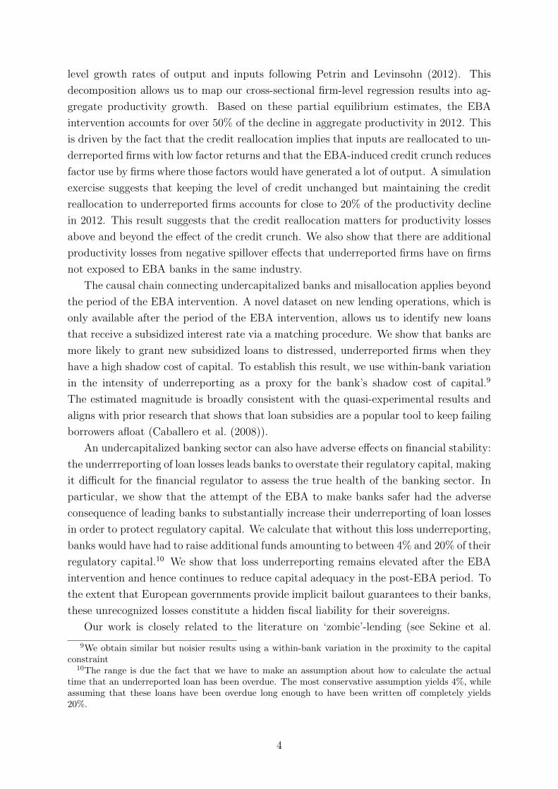
We work with three final datasets. First, a quarterly dataset of loan balances at

the firm-bank level from 2009-2015 spanning 45 banks, 144,050 non-financial firms, and

380,286 relationships. The dataset covers over 90% of loans made in Portugal. Second,

we collapse the firm-bank data to a quarterly firm-level dataset covering the same time

period and number of firms. Third, we use the annual firm-level information from 2009-

2015. We drop firms with fewer than 2 employees or missing information (or negative

values) on assets or employees in 2008-2011. The firms in our resulting sample cover 81%

of sales and 73% of assets in Portugal. We winsorize all outcome variables at the 1% level

separately for each 2-digit industry.

Table 2: Descriptive Statistics: Firms and Banks

Firms BanksBaseline Not exposed Exposed Dif

Assets (m) 1.62 Assets (100 bn) 0.42 0.98 0.56∗∗∗

(6.05) (0.32) (0.34) (0.21)Employees 13.46 Sovereign bonds 0.04 0.06 0.02

(114.14) (0.04) (0.02) (0.01)Total credit (m) 0.52 Loans 0.46 0.49 0.03

(4.86) (0.14) (0.11) (0.06)Share NPLs 0.07 NPLs 0.02 0.02 0.00

(0.22) (0.02) (0.01) (0.00)Return on assets 0.03 Return on assets 0.00 0.00 0.00

(0.07) (0.02) (0.00) (0.00)Sales growth 0.13 Deposits 0.33 0.40 0.07

(0.48) (0.17) (0.13) (0.07)Leverage 0.28 Capital ratio 0.10 0.14 0.04

(0.73) (0.14) (0.02) (0.03)Current ratio 2.43 Liquid assets 0.01 0.01 0.00

(4.29) (0.01) (0.00) (0.00)Cash/assets 0.13 Central bank funding 0.12 0.09 -0.03

(0.17) (0.11) (0.06) (0.04)Fixed assets/assets 0.47 Interbank market 0.22 0.13 -0.09

(0.29) (0.20) (0.11) (0.06)N 144,050 38 7

Notes. The table shows descriptive statistics for firms and banks in our sample. All variables aremeasured at the end of 2010. We only include firms in our sample (firms that report consistently to theannual firm census in our sample period in 2008-2011). All bank variables with exception of assets arescaled by total assets. Exposed refers to banks that are exposed to the EBA intervention. Dif refers tothe difference in means for exposed and non-exposed banks. ** indicate significance at the 0.05 level.

3.3 Results

Banks subject to the EBA intervention cut credit for all but the subset of financially

distressed firms whose loan losses they had been underreporting prior to the EBA in-

tervention. This credit reallocation is present both at the firm-bank level, controlling

18

for the total change in firm-level credit, and at the firm-level. We show that there is a

substantial pass-through of the credit shock into employment and investment spending.

3.3.1 Credit Effects at the Firm-Bank Level

We run the following difference-in-differences specification at the firm-bank level

gcreditibt =

5∑τ=−2

βtreatτ (periodτ × exposedb) +5∑

τ=−2

βperiodτ τ (period× underreportedib)

+5∑

τ=−2

βtreatgroupτ (periodτ × underreportedib × exposedb) + θit + ϕb (2)

+βbase1 (underreportedib × exposedb) + βbase2 underreportedib + α2Xibt + εibt

where i, b and t index firms, banks and quarters respectively.27 The main explanatory

variables are exposedb, a dummy variable that is 1 for banks exposed to the EBA interven-

tion and underreportib, a dummy that is 1 if the lending relationship has underreported

loan losses in the four quarters prior to the announcement of the shock. This dummy is

based on our measure of underreporting.

periodτ is a dummy that indexes periods of three quarters. The periods of interest are

the EBA shock (2011Q4-2012Q2) and the period following the EBA deadline (and bank

bailout) (2012Q3-2013Q1). We also include two pre-period dummies and one post-bailout

period dummy, all of which are of equal length.28

ϕb is a bank fixed effect and Xibt are relationship level controls.29 Standard errors are

two-way clustered at the firm and bank level.30 We follow the literature and estimate

the effect on changes rather than (log) levels. The growth rate of credit is our dependent

variable: yibt = creditt/creditt−1 − 1. The growth rate allows us to decompose the total

change in credit into the portion coming from overdue credit and the portion coming

from performing credit (credit that is not overdue).

The firm×quarter fixed effects, θit, control for the firm-level changes in credit growth.

This implies that we compare changes in the share of credit coming from exposed and

non-exposed bank to the same firm (Khwaja and Mian (2008)). This estimator requires

27We condition on relationships that are present throughout the entire period of interest. In a separatespecification we investigate the effect on the probability that a lending relationship is cut.

28The two pre-periods allow us to test for pre-trends in credit allocation, while the inclusion of thepost-bailout period allows us to study the evolution of credit following the EBA deadline. The sampleperiod includes 2009Q1-2014Q4 which allows us to estimate each βτ . This implies that the quarters notcontained in any of the period dummies are the omitted base group. A standard difference-in-differenceswould omit the t-2 and t-1 terms and include only a single post coefficient which would summarize theaverage treatment effect in the post period.

29The relationship controls are the lending share of the bank, the length of the relationship, a dummyif the bank is the main lender, the share of the firm in the bank’s loan portfolio

30We also run a version with standard errors only clustered at the bank-level.

19

firms to have multiple lending relationships, which is true for 56% of firms in our sample.

We also run a model with separate firm and quarter fixed effects which then also includes

firms that only have a single lending relationship.

The coefficients of interest are βtreatgroupτ on the triple interaction, which estimate

the treatment effects for the subset of underreported firms. Our hypothesis is that the

EBA intervention increased perverse lending incentives for exposed banks and we expect

this coefficient to be positive during the EBA intervention. Given that the differential

incentives disappear with the government bailout, we expect βtreatgroupτ to either turn to

zero (or negative) following the EBA deadline.

We also estimate the baseline treatment effects for all other firms, βtreatτ for two

reasons. First, the existing literature suggests that a tightening of capital requirements

can lead banks to shed assets and decrease credit supply (Admati et al. (2017), Gropp

et al. (2017)). We want to test whether the effect is present in this setting. Second,

the total treatment effect for the subset of interest, firms with underreported losses, is

βtreatτ +βtreatgroupτ . We need to estimate the baseline treatment effect in order to calculate

the full treatment effect on the subset of underreported firms.

Results Figure 6a shows our main credit results (see also Table 7 in Appendix B for

corresponding point estimates). Following the announcement of the EBA intervention,

exposed banks increase credit supply to firms in financial distress that are subject to prior

loss underreporting. The coefficient on the triple interaction of periodτ×underreportedib×exposedb in equation 2 is positive and strongly significant during the EBA intervention.

This positive treatment effect for underreported distressed firms contrasts with the credit

crunch for all other lending relationships at exposed banks. The coefficient on EBAt ×exposedt in equation 2 is negative and statistically significant (Figure 6a and columns 2

and 3 of Table 7). The magnitude of the shock is large. The baseline treatment effect

of borrowing from exposed banks is a 2 percentage point (p.p.) drop in quarterly credit

growth between the announcement and deadline of the EBA intervention. In contrast,

the treatment effect for underreported, distressed firms is an increase in credit growth at

exposed banks of just over 2 p.p.31 These changes are equivalent to 4% of a standard

deviation of credit growth.

If loss underreporting correctly identifies firms for which perverse lending incentives

drive additional lending, we should find that exposed banks do not increase credit supply

to firms that are distressed but are not subject to underreporting. In Figure 6b, we

show results from running specification 2 but replacing the triple interaction with the

subgroup of firms that have overdue loans but are not subject to underreporting prior to

the shock. We find no evidence of differential treatment effects for these relationships at

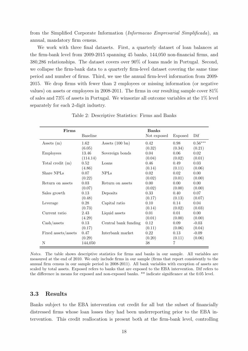
the intensive margin and a small positive treatment effect at the extensive margin.32

31The total treatment effect adds the baseline treatment effect and the treatment effect for the subgroupof underreported firms.

32See also Table 6 in Appendix B

20

Figure 6: Firm-bank Credit Results-.0

6-.0

30

.03

.06

Trea

tmen

t effe

ct

2010Q2-Q42011Q1-Q3

EBABailout

2013Q2-Q4

All others Underreported

(a) Underreported firms

-.06

-.03

0.0

3.0

6Tr

eatm

ent e

ffect

2010Q2-Q42011Q1-Q3

EBABailout

2013Q2-Q4

All others Not underreported

(b) Non-underreported firms

Notes. The graphs shows results of the firm-bank level credit regression in specification 2, whichincludes firm×time and bank fixed effects as well as firm-bank-level controls. The dependent variableis the quarterly credit growth.. We plot the coefficients on the two interactions periodτ × exposedb andperiodτ × underreportedib × exposedb, which are the respective treatment effects for the baseline groupof firms and the group of firms subject to loss underreporting. In panel b, we plot the triple interactionperiodτ × not underreportedib × exposedb, which are relationships with loan losses but which are notunderreported. Standard errors are clustered at the firm and bank level. The shaded area marks theperiod of the EBA intervention. See Table 7 in Appendix B for point estimates. N = 1,981,219.

The results suggest that effects are indeed driven by changes in bank credit supply in

response to the EBA intervention. There is no evidence of differential credit allocation

at exposed banks in the two periods prior to the shock, lending credibility to our parallel

trends assumption. The lack of pre-trends applies to both the baseline group of firms

and to the subgroup of underreported, distressed firms. Second, the preferential credit

treatment for underreported, distressed firms only occurs during the period of the EBA

shock when exposed banks face heightened perverse lending incentives. Similarly, the

credit crunch only occurs in the period of the EBA shock when banks attempt to comply

with tighter capital requirements. We provide a series of further robustness checks in

Table 8 in Appendix B.33

While the differential treatment effect in growth rates disappears with the EBA dead-

line, the effect is persistent in levels. That is, we do not find evidence of negative treatment

effects for underreported, distressed firms in the periods after the EBA shock. This sug-

gests that banks do not withdraw the additional credit granted during the EBA shock

following the EBA deadline.

The effect on changes in total credit is almost entirely driven by performing credit

(column 4 of Table 7 in Appendix B). If underreported, distressed firms were simply

converting more of their performing loan balances into overdue loans, we would expect

33We show that the estimated treatment effects are robust to the inclusion of firm-level controlsaveraged over the pre-period and interacted with period dummies. We also show that the estimatedtreatment effects are robust to differential clustering of standard errors, exclusion of relationship controls,and a weighted least squares specification.

21

no change in total credit, a reduction in performing credit, and an increase in overdue

credit. Instead, we find an increase in total credit, an increase in performing credit, and

a (statistically insignificant) reduction in overdue credit.

There are similar patterns when looking at the probability that a bank grants a

new loan. We construct a dummy that is one if there is a new loan in a firm-bank

relationship.34 Column 6 of Table 7 in Appendix B shows that we find a large significant

increase in the probability that a new loan is granted to a underreported, distressed firms

at exposed banks in the period of the EBA shock. In contrast, the probability declines

for all other firms at exposed banks.

The differential credit behavior is also visible at the extensive margin. The probability

that an exposed bank cuts a relationship increases by almost 6 percentage points during

the EBA shock (Table 9 in Appendix B ).35 Crucially, this probability falls by 16 per-

centage points for underreported, distressed firms. These results suggest that banks fully

insulate underreported, distressed firms from the negative effect of the credit crunch.36

3.3.2 Credit Effects at the Firm-Level

To detect whether firms undo effects at the firm-bank level by adjusting their credit

coming from non-exposed banks, we analyze changes in credit allocation at the firm-

level. We run the following fully dynamic differences-in-differences specification37

∆ log creditit =10∑

t=−5

δtreatgroupt (quartert × treatmenti × underreportedi) (3)

+10∑

t=−5

δtreatmentt (quartert × treatmenti) + controls + α1Xit + θi + εit

34Our definition of a new loan requires that the total number of loans in a firm-bank relationshipsincreases and that the total loan balance in the firm-bank relationships increases. While the creditregister data does not allow us to track individual loans, banks report each individual lending operationto a given firm allowing us to count the number of loans each period. Since existing loans can be splitinto several loans due to for example a restructuring operation we also impose the second condition onthe total loan balance.

35Our indicator is a dummy that turns one in the month the performing credit balance drops tozero. We focus on the performing credit stock since banks often report relationships that only havenon-performing credit to the credit register for a very long time even when the credit is fully writtenoff. The reason is that banks wait for the conclusion of the official insolvency process to stop reportingthe debt to the credit register. Given very lengthy bankruptcy procedures in Portugal, this implies thatnon-performing loan stocks can be reported in the credit register for years even though there no longerexists a meaningful credit relationship.

36We cannot estimate pre-trends in this specification since we condition on the sample of relationshipswith positive loan balances in the pre-period. Since we estimate the cumulative effect of existing alending relationship, the dummy for exit remains 1 following the quarter of exit and contributes to theestimated probability in all subsequent quarter, the changes in the coefficients are informative about theadditional exit. This implies that as in intensive margin, the effects predominantly take place during theEBA shock.

37see for example Jager (2016) and Jaravel et al. (2015)).

22

where treatmenti is the firm-level borrowing share from exposed banks prior to the

shock.38 We standardize this variable to be able to interpret coefficients as the per-

centage change in credit in response to a standard deviation increase in the borrowing

share from exposed banks.39 underreportedi is a dummy that captures firms with under-

reported losses prior to the announcement of the shock. Standard errors are clustered at

the firm-level.

In contrast to the firm-bank level specification, we can no longer control for the firm-

level change in total credit, which captures changes in credit demand. We therefore

include a range of firm-level controls interacted with quarter dummies to allow for flex-

ible differences in time trends across firms. These controls include 2-digit industry and

several firm characteristics averaged over 2008-2010 (sales growth, capital/assets, inter-

est paid/ebitda and the current ratio). The inclusion of controls accounts for potential

long-term trends at the firm-level that could affect credit demand.

Results Figure 7a shows our main credit results at the firm-level. Following the an-

nouncement of the EBA intervention, underreported firms with a larger borrowing share

from exposed banks experience a faster growth in credit than underreported firms with

a smaller borrowing share from exposed banks. A the same time, credit declines for all

other firms with a larger borrowing share from exposed banks. Both effects shift back to

zero following the bank bailout at the EBA deadline. We hence confirm that the credit

reallocation at the firm-bank level is also present at the firm-level, suggesting that firms

cannot undo the effects at the firm-bank level.

Unlike in the firm-bank results, the treatment effect for underreported firms does not

immediately revert after the bank bailout at the EBA deadline. This persistent effect on

total credit is driven by an increase in overdue credit which begins after the EBA deadline

(see Figure 9a in Appendix B). This result suggests that banks can stave off additional

overdue loans for underreported firms in the short-run but eventually their default rates

catch up. This result, together with the absence of pre-trends at the firm-level, provides

further support for the argument that the credit reallocation is not driven by underlying

differences in firm-level quality or liquidity trends. The increase in credit during the EBA

intervention is again driven by performing credit as shown in Figure 7b.

The economic significance of the credit reallocation is large. For underreported, dis-

tressed firms, the total treatment effect of borrowing exclusively from exposed banks

versus borrowing exclusively from non-exposed banks is equal to a 16% increase in total

credit relative to the base quarter (2011Q3).40 For all other firms, the total treatment

38Following (Chodorow-Reich (2014)) this is defined as treati =∑Bexp

b=1 Lib,pre∑Ball

b=1 Lib,pre

where Lib,pre denotes

the stock of total credit of firm i at bank b in 2010. Bexp is the set of exposed banks, while Ball is theset of exposed and non-exposed banks.

39Figure 5 in Appendix B shows that we have variation in treatment intensity.40This is the cumulative effect over the combined EBA and bailout period, which runs from 2011Q3

to 2013Q1. A standard deviation in the borrowing share in our sample is the equivalent of borrowing

23

Figure 7: Firm-level Credit Treatment Effects-.1

-.05

0.0

5.1

Trea

tmen

t effe

ct

2011Q12011Q3

2012Q12012Q3

2013Q12013Q3

All others Underreported

(a) Total Credit

-.1-.0

50

.05

.1Tr

eatm

ent e

ffect

2011Q12011Q3

2012Q12012Q3

2013Q12013Q3

All others Underreported

(b) Performing Credit

Notes. The graphs show results of the firm-level credit regression in specification 3. The dependentvariable is the quarterly log of total credit for a given firm in panel a and the quarterly log of performingcredit in panel b. We plot the coefficients on the two interactions quartert × treatmenti and quartert ×treatmenti × underreportedi, which are the treatment effects for the baseline group of firms, and thegroup of firms subject to loss underreporting. The shaded area marks the period of the EBA intervention.The specification includes the full set of interactions, industry×quarter and firm fixed effects, as wellas firm-level controls interacted with quarter. All coefficients should be interpreted as changes in thedependent variable relative to the (normalized) base quarter 2011Q3. Standard errors are clustered atthe firm-level. N= 1,346,771.

effect is a decline in credit of 14% relative to the base quarter.

3.3.3 Pass-Through into Employment and Investment

We use an instrumental variable design to estimate the pass-through of the credit shocks

into employment and investment at the annual firm-level.

yis = γ∆ log creditis + controls + uis (4)

where i and s index firms and industries respectively.

We instrument for ∆ log creditis with the firm-level borrowing share from banks ex-

posed to the EBA shock. We include the same controls as in the firm-level credit speci-

fication, equation 3. To address concerns that treated firms may have been on different

long-term trends, we include a lag of the dependent variable.

The dependent variable is either the symmetric growth rate of employees, wages and

fixed assets, or investment spending scaled by lagged fixed assets. The symmetric growth

rate is a second-order approximation of the log difference growth rate around zero (Davis

et al. (1996), Chodorow-Reich (2014)). This growth rate is attractive since it takes into

entirely from exposed and borrowing entirely from non-exposed. For underreported firms, this is thetotal treatment effect βtreatτ + βtreatgroupτ in equation 3, or in other words, we add the two coefficientsdisplayed in Figure 7a.

24

account observations that turn to zero and is bounded between -2 and 2.41 Because the

employment effect combines extensive and intensive margin changes, we run a separate

specification isolating the intensive margin effects. Growth rates are calculated between

2011 and 2012 since we expect real outcomes to be affected in 2012 as this is when most

of the EBA intervention occurs.

Results We estimate that the credit shock has a 40% pass-through into investment42

and a 11% pass-through into employment (see Table 3). If we allow for the effect of exit,

the pass-through into employment jumps to 60%. The first-stage F-statistics are close to

200, comfortably above the Stock and Yogo (2005) criterion for 5% maximal bias.

Table 3: Pass-Through Into Employment and Investment

Growth rate (1) (2) (3) (4) (5) (6)Employees Wages CAPEX Fixed assets

OLS Ext + int Intensive∆ log crediti 0.082*** 0.596*** 0.109*** 0.160*** 0.391** 0.353***

[0.004] [0.084] [0.025] [0.033] [0.138] [0.109]Lag -0.041 -0.011 0.152*** 0.129***

[0.035] [0.010] [0.018] [0.034]Controls N Y Y Y N YIndustry, size FE Y Y Y Y N YN 156,784 156,784 119,563 119,563 13,431 119,563First-stage F statistic 200 176 176 3 176

Notes. The table shows IV regression results at the annual firm-level for 2012. The dependent variablein columns 1-2 is the symmetric growth rate of employment, which is a second order approximation tothe log difference growth rate and incorporates observations than turn to 0 (firm exit). In the remainingcolumns, we condition on the sample of firms that do not exit (intensive margin). Column 5 estimates theeffect on CAPEX scaled by lagged fixed assets. Given that only larger firms report CAPEX, this resultshould be treated with caution (weak instrument). With the exception of column 1, we instrument for thelog change in credit using the (normalized) firm-level borrowing share from banks exposed to the EBAintervention. Controls consist of firm-size and 2-digit industry FE, as well as firm-level log total assets,interest/ebitda, capital/assets, currrent ratio, cash/assets and sales growth all averaged over 2008-2010.Lag refers to the lag of the dependent variable. Standard errors are clustered by industry. Standarderrors in parentheses. *, **, and *** indicate significance at the 0.1, 0.05 and 0.01 level.

The real effects of the EBA intervention persist into 2013 but dissipate in 2014 (see

Table 10 in Appendix B). However, it is difficult to precisely estimate the long-run pass-

through since the credit shock is short-lived and hence the instrument loses power after

41The formula is

gyi,s =yt + yt−1

0.5(yt + yt−1)

42While the firm census asks for CAPEX, in reality only large firms provide CAPEX numbers. Asa result our instrument loses power because we have a much smaller sample and credit shocks tend tobe less important for the largest firms. We instead resort to the growth rate in fixed assets to measureinvestment. Table 3 reports results for using CAPEX scaled by lagged fixed assets and shows that weobtain similar results despite a weak instrument problem (F-statistic of 3).

25

2012. For additional robustness, we show that results are similar when dropping firm-

level controls and the lagged dependent variable (see Table ?? in Appendix B). We also

conduct placebo exercises running the same specification in the years prior to the shock

and find no significant effects (see Table 10 in Appendix B).

A partial equilibrium back-of-the-envelope calculation that combines the firm-level

credit estimates with the pass-through coefficients is suggestive of the magnitude of the

real effects. In 2012, underreported firms borrowing entirely from exposed banks increased

employment and investment by 8% and 6% respectively relative to underreported firms

borrowing entirely for non-exposed banks.43 For all other firms, the equivalent calcula-

tion implies a decline in employment and investment of 9% and 6%, respectively. This

partial equilibrium calculation abstracts from any general equilibrium effects of the EBA

intervention.

3.3.4 Potential Threats to Identification

The validity of our results rests on the assumption that the credit reallocation to under-

reported firms by exposed banks is not driven by credit demand. For this assumption to

be violated in the context of our triple-difference design, banks have to underreport firms

with better long-run fundamentals, those firms have to experience temporary financial

distress driving up their credit needs coinciding exactly with the duration of the EBA in-

tervention, and the nature of lending relationships has to be such that only exposed banks

are in a position to respond to these additional credit needs. To address this possibility,

we first provide evidence that observable characteristics of underreported firms are not

systematically correlated with how much they borrow from exposed banks prior to the

EBA intervention (see Figure 8a). Turning to the firm-bank level, Figure 8b shows that

EBA banks are no more likely to be the main lender, to grant a different level of credit,

or to have a different share of performing credit. EBA banks seem to have slightly longer

lending relationships and on average firms account for a larger share in the EBA banks’

loan portfolio. These differences are likely to reflect that exposed banks on average are

larger and have been present in Portugal for longer. To account for these differences, we

control for relationship characteristics in all firm-bank level specifications.

Second, we investigate the potential presence of differential financial shocks driving

outcomes. Given that we absorb any firm-level changes by firm×time fixed effects in

our main specification, differential shocks to credit demand provide a potential challenge

only for our firm-level regressions. At the firm-level, the main difficulty for confounding

firm-level financial shocks to explain the results stems from the fact that the EBA inter-

vention is temporary. For concurrent liquidity shocks to explain the results, we would

43A standard deviation in the borrowing share in our sample is the equivalent of borrowing entirely fromexposed and borrowing entirely from non-exposed. We can multiply the firm-level coefficient from thefirst-stage credit regression with the pass-through coefficient (0.14*0.353 for investment and 0.14*0.596for employment.

26

need that firms borrowing from exposed banks experience a negative liquidity shock, lead-

ing to a positive credit demand shock, at the time of the EBA intervention and that this

shock dissipates with the onset of the EBA deadline. Nonetheless, we provide evidence

against different liquidity trends prior to the shock by estimating a dynamic firm-level

difference-in-differences regression at the annual level with liquidity ratios as the depen-

dent variable. Figures 8a - 8b show that there are no pre-trends in either the current ratio

or the cash/assets ratio for these firms. Figure 8c plots firm×quarter fixed effects from a

regression that decomposes credit change of firms with multiple lending relationships into

a bank and a firm-time component. The firm×quarter fixed effects can be interpreted

as a measure of firm-level credit demand. There is no evidence of differential trends in

credit demand prior to the EBA intervention.

Figure 8: Correlations with Borrowing Share from Exposed Banks

assets

employees

sales gr

roa

leverage

current ratio

cash/assets

fix/assets

-.08 -.04 0 .04 .08Correlation (95% CI)

(a) Firm-level

loan size

share performing

rel length

firm share

main lender

bank share

-.08 -.04 0 .04 .08 .12Correlation (95% CI)

(b) Relationship-level

Notes. Panel a shows the correlation of normalized firm-level observables with the (normalized) firm-leveltreatment variable for the subset of firms subject to loss underreporting. Treatment is the borrowingshare from banks exposed to the EBA intervention. The correlations are conditional on 2-digit industryfixed effects and firm size buckets. All variables are averaged over 2008-2010. The right panel showsthe correlation of normalized relationship-level variables with a bank exposure dummy for the subset ofrelationships subject to loss underreporting. share performing refers to the share of total credit that isnot in default. rel length refers to relationship length. firm share refers to the share of the firm’s loanbalance in the bank’s loan portfolio. main lender is a dummy if the bank is the firm’s largest lender.bank share refers to the share of the bank in the firm’s loan portfolio.

One remaining potential issue is that underreported firms may be aware of their

special status and also aware of the EBA shock affecting their lender. Firms could use

the shock to extract additional credit from the bank by threatening immediate default on

outstanding payments, which would impose a loss on the bank at a time when bank capital

is scarce. According on anecdotal evidence, firms are passive actors in banks’ reporting

management and likely unaware of whether or not they are underreported. However, even

if this mechanism were in operation, it would be consistent with the inefficient lending

channel that this paper documents.

27

4 Measuring the Effect on Misallocation and Pro-

ductivity

A growing literature has documented that distortions that affect the allocation of produc-

tion factors across firms are a key cause of low productivity (see Restuccia and Rogerson

(2017) and Hopenhayn (2014) for recent surveys). Perverse lending incentives by under-

capitalized banks can drive such factor misallocation in two ways.

First, when banks reallocate credit from non-distressed firms to distressed, under-

reported firms, they prevent labor and capital held by underreported firms from being

reallocated to firms where those factors would have potentially earned higher returns. At

the same time, credit taken up by underreported firms shrinks the available credit supply

for firms with potentially high factor returns forcing them to shed labor and capital. This

channel is consistent with a growing body of research that points to firm-level financial

frictions as a driver of factor misallocation (Gopinath et al. (2017), Moll (2014), and

Midrigan and Xu (2014)). We provide evidence that these firm-level financial constraints

can in turn be caused by frictions at the bank-level.

Second, firms that are not affected by the EBA shock may still be affected by the con-

tinued presence of distressed, underreported firms. For example Caballero et al. (2008)

provide evidence from Japan that a higher share of near-insolvent firms (‘zombies’) re-

duces the profits for healthy firms in the same industry, which discourages entry and

investment of healthy firms. Such congestion effects act like a tax on healthy firms caus-

ing them to hire less labor and capital than they would have done in the absence of the

zombie firms.

We follow the popular approach of inferring the presence of distortions, which give

rise to factor misallocation, by measuring wedges in firms’ first-order conditions (Restuc-

cia and Rogerson (2008), Hsieh and Klenow (2009)). We use a decomposition due to

Petrin and Levinsohn (2012), which is more amenable to aggregating firm-level changes.

We conduct two partial equilibrium counterfactual exercises to measure the impact on

productivity arising from each of the two channels.

4.1 Decomposing Productivity Growth

We compute the contribution of reallocation to aggregate productivity growth using a

decomposition due to Petrin and Levinsohn (2012). This decomposition is based on an

economy with N firms, each of which produces a single good with a production technology

Qi(Ai, Xi), where Ai and Xi denote firm-level technical efficiency and inputs. Production

uses two primary inputs, capital and labor, and two intermediate inputs, materials and

services. Together these make up the input vector Xi.44

44The choice of services as an intermediate is a bit unorthodox but the Portuguese firm data does notprovide information on electricity use, which is frequently used as an intermediate use. Instead the datahas high quality information on services used in the production process.

28

The portion of firm i’s output which is not used as an intermediate input at other

firms goes into final demand Yi:

Yi = Qi −∑

x∈M,S

inputxi. (5)

where M and S index materials and services.

We define aggregate productivity growth (APG) as the difference between the change

in the value of final output and the change in the costs of primary inputs (all deflated).

APG ≡∑i

PidYi −∑i

∑x∈K,L

Wxidinputxi (6)

where Wxi denote input prices and K and L index capital and labor.45

By totally differentiating output, aggregate productivity growth can be decomposed

into the change in firm-level physical productivity, or technical efficiency, Ai and the

reallocation of inputs across firms.

APG =N∑i=1

Did logAi︸ ︷︷ ︸Technical efficiency

−N∑i=1

Di

∑x∈K,L,M,S

(εxi − sxi) d log inputxi︸ ︷︷ ︸Reallocation of inputs

(7)

where Di = PiQi∑i V Ai

is a Domar weight46, sxi = WxiinputxiPiQi

is revenue share of input x, and

εxi is the output elasticity with respect to to input x.

In the absence of any frictions and distortions, firm profit maximization implies that

the revenue share of an input equals the output elasticity (εxi = sxi). In this friction-

less benchmark, all firms equate marginal products and the reallocation term would be

zero. Hence there would be no productivity gains from reallocating an input across firms

because an input earns the same marginal product at each firm. However, in practice

many real-world features lead to input gaps, sometimes to referred to as wedges (see for

example Hsieh and Klenow (2009)). To the extent that gaps are driven by distortions

such as financial constraints, taxes, or market failures, re-allocating inputs to firms with

high gaps increases aggregate productivity. In turn, anything that leads inputs the be

allocated away from high gap firms and towards low gap firms reduces productivity and

therefore output.

45This expression is in terms of final demand, which already incorporates the effect of changes inintermediate inputs.

46Domar weights scale firm-level revenue (PiQi) by total value added (V Ai). The Domar weightshence sum to more than 1.

29

We can take equation 7 to the data using the following approximation47

APGt ≈∑i

Dit(∆ logAit) +∑i

Dit

∑x

(εxi − sxit)(∆ log inputxit) (8)

where a bar denotes the average across years t and t− 1. Appendix C provides details on

how we map this expression to firm-level data based on estimating production function

parameters and firm-level technical efficiency. Our preferred method estimates production

function parameters separately for each 3-digit industry using cost shares.

Table 4: Aggregate Productivity Growth (APG) Decomposition

(1) (2) (3) (4) (5)

APG Technical Labor Capital IntermediatesYear efficiency

2007 -5.81 -0.39 0.60 -9.63 3.612008 -4.34 9.01 0.70 -11.60 -2.452009 -8.39 9.15 1.19 -19.60 0.872010 -1.38 7.14 1.30 -10.30 0.482011 -9.95 -2.60 1.50 -11.00 2.152012 -8.10 -4.90 2.50 -8.60 2.902013 -6.99 -8.18 1.80 -3.10 2.492014 10.31 18.32 0.52 -2.26 -6.27Mean -4.33 3.44 1.26 -9.51 0.47Sd 6.49 8.90 0.68 5.39 3.31

Notes. The table shows average annual percentage growth rates. Column 1 is aggregate productivitygrowth. Columns 2-5 decompose the number in column 1 into the contribution of technical efficiencygrowth and reallocation of primary and intermediate inputs. Each column approximates a continuous-time measure of growth using discrete-time data. Output elasticities are computed using industry-levelcost shares. Technical efficiency is a production function residual.

We show that Portugal, like other Eurozone periphery countries, experienced negative

productivity growth in the years leading up to the sovereign debt crisis. These estimates

incorporate the services sector, which represents about 75% of employment and value

added in Portugal (see Dias et al. (2016a) and Dias et al. (2016b) on the importance

of accounting for services in aggregate productivity). Table 4 shows that this negative

productivity growth was driven by an increasing misallocation of inputs across firms, in

particular the misallocation of capital.48 We confirm the finding of Gopinath et al. (2017)

who document that the slow manufacturing productivity growth in Southern Europe in

the 2000s was predominantly driven by a growing misallocation of capital. Our results are

also consistent with the argument that capital inflows into Portugal following the intro-

47Equation 7 describes aggregate productivity growth in continuous time. We can use Tornquist-Divisiaapproximations to estimate this expression using discrete-time data.

48This result is robust to measuring capital both as the deflated value of fixed assets and using aperpetual inventory method to construct the real capital stock. See Appendix C for more details.

30

duction of the euro were largely going into low productivity sectors (Reis (2013)).49 Table

4 shows that productivity growth took a sharp hit with the onset of the sovereign debt

crisis in 2011. We are interested in quantifying the contribution of the EBA intervention

to the pronounced decline in productivity growth in 2012.

4.2 Counterfactual Exercise: Direct Channel

Equation 8 tells us that the EBA intervention can affect productivity growth in two ways.

First, the credit shocks can lead inputs to be reallocated across firms. Second, the credit

shocks could have a direct effect on firm-level technical efficiency. The appeal of the

decomposition in equation 8 is that we can estimate the impact of the EBA intervention

on both firm-level input use and technical efficiency and then map the predicted changes

directly into productivity growth. To obtain these predicted changes, we combine the

estimate of the size of the credit shock with estimates of the pass-through of the credit

shock into input use and technical efficiency. For example, the change in labor due to the

EBA intervention for a firm with a pre-shock borrowing share from exposed banks equal

to treatmenti is

∆logLi = γL ×(δtreattreatmenti

)︸ ︷︷ ︸

∆ log crediti

(9)

where δtreat is the estimated treatment effect in the firm-level credit regression, specifica-

tion 3,50 and γK is the estimated pass-through coefficient into employment growth based

on specification 4 in section 3.51 We re-estimate the pass-through for deflated values of

capital since equation 8 is specified in deflated values. In addition, we have to estimate

the pass-through into firm-level technical efficiency and deflated intermediate inputs.

While we find large and significant pass-through into all four (deflated) inputs, we find

no significant pass-through into firm-level technical efficiency (see Table 5). Therefore,

we treat the effect of the EBA intervention on technical efficiency as zero and focus on

the effect on factor misallocation. This result highlights that simply measuring the effect

of credit shocks on firm-level TFP residuals would not capture the the effect of the EBA

intervention on aggregate productivity.52

We then compute input changes due to the EBA intervention based on equation

49Unlike the Hsieh and Klenow (2009) framework which focuses on within-industry factor dispersion,the Petrin and Levinsohn decomposition also incorporates between-sector misallocation.

50We estimate a non-dynamic version of 3 (not reported) to obtain point estimates on the cumulativechange in credit during the EBA and bailout periods.

51For the subset of underreported firms, the size of the credit shock is given by the total treatmenteffect (δtreat + δunderreport)treatmenti.

52TFP residuals are not generally informative about firm-level gaps since there is no inherent reason toexpect firm-level TFP residuals and distortions to be correlated (Restuccia and Rogerson (2008), Hsiehand Klenow (2017), Nishida et al. (2017)).

31

Table 5: Pass-Through Into Input Use

Panel a (1) (2) (3) (4) (5)

TFP Labor Capital Materials Services∆ log credit -0.081 0.596*** 0.704*** 0.636*** 0.636***

[0.055] [0.012] [0.015] [0.096] [0.012]Lag -0.326*** -0.178*** 0.170*** -0.350*** 0.144***

[0.023] [0.003] [0.012] [0.005] [0.015]Controls Y Y Y Y YIndustry, size FE Y Y Y Y YN 119,563 119,563 119,563 119,563 119,563First-stage F statistic 195 195 195 195 195

Panel b (1) (2) (3) (4)

Labor gap Capital gap Materials gap Services gap∆ log credit -0.120*** -0.178** -0.075 0.020

[0.017] [0.022] [0.072] [0.053]Controls Y Y Y YIndustry, size FE Y Y Y YN 102,495 102,495 102,495 102,495First-stage F statistic 193 193 193 193

Notes. The table shows IV regression results at the annual firm-level. In panel a, the dependent variablesare Davis-Haltiwanger (1992) symmetric growth rates which are second order approximation to the logdifference growth rate. All variables are deflated according to procedure described in Appendix C. Inpanel b, dependent variables are firm-level gaps between output elasticities and revenue shares. We usethe log change of the absolute value of the gap (to allow for negative gaps). We instrument for thelog change in credit using the (normalized) firm-level borrowing share from banks exposed to the EBAshock prior to the shock. Controls consist of firm-size and 2-digit industry FE, as well as firm-level logtotal assets, interest/ebitda, capital/assets, current ratio, cash/assets and sales growth all averaged over2008-2010. Lag refers to the lag of the dependent variable. Standard errors are clustered by industry.Standard errors in parentheses. *, **, and *** indicate significance at the 0.1, 0.05 and 0.01 level.

9 and map these changes into equation 8.53 The result tells us how much aggregate

productivity growth, in partial equilibrium, can be explained by the EBA intervention.

In other words, it tells us the productivity losses we could have avoided in a hypothetical

world where all firms had borrowed from non-EBA banks (assuming those banks would

have left their behavior unchanged). Table 6 shows that EBA intervention can account

for over 50% of the decline in productivity growth in 2012. The results for capital are even

starker: Our partial equilibrium estimates suggest that over 70% of the increase in capital

misallocation can be explained by the EBA intervention. While the EBA intervention

reduced allocative efficiency of capital, it positively contributed to the allocative efficiency

of labor and intermediates. This suggests that the credit crunch led some firms, which

had expanded excessively prior to the crisis, to cut back on labor and intermediate inputs.

This counterfactual is partial equilibrium in nature and may over- or understate the

true effects on productivity depending on the sign of the general equilibrium effects

53We assume revenue shares and Domar weights to be constant in this exercise. We investigate potentialchanges in revenue shares due to the EBA intervention in the next subsection.

32

Table 6: Aggregate Productivity Growth (APG): Counterfactuals

(1) (2) (3) (4) (5)

APG Technical Labor Capital Intermediatesefficiency

Actual -8.10 -4.90 2.50 -8.60 2.90

Decomposition (partial equilibrium)

Contribution of EBA intervention -4.58 0.00 1.03 -6.00 0.39

Contribution of credit reallocationin response to EBA (simulation)Minimum -0.67 0.00 0.29 -1.30 0.34Mean -1.40 0.00 0.21 -1.70 0.09Maximum -2.04 0.00 -0.13 -2.00 -0.17

Notes. The table shows results from a partial equilibrium decomposition of aggregate productivitygrowth (APG). Contribution of EBA combines the effect of the credit crunch and the credit reallocation.Contribution of credit reallocation isolates the effect of the credit reallocation (keeping the level of creditconstant). The simulation is described in the text. Capital is computed the perpetual inventory methoddescribed in the Appendix C. Technical efficiency refers to firm-level production function residual. Allnumbers are average annual percentage growth rates. Each column approximates a continuous-timemeasure of growth using discrete-time data. Output elasticities and technical efficiency are computedindustry-level cost shares.

of the EBA intervention. For example, it is possible that the negative credit shock

for firms borrowing from exposed banks would have led their competitors borrowing

from non-exposed banks to increase their input use. If competitors have high marginal

products, then this effect may have moderated the negative effect on productivity. For

example, Rotemberg (2017) shows that ignoring such competition spillovers can lead to

an overestimate of the effects of a policy intervention on aggregate productivity.

Until now, we have lumped together the effect of the credit crunch and the credit

reallocation to underreported firms. We now ask how much of the 2012 productivity

decline can be explained by the reallocation itself.54 We proceed in two steps. First, we

isolate the effect of the credit crunch by keeping the level of the credit crunch constant

but changing the incidence of the credit shock. We assume that underreported, distressed

firms receive the baseline credit crunch treatment and simulate assigning their positive

treatment effect instead to a randomly chosen subset of non-distressed firms. We run this

simulation 10,000 times (for 10,000 different subsets) holding the size of the subset fixed at

the number of underreported, distressed firms. Second, we subtract this simulated ‘credit

crunch only’ effect from the overall contribution of the EBA intervention to isolate the

54The credit reallocation to underreported firms amplifies the credit crunch for all other firms byshrinking the credit supply available to non-underreported firms. Hence part of the credit crunch effecton productivity should be attributed to the perverse lending incentives driving the credit reallocation.The previous exercise therefore constitutes an upper bound, which assumes that the entire credit crunchis driven by the reallocation.

33

effect of the credit reallocation.

Table 6 shows the credit reallocation induced by the EBA shock accounts for close

to 20% of the total productivity decline in 2012. The reallocation component has an

unambiguously negative effect on capital misallocation. The reallocation component also

appears to have small positive effects on the allocative efficiency of labor and intermediate.

This suggests that some the underreported, distressed firms have higher marginal return

on labor and intermediate use than some non-distressed firms.

4.3 Counterfactual Exercise: Indirect Channel

Firms that are not directly affected by the EBA exercise can still be affected by the

exercise through the presence of underreported, distressed firms in the same industry.

There is evidence for such a negative spillover channel from both Japan (Caballero et al.

(2008)) and Europe (Moreno-Serra et al. (2016) and Acharya et al. (2017)).

We quantify the productivity losses from this channel by regressing input use and

technical efficiency in the sample of firms that borrow exclusively from non-exposed banks

and are not underreported on the share of underreported firms in their industry.

∆ log inputis = ϕshares + controls + vis (10)

where i and s denote firm and industry. shares is the share of underreported firms in a

3-digit industry based on total assets held by these firms, which fluctuates between 0%

and 18% in our data. Controls include firm-level pre-period characteristics.

This regression is problematic because the share of underreported firms may be cor-

related with unobserved industry-level shocks driving the performance of non-distressed

and non-exposed firms. A common fix to this problem, replacing the level share with the

change in the share, only identifies a relative effect rather than the level effect we are

interested in (see Schivardi et al. (2017) for details on this critique). To overcome this

problem, we instrument for the share of underreported firms using the average industry

exposure to the EBA shock. This instrument exploits that industries more exposed to

the EBA intervention will have a larger share of underreported firms in 2012, as the the

heightened perverse lending incentives will lead underreported firms borrowing from EBA

banks to expand.55

Table 7 shows that we find significant and large, negative spillover effects on sales,

capital, labor and services by firms that borrow only from non-EBA banks. We find no

55By focusing on firms that borrow from non-EBA banks, we ensure that the direct effect of the EBAshock on non-underreported firms (which is negative and potentially correlated with the instrument) doesnot confound our estimates. Schivardi et al. (2017) estimate spillovers using the share of lending frombanks close to the capital constraint in an industry-region unit. However, they cannot control for thedecline in credit supply to healthy firms at low capital banks, which we document in this paper. Hencetheir estimated spillover effects will combine the negative credit supply effect for healthy firms, whichwe treat as part of the direct channel, and the congestion spillover, which is the focus of this subsection.We also improve on their identification strategy by using an exogenous source of bank capital adequacy.

34

spillover effects on material use or firm-level technical efficiency. A standard deviation

increase in the share of underreported firms implies 10% percent lower sales growth for

firms not directly affected by the EBA shock through their lender. In Appendix B, we

show that these results are robust to using less or more fine-grained industry definitions.

Table 7: Regression Results: Spillovers

(1) (2) (3) (4) (5) (6)

Sales Capital Labor Materials Services TFPIndustry share of -0.107*** -0.082*** -0.044*** -0.029 -0.073*** 0.013underreported firms [0.017] [0.019] [0.006] [0.025] [0.013] [0.010]

N 43,273 43,273 43,273 43,273 43,273 43,273First-stage 3522 3523 3524 3525 3526 3527

(1) (2) (1) (2)

Tradable -0.109*** -0.080*** High collateral -0.077*** -0.073***[0.017] [0.018] [0.015] [0.018]

Non-tradable -0.121*** -0.066*** Low collateral -0.069*** -0.131***[0.015] [0.016] [0.024] [0.029]

N 43,273 43,273 34,346 34,347First-stage 2626 2627 1831 1832

Notes. The table shows IV regression results at the firm-level for 2012. Share underreported refers tothe asset-weighted share of distressed, underreported firms in a 3-digit industry. We instrument for thisvariable using the average firm-level borrowing share from EBA banks. We standardize the share suchthat the coefficients should be interpreted as the effect of increasing the industry-share of underreportedfirms by a standard deviation. The dependent variables are all in log changes and deflated. TFP isreferred to as technical efficiency in the text and is a production function residual computed. Controlsconsist of firm-size bucket FE as well as firm-level log total assets, interest/ebitda, capital/assets, currrentratio, cash/assets and sales growth all averaged over 2008-2010. Robust standard errors in parentheses.*, **, and *** indicate significance at the 0.1, 0.05 and 0.01 level.

The validity of the spillover estimates relies on an exclusion restriction that the average

industry exposure to the EBA shock is only correlated with the outcomes of non-EBA

firms through the share of underreported firms in their industry. This could be potentially

violated if the EBA-induced credit crunch spurs the expansion of competitors borrowing

from non-exposed banks in the same industry. However, such competition effects would

bias us against finding negative spillovers.

We map these spillovers into productivity by again assuming that all firms had bor-

rowed from non-exposed banks. Based on the first stage regression (not reported) we

obtain counterfactual industry shares, which we can map into counterfactual input use

by firms not affected by the EBA shock through their lender. The aggregate productivity

losses are small and can only account for about one percentage point of the total decline

in productivity. The reason for the small effects is that the median industry-level share

of underreported firms is small, limiting the size of the negative spillovers.56

56The median industry level share of underreported firms in terms of assets is about 1%. Maximumexposure is 16%.

35

Given that Portugal experienced a recession in 2012, it is possible that the reallocation

of credit to underreported firms, which prevented them from exiting, may have had

positive spillover effects that partly offset the negative spillovers highlighted so far. For

example, aggregate demand externalities or fire sale externalities both suggest reasons

why avoiding the sudden exit of a large number of underreported firms would have had

positive effects on firms in the same industry.57 To get a rough sense of the potential

magnitude of these effects, we re-run the spillover regression with two sample splits.

First, we split the sample based on tradable and non-tradable industries. The effect

of local demand conditions, and hence aggregate demand externalities, should matter

more for non-tradable industries (Mian and Sufi (2014)). If we estimate significantly

smaller spillover effects in non-tradable industries, this would be evidence of moderating

positive spillovers due to aggregate demand externalities. Following Amador and Soares

(2012) we define an industry as tradable if it has an average, asset-weighted, export-share

above 15%.58 We find that capital spillovers are lower in non-tradable industries but the

difference is only significant at the 10% level (see table 7). Moreover, we obtain the

opposite result for sales.

Second, we split the sample on the degree of collateralization. We expect industries

with a high share of real collateral to experience more severe fire sales. We compute

the ratio of real collateral value to total loan balance based on credit register data and

split industries into high and low collateral industries at the median.59 Table 7 shows

that capital spillovers are significantly larger in low collateral industries consistent with a

moderating effect from avoiding collateral fire sales. However, we find the opposite effect

for sales. Based on these results, there is no clear evidence that either aggregate demand

or fire sale externalities play a large role in mitigating negative spillovers.

4.4 Changes in Firm-Level Input Gaps in Response to Shock

Up until now our counterfactual calculations have assumed that firm-level input gaps stay

constant. In other words, we have kept firm-level input distortions constant and focused

on whether underreported firms that benefit from credit reallocation have smaller or

larger gaps than those whose credit supply, and input use, shrinks as a result of the

EBA intervention. However, a credit shock may not just change the use of an input

but also affect the input’s revenue share. Finding a significant pass-through of the EBA

shock into firm-level gaps is both additional evidence that the credit distortions drive the

misallocation of inputs and suggests that our counterfactuals based on constant revenue

57Aggregate demand externalities arise when individual firms do not internalize the impact of theirdecisions on aggregate spending and income in the presence of a zero lower bound on (nominal) interestrates and nominal rigidities (Farhi and Werning (2016)). Fire sale externalities arise when banks aresuddenly trying to foreclose on loans at the same time and do not internalize the negative effect on pricesby selling collateral at the same time.

58We work at the 3-digit level and drop industries with fewer than seven firms.59This is an imperfect test since there may be spillover from firesales of collateral in other industries.

36

shares are a lower bound estimate of the effect.

We again rely on our firm-level IV specification given by equation 4 to estimate the

pass-through into firm-level gaps. The dependent variables are now log changes in the

absolute value of firm-level gaps between estimated output elasticities and (nominal)

revenue shares of labor, capital and intermediate inputs (materials and services). In

practice, the revenue shares will drive the results since output elasticities are estimated

at the 3-digit level and will be absorbed by industry fixed effects.60

We find significant pass-through into firm-level labor and capital gaps of about 12-17%

(see panel b of see Table 5). This is smaller than the pass-through into input use. We

find no statistically significant effects on the gaps of intermediate inputs (materials and

services). This is in line with Petrin and Sivadasan (2013) who find that intermediate

inputs in Chile are subject to fewer distortions and generally feature lower gaps in the

data than primary inputs such as labor and capital.

The validity of these estimates relies on the assumption that there are no other con-

current shocks, which are correlated with the firm-level borrowing share from EBA banks,

that could drive up gaps.61 A growing literature has argued that misallocation measures

based on firm-level gaps may simply be the result of adjustments costs, time-varying

mark-ups or volatility in productivity shocks. These forces imply that static first-order

conditions, the deviation from which we pick up as gaps, are not the right benchmark

for efficiency (Asker et al. (2014), Restuccia and Rogerson (2017)). This poses a threat

to identification if any of these forces are correlated with the firm-level borrowing share

from EBA banks. However, we do not find evidence that the firm-level borrowing share

from EBA banks is correlated with firm-level sales or productivity volatility nor with

sales cyclicality.62 Nonetheless, we provide regression results controlling for firm level

sales and productivity volatility in the Appendix B.

5 Subsidized Lending and Credit Misallocation

We now provide evidence that the costs of undercapitalized banks persist beyond the

EBA regulatory intervention. We exploit a novel dataset on new lending operations

available after the EBA intervention which allows us to identify new loans that receive

a subsidized interest rate via a matching procedure. We provide evidence that banks

with a high shadow cost of capital are more likely to grant new subsidized loans to

underreported, distressed firms.

60Revenue shares are the key ingredient to firm-level gaps, or wedges, in a wide range of misallocationframeworks such as Hsieh and Klenow (2009).

61This is simply a variant of the exclusion restriction maintained throughout the paper.62For productivity volatility, we follow Asker et al. (2014) and compute sd(log(A)it− logAi,t−1) where

log(A)it are the revenue-based production function residuals, which we have been referring to as technicalefficiency. The correlations are -0.012 for firm-level cyclicality. (measured as correlation of firm-level logsales with industry-level log sales), -0.0098 for firm-level productivity volatility and -0.0221 for firm-levelvolatility of log sales.

37

5.1 Identifying Subsidized Loans

We rely on a dataset recording all new lending operations to new and existing clients at

major Portuguese commercial banks that has been collected by the Portuguese central

bank since mid-2012. Our sample consists of over 1.5 million new lending operations from

June 2012 to May 2015.63

Following existing work (Caballero et al. (2008), Moreno-Serra et al. (2016) and

Acharya et al. (2017)), we classify a firm as subsidized if it pays a lower interest rate

than an investment grade firm. However, unlike the existing literature that defines subsi-

dies based on an imputed interest rate at the annual firm-level, we can identify subsidies

at the loan-level. In particular, we match each lending operation to a non-investment

grade firm to three loans granted to an investment grade firm.64 We match (with replace-

ment) on loan amount, maturity, and the length the interest rate is fixed. In addition,

we force an exact match on the firm size bucket, date of origination (quarterly level),

lender and two-digit industry. A new lending operation to a non-investment grade firm is

considered subsidized if it has an interest rate lower than the average interest rate on the

three matched loans to investment grade firms. Selecting multiple matches ensures that

we do not spuriously pick up on loans with particularly high interest rates as matches.

Using investment grade firms as our benchmark is a conservative lower bound since in-

vestment grade firms tend to pay the lowest interest rates in the economy (controlling for

loan characteristics).

For 87% of operations we find three close matches.65 We confirm that we do not pick

up loans with lower credit volume, less collateral, shorter maturities, or floating rates,

all of which we would expect to lower interest rates.66 We provide additional descriptive

statistics on the evolution and size of the subsidies in Appendix B.

63We drop all operations with zero maturity since these reflect account overdrafts rather than genuinenew loans. We also drop observations with any missing information. The data quality is very high sothat only very few observations are dropped due to missing information.

64We define an investment grade firm based on the credit rating model for non-financial firms byAntunes et al. (2016). The default risk cut-offs for investment grade are designed to match those ofrating agencies. We have to rely on this constructed rating model since most Portuguese firms do notissue bonds and hence have no market rating.

65We drop about 2% of the roughly 4 million matches that have a squared Mahalanobis distance above10. The remaining matches have an average Mahalanobis distance of 0.2 with a standard deviation of0.97. The median is very small: 2.4x10−4. This suggests that our average match quality is very high.

66In Table 11 in Appendix B we provide the p-values from one-sided t-tests in the direction thatwe would expect to lower interest rates. We can reject differences between subsidized loans and theirmatches on all these characteristics.

38

Figure 9: Subsidized New Lending Operations4

56

78

9In

tere

st ra

te

2012m7 2013m7 2014m7 2015m7

Average interest rate Subsidized rates

(a) Interest Rates

0.1

.2Fr

actio

n

2012m7 2013m7 2014m7 2015m7

(b) Fraction Subsidized

Notes. The left panel shows the average interest rate on new lending operations by major Portuguesecommercial banks. The dashed line shows the average interest rate on subsidized lending operations (inpercent). The right panel shows the fraction of new lending operations that we identify as subsidized.The seasonal patterns is likely due to bank’s attempt to ‘clean up’ balance sheets and reduce theirnon-performing loan ratios at the end of the year.

5.2 Loan Subsidies as Evidence of Perverse Lending Incentives

To investigate whether undercapitalized banks are more likely to grant subsidized loans,

we run the following panel regression at the monthly firm-bank level.

Pr(new loan)ibt = β(lowcapb,t−3 × underreportedib,t−3

)+controls+ϕb+θit+νibt (11)

The dependent variable is a dummy if a firm receives a new subsidized loan. The main

explanatory variable is a lagged indicator if a bank has a high shadow cost of capital,

which implies that the bank is undercapitalized or close to being undercapitalized. To

measure this shadow cost, we divide banks into quartiles based on the intensity of their

loss underreporting in a given quarter.67 We compare the top quartile, who underreport

most intensely, with the bottom quartile. This bank-level indicator is lagged by three

months in order to mitigate concerns of reverse causality or spurious contemporaneous

correlation between the degree of underreporting and credit allocation.

The regression includes bank and firm×month fixed effects. Our estimates are iden-

tified off periods of high shadow cost versus low shadow cost for the same bank and

off firms that receive a new lending relationship from two different banks in the same

month. We also include an interaction between the bank-level measure of the shadow

cost of capital and a lagged firm-bank measure of loss underreporting. The rationale is

that underreported firms are likely to benefit from perverse lending incentives.

Unlike in our EBA set-up, we no longer have exogenous variation in the capital ade-

67To account for the fact that loss underreporting is likely to rise with a larger stock of non-performingloan, we scale by the total stock of overdue loans.

39

quacy of banks. We have to assume that the regression error term is uncorrelated with

the lagged indicator of the bank’s shadow cost of capital. This identification assumption

would be violated if firms that are likely to receive a subsidy increase their demand for

new loans during a time when the bank has a high shadow cost of capital. We include

bank-level controls to absorb some of the time-varying bank-level drivers of credit al-

location, namely the liquidity ratio, deposit ratio, interbank ratio, log total assets, and

risk-weighted assets. We also include the same relationship level controls as in section 3 to

account for potential differences in relationships that are not absorbed by the firm×month

fixed effects.68 Standard errors are either two-way clustered at the firm and bank level

or clustered at the bank-level.

Table 8: Regression Results: Subsidized Loans

(1) (2) (3) (4)

Pr(subsidized loan) Intensity of loss underreporting Proximity to capital constraint

High shadow cost of capitalb 0.008 0.007 -0.003 -0.003[0.005] [0.006] [0.003] [0.003]

Underreportedib -0.032*** -0.025*** -0.018*** -0.014***[0.006] [0.003] [0.006] [0.004]

High shadow costb*underreportedib 0.043*** 0.030*** 0.018** 0.013***[0.012] [0.008] [0.007] [0.004]

Bank share 0.053*** 0.055*** 0.048*** 0.047***[0.006] [0.008] [0.005] [0.006]

Firm share -0.000 -0.000* -0.147 -0.056[0.000] [0.000] [0.149] [0.102]

Main lender 0.007* 0.009** 0.009*** 0.009***[0.004] [0.004] [0.003] [0.002]

Bank FE Y Y Y YFirm×month FE Y N Y NFirm, month FE N Y N YBank controls Y Y Y YN 392,367 392,367 1,379,642 1,379,642R2 0.474 0.192 0.422 0.166Banks 29 29 31 31

Notes. Regression results are based on monthly data on new lending operations from June 2012 to May2015 for major Portuguese commercial banks. The dependent variable is a dummy if the bank grants asubsidized new loan. Subsidies are identified according to the matching procedure discussed in section5. We measure the shadow cost of capital in two ways. Columns (1)-(2) show results when comparingbanks in the highest quartile of loss underreporting to banks in the lowest quartile of underreporting.Columns (2)-(4) show results when comparing banks above and below the median core tier 1 capitalratio. Both indicators are lagged by a quarter. Underreported identifies relationships subject to lossreporting in the previous quarter. Bank share refers to the lending share of the bank. Firm share is theweight of the firm in the bank’s loan portfolio. Main lender is a dummy if the bank is the firm’s mainlender. Standard errors are two-way clustered by firm and bank.*, **, and *** indicate significance atthe 0.1, 0.05 and 0.01 level.

68The controls are the portfolio share of the firm at the bank, the lending share of the bank, the lengthof the lending relationship and whether the bank is the firm’s main lender.

40

Results The results in Table 8 show that banks are more likely to grant a subsidized

loan when they have a high shadow cost of capital. Moreover, the predominant benefi-

ciaries are underreported firms in financial distress. Similar to our finding in the EBA

context, firms in distress that are not underreported are not more likely to obtain a subsi-

dized loan. These results are robust to excluding controls and including separate firm and

month fixed effects instead of firm×month fixed effects. The baseline effect is sensitive

to the inclusion of a bank fixed effect although the effect for underreported firms is not.69

We also show that we obtain similar results when instead using an indicator if the bank

was below the median Core Tier 1 capital ratio in the previous quarter.

6 Loss Underreporting and Capital Adequacy

The underreporting of loan losses we document in section 2 artificially boosts reported

capital adequacy and presents a financial stability risk. Banks’ regulatory capital must

cover not only unexpected losses that banks face on their loan portfolio, but also the

(expected) losses that banks have not yet recognized. We compute the additional capital

needs in the absence of loss underreporting by calculating the loss if banks had applied a

higher deduction rate on the loans where we detect underreporting. This loss is given by

loss(t; k) =3∑q

ωqk(rateqk+j − rateqk)E(t; k), (12)

where t indexes months, q indexes one of three collateral types, k indexes the reporting

buckets described in section 2, and j indexes the assumption we make about the correct

regulatory rate. E(t; k) is the excess mass returned by the algorithm and ratek refers to

the regulatory deduction rate for bucket k and collateral type q. ωqk is the fraction of

lending in bucket k that has collateral type q. For example, suppose a firm has a lending

balance of EUR 100 in overdue reporting bucket 3, all of which is backed by real collateral.

The bank has to apply a deduction rate of 1% to this overdue loan balance. The next

higher bucket k + 1 has a deduction rate of 10% if the loan remains collateralized. If we

detect that the EUR 100 are underreported and if we assume that the bank should have

deduced at the rate of the next higher reporting bucket, then this implies an additional

capital shortfall equal to (0.10− 0.01)× 100 = EUR 9.70

This exercise is conservative since we cannot track the absolute discrepancy between

the reported and ‘actual’ time overdue. We therefore trace out the potential range of

69We have a smaller sample of banks compared to section 3 since not all Portuguese banks are requiredto report their new lending operations.

70In this exercise, we do not consider a potential impact on the denominator (risk-weighted assets).Most corporate loans already carry a risk-weight of a 100 and remain at this risk weight as long as theyare adequately provisioned.

41

Table 9: Capital Shortfall Due to Underreported Losses during EBA Intervention

Average across exposed banks EUR (m) % of Capital

Core Tier 1 Capital 13,500RWA 140,000

Shortfall, lower bound 274 2%Shortfall, upper bound 1410 10%

Adding consumer loans, lower bound 755 6 %Adding consumer loans, upper bound 3890 29%

Notes. The table displays averages for the group of banks exposed to the EBA intervention. All numbersare in EUR millions. Shortfall refers to the losses not accounted for in the banks’ corporate loan portfoliosdue to underreporting. The lower and upper bounds are obtained by making different assumptions onthe correct deduction rate when calculating the underreported losses (see text). In the last two rows,we extrapolate to underreported losses in the household and mortgage loan portfolio of exposed banks.Core Tier 1 capital and RWA are in 2011Q3 numbers while shortfalls are calculated across the EBAadjustment period 2011Q4-2012Q2.

shortfalls by varying j, our assumption on the correct deduction rate. The lower bound

assumes that the bank should have deducted impairment losses at the next higher rate

(j = 1). As an upper bound we calculate the impairment losses which would have resulted

from fully writing off the loan (j = jmax and ratejmax = 1). For each banks, we aggregate

the shortfall across reporting buckets and corporate borrowers. We then deduct the

resulting shortfall from the bank’s regulatory capital to obtain a counterfactual capital

ratio.

Up to now our calculations only capture underreported losses in the corporate loan

portfolio. We now extrapolate to household loans. We calculate the underreported im-

pairment losses as a fraction of the total corporate loan portfolio and apply this impair-

ment fraction to household loans. Since the same regulatory rules governing impairment

losses apply to household loans, banks are likely to use the same type of loss underre-

porting for household loans.71

In Table 9 we calculate the additional impairment losses had banks not engaged in

underreporting during the EBA intervention. The average bank-level shortfall ranges

from 2% to 10% of the pre-intervention Core Tier 1 capital when considering only corpo-

rate loans. Extrapolating to household loans increases the average shortfall to 6%-20%

(where 20% assumes that the bank should have fully written off all lending subject to

underreporting). Given that the government stepped in to bail out the banks affected by

the EBA intervention, our calculations imply an additional government liability of 0.3 -

4 bn EUR if banks had fully recognized these losses. Compared to 6 bn EUR which the

Portuguese government injected into banks at the EBA deadline, this would have meant

a potentially large increase in the bank bailout.

71In contrast to corporate loans, impairment losses on household mortgages in Portugal are not taxdeductible, giving banks an ever stronger incentive to reduce impairment losses on household loans.

42

Figure 10: Counterfactual Capital Ratios Without Loss Underreporting

.09

.1.1

1.1

2.1

3Ra

tio

2012q3 2013q1 2013q3 2014q1 2014q3 2015q1

Core Tier 1 RatioCounterfactualsConstraint

Notes. The graph shows the average Core Tier 1 capital ratios of Portuguese banks and compares thisto the counterfactual capital ratios if banks had fully accounted for all underreported losses. The firstdashed line is the counterfactual based on only calculating the amount of underreported impairmentlosses in the corporate loan portfolio. This number also incorporates the extrapolation to householdloans described in section 6. The bottom two lines add losses from the subsidized loans we document insection 5 assuming distressed firms would have defaulted in the absence of the subsidies. The bottomline assume full default while the second lowest line assumes partial default. The horizontal dashed lineindicates the minimum capital ratio required by the regulator.

We conduct a similar counterfactual exercise on capital shortfall in the period following

the EBA intervention. In this exercise, we also take into account unrecognized losses

arising from the credit subsidies we document in section 6. We assume that a firm

receiving a subsidized loan would have defaulted in the absence of the subsidy.72 In

Figure 10 we translate these shortfalls into counterfactual capital ratios and plot the

average actual capital ratios against the various counterfactuals in the post-EBA period.73

The graph shows that when we incorporate shortfalls from subsidized loan operations, the

counterfactual capital ratios quickly approach the regulatory constraints. We find that

up to 8 banks out of our sample of 43 banks would have violated their regulatory core tier

1 constraint at some point in 2012-2015. On average the violation would have occurred

for at least two quarters. Given that the banks that would have incurred a violation hold

a significant share of the loan stock in the economy, the reduction in capital adequacy

due to unrecognized losses has potentially systemic implications.

72We consider the case where the firm would have defaulted on a typical fraction of the loan balance,which is 28% in our sample, as well as the more extreme case where the firm would have defaulted onthe entire outstanding loan balance.

73We choose the intermediate level j = 2 and use the extrapolated versions, which incorporate theeffect from the household loan portfolio.

43

7 Conclusion

This paper provides evidence from Portugal that undercapitalized banks inefficiently

reallocate credit and that this credit reallocation contributes to the misallocation of labor

and capital. The richness of our data allows us to connect two existing strands of literature

which have highlighted the potential cost of undercapitalized banks, predominantly in

the context of Japan. Our identification strategy relies both on a natural experiment

that induces exogenous variation in banks’ capital adequacy and the ability to identify

where banks are underreporting incurred loan losses. We argue that the incentive to

underreport loan losses is correlated with two perverse lending incentives: delayed loss

recognition and gambling for the resurrection of distressed borrowers. Our measure of loss

underreporting provides us with a powerful tool to detect and quantify inefficient lending.

We show that the credit reallocation affects firm-level investment and employment and

quantify productivity losses from the resulting misallocation of labor and capital.

While we exploit a relatively short-lived regulatory intervention to cleanly identify the

costs of undercapitalized banks, we provide evidence that the problem persists beyond

the regulatory intervention we study. The underreporting of loan losses is pervasive both

in the lead-up to the regulatory intervention and in the years after the intervention.

This reflects that Portuguese banks faced persistent capital pressures in the aftermath

of the sovereign debt crisis. In line with these capital pressures continuing to induce

perverse lending incentives, we show that banks are more likely to provide new loans at

subsidized interest rates to firms with underreported loan losses when they face higher

capital pressures.

Our paper contributes to the important policy debate on whether banks should be

forced to recapitalize quickly following a crisis and what tools are best suited to achieve

this goal. The results in this paper suggest that European economies, at least in the

periphery, may have benefited from a swift recapitalization program such as TARP in

the US. Moreover, our results highlight that simply raising capital ratios may heighten

perverse lending incentives so long as banks are not forced to raise equity at the same

time. In addition, we show that the underreporting of losses overstates reported capital

adequacy, making it harder to assess the true resilience of the banking sector. Weighing

the benefits of a swift recapitalization documented in this paper against potential costs

is a fruitful avenue for future research.

44

References

Acharya, Viral V and Sascha Steffen, “The Greatest Carry Trade Ever? Understand-ing Eurozone Bank Risks,” Journal of Financial Economics, 2015, 115 (2), 215–236.

Acharya, Viral V. and Stephen G. Ryan, “Banks’ Financial Reporting and FinancialSystem Stability,” Journal of Accounting Research, 2016, 54 (2), 277–340.

, Tim Eisert, Christian Eufinger, and Christian Hirsch, “Whatever it takes:The Real Effects of Unconventional Monetary Policy,” 2017.

Admati, Anat R, Peter M Demarzo, and Martin F Hellwig, “The LeverageRatchet Effect,” Journal of Finance, 2017.

Amador, Joao and Ana Cristina Soares, “Competition in the Portuguese Economy:An Overview of Classical Indicators,” 2012.

Antunes, Antonio, Homero Goncalves, and Pedro Prego, “Firm default proba-bilities revisited,” Economic Bulletin and Financial Stability Report Articles, 2016.

Asker, John, Allan Collard-Wexler, and Jan DeLoecker, “Dynamic Inputs andResource (Mis)Allocation,” Journal of Political Economy, 2014, 122 (5).

Behn, Markus, Rainer Haselmann, and Paul Wachtel, “Procyclical Capital Reg-ulation and Lending,” Journal of Finance, 2016, 71 (2), 919–956.

Best, Michael Carlos and Henrik Jacobsen Kleven, “Housing Market Responsesto Transaction Taxes: Evidence From Notches and Stimulus in the UK,” 2016.

Biais, Bruno and Catherine Casamatta, “Optimal Leverage and Aggregate Invest-ment,” Journal of Finance, 1999, 54 (4), 1291–1323.

Bollard, Albert, Peter J Klenow, and Gunjan Sharma, “India’s mysterious man-ufacturing miracle,” Review of Economic Dynamics, 2013, 16, 59–85.

Caballero, Ricardo J, Takeo Hoshi, and Anil K Kashyap, “Zombie Lending andDepressed Restructuring in Japan,” American Economic Review, 2008, 98 (5), 1943–1977.

Chodorow-Reich, Gabriel, “The Employment Effects of Credit Market Disruptions:Firm-Level Evidence from the 2008-9 Financial Crisis,” Quarterly Journal of Eco-nomics, 2014, 129 (February), 1–59.

Crosignani, Matteo, “Why Are Banks Not Recapitalized During Crises? WorkingPaper,” SSRN Electronic Journal, 2015, (August).

Davis, Steven, John Haltiwanger, and Scott Schuh, Job Creation and Destruction,Cambridge, MA: MIT Press, 1996.

Dee, Thomas S, Brian A Jacob, Will Dobbie, and Jonah Rockoff, “The Causesand Consequences of Test Score Manipulation: Evidence from the New York RegentsExaminations,” 2017.

45

Dermine, J and C. de Carvalho, “Bank loan-loss provisioning, central bank rules vs.estimation: The case of Portugal,” Journal of Financial Stability, 2008, 4 (1), 1–22.

Diamond, Rebecca and Petra Persson, “The Long-term Consequences of TeacherDiscretion in Grading of High-stakes Tests,” National Bureau of Economic ResearchWorking Paper Series, 2016, No. 22207.

Dias, Daniel A, Carlos Robalo, and Christine Richmond, “Misallocation andproductivity in the lead up to the Eurozone crisis R,” Journal of Macroeconomics,2016, 49, 46–70.

, Carlos Robalo Marques, and Christine Richmond, “A Tale of Two Sectors:Why is Misallocation Higher in Services than in Manufacturing ?,” IMF Working Pa-pers, 2016, 16 (220).

Ellul, Andrew, Chotibhak Jotikasthira, Christian T. Lundblad, and YihuiWang, “Is Historical Cost Accounting a Panacea? Market Stress, Incentive Distor-tions, and Gains Trading,” Journal of Finance, 2015, 70 (6), 2489–2538.

Falato, Antonio and David Scharfstein, “The Stock Market and Bank Risk-Taking,”2016.

Farhi, Emmanuel and Ivan Werning, “A Theory of Macroprudential Policies in thePresence of Nominal Rigidities,” Econometrica, 2016, 84 (5), 1645–1704.

Gopinath, Gita, Ebnem Kalemli Ozcan, Loukas Karabarbounis, and CarolinaVillegas-Sanchez, “Capital Allocation and Productivity in South Europe,” QuarterlyJournal of Economics, 2017.

Gropp, Reint, Thomas Mosk, Ongena Steven, and Carlo Wix, “Bank ResponseTo Higher Capital Requirements Evidence From A Quasi-Natural Experiment,” 2017.

Hopenhayn, Hugo, “Firms, Misallocation, and Aggregate Productivity: A Review,”Annual Review of Economics, 2014, 6, 735–770.

Hoshi, Takeo and Anil Kashyap, “Will the U.S. and Europe Avoid a Lost Decade?;Lessons from Japan’s Postcrisis Experience,” IMF Economic Review, 2015, 63 (1),110–163.

Hsieh, Chang-Tai and Peter Klenow, “Misallocation and Manufacturing TFP inChina and India,” Quarterly Journal of Economics, 2009, CXXIV (4).

and , “The Reallocation Myth,” 2017.

Jager, Simon, “How Substitutable Are Workers? Evidence from Worker Deaths,” 2016.

Jaravel, Xavier, Neviana Petkova, and Alex Bell, “Team-Specific Capital andInnovation,” 2015.

Jensen, C and H Meckling, “Theory of the Firm: Managerial Behavior, Agency Costsand Ownership Structure,” Journal of Financial Economics, 1976, 3, 305–360.

46

Khwaja, Asim Ijaz and Atif Mian, “Tracing the Impact of Bank Liquidity Shocks:Evidence from an Emerging Market,” American Economic Review, aug 2008, 98 (4),1413–1442.

Koijen, Ralph S J and Motohiro Yogo, “The Cost of Financial Frictions for LifeInsurers,” American Economic Review, 2015, 105 (1), 445–475.

Mian, Atif and Amir Sufi, “What explains the 2007-2009 drop in employment?,”Econometrica, 2014, 82 (6), 2197–2223.

Midrigan, Virgiliu and Daniel Yi Xu, “Finance and misallocation: Evidence fromplant-level data,” American Economic Review, 2014, 104 (2), 422–458.

Milbradt, Konstantin, “Level 3 assets: Booking profits and concealing losses,” Reviewof Financial Studies, 2012, 25 (1), 55–95.

Moll, Benjamin, “Productivity losses from financial frictions: Can self-financing undocapital misallocation?,” American Economic Review, 2014, 104 (10), 3186–3221.

Moreno-Serra, Rodrigo, Fabrice Murtin, and Joaquim Oliveira Martins, “TheWalking Dead? Zombie Firms and Productivity Performance in OECD Countries,”OCED Working Paper, 2016.

Myers, Stewart and Nicholas Majluf, “Corporate financing and investment deci-sions when firms have information that investors do not have,” Journal of FinancialEconomics, 1984, 13 (2), 187–221.

Nishida, Mitsukuni, Amil Petrin, Martin Rotemberg, and T Kirk White, “AreWe Undercounting Reallocation’s Contribution to Growth ?,” 2017.

Peek, Joe and Eric Rosengren, “Unnatural Selection : Perverse Incentives and theMisallocation of Credit in Japan,” American Economic Review, 2005, 95 (4), 1144–1166.

Petrin, Amil and Jagadeesh Sivadasan, “Estimating Lost Output from AllocativeInefficiency, with an Application to Chile and Firing Costs,” Review of Economics andStatistics, 2013, 95 (1), 286–301.

and James Levinsohn, “Measuring Aggregate Productivity Growth Using Plant-Level Data,” RAND Journal of Economics, 2012, 43 (4), 705–725.

Reis, Ricardo, “The Portuguese Slump and Crash and the Euro Crisis,” 2013.

Restuccia, Diego and Richard Rogerson, “Policy distortions and aggregate produc-tivity with heterogenous establishments,” Review of Economic Dynamics, 2008, 11 (4),707–720.

and , “The Causes and Costs of Misallocation,” 2017, 31 (3), 151–174.

Rotemberg, Martin, “Equilibrium Effects of Firm Subsidies,” 2017.

Schivardi, Fabiano, Enrico Sette, and Guido Tabellini, “Credit MisallocationDuring the Financial Crisis,” 2017.

47

Sekine, Toshitaka, Keiichiro Kobayashi, and Yumi Saita, “Forbearance Lending:The Case of Japanese Firms,” Monetary and Economic Studies, 2003, (August), 69–92.

Wooldridge, Jeffrey M, “On Estimating Firm-Level Production Functions Using ProxyVariables to Control for Unobservables,” Economics Letters, 2009, 104 (3), 112–114.

48

Appendix A: A Method To Detect the Underreporting

of Loan Losses

Notation

We denote the observed loan balance reported in overdue bucket k in month t by Bib(t; k)where i denotes the firm and b the bank. We will drop the firm-bank subscripts in thediscussion that follows. There are 14 reporting buckets of overdue which correspond tothe overdue buckets in the regulatory schedule:

k ∈ {{0} , {1} , {2} ., {3, 4, 5} , . . . , {30, . . . , 35}}

where 0 refers to loans overdue less than 30 days. We denote the set of available reportingbuckets by K. The first three buckets are monthly, thereafter we observe three-monthbuckets and thereafter 6-month buckets.

We also define a series of unobserved buckets c, which are defined at the monthlyfrequency

c ∈ {{0} , {1} , {2} ., . . . , {35}}

We also define an unobserved amount of lending C(t; {c}) which is the the loan balancein each of the unobserved monthly buckets. These underlying unobserved loan balanceshave to add up the observed distribution: B(t; k) =

∑c∈k C(t; c). We will exploit the fact

that we can observe the first three monthly buckets in the data, that is, we can observeC(t; c) for c ∈ {0, 1, 2}.

We first assume that there are no inflows or outflows, with the exception of entrymass IN(t; 0) = Cj(t; 0) that enters the system in the lowest reporting bucket. We relaxthis assumption in the following section. In the absence of any inflows and outflows, itmust hold that

C(t; c) = C(t− 1; c− 1)

Intuitively, the loan balance we observe in bucket c at t must be the loan balance thathas moved up from the preceding bucket in the previous period. We define excess massas the deviation from this identity:

E(t; b) = C(t; c)− C(t− 1; c− 1). (13)

This definition relies on the assumption that banks do indeed start reporting in the lowestbucket, which is consistent with what we observe in the data.

We also assume that excess mass occurs only at the upper edge of a bucket. Thatis, there is no incentive to delay moving up a reporting bucket before a loan reaches the

49

highest ‘sub-bucket’. Formally, these assumptions are:

1. C(t; c) = C(t− 1; c− 1), for all c with

min {k} < c < max {k} , for k with c ∈ k2. C(t; c+ 1) + C(t; c) = C(t− 1; c) + C(t− 1; c− 1), for all c with

c = max {k} , for k with c ∈ k

Baseline Algorithm

The goal of the algorithm is to compute the amount of excess mass in each reportedoverdue bucket k in each month t for each lending relationship.

We define the auxillary concept of cumulative excess mass as

E(t; k) =s∑j=1

E(t− j; k). (14)

Cumulative excess mass is the excess mass accumulated in a bucket k over the past smonths where s denotes the length of the bucket (e.g. three months).

We proceed in two steps: We first calculate cumulative excess mass E(t; k) fromthe observed mass B(t; k), and then recursively calculate excess mass E(t; k) from thecumulative excess mass.

The algorithm consists of the following steps:

1. Set E(−1; k) = 0 = E(0; k) for all k ∈ K.

2. For all t = 1, . . . , T

(a) E(t; {0, 1, 2}) = B(t; {2})−B(t; {1})(b) E(t; {0, 1, 2}) =

∑tτ=t−2E(τ ; {0, 1, 2})

(c) For all k = 4, . . . , 8

i. Cumulative excess mass

E(t; k) = B(t; k)−B(t− 3; k − 1) + E(t; k − 1)

ii. Excess mass

E(t; k) = E(t; k)− E(t− 2; k)− E(t− 1; k)

(d) For k = 9

i.

E(t, k) = B(t; k)−B(t− 6; k − 1)−B(t− 6; k − 2)

+E(t, k − 1) + E(t− 3, k − 1) + E(t− 3, k − 2)

(e) For k = 10, . . . , K

i.

E(t, b) = B(t; k)−B(t− 6; k − 1) + E(t, k − 1)

50

ii.

E(t; k) = E(t; k)−5∑

τ=1

E(τ ; k)

We initialize the level of excess mass at zero in the month when our data is first available(January 2009) (step 1). For the first three buckets, we observe each month reportedseparately and hence directly use the baseline formula to calculate excess mass for thefirst bucket (step 2a). We here assume that bunching will occur at the threshold betweenbucket {2} and {3} since the deduction rate is constant across the first three buckets. Instep 2b, we obtain cumulative excess mass for the first combined three-month bucket at tby adding the excess mass in the first combined three-month bucket across the past threemonths. For the following buckets, we have to take into account that reporting is done inbuckets that stretch over three or six months respectively. We first compute cumulativeexcess mass in step i. by exploiting that the amount we observe in bucket k at time tis the sum of the amount that has been moved from the preceeding bucket k − 1 overthe course of the last three months minus the cumulative excess mass in the preceedingbucket that was not transferred over the last three months, plus the cumulative excessmass that has stayed behind in bucket k over the past three months. Once we havecalculated excess mass in step i., we can then recursively compute excess mass in step ii.We repeat similar steps for the six-month buckets.

Algorithm with Flows

We now explain how to adjust the baseline algorithm described in the previous sectionfor flows. We allow for the observed lending at t to be affected by time t inflows andoutflows. The observed lending stock evolves as follows

stockt = stockt−1 + net inflowt

We can further decompose net inflows into the following components

net inflowt = entryt + installmentst − written-offt − restructuredt + residualt

Inflows, other than the initial entry inflow, consist of installments that fall overdue.Inflows into buckets higher than the initial k = 0 will lead us to overestimate excess masssince these flows add to the observed mass at t. Since banks frequently do not reportinstallment as a separate entry in the loan data but average them with existing overduestocks, it is important to correct for installment inflows. Since installments tend to beof fixed size and occur at regular intervals, we classify an increase in the overdue loanbalance that corresponds to an exact decrease in the balance of performing credit andthat occurs at least twice as an installment.

Outflows in contrast will lead us to underestimate excess mass since we subtract toomuch past mass. In the extreme case, this will lead us to obtain negative excess mass.Outflows happen for three reasons: Repayment, restructuring and write-offs. If a bankrestructures or write offs an overdue loan, it reduces the overdue balance and increases therestructured/write-off balance which are separate entries in our data. We can thereforemeasure outflows into these two categories by a reduction in the overdue balance in a

51

given bucket that is less or equal to the change in restructured/written-off balance inthe same month. We cannot directly measure repayments of overdue loans which willinstead be recorded as a (negative) residual. We distribute the residual to the bucketsby assigning the residual to the buckets with non-zero overdue balances in line with theshare of lending reported in that bucket.

Since this distribution of residual flows to buckets is somewhat arbitrary, we conductrobustness checks to see how much the results change when shifting the residual flows tothe lowest (highest) buckets. Since residual flows are small, the results are not affectedby this assumption (see figure 1).

The basic formula adjusted for flows is:

E(t; b) = [C(t; c)− IN(t; c)]− [C(t− 1; c− 1)−OUT(t; c− 1)] (15)

We subtract inflows out of bucket c since these flows contribute to observed massbut do not contribute to excess mass. We add outflows from the preceding bucket sincewe do not expect these outflows to have moved up into the next reporting bucket. Ifwe observed only monthly buckets, then we could again apply the simple formula to allbuckets. However, for the three-month and six-month buckets, we again need to resortto the auxilary concept of cumulative excess mass.

The formula for cumulative excess mass adjusted for flows is as follows:

E(t, k) = B(t; k)−B(t− 3; k − 1) + E(t, k − 1)

+ ˆOUT(t; k − 1)− IN(t; k − 1)− IN(t; k) + ˆOUT(t; k)

The flow adjustments consists of the following components. We denote individualmonthly buckets within each three-month bucket as k{1}, k{2}, k{3}. Hence k{2} refersto the middle bucket within the three month bucket k.

1. ˆOUT(t; k − 1): For outflows, we want to subtract all outflows out of the precedingbucket over the past three months, which we would not have expected to have turnedup in the current bucket. Specifically, these are the outflows from the ‘boundary’bucket {3} that we would not expect to move across into the next bucket.

ˆOUT(t; k − 1) = OUT(t, (k − 1){3})+ OUT(t− 1, (k − 1){3}) + OUT(t− 2; (k − 1){3})

2. IN(t; k − 1): There are inflows into the previous bucket k − 1, some of which weexpect to have moved by time t and we need to add.

IN(t; k − 1) = IN(t− 3; (k − 1){1})) + IN(t− 3; (k − 1){2})) + IN(t− 3; (k − 1){3}))︸ ︷︷ ︸already incorporated in B(t-3,k-1)

+ IN(t− 2; (k − 1){2}) + IN(t− 2; (k − 1){3})) + IN(t− 1; (k − 1){3})= IN(t− 2; (k − 1){2}) + IN(t− 2; (k − 1){3})) + IN(t− 1; (k − 1){3})

3. IN(t; k): There are inflows into the current bucket k which we do not expect to havemoved up to the next reporting bucket so they need to be added. Note that outflows

52

only affect how much moves on to the next bucket but not how much sticks around.

IN(t; k) = IN(t; k{1})) + IN(t; k{2})) + IN(t; k{3}))︸ ︷︷ ︸IN(t;k)

+ IN(t− 1; k{1}) + IN(t− 1; k{2})) + IN(t− 2; k{1})

4. ˆOUT(t; k): Some of the mass that has moved up into the current bucket over thecourse of the past three months may have left the current bucket in the form ofoutflows, which we need to subtract. We only want to correct for the part thatcame in and then left again. So effectively we subtract the outflows from the bucketk from the inflow into bucket k. We cannot precisely tell which outflows exactlycorrespond to the inflows hence we just consider the total outflows. The earliestsuch outflow can occur at t − 2. Outflows at time t does not affect the measure ofexcess mass.

ˆOUT(t; k) = OUT(t− 1, k)OUT(t− 2; k)

We cannot measure the flows in and out of unobservable sub-buckets, which we de-noted by k{1}, k{2}, k{3}. Hence we have to approximate the flows that we definedabove by making an assumption how the total flow is distributed across the months thatcomprise a given bucket. We can however specify the bounds for each flow componentand have an exact measure for the last. The bounds are as follows:

1. 0 ≤ ˆOUT(t; k − 1) ≤∑3

j=0 OUT(t− j; k − 1)

2. 0 ≤ IN(t; k − 1) ≤ IN(t− 1; k) + IN(t− 2; k)

3. IN(t; k) ≤ IN(t; k) ≤ IN(t; k) + IN(t− 1; k) + IN(t− 2; k)

4. ˆOUT(t; k) = OUT(t− 1, k) + OUT(t− 2; k)

Table 1: Effects of Assumptions on Flows

Total mass estimate ˆOUT(t; k − 1) IN(t; k) IN(t; k − 1)Effect on excess mass + − −Max Upper Lower LowerBaseline Upper Upper UpperMin Lower Upper Upper

Table 1 shows the combination of assumptions that generate the largest (and small-est) excess mass. For our baseline results, we choose the upper bounds for all flows whichis a middle ground between combinations that yield that largest and smallest results re-spectively. In figure 1 we present results using the maximum and minimum combinationsrespectively. Figure 2 we show that the we get similar results when ignoring flows andsimply using the formulas that only consider stocks. The reason is both that flows aresmall relative to stocks and that in many instances inflows and outflows cancel out.

The formulas above applied to three-month reporting buckets. We now present for-mulas for the six-months buckets. For the first 6-month bucket

1. ˆOUT(t; k − 1) =∑6

j=0 OUT(t− j; k − 1)

53

2. IN(t; k − 1) =∑5

j=1 IN(t− j; k − 1)

3. ˆOUT(t; k − 2) =∑3

j=3 OUT(t− j; k − 2)

4. IN(t; k − 2) =∑2

j=4 IN(t− j; k − 2)

5. ˆOUT(t; k) =∑5

j=1 OUT(t− j; k)

6. IN(t; k) =∑6

j=0 IN(t− j; k)

And for the following two six-month buckets:

1. ˆOUT(t; k − 1) =∑6

j=0 OUT(t− j; k − 1)

2. IN(t; k − 1) =∑5

j=1 IN(t− j; k − 1)

3. ˆOUT(t; k) =∑5

j=1 OUT(t− j; k)

4. IN(t; k) =∑6

j=0 IN(t− j; k)

Additional restrictions

We impose the following additional restrictions:

1. We impose that excess mass can never exceed observed mass in bucket.74

E(t; k) = max(E(t; k);B(t; k)

)2. We also impose that excess mass must be weakly positive since negative excess mass

is just a mismeasured outflow: B(t; k) ≤ 0.

3. We adjust for the common practice of banks to move overdue loans off their balancesheet in December to boost end-of-year statements, and putting the overdue balanceback on in January. This leads to spurious fluctuation in our measure of excess mass.

Examples We now provide stylized examples to illustrate the three mechanisms banksuse to adjust the reported time overdue. In Table 2, we replicate the structure of our data.A monthly firm-bank credit panel with the overdue loan balance reported separately foreach bucket. The first mechanism consists of simply not updating the reported timeoverdue (panel a of Table 2). The second mechanism involves banks combining differentoverdue loan installments. According to the regulatory rules, banks should report (anddeduct losses) for new overdue installments at the rate of the longest overdue portion.However, a common practice shown in panel b of Table 2 is to combine a new installmentwith the existing overdue balance and to report a (lower) averaged time instead. Thethird mechanism is granting new performing credit in exchange for the repayment of an

74There are few cases where this restriction matters, namely:

(a) The algorithm subtracts from measure of current excess mass a measure of mass we do not expectto have moved up. Given the backwards looking nature of the cumulative mass, we may get caseswhere we compute a positive mass even though there is no mass in that bucket. In those cases, wereplace the measure of mass we do not expect to have moved up with zero

(b) A related case where we compute positive excess mass due to positive excess mass in the previousbucket even though there is not mass

(c) We also impose that excess mass must be weakly positive since negative excess mass are justmismeasured outflows.

.

54

overdue portion of the loan. In this case, banks treat the ‘repaid’ portion as the portionthat had been overdue the longest. The time overdue reported on the remaining overduebalance can hence stay constant. The bank has not provided any net new liquidity butsimply changed labels (see panel b of Table 2). Figure 4 in Appendix A shows that mostunderreporting is driven by the second and third mechanism.75

Table 2: Examples of Loss Underreporting

Panel A: Example 1Overdue Performing Excess

<30 days 1 month 2 months credit mass

2012m1 EUR 50 EUR 450 0

2012m2 EUR 50 EUR 450 0

2012m3 EUR 50 EUR 450 50

2012m4 EUR 50 EUR 450 0

Panel B: Example 2Overdue Performing Excess

<30 days 1 month 2 months credit mass

2012m1 EUR 50 EUR 450 0

2012m2 EUR 50 EUR 450 0

2012m3 EUR 30 → EUR 80 ← EUR 50 EUR 470 50

2012m4 EUR 30 EUR 420 30

2012m5 EUR 30 EUR 420 0

Notes. The table shows stylized examples of the loan data collapsed to the monthly firm-bank level. Weshow lending volumes of a hypothetical firm-bank pair. We show the first three reporting categories ofhow long a loan has been overdue. Performing credit denotes the balance of loans in the firm-bank pairwhich are not (yet) overdue. Panel A shows an example where the bank does not update the reportedtime overdue in March, which is registered as excess mass by the algorithm (mechanism 1). The excessmass column shows the excess mass as calculated by the formula given in the text. Panel B shows theother two mechanisms: In March, a new portion of EUR 30 falls overdue (reducing performing credit byEUR 30). According to the rules, the bank should report the total in the category of the longest overdueportion (2 months). Instead the bank reports the total at the averaged time overdue (1 month). Thealgorithm registers an excess of EUR 50. In March, the bank also grants EUR 50 of new performingcredit, which means that the performing balance is EUR 450 - 30 + 50 = 470. In April, the firm usesthe new credit to pay back EUR 50 of the overdue balance. The bank treats the repaid portion as thelongest overdue and reports the EUR 30 in the same overdue category as in March. The last rows ineach example illustrate that the algorithm is “memory-less”: As long as reporting is consistent relativeto the previous month, the algorithm does not register excess mass.

75Strategic reporting entails the risk of an audit by the financial regulator. The Portuguese supervisordoes not inspect the granular loan-level data we exploit and hence does not typically check for reportinginconsistencies at the relationship level. However, the supervisor does reserve the right to send inspectionteams to conduct spot checks on a bank’s books. Hence banks are likely aware of the possibility thatthey may have to justify their reporting choices following an audit.

55

Validity Checks

First validity test The first validity test regresses excess mass, the amount of under-reporting, at firm i, bank b, month t, collateral type c, and reporting bucket k on a set ofdummies that capture the increments in the mandatory deduction rate between reportingbucket k and k + 1.

excess massibkctoverdue loansibkct

=5∑j=1

βj∆deduction ratej + ϕb + θi + µt + εibkct. (16)

where i, b, c, k and t index firms, banks, collateral type, reporting category and month.We include firm-bank fixed effects and hence only use variation within a given lendingrelationship. We cluster standard errors at the firm-bank level. j indexes the possibleincrements in the regulatory rate, ranging from 0 to 25 percentage points (p.p.).

The coefficients βj measure the additional amount of excess mass that occurs in buck-ets when the change in the regulatory deduction rate from k and k+1 is equal to ∆ratej,relative to buckets where the regulatory rate stays constant. If banks act strategically,we would expect all coefficients to be positive and statistically significant, and larger rateincrements to have larger coefficients. We only consider relationships that have a singletype of collateral to avoid confounding the estimate by including relationships with sev-eral types of collateral since the regulatory rules differ by collateral type. We estimatethe specification separately for each type of collateral. Results are presented in Table 3and discussed in section 2.

Second validity check Since we can directly trace the time a loan has been overduein the subset of relationships with only a single loan, we can plot the average amountof underreporting against the actual overdue duration based on the data.76 We expectunderreporting to be most pronounced in the month after the regulatory deduction rateincreases as this implies that banks deduct at the lower rate associated with the previousreporting bucket. For example, the regulatory rate increases when switching from re-porting that the loan has been overdue 5 months to reporting that is has been overdue 6months. Hence the incentive to underreport is highest when the actual overdue durationhas reached 6 months. By reporting that the 6-month overdue loan continues to havebeen overdue only 5 months, the bank avoids the jump up in impairment losses associatedwith reporting 6 months. As in the first exercise we select the loans that have only asingle type of collateral since the regulatory schedule differs by collateral type.

Figure 3 provides visual evidence of bunching. In other words, the figures show ‘spikes’in the amount of underreporting just after an increase in the regulatory rate as we wouldexpect. Moreoever, the spikes occur in different places for different collateral types in linewith differrences in the regulatory rules. We formally confirm the existence of ‘spikes’ byregressing the amount of excess mass in month t on a categorical variable that capturesthe same set of increments in the regulatory deduction rate as above. The results areshown in appendix A.

We formally confirm the existence of ‘spikes’ in figure 3 by regressing the amount ofexcess mass in month t on a categorical variable that captures the same set of increments

76This exercise resembles the more traditional bunching graphs, which plot the cross-sectional distri-bution to provide a visual test for the presence of excess mass at the points where bunching is expectedto occur.

56

in the regulatory deduction rate.

(excess mass/total loans)ibt = γ∆ratet−1 + εibt.

∆ratet−1 captures the increase in the regulatory rate in month t where time is ourconstructed time overdue. We can construct this in the sample of single-loan relationshipsby simply tracking the number of months a loan has been overdue. We lag the indicatorsince we expect delayed loss reporting to occur just after an increase in the regulatoryrate. For example, if a loan just entered the sixth month of being overdue, the bankwould be required to increase the mandatory impairment deduction from 25% to 50% ifthe loan is not collateralized. Hence the incentive to manage the reported time is highmonth six (but not month 5).

Table 4 confirms that an increase in the regulatory rate strongly correlates with anincrease in the scaled amount of delayed loss reporting, or excess mass. For example, anincrease in the rate by 24 percentage points leads to an 11 percentage point increase in theloan balance that is subject to loss underreporting (relative to the time periods withoutan increase in the regulatory rate). The effect is non-monotonic with larger increases forthe 3-5 months reporting category, which corresponds to ∆ratet−1 = 9 for collateralizedloans and ∆ratet−1 = 24 for non-collateralized loans. This non-monotonicity is due tothe pressures to avoid classifying loans as non-performing explained in section 2.

57

Table 3: Algorithm Validity Check:Bunching at Points of Rate Increases

Panel a: Bunching test(1) (2) (3)

Excess mass/loans No collateral Guarantee Real collateral

Increase in deduction rate innext higher reporting bucket9 p.p. 0.244*** 0.110***

[0.002] [0.005]15 p.p. 0.451*** 0.349***

[0.002] [0.004]24 p.p. 0.178***

[0.005]25 p.p. 0.324*** 0.098*** 0.014***

[0.005] [0.001] [0.002]N 363,132 1,253,589 232,659R2 0.581 0.450 0.464

Panel b: Placebo test

(1) (2) (3)Excess mass/loans No collateral Guarantee Real collateral

Increase in deduction rate innext higher reporting bucket25 p.p. -0.024*** -0.004*** -0.015***

[0.001] [0.001] [0.001]N 363,132 1,253,589 232,659R2 0.199 0.213 0.224

Notes. The table shows regression results for the first validity test of the loss underreporting algorithm.The dependent variable is the amount of excess mass (or underreporting) scaled by the total overdueloan balance in a given reporting bucket for a firm-bank relationship (see table 1 for a visual depiction).The explanatory variables are a series of dummies that capture how much the regulatory deduction rateincreases from the current reporting bucket to the next higher reporting bucket (e.g. deduction rate of1% vs. 10% = increase of 9 p.p.). This difference measures the intensity of the incentive to underreport.The sample is split by collateral type since the regulatory rules differ by collateral type. Each columncorresponds to the results of a regression in the sample of firm-bank pairs that only have that type ofcollateral. The omitted baseline category is 0 (no rate increase). Hence the coefficients capture howmuch more excess mass (or underreporting) occurs in reporting buckets where there is an increase in theregulatory rate in the next higher bucket. Regressions include firm×bank fixed effects. The placebo testregresses underreporting on buckets where there is a rate increase for the other collateral type but notfor the given collateral type. Standard errors are clustered by firm-bank pair. *, **, and *** indicatesignificance at the 0.1, 0.05 and 0.01 level

58

Table 4: Loss Underreporting:Bunching in Sample of Single-Loan Relationships

Excess mass/loan balance (1) (2) (3)Increase in regulatoryrate between t− 1 and t9 p.p. 0.062*** 0.063*** 0.061***

[0.008] [0.008] [0.008]15 p.p. 0.032*** 0.033*** 0.032***

[0.007] [0.007] [0.007]24 p.p. 0.111*** 0.109*** 0.115***

[0.018] [0.018] [0.021]25 p.p. 0.026*** 0.025*** 0.030***

[0.004] [0.004] [0.004]Bank, firm FE Y Y NControls N Y NN 601,502 601,502 603,252R2 0.118 0.118 0.019

Notes. The table shows regression results for the second validity test of the loss underreporting algorithm.The dependent variable is the amount of excess mass scaled by the total loan balance in a given reportingbucket for a firm-bank relationship (see table 1 for a visual depiction). The explanatory variables area series of dummies that capture how much the regulatory deduction rate increases from the reportingbucket in month t-1 to the reporting bucket at t. t refers to the constructed time overdue (counting inthe data how long a loan has been overdue). The increase in the regulatory rate measures the intensity ofthe incentive to underreport. The sample only includes relationships with a single loan for which we canconstruct the time overdue. The omitted baseline category is 0 (no rate increase). Hence the coefficientscapture how much more excess mass (or underreporting) occurs in months where there is an increase inthe rate in the following month. Controls are the type of collateral. Standard errors are clustered byfirm-bank pair. *, **, and *** indicate significance at the 0.1, 0.05 and 0.01 level.

Figure 1: Robustness of Excess Mass to Assumptions

2.00

e+08

4.00

e+08

6.00

e+08

Exce

ss M

ass

2009m12010m12011m12012m1 2013m12014m12015m12016m1

Residual in min bucket Residual in max bucketFlows: upper bound Flows: lower bound

Notes. The graph shows the aggregate amount of excess mass when varying different assumptions. Thefirst two lines show the results when we allocate residual flows to the lowest (highest) reporting bucket.The remaining lines show the effect of choosing the bounds on flows such that they have the minimum(maximum) impact on excess mass.

59

Figure 2: Underreported Losses by Reporting Buckets

0.0

05.0

1.0

15.0

2Ex

cess

mas

s/lo

an v

olum

e

0-23-5

6-89-11

12-1415-17

18-2324-29

30-36

No inflow correction Inflow correction

Notes. The graph shows the distribution of excess mass (or underreporting) across reporting buckets.We scale the amount of excess mass by the total loan balance of that firm-bank pair. We compare theresults of the algorithm with and without incorporating the effects of flows (repayments, new installmentsfalling overdue, debt write-offs or restructuring) in the data.

Figure 3: Algorithm Validity Test for Single-loan Relationships

0.0

5.1

.15

Und

erre

port

ed lo

ss/lo

an v

olum

e

0 10 20 30Time overdue (months)

(a) Loans with Guarantee

0.0

5.1

.15

Und

erre

port

ed lo

ss/lo

an v

olum

e

0 10 20 30Time overdue (months)

(b) Loans without Collateral

0.0

5.1

.15

Und

erre

port

ed lo

ss/lo

an v

olum

e

0 10 20 30Time overdue (months)

(c) Loans with Real Collateral

Notes. The graph plots the average amount of underreporting against the actual time a loan has beenoverdue. We only consider single-loan relationships where we can track the actual time overdue e (thenumber of months the bank has reported any positive overdue loan balance). The vertical lines denotethe points where we would expect most underreporting to occur (increase in the regulatory deduction

rate). These points differ according type of collateral. We only consider loans with a single type ofcollateral.

60

Appendix B: Additional Results

Table 5: Additional Descriptive Statistics

Firm finance loans Undereported firms

Average Average Difference

Loan amount 269,729 Total assets (m) 1.09 0.516***(2x106) (5.165) [0.041]

Fraction overdue 0.50 Debt/assets 0.205 0.097***(0.42) (0.41) [0.004]

Fraction 0.73 EBIT/sales 0.13 0.009***collateralized (0.44) 0.16 [0.002]Fraction w/ 0.79 Debt/EBITDA -0.300 -0.771***guarantee (0.41) (12.911) [0.066]Fraction w/ real 0.32 EBITDA/assets -0.052 0.011***collateral (0.47) (0.292) [0.002]Maturity < 1yr 0.23 Sales growth -0.030 -0.018***

(0.42) (0.709) [0.0028]Resid maturity < 1yr 0.48 Cash/assets 0.053 -0.019***

(0.50) (0.151) [0.001]Debt to government/assets 0.089 0.051***

(0.135) [0.002]Collateral ratio 0.02 -0.039***

0.17 [0.002]N 1,332,435 18,314

Notes. The left panel shows descriptive statistics at the loan-level for firm finance loans that have anoverdue loan balance at some point over their life-time. This is the sample of loans on which we run thealgorithm to detect underreporting of loan losses. The first column of the right panel shows averages forfirms that are subject to loss underreporting in a given year. The second column of the right panel showsdifferences in means relative to firms that have overdue loans but are not underreported. The collateralratio combines the extensive margin (has any collateral) and the intensive margin (value of collateral).Standard errors in parentheses. *, **, and *** indicate significance at the 0.1, 0.05 and 0.01 level.

61

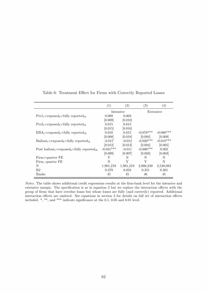
Table 6: Treatment Effect for Firms with Correctly Reported Losses

(1) (2) (3) (4)

Intensive ExtensivePre1t×exposedb×fully reportedib 0.009 0.003

[0.009] [0.010]Pre2t×exposedb×fully reportedib 0.015 0.015

[0.015] [0.016]EBAt×exposedb×fully reportedib 0.010 0.015 -0.078*** -0.086***

[0.008] [0.018] [0.004] [0.009]Bailoutt×exposedb×fully reportedib -0.017 -0.012 -0.020*** -0.018***

[0.012] [0.013] [0.004] [0.005]Post bailoutt×exposedb×fully reportedib -0.031*** -0.011 -0.006*** 0.002

[0.009] [0.007] [0.003] [0.003]Firm×quarter FE Y N N NFirm, quarter FE N Y Y NN 1,981,219 1,981,219 2,980,249 2,538,082R2 0.379 0.058 0.351 0.301Banks 45 45 46 45

Notes. The table shows additional credit regressions results at the firm-bank level for the intensive andextensive margin. The specification is as in equation 2 but we replace the interaction effects with thegroup of firms that have overdue loans but whose losses are fully (and correctly) reported. Additionalinteraction effects are omitted. See equations in section 3 for details on full set of interaction effectsincluded. *, **, and *** indicate significance at the 0.1, 0.05 and 0.01 level.

62

Table 7: Regression Results Firm-Bank Level: Intensive Margin

Growth rate of credit (1) (2) (3) (4) (5) (6)

Total credit Performing Non-perf New loanPre1t×exposedb -0.011 -0.010 -0.011 -0.000 -0.024

[0.008] [0.010] [0.008] [0.002] [0.015]Pre2t×exposedb -0.003 -0.005 -0.003 -0.000 -0.022

[0.010] [0.010] [0.010] [0.002] [0.014]EBAt×exposedb -0.020∗∗ -0.022∗ -0.022∗∗ 0.001 -0.039∗∗∗

[0.010] [0.013] [0.009] [0.002] [0.014]Bailoutt×exposedb -0.006 -0.008 -0.004 -0.002 -0.013

[0.006] [0.008] [0.007] [0.003] [0.011]Post bailoutt×exposedb 0.008 0.006 0.009 -0.002 0.004

[0.008] [0.012] [0.009] [0.002] [0.011]Pre1t×exposedb×underreportedib 0.008 0.001 0.018 0.007 -0.006 0.009

[0.013] [0.013] [0.012] [0.013] [0.007] [0.008]Pre2t×exposedb×underreportedib 0.008 0.006 0.021 0.010 -0.004 0.016

[0.023] [0.023] [0.025] [0.020] [0.007] [0.023]EBAt×exposedb×underreportedib 0.041∗∗∗ 0.044∗∗∗ 0.050∗∗∗ 0.038∗∗ 0.005 0.069∗∗∗

[0.013] [0.012] [0.019] [0.015] [0.009] [0.022]Bailoutt×exposedb×underreportedib 0.019 0.027∗ 0.027 0.035∗∗ -0.008 0.042∗∗

[0.019] [0.016] [0.019] [0.015] [0.011] [0.017]Post bailoutt×exposedb×underreportedib 0.005 0.016 0.023∗ 0.022 -0.007 0.030∗∗

[0.014] [0.011] [0.013] [0.014] [0.010] [0.012]Bank*quarter FE Y N N N N NFirm*quarter FE Y Y N Y Y YFirm, quarter FE N N Y N N NN 1,981,219 1,981,219 1,981,219 1,981,219 1,981,219 1,981,219R2 0.381 0.379 0.057 0.383 0.405 0.413Banks 45 45 45 45 45 45

Notes. The table shows credit regressions results at the firm-bank level. The dependent variable is thequarterly growth rate in total credit for a given firm-bank pair in columns (1)-(5). Columns (4) and (5)decompose total credit growth into performing and non-performing credit. These growth rates are definedas the quarterly change are scaled by lagged total credit: ∆cperfit /calli,t−1. Column 6 presents results froma linear probability model where the dependent variable is a dummy that is 1 if the number of loans in afirm-bank pair increases (conditional on an increase in loan volume). The explanatory variable exposedis a dummy that is 1 for banks exposed to the EBA shock. The sample period is 2009q1-2014q4. Pre 1and 2, EBA, bailout and post-bailout are dummies that identify the following time periods: The EBAshock (2011q4-2012q2), the bailout period (2012q-2012q4), two pre-periods and one post-bailout periodall of equal length. Underreported is a firm-bank dummy that identifies relationships subject to lossunderreporting in the four quarters prior to the EBA shock. All regressions include bank fixed effectsand firm-bank controls (see text for details). Standard errors in parentheses and are two-way clusteredby bank and firm. Additional interaction effects are omitted. See equations in section 3 for details onfull set of interaction effects included. *, **, and *** indicate significance at the 0.1, 0.05 and 0.01 level.

63

Table 8: Regression Results Firm-Bank Level: Robustness Checks

Growth rate of total credit (1) (2) (3) (4) (5)

OLS WLSPre1t×exposedb -0.009 -0.011 -0.009 -0.016* -0.026**

[0.008] [0.010] [0.011] [0.009] [0.011]Pre2t×exposedb -0.004 -0.003 -0.002 -0.018 -0.023**

[0.010] [0.013] [0.010] [0.011] [0.011]EBAt×exposedb -0.022** -0.020* -0.020 -0.029*** -0.038***

[0.010] [0.012] [0.013] [0.011] [0.010]Bailoutt×exposedb -0.009 -0.006 -0.005 -0.015* -0.012*

[0.006] [0.008] [0.008] [0.008] [0.007]Post bailoutt×exposedb 0.006 0.008 0.008 0.002 0.006

[0.007] [0.010] [0.012] [0.009] [0.008]Pre1t×exposedb×underreportedib 0.002 0.001 0.012 0.013 -0.003

[0.013] [0.014] [0.010] [0.008] [0.012]Pre2t×exposedb×underreportedib 0.006 0.006 0.024 0.012 0.005

[0.023] [0.028] [0.023] [0.016] [0.019]EBAt×exposedb×underreportedib 0.043*** 0.044*** 0.051*** 0.051*** 0.073***

[0.013] [0.014] [0.017] [0.015] [0.014]Bailoutt×exposedb×underreportedib 0.027 0.027 0.026 0.034*** 0.040***

[0.017] [0.019] [0.021] [0.010] [0.013]Post bailoutt×exposedb×underreportedib 0.016 0.016 0.021 0.014 0.029***

[0.012] [0.013] [0.014] [0.010] [0.009]Firm×quarter FE Y Y N N YFirm, quarter FE N N Y Y NRelationship controls N Y Y Y YFirm-level controls N N Y N NN 1,981,219 1,981,219 1,859,321 5,244,714 1,981,219R2 0.378 0.379 0.057 0.069 0.417Banks 45 45 45 45 45

Notes. The table shows additional credit regressions results at the firm-bank level for the intensivemargin. The dependent variable is the quarterly growth rate in total credit for a given firm-bankpair. The explanatory variable exposed is a dummy that is 1 for banks exposed to the EBA shock.Sample period is 2009q1-2014q4. Pre 1 and 2, EBA, bailout and post-bailout are dummies that identifythe following time periods: The EBA shock (2011q4-2012q2), the bailout period (2012q-2012q4), twopre-periods and one post-bailout period all of equal length. underreported is a dummy that identifiesrelationships subject to underreported losses in the four quarters prior to the EBA shock. All regressionsinclude bank fixed effects. Standard errors in parentheses and are two-way clustered by bank and firmwith the exception of column (2) which is clustered by bank-level. Column (4) does not restrict thesample to firms with multiple lending relationships. Column (5) weights by the square root of the loanbalance. Square root weighting is attractive because it does not give as much weight to the tail of verylarge firms as level weighting. Additional interaction effects are omitted. See equations in section 3 fordetails on the full set of interaction effects included. *, **, and *** indicate significance at the 0.1, 0.05and 0.01 level.

64

Table 9: Regression Results Firm-bank Level:Extensive Margin

Pr(relationship cut) (1) (2) (3)

EBAt×exposedb 0.057*** 0.056*** 0.058***[0.011] [0.011] [0.012]

Bailoutt×exposedb 0.041*** 0.042*** 0.043***[0.009] [0.008] [0.008]

Post bailoutt×exposedb 0.029*** 0.030*** 0.029***[0.010] [0.009] [0.009]

EBAt×exposedb×underreportedib -0.217*** -0.202*** -0.219***[0.034] [0.027] [0.057]

Bailoutt×exposedb×underreportedib -0.106*** -0.090*** -0.105**[0.033] [0.030] [0.047]

Post bailoutt×exposedb×underreportedib -0.053*** -0.041*** -0.050**[0.018] [0.015] [0.024]

Firm FE Y N YFirm controls N Y NN 2,973,566 2,538,082 2,973,566R2 0.706 0.137 0.706Banks 46 45 46

Notes. The table shows credit regressions results at the firm-bank level for the extensive margin (linearprobability model). The dependent variable is a dummy that turns one in the quarter when there is azero loan balance of performing credit. The explanatory variable exposed is a dummy that is 1 for banksexposed to the EBA shock. Pre period 1 and 2, EBA, bailout and post-bailout are dummies that identifythe following time periods: The EBA shock (2011q4-2012q2), the bailout period (2012q-2012q4), andone post-bailout period all of equal length. We cannot estimate pre-trends in this regression since wecondition on a sample of relationships that have positive loan balances in the pre-periods. underreportedis a dummy that identifies relationships subject to underreported losses in the four quarters prior tothe EBA shock. All regressions include bank and quarter fixed effects. Column 1 and 3 contain firmfixed effects. Column includes industry×quarter fixed effects and firm-level sales growth and leverageinteracted with the time period to allow for flexible time trends. Standard errors in parentheses andare two-way clustered by bank and firm. Additional interaction effects are omitted. See equation 2 insection 3 for details on full set of interaction effects included. *, **, and *** indicate significance at the0.1, 0.05 and 0.01 level.

65

Table 10: Pass-Through Into Employment and Investment: Persistence and Placebo Tests

(1) (2) (3) (4) (5)

Symmetric growth rate Employees2013 2014 2011 2009 2008

∆ log crediti -0.555** 3.326 -0.028 -0.653 0.102[0.218] [6.853] [0.045] [0.978] [0.074]

Controls Y Y Y Y YIndustry, size FE Y Y Y Y YFirst stage F-statistic 8.8 0.277 116.7 1.5 6N 105,170 93,729 126,595 126,595 124,478

Notes. The table shows regression results at the annual firm-level for different years. The dependentvariable is the Davis-Haltiwanger (1992) symmetric growth rate of employment. We instrument for thelog change in credit using the (normalized) firm-level borrowing share from banks exposed to the EBAshock prior to the shock. Relative to table 3 we only vary the year of the dependent and independentvariables. Controls consist of firm-size and 2-digit industry FE, as well as firm-level log total assets,interest/ebitda, capital/assets, currrent ratio, cash/assets and sales growth all averaged over 2008-2010.Lag refers to the lag of the dependent variable. Standard errors are clustered by firm-size bucket.Standard errors in parentheses. *, **, and *** indicate significance at the 0.1, 0.05 and 0.01 level.

66

Table 11: Descriptive Statistics: New Lending Operations

Non-subsidized firms Subsidized firms Matches p-valueInterest rate 7.68 5.70 5.57

(3.55) (2.37) (2.61)Amount (m) 0.09 0.05 0.05 0.99

(2.51) (0.19) (0.21)Maturity (days) 377.30 313.45 280.36 1

(876.80) (720.03) (596.54)Collateralized 0.43 0.37 0.28 1

(0.49) (0.48) (0.45)Days rate fixed 114.24 91.85 97.36 1

(245.87) (78.26) (122.91)Total (m) 0.38 0.28 0.14

(4.12) (1.97) (0.48)Rel length (months) 76.76 79.55 85.24

(36.31) (36.08) (34.01)Existing borrower 0.85 0.98 0.83

(0.36) (0.15) (0.37)Main lender 0.51 0.51 0.54

(0.50) (0.50) (0.50)Subsidy (b.p.) 302.67

(153.63)N 1,291,224 276,416 60,336

Notes. The table show descriptive statistics for new lending operations from June 2012 -May 2015. Thefirst column shows all operations that are neither subsidized nor used as a matched control. The secondcolumn shows lending operations that we identify as subsidized according to the matching proceduredescribed in text. The third column shows lending operations to investment-grade firms that serve asmatches. The last column shows p-values on one sided t-tests between subsidized and matched controls inthe direction that we would expect to lower interest rates (lower amount, lower maturity, not collteralized,fewer days fixed rate). Total refers to the total amount of new loans in a given firm-bank-month triple,while amount refers to the size of an individual loan. Subsidy (measured in basis points) is the averagedifference in interest rates on subsidized loans and loans to firms in the worst rating category accordingto a credit rating model for non-financial firms by Antunes et al. (2016).

67

Table 12: Pass-Through Into Employment and Investment

Panel a (1) (2) (3) (4) (5)

Labor Capital Materials Services Tech. efficiency∆ log credit 0.097** 0.692*** 0.138** 0.284** -0.081

[0.018] [0.105] [0.024] [0.053] [0.055]Lag -0.062** 0.046*** -0.317*** 0.028** -0.326***

[0.012] [0.005] [0.005] [0.008] [0.023]Controls Y Y Y Y YIndustry, size FE Y Y Y Y YN 78,288 78,288 78,288 78,288 78,288First-stage F statistic 195.8 195.8 195.8 195.8 195.8

Panel b (1) (2) (3) (4)

Labor gap Capital gap Materials gap Services gap∆ log credit -0.100** -0.195** -0.020 0.012

[0.020] [0.033] [0.062] [0.033]Controls Y Y Y YIndustry, size FE Y Y Y YN 102,495 102,495 102,495 102,495First-stage F statistic 193 193 193 193

Notes. The table shows IV regression results at the annual firm-level in 2012. All the dependent variablesare changes in logs. All variables are deflated according to procedure described in online appendix. Inpanel b, dependent variables are firm-level gaps between output elasticities and revenue shares. We usethe log change of the absolute value of the gap (to allow for negative gaps). We instrument for thelog change in credit using the (normalized) firm-level borrowing share from banks exposed to the EBAshock prior to the shock. Controls consist of firm-size and 2-digit industry FE, as well as firm-level logtotal assets, interest/ebitda, capital/assets, currrent ratio, cash/assets and sales growth all averaged over2008-2010. Lag refers to the lag of the dependent variable. Technical efficiency is the production functionresidual. In panel b we control for firm-level sales cylicality and productivity volatility. Standard errorsare clustered by industry. Standard errors in parentheses. *, **, and *** indicate significance at the 0.1,0.05 and 0.01 level.

68

Table 13: Robustness: Spillovers

(1) (2) (3) (4) (5) (6)

2-digit 4-digit 1-digit-districtSales Capital Sales Capital Sales Capital

Industry share of -0.093*** -0.104*** -0.139*** -0.085*** -0.122*** -0.117**underreported firms [0.018] [0.019] [0.020] [0.023] [0.047] [0.046]

N 43,273 43,273 43,273 43,273 43,273 43,273First-stage 3381 3381 2531 2531 549.8 549.8

Notes. The table shows IV regression results at the firm-level for 2012. Share underreported refers tothe asset-weighted share of distressed, underreported firms. We vary the definition of industry. The lastcolumn shows results for creating district-1-digit industry categories. We instrument for this variableusing the average firm-level borrowing share from EBA banks. We standardize the share such that thecoefficients should be interpreted as the effect of increasing the industry-share of underreported firms bya standard deviation. The dependent variables are all in log changes and deflated. Controls consist offirm-size bucket FE as well as firm-level log total assets, interest/ebitda, capital/assets, currrent ratio,cash/assets and sales growth all averaged over 2008-2010. Robust standard errors in parentheses. *, **,and *** indicate significance at the 0.1, 0.05 and 0.01 level.

69

Figure 4: Decomposition of Underreported Losses by Mechanism

0.2

.4.6

Frac

tion

2009m7 2011m1 2012m7 2014m1 2015m7

Excess length SwapsExcess length - same amount

Notes. The graph shows the decomposition of underreported losses by the mechanisms discussed insection 2. Excess length refers to spells of overdue reporting in a bucket that exceed the permissiblelength (e.g. loan reported to be overdue 3-5 months for 4 months in a row.). Excess length - same amountrefers to spells that exceed the permissible length where the loan balance does not change. Swaps refer tocases where there is a decrease in the overdue balance equal to an increase in the performing loan balance.This captures the last mechanism where banks grant new credit in exchange for the firm repaying thelongest overdue credit portion. All numbers are scaled by the total amount of excess mass.

Figure 5: Histogram of Firm-Level Exposure to EBA Shock

02

46

8D

ensi

ty

0 .5 1 1.5 2 2.5Exposure

Notes. The graph shows a histogram of the continuous exposure measure for firms with underreportedlosses. The exposure measure is the share of credit coming from banks exposed to the EBA shock in 2010.We standardize the measure to have unit variance. The peaks at 0 and 2.25 represent firms borrowingexclusively from exposed and non-exposed banks.

70

Figure 6: Additional Results on Underreporting of Loan Losses

010

2030

40Re

port

ed ti

me

over

due

(mon

ths)

0 10 20 30 40Time overdue (months)

(a) Evidence of Reporting Management fromSingle-Loan Relationships

1020

3040

50Le

ngth

of s

pell

(mon

ths)

2009m1 2011m1 2013m1 2015m1

Underreported losses Overdue

(b) Persistence of Unrecognized Losses

Notes. Panel a graph compares the average constructed time overdue (x-axis) with the reported timeoverdue (y-axis) for the sample of relationships with a single loan. In this sample we can track how longa loan has been overdue by simply counting the number of months the loan has been reported as overduein the data. Panel b shows the average length of spells of overdue (or non-performing) and unrecognizedlosses at the firm-bank level. A spell is measured as a period of time in which the firm-bank relationshipsfeature either some overdue loan balance, and an unrecognized loss respectively. We allow reporting gapsof up to three months.

71

Figure 7: Long-run Trends: Underreported vs Non-underreported Firms

-.10

.1.2

Prob

(exi

t)

0 2 4 6 8 10Year since first default

UnderreportedNot underreported

(a) Probability of exit

-.2-.1

0.1

Shar

e ov

erdu

e

0 2 4 6 8 10Year since first default

UnderreportedNot underreported

(b) Share of loans overdue

-.01

-.005

0.0

05Re

turn

on

asse

ts

0 2 4 6 8 10Year since first default

UnderreportedNot underreported

(c) Return on assets

-.05

0.0

5.1

.15

Sale

s gr

owth

0 2 4 6 8 10Year since first default

UnderreportedNot underreported

(d) Sales growth

Notes. The graphs show the average evolution of firm-level measures over time. We plot the 95 confidenceintervals of the residualized mean for each group. The variables are residualized on year×industry andfirm size. The x-axis are years following the first time we observe an overdue loan in the data (for agiven firm). The upwards trend in sales is likely due to a survivorship bias since firms that exit drop outof the sample.

72

Figure 8: Liquidity and Credit Pre-trends

-.4-.2

0.2

.4Co

effic

ient

2007 2008 2009 2010

(a) Current Ratio

-.005

0.0

05.0

1Co

effic

ient

2007 2008 2009 2010

(b) Cash/Assets

-.1-.0

50

.05

.1Q

uart

er*f

irm F

E

2009q1 2009q3 2010q1 2010q3 2011q3

Underreported

2011q1

Not UnderreportedNo NPL

(c) Firm×time fixed effects

Notes. Panels (a) and (b) show results from a dynamic differences-in-differences specification wherewe interact the firm-level borrowing share from banks exposed to the EBA shock with year dummiesfor the period prior to the EBA shock. We run the regression in the subset of firms subject to lossunderreporting. The two panels show two different liquidity measures. Standard errors are clustered atthe firm-level. Panel (c) shows the fixed effects from a regression that decomposes quarterly firm-bankcredit growth into a bank and firm×quarter component. The firm×time fixed effects can be interpretedas a measure of firm-level credit demand. No NPL refers to firms without overdue loans.

73

Figure 9: Additional Results: Firm-level Regression

-.06

-.03

0.0

3.0

6Tr

eatm

ent e

ffect

2010Q2-Q42011Q1-Q3

EBABailout

2013Q2-Q4

Performing Non-Performing

(a) Decomposition of Credit

Notes. The graphs show treatment effects at the quarterly firm-level. The dependent variable is thequarterly log of performing and non-performing credit. We plot the coefficients on the interactiontreatmenti×quartert×underreportedi, which are the treatment effects for the group of firms subject toloss underreporting. The vertical lines denote the EBA announcement and compliance deadline. Thespecification, equation 3, includes the full set of interactions, industry×quarter and firm fixed effects, aswell as firm-level controls interacted with quarter. All coefficients should be interpreted as changes inthe dependent variable relative to the (normalized) base quarter 2011Q3. Standard errors are clusteredat the firm-level. N= 1,346,771.

Figure 10: First-Time Loan Subsidies

.2.2

5.3

.35

.4.4

5

56

78

9Fr

actio

n (d

ebt)

, per

cent

(def

ault)

-3 -2 -1 0 1 2 3t(years)

Default risk in percent (left) Debt/EBITDA (left)Interest/EBITDA (right)

(a) Evolution of Firm-Characteristics AroundFirst Subsidy

0.2

.4.6

.81

Frac

tion

subs

idiz

ed

-3 -2 -1 0 1 2 3t(years)

(b) Persistence of Loan Subsidies

Notes. Panel a shows the average evolution of firm-level financial health indicators in the years aroundthe year a firm first receives a subsidized loan (t = 0). Panel b shows the fraction of subsidized newloans a firm receives following the year a firm first receives a subsidized loan (t = 0).

74

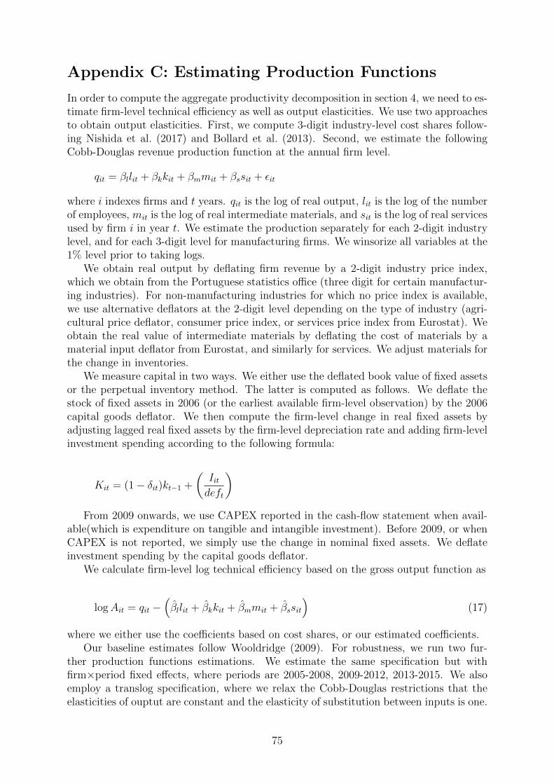
Appendix C: Estimating Production Functions

In order to compute the aggregate productivity decomposition in section 4, we need to es-timate firm-level technical efficiency as well as output elasticities. We use two approachesto obtain output elasticities. First, we compute 3-digit industry-level cost shares follow-ing Nishida et al. (2017) and Bollard et al. (2013). Second, we estimate the followingCobb-Douglas revenue production function at the annual firm level.

qit = βllit + βkkit + βmmit + βssit + εit

where i indexes firms and t years. qit is the log of real output, lit is the log of the numberof employees, mit is the log of real intermediate materials, and sit is the log of real servicesused by firm i in year t. We estimate the production separately for each 2-digit industrylevel, and for each 3-digit level for manufacturing firms. We winsorize all variables at the1% level prior to taking logs.

We obtain real output by deflating firm revenue by a 2-digit industry price index,which we obtain from the Portuguese statistics office (three digit for certain manufactur-ing industries). For non-manufacturing industries for which no price index is available,we use alternative deflators at the 2-digit level depending on the type of industry (agri-cultural price deflator, consumer price index, or services price index from Eurostat). Weobtain the real value of intermediate materials by deflating the cost of materials by amaterial input deflator from Eurostat, and similarly for services. We adjust materials forthe change in inventories.

We measure capital in two ways. We either use the deflated book value of fixed assetsor the perpetual inventory method. The latter is computed as follows. We deflate thestock of fixed assets in 2006 (or the earliest available firm-level observation) by the 2006capital goods deflator. We then compute the firm-level change in real fixed assets byadjusting lagged real fixed assets by the firm-level depreciation rate and adding firm-levelinvestment spending according to the following formula:

Kit = (1− δit)kt−1 +

(Iitdeft

)From 2009 onwards, we use CAPEX reported in the cash-flow statement when avail-

able(which is expenditure on tangible and intangible investment). Before 2009, or whenCAPEX is not reported, we simply use the change in nominal fixed assets. We deflateinvestment spending by the capital goods deflator.

We calculate firm-level log technical efficiency based on the gross output function as

logAit = qit −(βllit + βkkit + βmmit + βssit

)(17)

where we either use the coefficients based on cost shares, or our estimated coefficients.Our baseline estimates follow Wooldridge (2009). For robustness, we run two fur-

ther production functions estimations. We estimate the same specification but withfirm×period fixed effects, where periods are 2005-2008, 2009-2012, 2013-2015. We alsoemploy a translog specification, where we relax the Cobb-Douglas restrictions that theelasticities of ouptut are constant and the elasticity of substitution between inputs is one.

75

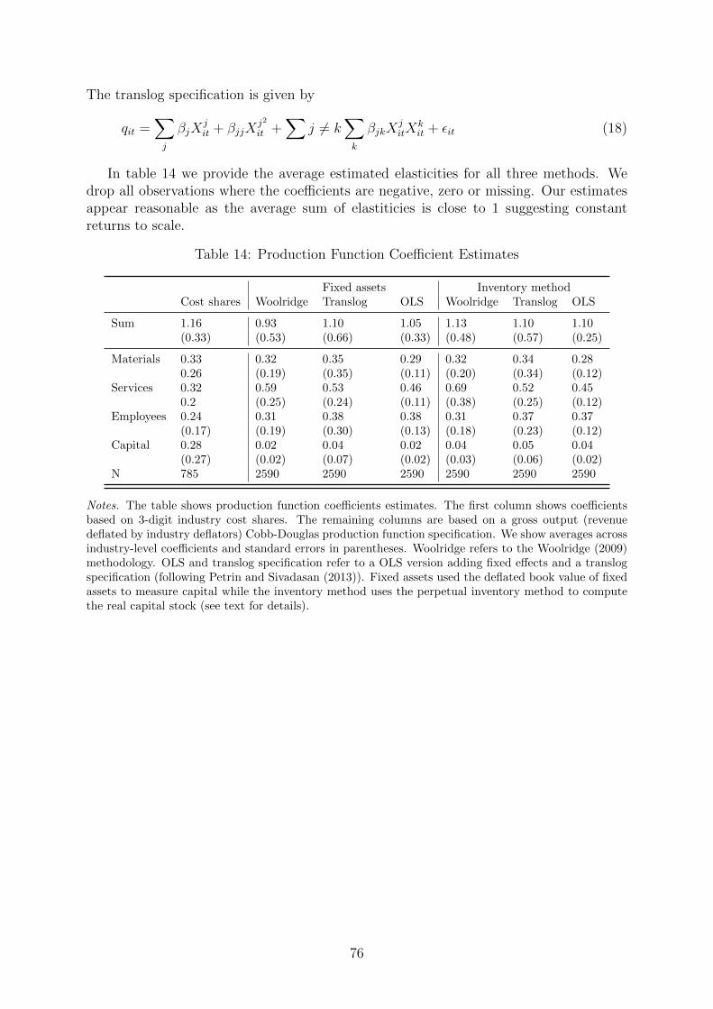
The translog specification is given by

qit =∑j

βjXjit + βjjX

j2

it +∑

j 6= k∑k

βjkXjitX

kit + εit (18)

In table 14 we provide the average estimated elasticities for all three methods. Wedrop all observations where the coefficients are negative, zero or missing. Our estimatesappear reasonable as the average sum of elastiticies is close to 1 suggesting constantreturns to scale.

Table 14: Production Function Coefficient Estimates

Fixed assets Inventory methodCost shares Woolridge Translog OLS Woolridge Translog OLS

Sum 1.16 0.93 1.10 1.05 1.13 1.10 1.10(0.33) (0.53) (0.66) (0.33) (0.48) (0.57) (0.25)

Materials 0.33 0.32 0.35 0.29 0.32 0.34 0.280.26 (0.19) (0.35) (0.11) (0.20) (0.34) (0.12)

Services 0.32 0.59 0.53 0.46 0.69 0.52 0.450.2 (0.25) (0.24) (0.11) (0.38) (0.25) (0.12)

Employees 0.24 0.31 0.38 0.38 0.31 0.37 0.37(0.17) (0.19) (0.30) (0.13) (0.18) (0.23) (0.12)

Capital 0.28 0.02 0.04 0.02 0.04 0.05 0.04(0.27) (0.02) (0.07) (0.02) (0.03) (0.06) (0.02)

N 785 2590 2590 2590 2590 2590 2590

Notes. The table shows production function coefficients estimates. The first column shows coefficientsbased on 3-digit industry cost shares. The remaining columns are based on a gross output (revenuedeflated by industry deflators) Cobb-Douglas production function specification. We show averages acrossindustry-level coefficients and standard errors in parentheses. Woolridge refers to the Woolridge (2009)methodology. OLS and translog specification refer to a OLS version adding fixed effects and a translogspecification (following Petrin and Sivadasan (2013)). Fixed assets used the deflated book value of fixedassets to measure capital while the inventory method uses the perpetual inventory method to computethe real capital stock (see text for details).

76