when opportunity knocks - cross-sectional return ...cfr.ivo-welch.info/readers/2017/reibnitz.pdf ·...
TRANSCRIPT
When Opportunity Knocks:
Cross-Sectional Return Dispersion and Active Fund Performance
Anna von Reibnitz*
Australian National University
14 September 2015
Abstract Active opportunity in the market, measured by cross-sectional dispersion in stock returns, significantly influences fund performance. Active strategies have the greatest impact on returns during periods of high dispersion, when alpha produced by the most active funds significantly exceeds that produced in other months. The outperformance of the most relative to the least active funds is also concentrated in months of high dispersion. Deciding when to invest in active funds, therefore, can be as important to generating outperformance as deciding which funds to invest in. Switching between highly active and passive funds based on dispersion produces significant alpha of over 2.7% p.a. after fees. This paper adds a new dimension to understanding how active funds can be used to generate value, by combining identification of which managers have the greatest potential to outperform the market with insight into when the market is most conducive to outperformance.
JEL Classification: G11, G14, G20, G23
Keywords: Mutual funds; return dispersion; active management * Corresponding author: Anna von Reibnitz, Research School of Finance, Actuarial Studies and Statistics, Australian National University, Canberra, ACT 0200, phone: +61 2 6125 4626, fax: +61 2 6125 0087, email: [email protected]. I thank Jenni Bettman, Honghui Chen (discussant), Jozef Drienko, Stephen Sault, Tom Smith, Ivo Welch, three anonymous referees and seminar and conference participants at the 2014 FMA Annual Meeting, the 2013 Australasian Finance and Banking Conference, and the Australian National University for helpful comments and suggestions. I also thank Ken French, Antti Petajisto, Robert Stambaugh and Russ Wermers for providing data on factor returns, Active Share and characteristic-based benchmarks through their websites.
1
The business case of the funds management industry is dependent on adding value. Passive
fund managers charge modest fees for exposing investors to the returns of a diversified
market index. Active managers charge higher fees with the promise of something more.
Where a passive manager will simply track a market index, an active manager will pursue
active bets that attempt to focus investments on better performing stocks, while avoiding the
worst performers.
Underlying this is a presumption that active managers are able to design and carry out
active strategies that successfully outperform passive alternatives. Evidence to support this on
a broad scale has proved elusive, with the majority of studies concluding that, on average,
actively managed funds actually produce inferior risk-adjusted performance after expenses.1
Nonetheless, the active funds industry continues to thrive. Significant efforts have been
devoted to identifying those active managers able to generate returns that justify their fees.2
In this context, an emerging body of literature suggests that, while active funds as a whole
underperform their benchmarks after fees, managers who pursue the most active strategies
achieve superior risk-adjusted performance.3
Thus far, however, little attention has been paid to the impact that the market environment
has on the effectiveness of active strategies. This paper adds a new dimension to
understanding how active funds can be used to generate value, by combining identification of
which managers have the greatest potential to outperform the market with insight into when
the market environment is most conducive to outperformance. In doing so, we show that an
investor’s choice of when to invest in active funds can be as important to generating
outperformance as the choice of which funds to invest in.
1 See, e.g., Malkiel (1995), Gruber (1996) and Carhart (1997). 2 See, e.g., Pástor and Stambaugh (2002), Kacperczyk and Seru (2007), Kacperczyk, Sialm, and Zheng (2008), Baker et al. (2010), Huang, Sialm, and Zhang (2011), Chen, Desai, and Krishnamurthy (2013), Gupta-Mukherjee (2013), Del Geurcio and Reuter (2014), Kacperczyk, van Nieuwerburgh, and Veldkamp (2014b) and Koijen (2014). 3 See, e.g., Wermers (2003a), Kacperczyk, Sialm, and Zheng (2005), Brands, Brown, and Gallagher (2005), Cremers and Petajisto (2009), Huij and Derwall (2011), Amihud and Goyenko (2013) and Cremers et al. (2015).
2
If the superior performance by managers who pursue highly active bets is an indication of
skill, one would expect that the additional performance produced by these managers would be
greatest during times in which the impact of active bets is strongest, specifically in times of
high cross-sectional dispersion in stock returns. The presence of dispersion is central to
generating outperformance: active bets cannot produce performance that differs discernibly
from the market unless the returns of stocks are sufficiently dispersed.4 When stock returns
are similar, tilting towards higher performers is of little advantage, and outperforming the
market even before fees is therefore unlikely.5 As dispersion increases, however, so does the
potential for a skilled manager to outperform, due to the payoff from increasing weights in
those stocks that will go on to outperform the market as a whole.
There are further reasons to suggest that high dispersion may provide an environment
where managers with superior insight and analytical ability can gain particular advantage. A
number of studies find a positive relation between return dispersion and future volatility at
both the market (e.g., Bekaert and Harvey, 1997 for developed markets; Stivers, 2003) and
firm (e.g., Connolly and Stivers, 2006) levels. Bessembinder, Chan, and Seguin (1996) find a
positive relation between dispersion, used to gauge the arrival of firm-specific information,
and trading volume for individual stocks, as investors seek to capitalize on such information.
Loungani, Rush, and Tave (1990) and Brainard and Cutler (1993) show that high dispersion
is a significant predictor of unemployment caused by sectoral shifts, during which resource
reallocation shocks trigger a range of company revaluations. Such findings point to periods of
high dispersion as a natural setting to detect skill: a market in which the ability to capture,
interpret and act on information signals can strongly differentiate a manager from their peers.
4 In referring to active bets, we focus on strategies that aim to capitalize on the superior information and skill of the manager in identifying high performing stocks. This relates to the informed or “impatient trading” component of security selection identified by Da, Gao, and Jagannathan (2011), as opposed to the “liquidity provision” component, for which opportunity is less likely to be reflected in return dispersion metrics. 5 At the extreme, zero dispersion in returns is akin to having only one stock in which to invest. As that stock also constitutes the market, even a manager with perfect foresight could not invest in equities that outperform (or underperform) the benchmark, making active strategies futile.
3
To examine the importance of the market environment, we condition tests of the relation
between fund activeness and performance on the level of cross-sectional dispersion in stock
returns. We characterize dispersion environments by sorting the months of our sample into
quintiles based on their level of return dispersion at the start of the month. We then examine
performance in the subsequent month, sorting funds into quintile portfolios of differing
activeness using the (1-R2) measure of Amihud and Goyenko (2013), where R2 is obtained by
regressing fund returns on performance models. Over our 42 year sample (1972 to 2013) of
active U.S. equity mutual funds, we show that the positive relation between fund activeness
and performance is strongly dependent on the level of return dispersion in the market. In
times of low dispersion, in which active strategies produce little payoff, the difference in
performance between the most and least active funds is not significant. In months of high
dispersion, in which active bets have the greatest impact on returns, a portfolio of the funds
with the most active strategies significantly outperforms a portfolio with the least active
strategies. In other words, the superior risk-adjusted performance of the most active funds is
concentrated in times of high active opportunity.
In addition, we find a positive relation between return dispersion and subsequent fund
performance that increases with the activeness of a fund’s strategies. The most active fund
portfolio achieves significantly greater alpha during months belonging to the highest
dispersion quintile than it does during other months. The use of multivariate panel regressions
confirms that, after controlling for fund-level characteristics, the positive relation between
fund activeness and performance is considerably more pronounced during the months in the
highest dispersion quintile than in the remaining months of the sample.
Our results are robust to alternative measures of performance, dispersion and activeness,
and hold across sub-periods. Specifically, our findings are qualitatively consistent when
performance is estimated using raw returns, Fama-French (1993) and Carhart (1997) (FFC)
4
four-factor alpha, Cremers, Petajisto, and Zitzewitz (2013) (CPZ) four-factor alpha, or the
Characteristic Selectivity (CS) measure of Daniel et al. (1997); when dispersion is measured
using equal or value weights from either S&P 500 index constituents or a broader universe of
NYSE, Amex or Nasdaq listed stocks; when activeness is derived from selectivity or the
Active Share measure of Cremers and Petajisto (2009); when using alternative sample
periods; and after controlling for business cycle fluctuations.
A long-term switching strategy that combines knowledge of fund R2 and return dispersion
produces significantly positive risk-adjusted returns. Investing in the most active portfolio of
funds when dispersion in the prior month is ranked in the top 20% of months over the previous
ten years, and otherwise investing passively in funds that track the S&P 500 index, produces
significant FFC and CPZ alphas of over 1.8% p.a. after all fees. When active investment is
isolated to the funds in the most active portfolio with the best past performance, alpha from
the switching strategy increases to over 2.7% p.a. after fees, irrespective of the performance
model. In all cases, alpha produced from this highly active/passive switching strategy is
considerably greater than the alpha achieved by investing in highly active funds throughout.
The ability of high dispersion in one month to predict performance in the next is enabled
by significant persistence in high dispersion environments. As a result, there is little risk that
a positive response to high dispersion in one month would be undermined by a large drop in
dispersion in the subsequent month. This is important as, consequently, our strategy does not
require the ability to predict high dispersion before it first occurs, which is of significant
value to fund managers and fund investors alike.
We argue that knowledge of active opportunity is useful both ex ante and ex post, as it
provides valuable information about the capacity in the market to generate alpha. Ex ante, in
addition to being used by managers in the formation of active bets, it can be used by investors
in conjunction with measures of fund activeness to provide a more informed signal for
5
whether and when to invest in active funds. Specifically, where measures of activeness can
highlight funds with a greater potential to outperform passive benchmarks, measures of
dispersion can highlight when that outperformance is most likely to be realized.
Information on return dispersion can also be of significant value ex post. Managerial skill
might not be a sufficient condition for outperforming the benchmark, as the success of an active
strategy will depend on market conditions. If a sample period is dominated by low dispersion
and, consequently, low active opportunity, a skilled manager could appear to possess no skill
based on performance alone. Knowledge of the dispersion environment is therefore of use to
researchers, investors and practitioners ex post in the evaluation of fund performance.
In providing the first examination of whether funds that are the most active produce
superior risk-adjusted performance when active opportunity, and active risk, is greatest, our
paper combines and extends two separate strands of research. The first examines the positive
relation between fund activeness and performance. The second examines the role of cross-
sectional stock return dispersion in creating opportunity for active managers.
The literature shows a positive relation between the degree of activeness and performance,
where activeness is derived from return based measures such as tracking error (e.g., Wermers,
2003a) or fund portfolio holdings (e.g., Kacperczyk, Sialm, and Zheng, 2005; Brands, Brown,
and Gallagher, 2005). Cremers and Petajisto (2009) introduce a metric called “Active Share,”
defined as the proportion of a fund’s holdings that diverges from its benchmark, and find it to
be positively related to performance. Recent studies have turned to R2 to gauge activeness.6
More active funds pursue strategies that cause greater deviation from the benchmark factors of
the performance model, resulting in lower values of R2. Amihud and Goyenko (2013) find a
positive relation between mutual fund “selectivity,” as measured by (1-R2), and fund alpha.
The role of return dispersion in generating alpha has gained attention among practitioners
in recent years. In 2010, Russell Investments and Parametric Portfolio Associates launched
6 See, e.g., Titman and Tiu (2011) and Sun, Wang, and Zheng (2012) in the context of hedge funds.
6
the Russell-Parametric Cross-Sectional Volatility Indexes (“CrossVol”) to help investors
assess the alpha opportunity and active risk present in the market. The majority of studies
relating dispersion to fund performance, however, focus on the positive relation between
dispersion in stock returns and the dispersion in the performance of active funds (e.g., de
Silva, Sapra, and Thorley, 2001; Ankrim and Ding, 2002; Bouchey, Fjelstad, and Vadlamudi,
2011). Gorman, Sapra, and Weigand (2010) show that stock return dispersion is positively
related to the subsequent dispersion of stock alphas. But little consideration has been given to
the proportion, or attributes, of managers who successfully add value in times of high cross-
sectional dispersion in stock returns.
One related study that touches on these two strands of literature is Petajisto (2013), who
finds that dispersion positively predicts the subsequent average returns of funds classified
using Active Share as “active stock pickers.” Our paper differs from the aspect touched on by
Petajisto (2013) in three important respects. First, Petajisto (2013) looks at fund returns in
excess of their benchmarks that are not adjusted for risk. We examine the relation between
dispersion and subsequent risk-adjusted performance, using alpha from the four-factor FFC
and CPZ models. Analysis of four-factor alphas provides a more comprehensive test of
outperformance, as the size, value and momentum factors contained in these models
themselves represent cross-sectional differences in asset returns. Measuring performance using
these alphas therefore allows us to show that the most active managers can capitalize on
additional sources of high dispersion beyond those between small and big stocks, value and
growth stocks, and stocks with high and low past returns. Second, we avoid the assumption
that the overall relation between dispersion and subsequent fund performance is approximately
linear, by separating our sample period into quintiles of differing dispersion and examining
performance within each quintile. In doing so, we show that only the highest dispersion
quintile has considerable stability from one month to the next, suggesting that the use of

7
dispersion as an indicator of its magnitude in the coming month should be restricted to the
months in which dispersion is at its highest. Finally, we provide evidence that an ex ante
strategy of switching between highly active and passive no-load funds based on the dispersion
environment produces significantly positive alpha, which remains at over 2.7% p.a. after
accounting for all active and passive fees.
1. Measuring dispersion, fund activeness and performance
1.1. Calculating cross-sectional return dispersion
To measure the opportunity set available to active funds, we calculate the cross-sectional
dispersion in stock returns over a calendar month. Return dispersion in month t (RDt) is
calculated using an equally weighted cross-sectional standard deviation measure:
( )∑=
−−
=n
imtitt RR
nRD
1
2
1
1 (1)
where n is the number of S&P 500 constituents in month t, Rit is the return to an individual
S&P 500 constituent i in month t, and Rmt is the equally weighted average return on S&P 500
constituents in month t.7 In what follows, we test whether the return dispersion in one month
predicts performance in the next. Months are therefore ranked according to their level of
cross-sectional return dispersion at the end of the previous month (RDt-1).8 Based on this
ranking, five dispersion quintiles Q1 (low RDt-1) through to Q5 (high RDt-1) are created.
1.2. Measuring fund activeness
To determine the activeness of a fund’s strategies, we employ the method of Amihud and
Goyenko (2013) and use a fund’s R2 from regressing its returns on multifactor benchmark
7 The S&P 500 is chosen as, consistent with Sensoy (2009) among others, it is the most common fund benchmark in our sample. As discussed in Section 4, results are similar using a value-weighted dispersion measure, as well as when dispersion is calculated from a broader universe of all stocks listed on the NYSE, Amex or Nasdaq. 8 As discussed in Section 2.2, there is significant persistence in the high dispersion quintile between months t-1 and t. Employing a one month lag therefore allows for a manager to identify the move to a high dispersion environment and react by implementing an active strategy in the subsequent month.
8
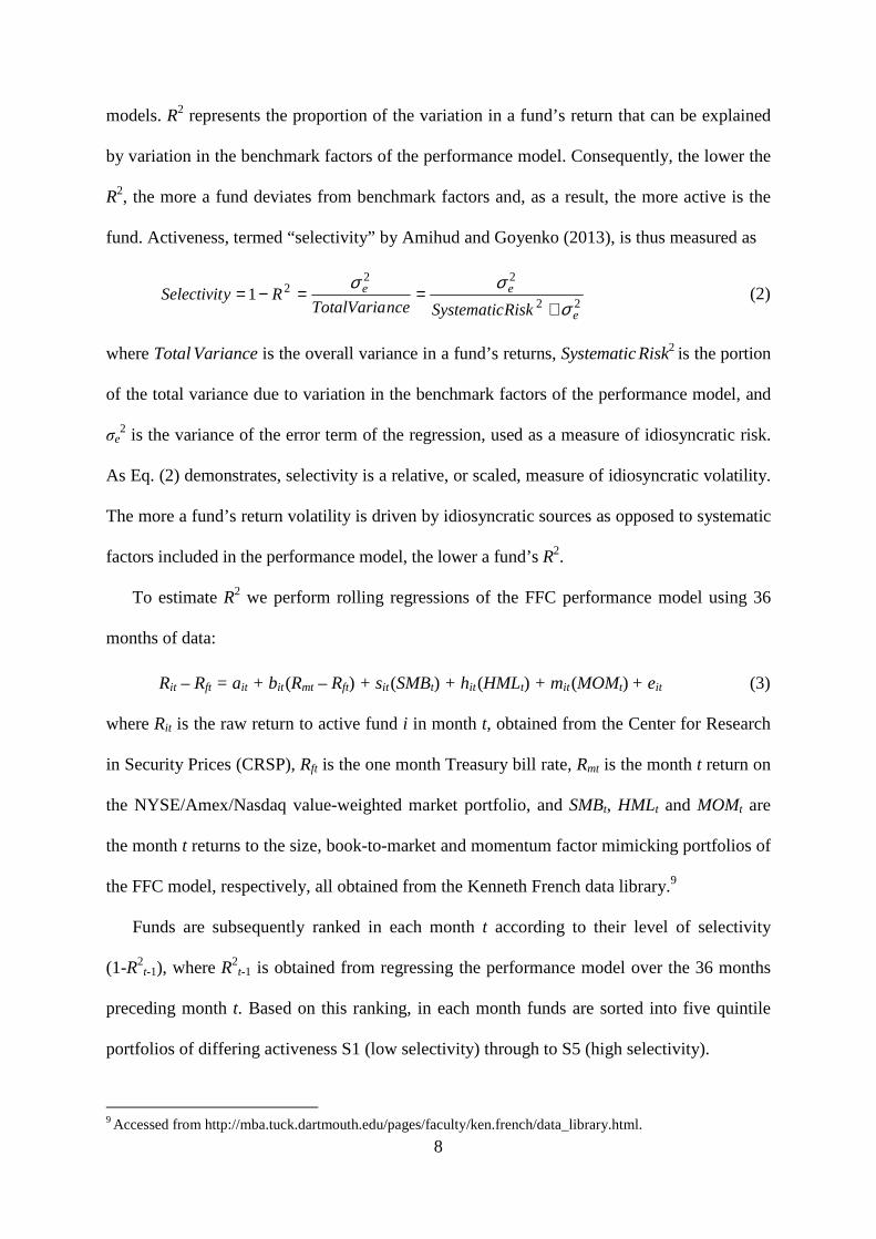
models. R2 represents the proportion of the variation in a fund’s return that can be explained
by variation in the benchmark factors of the performance model. Consequently, the lower the
R2, the more a fund deviates from benchmark factors and, as a result, the more active is the
fund. Activeness, termed “selectivity” by Amihud and Goyenko (2013), is thus measured as
22
2221
e
ee
RiskSystematicnceTotalVariaRySelectivit
σσσ
+==−= (2)
where Total Variance is the overall variance in a fund’s returns, Systematic Risk2 is the portion
of the total variance due to variation in the benchmark factors of the performance model, and
σe2 is the variance of the error term of the regression, used as a measure of idiosyncratic risk.
As Eq. (2) demonstrates, selectivity is a relative, or scaled, measure of idiosyncratic volatility.
The more a fund’s return volatility is driven by idiosyncratic sources as opposed to systematic
factors included in the performance model, the lower a fund’s R2.
To estimate R2 we perform rolling regressions of the FFC performance model using 36
months of data:
Rit – Rft = ait + bit (Rmt – Rft) + sit (SMBt) + hit (HMLt) + mit (MOMt) + eit (3)
where Rit is the raw return to active fund i in month t, obtained from the Center for Research
in Security Prices (CRSP), Rft is the one month Treasury bill rate, Rmt is the month t return on
the NYSE/Amex/Nasdaq value-weighted market portfolio, and SMBt, HMLt and MOMt are
the month t returns to the size, book-to-market and momentum factor mimicking portfolios of
the FFC model, respectively, all obtained from the Kenneth French data library.9
Funds are subsequently ranked in each month t according to their level of selectivity
(1-R2t-1), where R2
t-1 is obtained from regressing the performance model over the 36 months
preceding month t. Based on this ranking, in each month funds are sorted into five quintile
portfolios of differing activeness S1 (low selectivity) through to S5 (high selectivity).
9 Accessed from http://mba.tuck.dartmouth.edu/pages/faculty/ken.french/data_library.html.

9
1.3. Performance measurement
Having sorted the months of our sample into quintiles based on cross-sectional return
dispersion (RDt-1), and sorted funds each month into quintile portfolios based on their level of
selectivity (1-R2t-1), we then examine whether the performance of funds of differing levels of
activeness is sensitive to the dispersion environment. These tests are described in Section 3.
2. Data and sample selection
2.1. Mutual fund data and sample selection
Our sample period covers the 42 years from January 1972 to December 2013.10 As we use
the prior 36 months of returns in the computation of R2, data are collected from 1969.
Monthly fund return data are from the CRSP Survivor-Bias-Free Mutual Fund Database.
These are net returns after subtracting all management expenses and 12b-fees. CRSP
provides return data at the individual share class level rather than the overall fund portfolio
level. Consequently, when a fund has multiple share classes, we weight the monthly return of
each class by its beginning of the month total net asset value to compute overall fund return.11
We restrict our sample to actively managed domestic U.S. equity mutual funds using a
combination of investment style classifications. CRSP provides three different classifications
over our sample period: Wiesenberger objective codes until 1993, Strategic Insight Objective
Codes from 1993 to 1998, and Lipper Objective Codes from 1998 onwards. In addition,
Lipper Asset and Classification Codes are available from 1999. These classifications are used
to eliminate balanced, bond, index, international and sector funds.12 As we are concerned
10 1972 is chosen as the start of our sample as, prior to this, only a small number of funds exist in a given month with sufficient data from which to calculate selectivity (less than 50 in 1970, compared to nearly 100 in 1972). 11 Before 1991, CRSP only reports total net asset values on a quarterly basis for most funds. In such cases, we use the total net assets at the beginning of the quarter to value-weight the share classes. To identify the different classes of the one fund, we merge CRSP with the MFLINKS database and use the wficn of the overall fund where available. If a wficn has not been allocated, we identify share classes using the CRSP portfolio number. 12 The included codes are: Wiesenberger G, GCI, IEQ, LTG, MCG, SCG; Strategic Insight AGG, GMC, GRI, GRO, ING, SCG; Lipper Objective EI, G, GI, MC, MR, SG; Lipper Asset EQ; and, Lipper Classification EIEI, G, LCCE, LCGE, LCVE, MCCE, MCGE, MCVE, MLCE, MLGE, MLVE, SCCE, SCGE, SCVE.
10
with the performance of active funds, we remove funds with an index-fund flag as reported
by CRSP. Extra steps are taken to exclude funds that are not active U.S. equity mutual funds
by removing those remaining funds whose names indicate that they are otherwise, for
example those with names that contain “Index,” “S&P 500,” “Global,” or “Fixed-Income.”
We include only funds that invest at least 70% of their portfolio in common stocks on
average over the sample period and that have total net assets (TNA) of at least $15 million in
December 2013 dollars. Imposing a minimum of $15 million in 2013 dollars means, for
example, that we include funds in 1972 with TNA of at least $2.69 million.
To address the incubation bias present in fund returns, as documented by Evans (2010),
all observations are removed before the date on which CRSP reports that the fund was first
offered, and all observations are removed in which the fund name is missing, in line with
Cremers and Petajisto (2009). As we conduct tests on gross, as well as net, returns, we
remove observations for which data on expense ratios are either non-positive or missing.13 To
calculate a fund’s alpha in each month t, the fund must be in the sample for at least 24 of the
36 months immediately preceding month t, as well as month t itself. Finally, consistent with
Amihud and Goyenko (2013), we trim the top and bottom 0.5% of funds each month
according to their R2t-1.
14 Overall, our sample comprises 3,048 distinct funds over the period
from January 1972 to December 2013, with 343,349 fund-month observations.
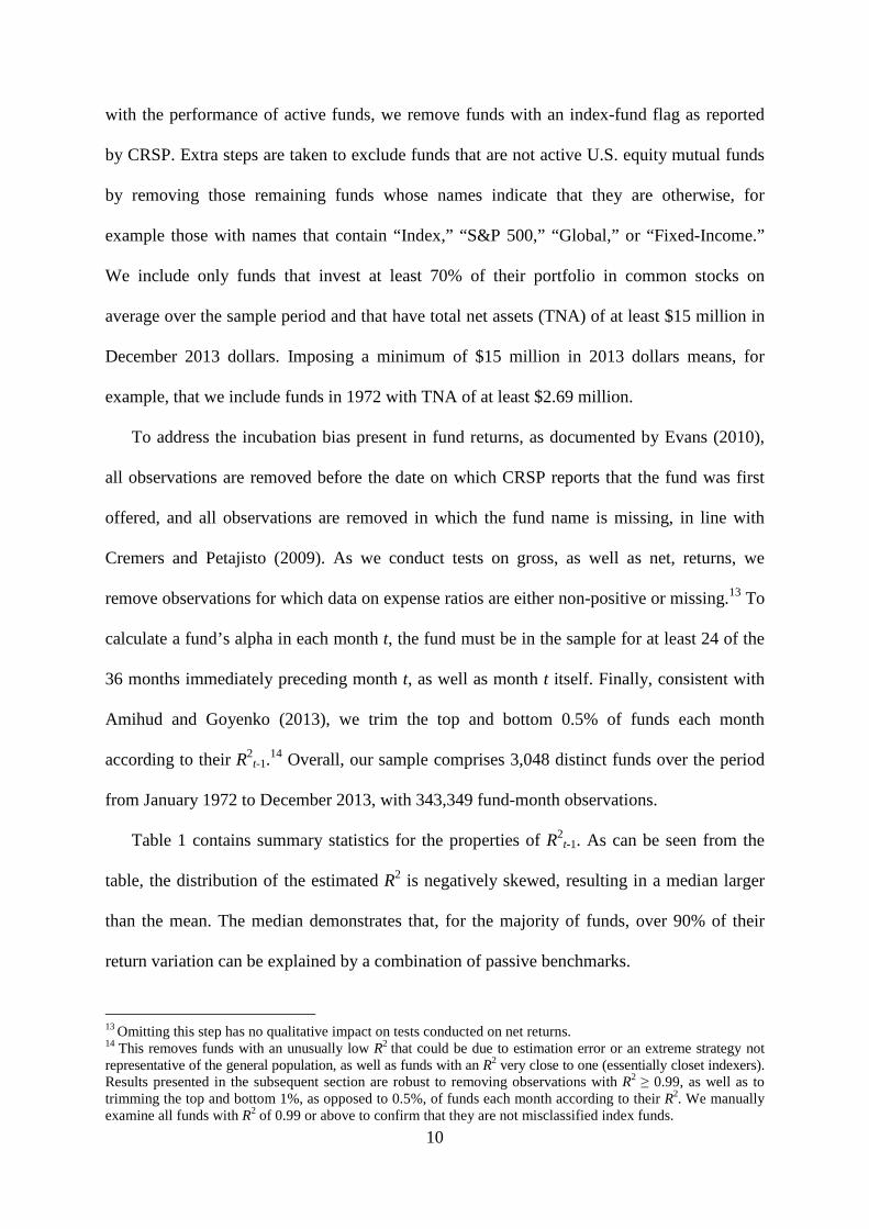
Table 1 contains summary statistics for the properties of R2t-1. As can be seen from the
table, the distribution of the estimated R2 is negatively skewed, resulting in a median larger
than the mean. The median demonstrates that, for the majority of funds, over 90% of their
return variation can be explained by a combination of passive benchmarks.
13 Omitting this step has no qualitative impact on tests conducted on net returns. 14 This removes funds with an unusually low R2 that could be due to estimation error or an extreme strategy not representative of the general population, as well as funds with an R2 very close to one (essentially closet indexers). Results presented in the subsequent section are robust to removing observations with R2 ≥ 0.99, as well as to trimming the top and bottom 1%, as opposed to 0.5%, of funds each month according to their R2. We manually examine all funds with R2 of 0.99 or above to confirm that they are not misclassified index funds.
11
Table 1. Descriptive statistics for R2t-1
This table shows descriptive statistics pertaining to the individual fund estimates of R2t-1 resulting from the four-
factor performance model of Fama-French (1993) and Carhart (1997) (FFC) over the period January 1972 to December 2013. Monthly estimates of R2
t-1 are obtained from regressions of fund returns (in excess of the one-month T bill rate) on the factors of the FFC model over the 36 months immediately preceding month t. The fund sample consists of 3,048 actively-managed U.S. equity mutual funds, with 343,349 fund-month observations.
Interpretation: R2 has a negatively skewed distribution. The median demonstrates that, for the majority of active funds, over 90% of their return variation can be explained by a combination of passive benchmarks.
Measure Mean Median Minimum Maximum
R2t-1 0.913 0.930 0.181 0.999
2.2. Cross-sectional return dispersion data
To compute cross-sectional return dispersion, historical constituent lists for the S&P 500
index are downloaded from Compustat North America and matched with return data from
CRSP using the CRSP/Compustat Merged database. Equally weighted average monthly
returns, including distributions, on S&P 500 index constituents are obtained from CRSP. The
final sample spans 504 months from January 1972 to December 2013, with 100 months in the
third dispersion quintile, and the remaining quintiles comprising 101 months each.
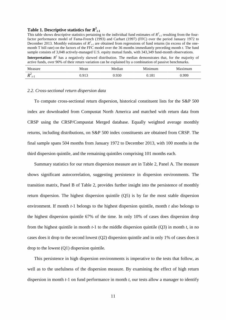
Summary statistics for our return dispersion measure are in Table 2, Panel A. The measure
shows significant autocorrelation, suggesting persistence in dispersion environments. The
transition matrix, Panel B of Table 2, provides further insight into the persistence of monthly
return dispersion. The highest dispersion quintile (Q5) is by far the most stable dispersion
environment. If month t-1 belongs to the highest dispersion quintile, month t also belongs to
the highest dispersion quintile 67% of the time. In only 10% of cases does dispersion drop
from the highest quintile in month t-1 to the middle dispersion quintile (Q3) in month t, in no
cases does it drop to the second lowest (Q2) dispersion quintile and in only 1% of cases does it
drop to the lowest (Q1) dispersion quintile.
This persistence in high dispersion environments is imperative to the tests that follow, as
well as to the usefulness of the dispersion measure. By examining the effect of high return
dispersion in month t-1 on fund performance in month t, our tests allow a manager to identify
12
the move to a high dispersion environment and react by implementing an active strategy in
the subsequent month. This means that managers do not need to predict an increase in
dispersion before it first occurs. Likewise it enables investors to observe dispersion in month
t-1 before deciding whether to invest in active funds in month t. The transition matrix shows
that there is very little risk that a manager or an investor would react to the observation of
high return dispersion in month t-1 only for dispersion to drop substantially in the subsequent
month.
Table 2. Summary statistics for cross-sectional return dispersion This table presents a summary of the statistics pertaining to our measure of monthly cross-sectional return dispersion over the period January 1972 to December 2013. Panel A presents the mean, median, standard deviation and autocorrelation of the dispersion measure, where ρ(t-1, t) denotes the first order autocorrelation of return dispersion between month t-1 and month t. Panel B presents the transition matrix of return dispersion quintiles between month t-1 and month t over the period, with figures expressed in percentages. Quintiles are formed by sorting the months of the sample period based on their level of return dispersion.
Interpretation: Return dispersion shows significant autocorrelation, and the highest dispersion quintile (Q5) is the most stable dispersion environment. This suggests that there is little risk of reacting to the observation of high dispersion in month t-1, only for dispersion to drop substantially in the subsequent month.
Panel A: Descriptive statistics for cross-sectional return dispersion
Measure Mean Median Standard deviation ρ(t-1, t)
Return dispersion 8.60% 7.93% 2.64% 0.679
Panel B: Transition matrix for cross-sectional return dispersion quintiles (%)
RD Quintile t
RD Quintile t-1 Q1 Q2 Q3 Q4 Q5
Q1 46.00 23.00 18.00 10.00 3.00
Q2 28.71 32.67 21.78 15.84 0.99
Q3 13.86 29.70 24.75 22.77 8.91
Q4 9.90 14.85 25.74 29.70 19.80
Q5 1.00 0.00 10.00 22.00 67.00
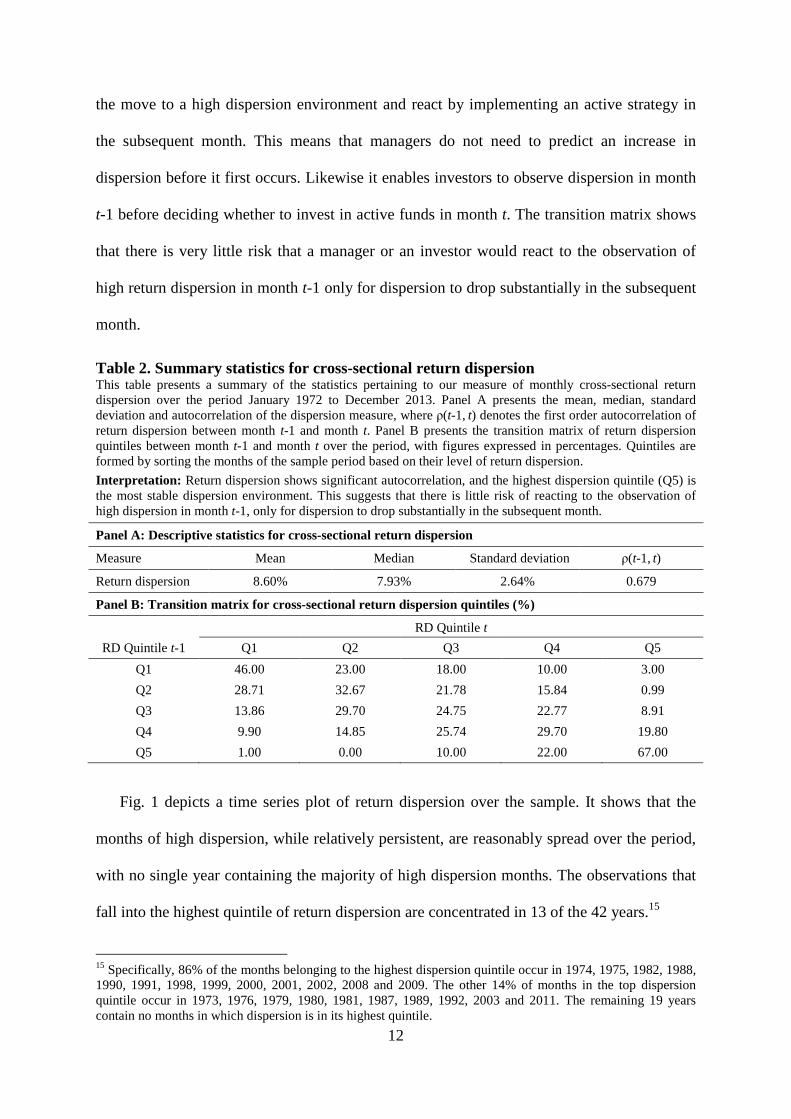
Fig. 1 depicts a time series plot of return dispersion over the sample. It shows that the
months of high dispersion, while relatively persistent, are reasonably spread over the period,
with no single year containing the majority of high dispersion months. The observations that
fall into the highest quintile of return dispersion are concentrated in 13 of the 42 years.15
15 Specifically, 86% of the months belonging to the highest dispersion quintile occur in 1974, 1975, 1982, 1988, 1990, 1991, 1998, 1999, 2000, 2001, 2002, 2008 and 2009. The other 14% of months in the top dispersion quintile occur in 1973, 1976, 1979, 1980, 1981, 1987, 1989, 1992, 2003 and 2011. The remaining 19 years contain no months in which dispersion is in its highest quintile.
13
Fig. 1. Time series plot of cross-sectional return dispersion This figure presents a time series plot of our equally weighted monthly cross-sectional return dispersion measure over the 504 months spanning January 1972 to December 2013.
Interpretation: The months of high dispersion are reasonably spread over the sample period.
3. Fund portfolio performance across dispersion environments
3.1. Return dispersion and subsequent fund performance: preliminary analysis
We begin our examination of whether the performance of funds of differing activeness is
sensitive to the return dispersion environment by analyzing average monthly returns. Each
month, we calculate the equally weighted average performance of funds in the five selectivity
portfolios. This provides a time series of monthly performance estimates for each portfolio.
Within each selectivity portfolio, estimates are then grouped according to the dispersion
quintile to which the month belongs. The equally weighted average performance for each
fund portfolio is then calculated for each of the five dispersion quintiles. Performance is first
measured using raw fund returns in excess of the market portfolio. Subsequently, we move to
examine risk-adjusted returns using FFC alphas, our main performance estimate in this study.
Table 3 reports the equally weighted average fund performance for each selectivity
portfolio over the entire sample period and for the five dispersion quintiles, where
performance is measured using excess return, defined as raw fund return in excess of a value-
weighted market portfolio comprising all NYSE, Amex and Nasdaq stocks. Standard
T-statistics are reported for each observation. Results in the bottom row (Overall) show that,
for the entire sample period, average excess return is insignificant for all funds combined.
0%
5%
10%
15%
20%
25%M
onth
ly r
etur
n di
sper
sion
Year
14
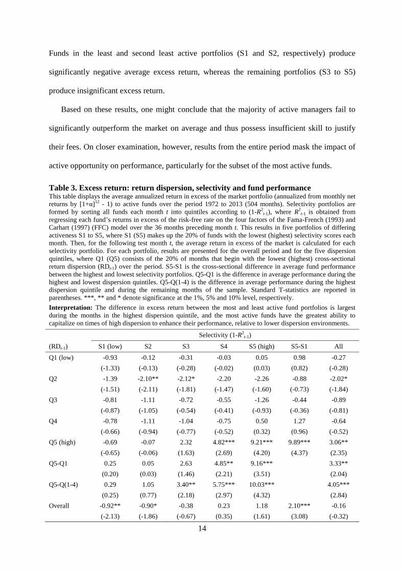
Funds in the least and second least active portfolios (S1 and S2, respectively) produce
significantly negative average excess return, whereas the remaining portfolios (S3 to S5)
produce insignificant excess return.
Based on these results, one might conclude that the majority of active managers fail to
significantly outperform the market on average and thus possess insufficient skill to justify
their fees. On closer examination, however, results from the entire period mask the impact of
active opportunity on performance, particularly for the subset of the most active funds.
Table 3. Excess return: return dispersion, selectivity and fund performance This table displays the average annualized return in excess of the market portfolio (annualized from monthly net returns by [1+α]12 - 1) to active funds over the period 1972 to 2013 (504 months). Selectivity portfolios are formed by sorting all funds each month t into quintiles according to (1-R2
t-1), where R2t-1 is obtained from
regressing each fund’s returns in excess of the risk-free rate on the four factors of the Fama-French (1993) and Carhart (1997) (FFC) model over the 36 months preceding month t. This results in five portfolios of differing activeness S1 to S5, where S1 (S5) makes up the 20% of funds with the lowest (highest) selectivity scores each month. Then, for the following test month t, the average return in excess of the market is calculated for each selectivity portfolio. For each portfolio, results are presented for the overall period and for the five dispersion quintiles, where Q1 (Q5) consists of the 20% of months that begin with the lowest (highest) cross-sectional return dispersion (RDt-1) over the period. S5-S1 is the cross-sectional difference in average fund performance between the highest and lowest selectivity portfolios. Q5-Q1 is the difference in average performance during the highest and lowest dispersion quintiles. Q5-Q(1-4) is the difference in average performance during the highest dispersion quintile and during the remaining months of the sample. Standard T-statistics are reported in parentheses. ***, ** and * denote significance at the 1%, 5% and 10% level, respectively.
Interpretation: The difference in excess return between the most and least active fund portfolios is largest during the months in the highest dispersion quintile, and the most active funds have the greatest ability to capitalize on times of high dispersion to enhance their performance, relative to lower dispersion environments.
Selectivity (1-R2t-1)
(RDt-1) S1 (low) S2 S3 S4 S5 (high) S5-S1 All
Q1 (low) -0.93 -0.12 -0.31 -0.03 0.05 0.98 -0.27
(-1.33) (-0.13) (-0.28) (-0.02) (0.03) (0.82) (-0.28)
Q2 -1.39 -2.10** -2.12* -2.20 -2.26 -0.88 -2.02*
(-1.51) (-2.11) (-1.81) (-1.47) (-1.60) (-0.73) (-1.84)
Q3 -0.81 -1.11 -0.72 -0.55 -1.26 -0.44 -0.89
(-0.87) (-1.05) (-0.54) (-0.41) (-0.93) (-0.36) (-0.81)
Q4 -0.78 -1.11 -1.04 -0.75 0.50 1.27 -0.64
(-0.66) (-0.94) (-0.77) (-0.52) (0.32) (0.96) (-0.52)
Q5 (high) -0.69 -0.07 2.32 4.82*** 9.21*** 9.89*** 3.06**
(-0.65) (-0.06) (1.63) (2.69) (4.20) (4.37) (2.35)
Q5-Q1 0.25 0.05 2.63 4.85** 9.16***
3.33**
(0.20) (0.03) (1.46) (2.21) (3.51)
(2.04)
Q5-Q(1-4) 0.29 1.05 3.40** 5.75*** 10.03***
4.05***
(0.25) (0.77) (2.18) (2.97) (4.32)
(2.84)
Overall -0.92** -0.90* -0.38 0.23 1.18 2.10*** -0.16
(-2.13) (-1.86) (-0.67) (0.35) (1.61) (3.08) (-0.32)
15
A positive relation exists between cross-sectional return dispersion and subsequent fund
performance that increases with the activeness of the fund portfolio. The difference in excess
returns between the months comprising the highest and lowest dispersion quintiles (Q5-Q1),
and between the highest dispersion quintile and the remaining months of the sample period
[Q5-Q(1-4)], are in rows six and seven, respectively. The less active fund portfolios (S1 and
S2) produce insignificant or negative excess return over the lower dispersion quintiles and are
unable to improve their performance significantly in the highest dispersion quintile. By
contrast, the three more active fund portfolios (S3 to S5) are able to produce significantly
greater excess return over the highest dispersion quintile, representing those months when
active bets have the greatest impact on returns, than that produced in other months. In
particular, the most active fund portfolio produces excess return that is 9.16% p.a. (T = 3.51)
greater during the highest dispersion quintile than during the lowest dispersion quintile, and
10.03% p.a. (T = 4.32) greater in the highest dispersion quintile than in the remaining months
of the sample combined. The most active portfolio also produces the greatest excess return
over any single dispersion quintile. Consistent with the ability to capitalize on high cross-
sectional return dispersion to generate outperformance, during the months belonging to the
highest dispersion quintile (Q5), the most active fund portfolio earns an average excess return
of 9.21% p.a. (T = 4.20).
Periods of high return dispersion are also vital to the outperformance of the most, relative
to the least, active funds, displayed in column six (S5-S1). Consistent with the findings of
Amihud and Goyenko (2013), the most active funds outperform the least active funds over
the period as a whole. Taking the analysis further, however, examination of the dispersion
environment reveals that there is no significant difference in average excess return between
the highest and lowest selectivity portfolios over any of the four lowest dispersion quintiles.
Over the highest dispersion quintile, on the other hand, a hypothetical portfolio comprising a
16
long position in the most active funds and a short position in the least active funds produces
an average excess return of 9.89% p.a. (T = 4.37).
While examination of excess returns facilitates a comparison of fund returns relative to
the overall market, it does not account for the riskiness of a fund’s strategies. We therefore
concentrate the remainder of our analysis on risk-adjusted returns, our primary measure being
alpha estimated from the four-factor FFC model. Analysis of FFC alphas provides additional
valuable insights when considering the ability of managers to exploit cross-sectional return
dispersion to generate outperformance, as the additional factors contained in the FFC model –
size, value and momentum – themselves represent cross-sectional differences in asset returns.
Measuring performance using these alphas therefore allows us to examine whether the most
active managers can capitalize on additional sources of high dispersion beyond those between
small and big stocks, value and growth stocks, and stocks with high and low past returns.
In this section, monthly alphas are estimated in two steps to mitigate look-ahead bias. In
the first, we perform rolling regressions for the FFC model, described in Eq. (3), to estimate
factor loadings using 36 months of data. We then apply the resulting model coefficients to the
subsequent month’s returns to obtain a one month alpha for each fund:
αit = Rit – Rft – bit-1(Rmt – Rft) – sit-1(SMBt) – hit-1(HMLt) – mit-1(MOMt) (4)
where αit is the alpha to fund i in month t and bit-1, sit-1, hit-1 and mit-1 are the market, size,
value and momentum factor loadings, estimated over the 36 months prior to month t.
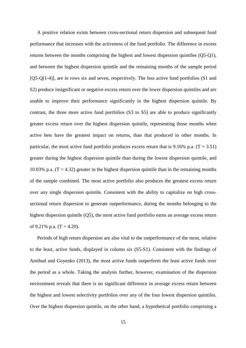
Table 4 presents equally weighted average fund FFC alphas and standard T-statistics.
While adjusting for risk reduces the size of the performance estimates, their significance and
qualitative interpretation remain. Consistent with results of excess returns, the outperformance
of the most, relative to the least, active funds is concentrated in the months comprising the
highest dispersion quintile. During these months, the most active fund portfolio produces
FFC alpha of 3.88% p.a. (T = 2.58), 4.69% p.a. (T = 3.88) higher than the least active funds.
17
In addition, the most active portfolio produces significantly greater alpha in both the highest,
relative to the lowest, dispersion quintile (5.25% p.a., T = 3.14) and the highest dispersion
quintile relative to the remaining months of the sample (5.31% p.a., T = 3.30).
Table 4. FFC alpha: return dispersion, selectivity and fund performance This table displays the average annualized Fama-French (1993) and Carhart (1997) (FFC) four-factor alpha (annualized from monthly net returns) to active funds over the period 1972 to 2013 (504 months). Selectivity portfolios are formed by sorting all funds each month t into quintiles according to (1-R2
t-1), where R2t-1 is
obtained from regressing each fund’s return in excess of the risk-free rate on the FFC factors over the 36 months prior to month t. This results in five portfolios of differing activeness S1 to S5, where S1 (S5) makes up the 20% of funds with the lowest (highest) selectivity scores each month. Then, for the following test month t, the average alpha is calculated for each selectivity portfolio. For each portfolio, results are shown for the overall period and for five dispersion quintiles, where Q1 (Q5) comprises the 20% of months that begin with the lowest (highest) return dispersion (RDt-1) over the period. S5-S1 is the cross-sectional difference in alpha between the highest and lowest selectivity portfolios. Q5-Q1 is the difference in alpha during the highest and lowest dispersion quintiles. Q5-Q(1-4) is the difference in alpha between the highest dispersion quintile and the remaining months of the sample. Standard T-statistics are reported in parentheses. ***, ** and * denote significance at the 1%, 5% and 10% level, respectively.
Interpretation: Consistent with results using excess returns (Table 3), the additional FFC alpha of the most, relative to the least, active funds is concentrated in the months comprising the top dispersion quintile, and the most active funds show the greatest improvement in alpha in times of high dispersion, relative to other months.
Selectivity (1-R2t-1)
(RDt-1) S1 (low) S2 S3 S4 S5 (high) S5-S1 All
Q1 (low) -0.97* -0.97* -1.23** -1.27** -1.38* -0.41 -1.16**
(-1.95) (-1.88) (-2.23) (-2.21) (-1.85) (-0.72) (-2.29)
Q2 -0.76 -1.16* -1.11 -1.47* -0.78 -0.03 -1.06
(-1.20) (-1.70) (-1.33) (-1.76) (-0.87) (-0.04) (-1.50)
Q3 -0.79 -1.22* -1.04 -1.78* -1.65 -0.86 -1.30*
(-1.27) (-1.67) (-1.35) (-1.94) (-1.60) (-0.91) (-1.83)
Q4 -0.54 -1.29* -1.60* -1.65 -1.66 -1.12 -1.35
(-0.83) (-1.93) (-1.88) (-1.62) (-1.14) (-0.93) (-1.61)
Q5 (high) -0.82 -0.49 0.47 1.12 3.88*** 4.69*** 0.82
(-0.94) (-0.42) (0.36) (0.80) (2.58) (3.88) (0.71)
Q5-Q1 0.15 0.49 1.70 2.39 5.25***
1.98
(0.15) (0.39) (1.20) (1.58) (3.14)
(1.58)
Q5-Q(1-4) -0.05 0.68 1.73 2.70* 5.31***
2.06*
(-0.06) (0.57) (1.26) (1.82) (3.30)
(1.70)
Overall -0.77*** -1.02*** -0.91** -1.01** -0.34 0.44 -0.81**
(-2.61) (-2.95) (-2.25) (-2.29) (-0.64) (1.00) (-2.24)
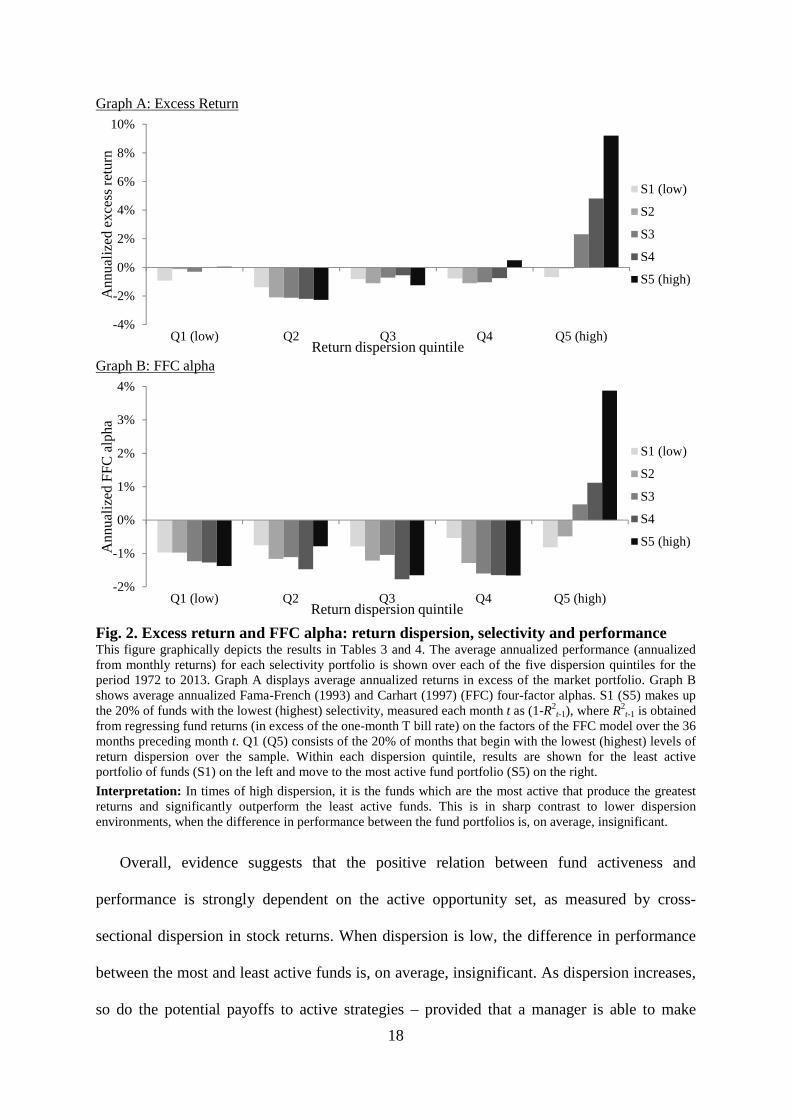
The information contained in Tables 3 and 4 is depicted graphically in Fig. 2. Excess
returns and FFC alphas are shown in Graphs A and B, respectively. Within each dispersion
quintile, results are shown for the least active portfolio of funds (S1) on the left and move to
the most active fund portfolio (S5) on the right.
18
Graph A: Excess Return
Graph B: FFC alpha
Fig. 2. Excess return and FFC alpha: return dispersion, selectivity and performance This figure graphically depicts the results in Tables 3 and 4. The average annualized performance (annualized from monthly returns) for each selectivity portfolio is shown over each of the five dispersion quintiles for the period 1972 to 2013. Graph A displays average annualized returns in excess of the market portfolio. Graph B shows average annualized Fama-French (1993) and Carhart (1997) (FFC) four-factor alphas. S1 (S5) makes up the 20% of funds with the lowest (highest) selectivity, measured each month t as (1-R2
t-1), where R2t-1 is obtained
from regressing fund returns (in excess of the one-month T bill rate) on the factors of the FFC model over the 36 months preceding month t. Q1 (Q5) consists of the 20% of months that begin with the lowest (highest) levels of return dispersion over the sample. Within each dispersion quintile, results are shown for the least active portfolio of funds (S1) on the left and move to the most active fund portfolio (S5) on the right.
Interpretation: In times of high dispersion, it is the funds which are the most active that produce the greatest returns and significantly outperform the least active funds. This is in sharp contrast to lower dispersion environments, when the difference in performance between the fund portfolios is, on average, insignificant.
Overall, evidence suggests that the positive relation between fund activeness and
performance is strongly dependent on the active opportunity set, as measured by cross-
sectional dispersion in stock returns. When dispersion is low, the difference in performance
between the most and least active funds is, on average, insignificant. As dispersion increases,
so do the potential payoffs to active strategies – provided that a manager is able to make
-4%
-2%
0%
2%
4%
6%
8%
10%
Q1 (low) Q2 Q3 Q4 Q5 (high)
Ann
ualiz
ed e
xces
s re
turn
Return dispersion quintile
S1 (low)
S2
S3
S4
S5 (high)
-2%
-1%
0%
1%
2%
3%
4%
Q1 (low) Q2 Q3 Q4 Q5 (high)
Ann
ualiz
ed F
FC
alp
ha
Return dispersion quintile
S1 (low)
S2
S3
S4
S5 (high)
19
active bets that produce positive returns. In times of high dispersion, it is the funds which are
the most active that produce the greatest returns and significantly outperform the least active
funds. The use of four-factor FFC alphas suggests that the sources of high cross-sectional
return dispersion being exploited are not restricted to those represented by the additional
factors of the FFC model. Specifically, the most active managers are able to adjust their
strategies to take advantage of sources of high return dispersion beyond those stemming from
asset size, value and momentum in returns.
3.2. Return dispersion and subsequent fund performance: gross returns
The previous examination of FFC alphas estimated from net returns tests a manager’s ability
to produce risk-adjusted returns that not only cover the costs of their trades, but also the
management costs imposed on their investors. In contrast, tests of gross returns examine
whether managers have sufficient skill in selecting stocks to produce risk-adjusted returns
that at least cover the trading costs of their strategies, before the application of expense ratios.
Gross returns are calculated by adding back expenses to monthly fund net returns, where a
fund’s monthly expenses are calculated as one-twelfth of a fund’s expense ratio in the year in
which the month belongs.
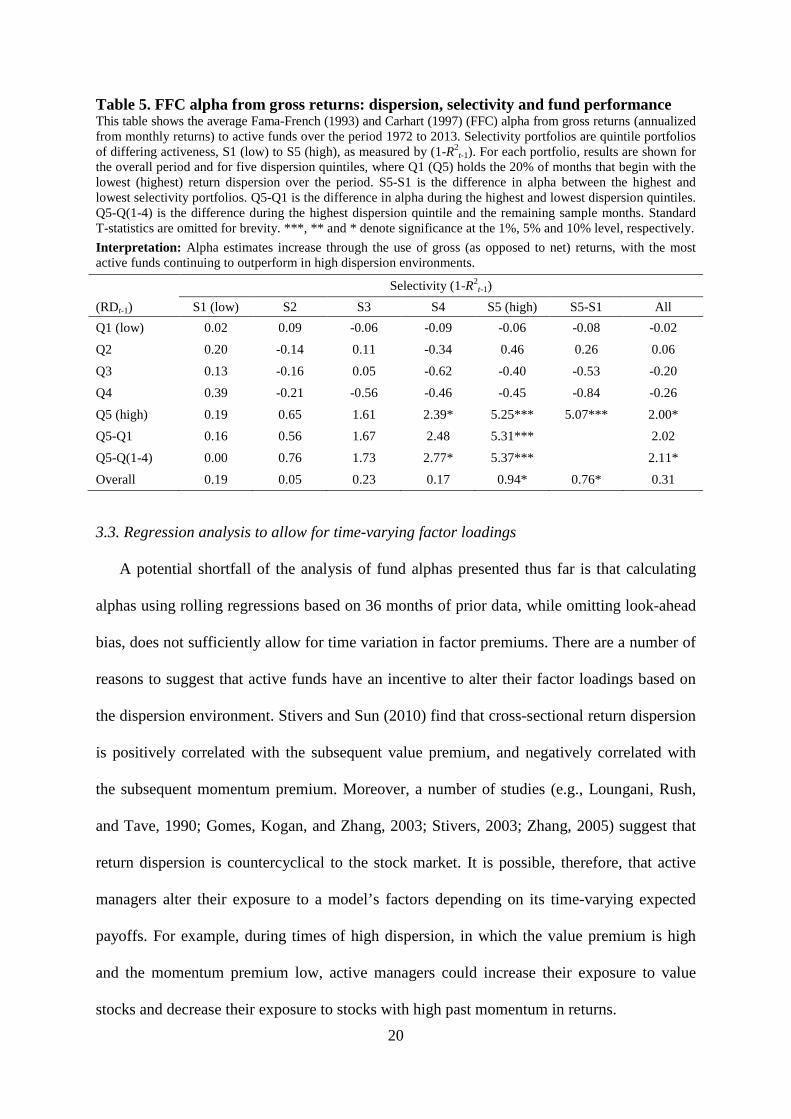
Table 5 displays the results from replicating the previous test on FFC alphas, with the
exception that alphas are estimated from gross, as opposed to net, returns. Results are consistent
with our previous findings. The difference in performance between the most and least active
fund portfolios is largest during the months belonging to the highest dispersion quintile, and the
portfolio comprising the most active funds has the greatest ability to capitalize on times of high
return dispersion to enhance its performance, relative to lower dispersion environments. In
addition, the most active funds on average produce significantly positive FFC alpha in the
highest dispersion quintile, suggesting that the stocks selected by funds in the most active
portfolio significantly outperform the market in times of high active opportunity.
20
Table 5. FFC alpha from gross returns: dispersion, selectivity and fund performance This table shows the average Fama-French (1993) and Carhart (1997) (FFC) alpha from gross returns (annualized from monthly returns) to active funds over the period 1972 to 2013. Selectivity portfolios are quintile portfolios of differing activeness, S1 (low) to S5 (high), as measured by (1-R2
t-1). For each portfolio, results are shown for the overall period and for five dispersion quintiles, where Q1 (Q5) holds the 20% of months that begin with the lowest (highest) return dispersion over the period. S5-S1 is the difference in alpha between the highest and lowest selectivity portfolios. Q5-Q1 is the difference in alpha during the highest and lowest dispersion quintiles. Q5-Q(1-4) is the difference during the highest dispersion quintile and the remaining sample months. Standard T-statistics are omitted for brevity. ***, ** and * denote significance at the 1%, 5% and 10% level, respectively.
Interpretation: Alpha estimates increase through the use of gross (as opposed to net) returns, with the most active funds continuing to outperform in high dispersion environments.
Selectivity (1-R2t-1)
(RDt-1) S1 (low) S2 S3 S4 S5 (high) S5-S1 All
Q1 (low) 0.02 0.09 -0.06 -0.09 -0.06 -0.08 -0.02
Q2 0.20 -0.14 0.11 -0.34 0.46 0.26 0.06
Q3 0.13 -0.16 0.05 -0.62 -0.40 -0.53 -0.20
Q4 0.39 -0.21 -0.56 -0.46 -0.45 -0.84 -0.26
Q5 (high) 0.19 0.65 1.61 2.39* 5.25*** 5.07*** 2.00*
Q5-Q1 0.16 0.56 1.67 2.48 5.31***
2.02
Q5-Q(1-4) 0.00 0.76 1.73 2.77* 5.37***
2.11*
Overall 0.19 0.05 0.23 0.17 0.94* 0.76* 0.31
3.3. Regression analysis to allow for time-varying factor loadings
A potential shortfall of the analysis of fund alphas presented thus far is that calculating
alphas using rolling regressions based on 36 months of prior data, while omitting look-ahead
bias, does not sufficiently allow for time variation in factor premiums. There are a number of
reasons to suggest that active funds have an incentive to alter their factor loadings based on
the dispersion environment. Stivers and Sun (2010) find that cross-sectional return dispersion
is positively correlated with the subsequent value premium, and negatively correlated with
the subsequent momentum premium. Moreover, a number of studies (e.g., Loungani, Rush,
and Tave, 1990; Gomes, Kogan, and Zhang, 2003; Stivers, 2003; Zhang, 2005) suggest that
return dispersion is countercyclical to the stock market. It is possible, therefore, that active
managers alter their exposure to a model’s factors depending on its time-varying expected
payoffs. For example, during times of high dispersion, in which the value premium is high
and the momentum premium low, active managers could increase their exposure to value
stocks and decrease their exposure to stocks with high past momentum in returns.
21
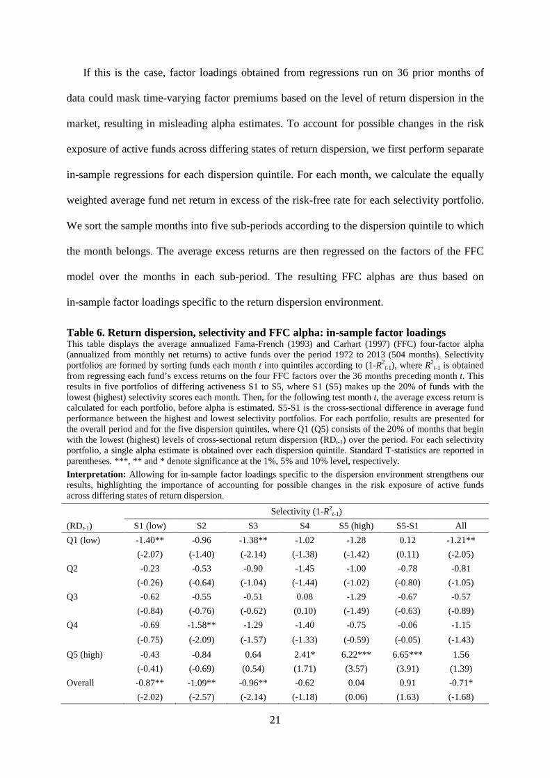
If this is the case, factor loadings obtained from regressions run on 36 prior months of
data could mask time-varying factor premiums based on the level of return dispersion in the
market, resulting in misleading alpha estimates. To account for possible changes in the risk
exposure of active funds across differing states of return dispersion, we first perform separate
in-sample regressions for each dispersion quintile. For each month, we calculate the equally
weighted average fund net return in excess of the risk-free rate for each selectivity portfolio.
We sort the sample months into five sub-periods according to the dispersion quintile to which
the month belongs. The average excess returns are then regressed on the factors of the FFC
model over the months in each sub-period. The resulting FFC alphas are thus based on
in-sample factor loadings specific to the return dispersion environment.
Table 6. Return dispersion, selectivity and FFC alpha: in-sample factor loadings This table displays the average annualized Fama-French (1993) and Carhart (1997) (FFC) four-factor alpha (annualized from monthly net returns) to active funds over the period 1972 to 2013 (504 months). Selectivity portfolios are formed by sorting funds each month t into quintiles according to (1-R2
t-1), where R2t-1 is obtained
from regressing each fund’s excess returns on the four FFC factors over the 36 months preceding month t. This results in five portfolios of differing activeness S1 to S5, where S1 (S5) makes up the 20% of funds with the lowest (highest) selectivity scores each month. Then, for the following test month t, the average excess return is calculated for each portfolio, before alpha is estimated. S5-S1 is the cross-sectional difference in average fund performance between the highest and lowest selectivity portfolios. For each portfolio, results are presented for the overall period and for the five dispersion quintiles, where Q1 (Q5) consists of the 20% of months that begin with the lowest (highest) levels of cross-sectional return dispersion (RDt-1) over the period. For each selectivity portfolio, a single alpha estimate is obtained over each dispersion quintile. Standard T-statistics are reported in parentheses. ***, ** and * denote significance at the 1%, 5% and 10% level, respectively.
Interpretation: Allowing for in-sample factor loadings specific to the dispersion environment strengthens our results, highlighting the importance of accounting for possible changes in the risk exposure of active funds across differing states of return dispersion.
Selectivity (1-R2t-1)
(RDt-1) S1 (low) S2 S3 S4 S5 (high) S5-S1 All
Q1 (low) -1.40** -0.96 -1.38** -1.02 -1.28 0.12 -1.21**
(-2.07) (-1.40) (-2.14) (-1.38) (-1.42) (0.11) (-2.05)
Q2 -0.23 -0.53 -0.90 -1.45 -1.00 -0.78 -0.81
(-0.26) (-0.64) (-1.04) (-1.44) (-1.02) (-0.80) (-1.05)
Q3 -0.62 -0.55 -0.51 0.08 -1.29 -0.67 -0.57
(-0.84) (-0.76) (-0.62) (0.10) (-1.49) (-0.63) (-0.89)
Q4 -0.69 -1.58** -1.29 -1.40 -0.75 -0.06 -1.15
(-0.75) (-2.09) (-1.57) (-1.33) (-0.59) (-0.05) (-1.43)
Q5 (high) -0.43 -0.84 0.64 2.41* 6.22*** 6.65*** 1.56
(-0.41) (-0.69) (0.54) (1.71) (3.57) (3.91) (1.39)
Overall -0.87** -1.09** -0.96** -0.62 0.04 0.91 -0.71*
(-2.02) (-2.57) (-2.14) (-1.18) (0.06) (1.63) (-1.68)
22
As can be seen in Table 6, our findings strengthen after allowing for time-varying factor
loadings. Consistent with the preceding analysis, the most active fund portfolio produces
significantly positive FFC alpha during the highest dispersion quintile. However the
magnitude of this performance is now higher: 6.22% p.a. (T = 3.57) compared to 3.88% p.a.
(T = 2.58) when using 36 month rolling regressions in Table 4. The outperformance of the
most, relative to the least, active portfolio, which remains concentrated in times of elevated
dispersion, is 6.65% p.a. (T = 3.91) during the highest dispersion quintile, again exceeding
the 4.69% p.a. (T = 3.88) difference in FFC alpha when rolling regressions are used.
In a further check, we assess the difference in fund performance produced over the
highest dispersion quintile, relative to the remaining months of the sample, by performing
indicator regressions that allow factor loadings to change depending on whether a month
belongs to the highest return dispersion quintile. Specifically, we construct a dummy variable
equal to one if the month is part of the highest dispersion quintile over our sample, and zero
otherwise. For each selectivity portfolio, we then re-run the regression in Eq. (3) on net
returns over the sample period as a whole, adding the high dispersion indicator, as well as the
cross-products of the indicator and the factors of the FFC model.
Table 7 displays the results of the indicator regression analysis. The equally weighted
average annualized alpha produced during months in the low to medium dispersion quintiles
(dispersion quintiles one through four) is displayed in the top row. The difference in alpha
between months in the highest dispersion quintile and the remaining months of the sample is
represented by the ordinary least squares alpha coefficient associated with the high dispersion
indicator in the second row [Alpha*DV(Q5t-1)]. Standard T-statistics are displayed in
parentheses. Because dispersion environments can be relatively persistent, spurious
correlation in the high dispersion indicator can lead to incorrect inferences based on standard
T-statistics. To compensate, we adjust the critical value cut-offs according to the method
23
outlined in Powell et al. (2009). Based on the properties of the data, the cut-off T-statistic is
(-2.03/2.08) for significance at the 5% level.
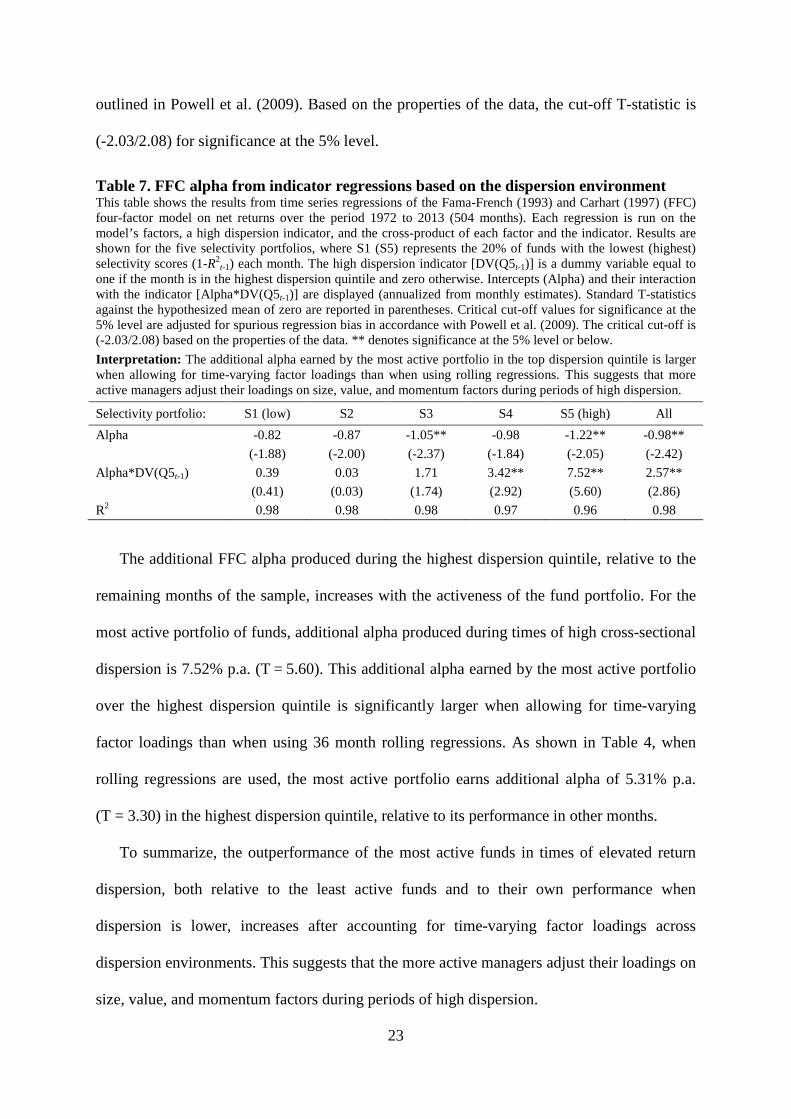
Table 7. FFC alpha from indicator regressions based on the dispersion environment This table shows the results from time series regressions of the Fama-French (1993) and Carhart (1997) (FFC) four-factor model on net returns over the period 1972 to 2013 (504 months). Each regression is run on the model’s factors, a high dispersion indicator, and the cross-product of each factor and the indicator. Results are shown for the five selectivity portfolios, where S1 (S5) represents the 20% of funds with the lowest (highest) selectivity scores (1-R2
t-1) each month. The high dispersion indicator [DV(Q5t-1)] is a dummy variable equal to one if the month is in the highest dispersion quintile and zero otherwise. Intercepts (Alpha) and their interaction with the indicator [Alpha*DV(Q5t-1)] are displayed (annualized from monthly estimates). Standard T-statistics against the hypothesized mean of zero are reported in parentheses. Critical cut-off values for significance at the 5% level are adjusted for spurious regression bias in accordance with Powell et al. (2009). The critical cut-off is (-2.03/2.08) based on the properties of the data. ** denotes significance at the 5% level or below.
Interpretation: The additional alpha earned by the most active portfolio in the top dispersion quintile is larger when allowing for time-varying factor loadings than when using rolling regressions. This suggests that more active managers adjust their loadings on size, value, and momentum factors during periods of high dispersion.
Selectivity portfolio: S1 (low) S2 S3 S4 S5 (high) All
Alpha -0.82 -0.87 -1.05** -0.98 -1.22** -0.98**
(-1.88) (-2.00) (-2.37) (-1.84) (-2.05) (-2.42)
Alpha*DV(Q5t-1) 0.39 0.03 1.71 3.42** 7.52** 2.57**
(0.41) (0.03) (1.74) (2.92) (5.60) (2.86)
R2 0.98 0.98 0.98 0.97 0.96 0.98
The additional FFC alpha produced during the highest dispersion quintile, relative to the
remaining months of the sample, increases with the activeness of the fund portfolio. For the
most active portfolio of funds, additional alpha produced during times of high cross-sectional
dispersion is 7.52% p.a. (T = 5.60). This additional alpha earned by the most active portfolio
over the highest dispersion quintile is significantly larger when allowing for time-varying
factor loadings than when using 36 month rolling regressions. As shown in Table 4, when
rolling regressions are used, the most active portfolio earns additional alpha of 5.31% p.a.
(T = 3.30) in the highest dispersion quintile, relative to its performance in other months.
To summarize, the outperformance of the most active funds in times of elevated return
dispersion, both relative to the least active funds and to their own performance when
dispersion is lower, increases after accounting for time-varying factor loadings across
dispersion environments. This suggests that the more active managers adjust their loadings on
size, value, and momentum factors during periods of high dispersion.

24
3.4. Selectivity deciles
The preceding analysis concentrates on evaluating performance across funds sorted into
quintile portfolios according to their selectivity. The use of quintiles is consistent with the
existing literature on fund activeness (e.g., Cremers and Petajisto, 2009; Amihud and
Goyenko, 2013), facilitating a more direct comparison with prior findings.
Nonetheless, if the degree of activeness is an indication of a manager’s ability to produce
alpha, it is possible that the use of quintile portfolios could result in the retention of managers
with lower stock-picking ability at the margin, thereby diluting results for the most active
funds. In this section, we therefore repeat the analysis outlined in Sections 3.1 and 3.3, but
sort funds each month into decile portfolios according to their selectivity scores.
Table A.1 in the Appendix presents results for the two least (S1 and S2) and most (S9 and
S10) active decile portfolios. Panel A shows results from rolling regressions, as reported for
selectivity quintiles in Table 4. Panels B and C show results from the in-sample and indicator
regressions reported for quintiles in Tables 6 and 7, respectively.
In all tests, the two most active decile portfolios produce alpha of similar sizes during
times of elevated dispersion. To illustrate, when rolling regressions are used, portfolio S10
produces alpha of 3.86% p.a. (T = 2.61) during the top dispersion months and portfolio S9
produces alpha of 3.88% p.a. (T = 2.30) in these times (Table A.1, Panel A). When using
indicator regressions (Panel C), S10 is able to produce 7.56% p.a. (T = 4.99) greater alpha in
times of high dispersion, relative to lower dispersion environments, whereas S9 produces
additional alpha of 7.44% p.a. (T = 5.24). This suggests that, within the subset of the most
active funds, higher activeness at the margin does not necessarily lead to greater
outperformance. As such, further segregating the most active fund quintile is not required to
filter out value-destroying managers. We therefore focus the remainder of our analysis on
quintile portfolios for consistency with existing literature.

25
3.5. The impact of return dispersion in a multivariate regression
To control for the impact of fund-level characteristics on fund performance, we conduct a
panel regression of fund alpha on lagged, fund-level explanatory variables along with our
high dispersion indicator employed in Section 3.3:
alphai,t = a0 + a1DV(Q5t-1) + a2selectivityi,t-1 + a3[selectivityi,t-1*DV(Q5t-1)]
+ a4Xi,t-1 + ei,t (5)
where alphai,t is calculated using the FFC model in Eq. (4), DV(Q5t-1) is a dummy variable
equal to one if dispersion in month t-1 is in the top 20% over the sample period, and zero
otherwise, and selectivityi,t-1 is calculated as (1-R2i,t-1), as outlined in Section 1.2. Xi,t-1 is a
vector of one-month lagged, fund-specific control variables consistent with Amihud and
Goyenko (2013), including expenses (the expense ratio, in % per year), turnover (the
minimum of aggregated sales or aggregated purchases of securities, divided by the average
12-month fund TNA, in % per year), log(TNA), log(TNA)2, log(fund age), log(manager
tenure) and alpha. Alphas are annualized and expressed as percentages. Each month we
include those funds with information on all variables, resulting in a sample of 2,662 funds,
with 263,474 fund-month observations. We include style fixed effects, and heteroskedasticity
and autocorrelation consistent standard errors clustered by fund.
Our primary coefficient of interest is a3. Consistent with our prior findings, we expect the
relation between fund activeness and performance to be significantly stronger during months
of high dispersion. That is, we expect a3 to be positive. As can be seen in the first column of
Table 8, a3 is large and significantly positive at 14.831 (T = 5.61). To illustrate, this suggests
that, controlling for the other variables, a 10% increase in selectivity during the months in the
highest dispersion quintile is associated with a 1.48% increase in annualized FFC alpha.
When lagged alpha is excluded from the regression (column two), a3 increases to 16.246
(T = 5.96). This is because, with the persistence of activeness between months, a fund with
higher selectivity in month t-1 is also likely to have higher alpha in month t-1. The inclusion
26
of alphai,t-1 therefore partly absorbs the effect of selectivity on performance. Further, while a2
(the coefficient on selectivityi,t-1) is significantly negative when alphai,t-1 is included, a2 loses
significance when alphai,t-1 is excluded. This suggests that the positive relation between
activeness and FFC alpha is isolated to the months in the highest dispersion quintile over the
sample, but also that higher activity does not necessarily destroy value in other months.
Columns three and four show the same regressions as columns one and two, respectively,
except that observations are only included if the manager has been in place for at least 36
months. As we calculate selectivity through estimating the FFC model over the 36 months
preceding month t, if our regression is picking up the effect of manager specific skill this
should strengthen our results. In line with this, a3 increases when this requirement is imposed.
In further tests, we adjust the panel regression in Eq. (5), removing alphai,t-1 as a control
variable and replacing the dependent variable alphai,t with the Characteristic Selectivity (CS)
and Characteristic Timing (CT) measures of Daniel et al. (1997). Due to data availability, the
period examined spans January 1981 to December 2012, with 2,305 funds and 226,696 fund-
month observations.16 The use of CS and CT has two distinct advantages. Unlike alpha, the
measures are calculated directly from fund portfolio holdings and thus do not suffer from
potential bias caused by time-varying factor loadings across dispersion environments. In
addition, decomposing return into CS and CT provides insight into the source of any
outperformance in times of high dispersion.
If more active managers are able to capitalize on high cross-sectional dispersion to select
the better performing stocks, a3 should be significantly positive when CS is the dependent
variable. However, such a relation would not necessarily be expected for CT, which is based
16 Data on the Daniel, Grinblatt, Titman, and Wermers (1997) (DGTW) benchmarks and stock assignments are available from http://terpconnect.umd.edu/~wermers/ftpsite/Dgtw/coverpage.htm. These data are combined with fund holdings from Thomson Reuters CDA/Spectrum and stock returns from CRSP. Fund holdings are available from 1979. As the calculation of CT requires holdings data 13 months prior to month t, the first full year with available data is 1981. As DGTW benchmark data end in 2012, the sample period spans January 1981 to December 2012. The CS and CT measures are used by Daniel et al. (1997), Wermers (2003b) and Amihud and Goyenko (2013), among others.

27
on market timing. Columns five and six of Table 8 provide the results. Indeed, when CSi,t is
the dependent variable (column five), a3 is positive and significant at 13.927 (T = 4.11).
However a3 loses significance when the dependent variable is changed to CTi,t (column six).
Table 8: Dispersion, selectivity and fund performance: multivariate panel regressions This table displays results from multivariate panel regressions. In columns one to four, the dependent variable is fund alpha in month t, estimated from the Fama-French (1993) and Carhart (1997) (FFC) model, and regressions are performed over the period 1972 to 2013 (504 months). The first two columns show results from the full fund sample. Columns three and four show results from a sample restricted to observations with manager tenure of at least three years. The dependent variables in columns five and six are the month t “Characteristic Selectivity” (CS) and “Characteristic Timing” (CT) measures of Daniel et al. (1997). In these columns, the regressions are performed over the period January 1981 to December 2012 (384 months). Alpha, CS and CT are annualized and expressed in percentage points. All control variables are measured at the end of month t-1. DV(Q5t-1) is an indicator variable equal to one if return dispersion at the end of month t-1 is in the top 20% over the period, and zero otherwise. Selectivityi,t-1 is calculated as (1-R2
i,t-1), estimated from regressions of the FFC model over the 36 months preceding month t. Alphai,t-1 is the intercept from the same regression. Expenses and turnover are annual values, expressed as percentages. Fund age and manager tenure are measured in years. Style dummy variables are included in the regression. T-statistics are based on heteroskedasticity and autocorrelation consistent standard errors clustered by fund. ***, ** and * denote significance at the 1%, 5% and 10% level, respectively.
Interpretation: After controlling for fund-level characteristics, the positive relation between fund selectivity and performance (as measured by either FFC alpha or CS) is considerably more pronounced during the months belonging to the highest dispersion quintile, relative to the remaining months of the sample period.
Alphai,t Alphai,t Alphai,t Alphai,t CSi,t CTi,t
DV(Q5t-1) -0.849***
(-3.67)
-0.768***
(-3.20)
-0.781***
(-2.96)
-0.721***
(-2.65)
3.357***
(10.84)
0.728***
(4.23)
Selectivityi,t-1 -1.987**
(-1.96)
-0.834
(-0.78)
-2.450**
(-2.20)
-1.266
(-1.07)
5.423***
(5.04)
0.079
(0.12)
Selectivityi,t-1*DV(Q5 t-1) 14.831*** (5.61)
16.246*** (5.96)
16.392*** (5.43)
17.986*** (5.81)
13.927*** (4.11)
1.692 (0.96)
Expensesi,t-1 -1.094***
(-5.41)
-1.279***
(-5.93)
-1.254***
(-5.20)
-1.430***
(-5.60)
0.483
(1.60)
-0.298***
(-2.76)
Turnoveri,t-1 -0.001***
(-3.94)
-0.001***
(-4.36)
-0.001***
(-3.80)
-0.001***
(-4.21)
0.001
(1.24)
-0.001
(-0.34)
log(TNAi,t-1) -0.940** (-2.25)
-0.583 (-1.36)
-0.959* (-1.93)
-0.603 (-1.20)
-2.036*** (-3.24)
0.471* (1.66)
[log(TNAi,t-1)]2 0.123
(1.50)
0.084
(1.00)
0.129
(1.32)
0.090
(0.91)
0.402***
(3.30)
-0.099*
(-1.86)
log(fund agei,t-1) 0.054
(0.39)
-0.125
(-0.82)
0.169
(0.95)
0.052
(0.27)
-0.348*
(-1.83)
-0.403***
(-3.42)
log(manager tenurei,t-1) 0.011
(0.08)
0.180
(1.30)
-0.106
(-0.42)
-0.158
(-0.57)
-0.231
(-1.32)
0.049
(0.46)
Alphai,t-1 0.170***
(11.18)
0.169***
(9.78)
Constant 0.385
(0.43)
-0.503
(-0.51)
0.991
(0.91)
0.250
(0.21)
7.126***
(5.62)
1.418**
(2.31)
Manager tenure restriction No No Yes Yes No No
Sample period 1972-2013 1972-2013 1972-2013 1972-2013 1981-2012 1981-2012
28
We conclude that, after controlling for fund-level characteristics, the positive relation
between fund activeness and performance is considerably more pronounced during the
months belonging to the highest dispersion quintile, relative to the remaining months of the
sample period. Further, the capacity of highly active managers to outperform in times of high
dispersion stems from their ability to select those stocks that go on to realize superior returns.
4. Pervasiveness and robustness tests
In this section we consider a range of alternative measures to test the robustness of our
results. Specifically, we consider alternative measures of return dispersion, fund performance
and activeness, as well as applying our tests to sub-periods within the sample.
Our primary measure of cross-sectional return dispersion, used in the preceding tests, is
the equally weighted dispersion of S&P 500 constituent stocks. The S&P 500 index is chosen
as the universe in which to calculate dispersion as it is the most commonly cited benchmark for
active funds over our sample. It is also the most popular choice for passive fund investment; for
example, close to 50% of domestic U.S. index mutual fund assets were invested in funds that
track the S&P 500 in 2013.17 As such, it represents the most frequent yardstick against which
the performance of active managers is compared, as well as the most common alternative to
active fund investment.
One potential disadvantage of isolating the measure to S&P 500 constituents, however, is
that while the index serves as the most commonly cited fund benchmark, active fund managers
are likely to have the flexibility within their mandate to invest outside of it. Therefore, our
primary measure may not fully represent the dispersion within the investible universe of active
funds. In addition, our primary dispersion measure is equally weighted to reflect that, unlike
many passive mandates, active managers are not constrained to invest in stocks according to
market capitalization weights. However, if high dispersion is concentrated in smaller stocks it
17 2014 Investment Company Fact Book, http://www.icifactbook.org/.
29
may not be fully exploitable due to price impact, and yet an equally weighted measure treats
small and large stocks as equivalent. Although this risk is mitigated within the S&P 500 index,
as its constituents are the largest 500 stocks listed on the NYSE or Nasdaq according to market
capitalization, the possibility cannot be ignored. In this section, therefore, we consider three
alternative specifications of our return dispersion measure: the value-weighted return dispersion
of S&P 500 index constituents, and both the equally weighted and value-weighted return
dispersions of a broader universe of all stocks listed on the NYSE, Amex or Nasdaq.
Further, in addition to our main measure of fund performance (FFC alpha) we also consider
alpha estimated from the CPZ four-factor model. This model contains the same conceptual
factors as FFC, but the market, size and value factors are constructed using replicable market
indexes, as opposed to the market universe of all NYSE, Amex and Nasdaq stocks and the
factor mimicking portfolios of the FFC model.18 In our tests using CPZ alpha, we calculate
selectivity using rolling regressions of the CPZ model based on 36 months of data:
Rit – Rft = ait + bit ( PSmtR & – Rft) + sit (Sizet) + hit (Valuet) + mit (MOMt) + eit (6)
where PSmtR & is the month t return on the S&P 500 index, Sizet is the month t return on the
Russell 2000 index minus the return on the S&P 500 index, and Valuet is the month t return
on the Russell 3000 Value index minus the return on the Russell 3000 Growth index,
obtained from Antti Petajisto’s website.19 All other variables are as specified in Eq. (3). As
data for the CPZ factors are only available from 1979, and calculation of R2t-1 requires data
for at least 24 of the 36 prior months, the period examined under the CPZ model spans
January 1981 to December 2013, with 3,047 funds and 329,460 fund-month observations.
18 Cremers, Petajisto, and Zitzewitz (2013) argue that the Fama and French (1993) and FFC models suffer biases as they produce non-zero alpha for passive benchmark indexes. The authors suggest an alteration to correct the issue, in which the size and value factors are based on common and tradeable benchmark indexes. The CPZ model is used in a number of studies, e.g., Da, Gao, and Jagannathan (2011), Amihud and Goyenko (2013) and Dong, Feng, and Sadka (2014). 19 Available from http://www.petajisto.net/data.html until February 2011. For the remainder of the sample, we construct the factors using total return data for the relevant indexes, obtained from Thomson Reuters Datastream.
30
We also consider whether results are robust to dividing our sample period into two
sub-samples of equal length: 1972 to 1992 and 1993 to 2013.20 Finally, we consider an
alternative measure of fund activeness, specifically the Active Share measure of Cremers and
Petajisto (2009). Results using Active Share are presented for all tests in Section 4.4.
4.1. Return dispersion and alpha calculated from rolling regressions: robustness evidence
Table 9 displays a snapshot of the key variables of interest in Table 4. In particular, it
reports the performance of the most active fund portfolio (S5) in the highest dispersion
quintile (Q5); the difference in alpha produced by the most active portfolio between the
months comprising the highest and lowest dispersion quintiles (Q5-Q1), and between the
highest dispersion quintile and the remaining months of the sample [Q5-Q(1-4)]; and the
relative performance of the most and least active fund portfolios (S5-S1) during the highest
dispersion quintile. Each panel displays a different combination of measures of dispersion,
fund alphas and sample periods.
Results across the panels are qualitatively consistent with those in Table 4. Regardless of
the dispersion metric, performance measure or sample period, the most active fund portfolio is
able to improve its performance in the highest dispersion quintile, relative to its performance
in other months. In addition, the outperformance of the most, relative to the least, active
portfolio is concentrated in the months of the top dispersion quintile. Alphas are lowest when
dispersion is constructed as an equally weighted measure using all NYSE, Amex or Nasdaq
stocks (Panel B), consistent with our prior conjecture that high dispersion among smaller
stocks may not be sufficiently exploitable. However, results using this dispersion metric
improve in subsequent tests (Tables 10 to 12). When rolling regressions are used, results from
sub-period analysis (Panels E and F) fall in significance relative to the overall sample period
20 In further unreported tests, we also find that our results do not rely on extreme levels of return dispersion in a small number of months, as they remain consistent after removing the 5% of total months with the highest or lowest levels of dispersion over the sample period.
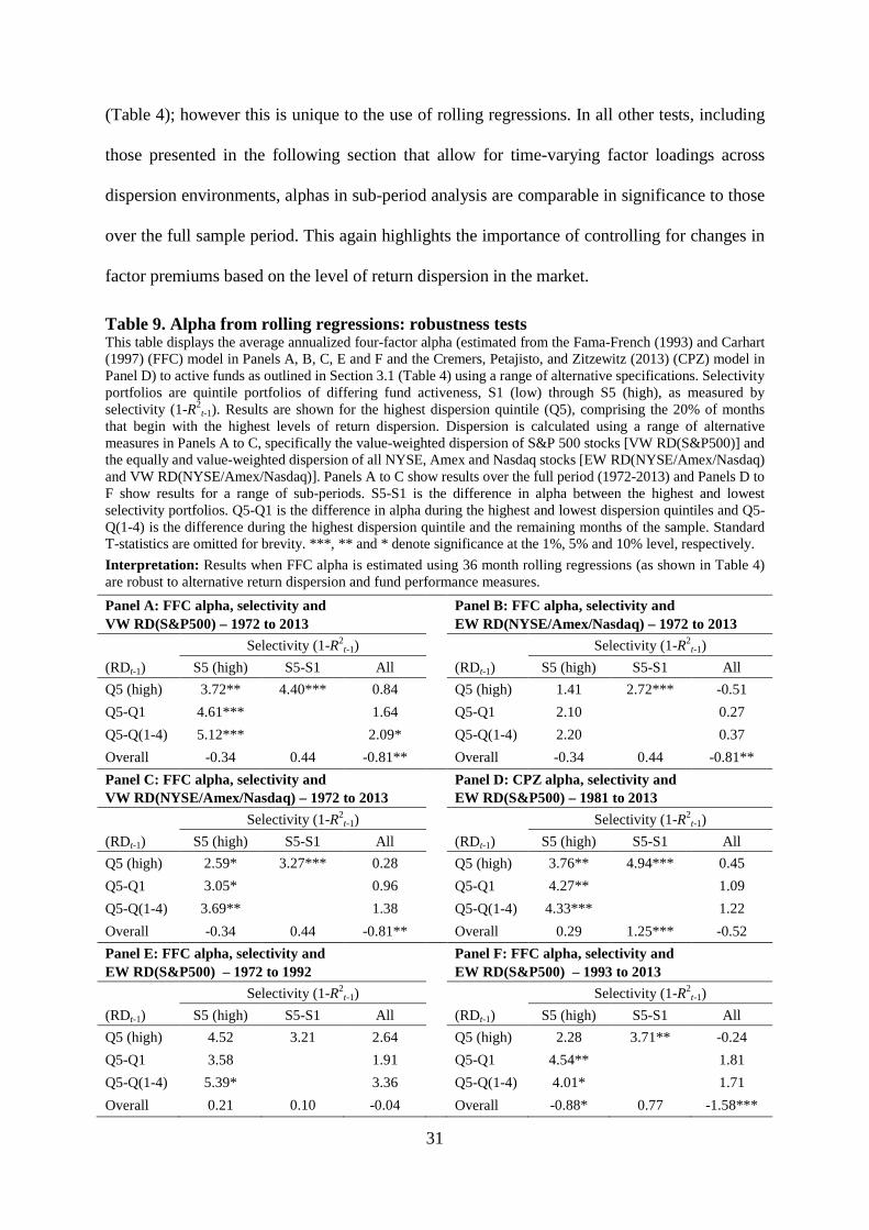
31
(Table 4); however this is unique to the use of rolling regressions. In all other tests, including
those presented in the following section that allow for time-varying factor loadings across
dispersion environments, alphas in sub-period analysis are comparable in significance to those
over the full sample period. This again highlights the importance of controlling for changes in
factor premiums based on the level of return dispersion in the market.
Table 9. Alpha from rolling regressions: robustness tests This table displays the average annualized four-factor alpha (estimated from the Fama-French (1993) and Carhart (1997) (FFC) model in Panels A, B, C, E and F and the Cremers, Petajisto, and Zitzewitz (2013) (CPZ) model in Panel D) to active funds as outlined in Section 3.1 (Table 4) using a range of alternative specifications. Selectivity portfolios are quintile portfolios of differing fund activeness, S1 (low) through S5 (high), as measured by selectivity (1-R2
t-1). Results are shown for the highest dispersion quintile (Q5), comprising the 20% of months that begin with the highest levels of return dispersion. Dispersion is calculated using a range of alternative measures in Panels A to C, specifically the value-weighted dispersion of S&P 500 stocks [VW RD(S&P500)] and the equally and value-weighted dispersion of all NYSE, Amex and Nasdaq stocks [EW RD(NYSE/Amex/Nasdaq) and VW RD(NYSE/Amex/Nasdaq)]. Panels A to C show results over the full period (1972-2013) and Panels D to F show results for a range of sub-periods. S5-S1 is the difference in alpha between the highest and lowest selectivity portfolios. Q5-Q1 is the difference in alpha during the highest and lowest dispersion quintiles and Q5-Q(1-4) is the difference during the highest dispersion quintile and the remaining months of the sample. Standard T-statistics are omitted for brevity. ***, ** and * denote significance at the 1%, 5% and 10% level, respectively.
Interpretation: Results when FFC alpha is estimated using 36 month rolling regressions (as shown in Table 4) are robust to alternative return dispersion and fund performance measures.
Panel A: FFC alpha, selectivity and VW RD(S&P500) – 1972 to 2013
Panel B: FFC alpha, selectivity and EW RD(NYSE/Amex/Nasdaq) – 1972 to 2013
Selectivity (1-R2t-1) Selectivity (1-R2
t-1)
(RDt-1) S5 (high) S5-S1 All (RDt-1) S5 (high) S5-S1 All
Q5 (high) 3.72** 4.40*** 0.84 Q5 (high) 1.41 2.72*** -0.51
Q5-Q1 4.61*** 1.64 Q5-Q1 2.10 0.27
Q5-Q(1-4) 5.12*** 2.09* Q5-Q(1-4) 2.20 0.37
Overall -0.34 0.44 -0.81** Overall -0.34 0.44 -0.81**
Panel C: FFC alpha, selectivity and VW RD(NYSE/Amex/Nasdaq) – 1972 to 2013
Panel D: CPZ alpha, selectivity and EW RD(S&P500) – 1981 to 2013
Selectivity (1-R2t-1) Selectivity (1-R2
t-1)
(RDt-1) S5 (high) S5-S1 All (RDt-1) S5 (high) S5-S1 All
Q5 (high) 2.59* 3.27*** 0.28 Q5 (high) 3.76** 4.94*** 0.45
Q5-Q1 3.05* 0.96 Q5-Q1 4.27** 1.09
Q5-Q(1-4) 3.69** 1.38 Q5-Q(1-4) 4.33*** 1.22
Overall -0.34 0.44 -0.81** Overall 0.29 1.25*** -0.52
Panel E: FFC alpha, selectivity and EW RD(S&P500) – 1972 to 1992
Panel F: FFC alpha, selectivity and EW RD(S&P500) – 1993 to 2013
Selectivity (1-R2t-1) Selectivity (1-R2
t-1)
(RDt-1) S5 (high) S5-S1 All (RDt-1) S5 (high) S5-S1 All
Q5 (high) 4.52 3.21 2.64 Q5 (high) 2.28 3.71** -0.24
Q5-Q1 3.58 1.91 Q5-Q1 4.54** 1.81
Q5-Q(1-4) 5.39* 3.36 Q5-Q(1-4) 4.01* 1.71
Overall 0.21 0.10 -0.04 Overall -0.88* 0.77 -1.58***

32
4.2. Regression analysis to allow for time-varying factor loadings: robustness evidence
Table 10 shows results of the robustness tests on the regressions performed within each
dispersion quintile, as outlined in Section 3.3 and reported in Table 6. The alphas estimated
from this method, unlike those in the preceding table, are based on in-sample factor loadings
specific to the return dispersion environment. Again, each panel displays a different
combination of dispersion measures, performance models and sample periods.
Table 10. Alpha from in-sample factor loadings: robustness tests This table shows the average annualized four-factor alpha (estimated from the Fama-French (1993) and Carhart (1997) (FFC) model in Panels A, B, C, E and F and from the Cremers, Petajisto, and Zitzewitz (2013) (CPZ) model in Panel D) to active funds as outlined in Section 3.3 and reported in Table 6, using a range of alternative specifications. Selectivity portfolios are quintile portfolios of differing fund activeness, S1 (low) through S5 (high), as measured by selectivity (1-R2
t-1). Results are shown for the highest dispersion quintile (Q5), comprising the 20% of months that begin with the highest levels of return dispersion. Dispersion is calculated using a range of alternative measures in Panels A to C, specifically the value-weighted dispersion of S&P 500 stocks [VW RD(S&P500)] and the equally and value-weighted dispersion of NYSE, Amex and Nasdaq stocks [EW RD(NYSE/Amex/Nasdaq) and VW RD(NYSE/Amex/Nasdaq), respectively]. Panels A to C report results over the full sample period (1972-2013) and Panels D to F report results over a range of sub-periods. Standard T-statistics are omitted for brevity. ***, ** and * denote significance at the 1%, 5% and 10% level, respectively.
Interpretation: Results when FFC alpha is estimated using in-sample factor loadings (as shown in Table 6) are robust to alternative return dispersion metrics, fund performance measures and sample periods.
Panel A: FFC alpha, selectivity and VW RD(S&P500) – 1972 to 2013
Panel B: FFC alpha, selectivity and EW RD(NYSE/Amex/Nasdaq) – 1972 to 2013
Selectivity (1-R2t-1) Selectivity (1-R2
t-1)
(RDt-1) S5 (high) S5-S1 All (RDt-1) S5 (high) S5-S1 All
Q5 (high) 5.65*** 5.91*** 1.40 Q5 (high) 4.52*** 4.77*** 0.98
Overall 0.04 0.91 -0.71* Overall 0.04 0.91 -0.71*
Panel C: FFC alpha, selectivity and VW RD(NYSE/Amex/Nasdaq) – 1972 to 2013
Panel D: CPZ alpha, selectivity and EW RD(S&P500) – 1981 to 2013
Selectivity (1-R2t-1) Selectivity (1-R2
t-1)
(RDt-1) S5 (high) S5-S1 All (RDt-1) S5 (high) S5-S1 All
Q5 (high) 5.45*** 5.35*** 1.72 Q5 (high) 5.26*** 6.62*** 0.98
Overall 0.04 0.91 -0.71* Overall 0.65 2.06*** -0.50
Panel E: FFC alpha, selectivity and EW RD(S&P500) – 1972 to 1992
Panel F: FFC alpha, selectivity and EW RD(S&P500) – 1993 to 2013
Selectivity (1-R2t-1) Selectivity (1-R2
t-1)
(RDt-1) S5 (high) S5-S1 All (RDt-1) S5 (high) S5-S1 All
Q5 (high) 7.90*** 6.27** 4.07** Q5 (high) 7.35*** 8.97*** 1.52
Overall 0.32 -0.18 0.22 Overall -0.25 1.42** -1.26***
In all combinations, the most active funds produce significantly positive alpha during the
top dispersion quintile. It is also in these periods of elevated dispersion that the most active
portfolio is able to consistently outperform a portfolio of the least active funds. Consistent
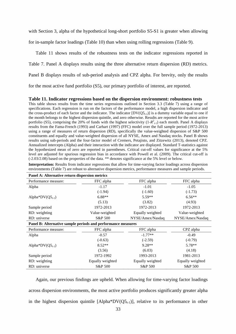
33
with Section 3, alpha of the hypothetical long-short portfolio S5-S1 is greater when allowing
for in-sample factor loadings (Table 10) than when using rolling regressions (Table 9).
Table 11 shows results of the robustness tests on the indicator regressions reported in
Table 7. Panel A displays results using the three alternative return dispersion (RD) metrics.
Panel B displays results of sub-period analysis and CPZ alpha. For brevity, only the results
for the most active fund portfolio (S5), our primary portfolio of interest, are reported.
Table 11. Indicator regressions based on the dispersion environment: robustness tests This table shows results from the time series regressions outlined in Section 3.3 (Table 7) using a range of specifications. Each regression is run on the factors of the performance model, a high dispersion indicator and the cross-product of each factor and the indicator. The indicator [DV(Q5t-1)] is a dummy variable equal to one if the month belongs to the highest dispersion quintile, and zero otherwise. Results are reported for the most active portfolio (S5), comprising the 20% of funds with the highest selectivity (1-R2
t-1) each month. Panel A displays results from the Fama-French (1993) and Carhart (1997) (FFC) model over the full sample period (1972-2013) using a range of measures of return dispersion (RD), specifically the value-weighted dispersion of S&P 500 constituents and equally and value-weighted dispersion of all NYSE, Amex and Nasdaq stocks. Panel B shows results using sub-periods and the four-factor model of Cremers, Petajisto, and Zitzewitz (2013), denoted CPZ. Annualized intercepts (Alpha) and their interaction with the indicator are displayed. Standard T-statistics against the hypothesized mean of zero are reported in parentheses. Critical cut-off values for significance at the 5% level are adjusted for spurious regression bias in accordance with Powell et al. (2009). The critical cut-off is (-2.03/2.08) based on the properties of the data. ** denotes significance at the 5% level or below.
Interpretation: Results from indicator regressions that allow for time-varying factor loadings across dispersion environments (Table 7) are robust to alternative dispersion metrics, performance measures and sample periods.
Panel A: Alternative return dispersion metrics
Performance measure: FFC alpha FFC alpha FFC alpha
Alpha -1.17 (-1.94)
-1.01 (-1.60)
-1.05 (-1.73)
Alpha*DV(Q5t-1) 6.88** (5.13)
5.59** (3.82)
6.56** (4.93)
Sample period 1972-2013 1972-2013 1972-2013 RD: weighting Value-weighted Equally weighted Value-weighted RD: universe S&P 500 NYSE/Amex/Nasdaq NYSE/Amex/Nasdaq
Panel B: Alternative sample periods and performance measures
Performance measure: FFC alpha FFC alpha CPZ alpha
Alpha -0.57 (-0.63)
-1.77** (-2.59)
-0.49 (-0.79)
Alpha*DV(Q5t-1) 8.52** (3.56)
9.28** (6.03)
5.78** (4.18)
Sample period 1972-1992 1993-2013 1981-2013 RD: weighting Equally weighted Equally weighted Equally weighted RD: universe S&P 500 S&P 500 S&P 500
Again, our previous findings are upheld. When allowing for time-varying factor loadings
across dispersion environments, the most active portfolio produces significantly greater alpha
in the highest dispersion quintile [Alpha*DV(Q5t-1)], relative to its performance in other
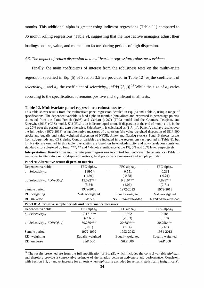
34
months. This additional alpha is greater using indicator regressions (Table 11) compared to
36 month rolling regressions (Table 9), suggesting that the most active managers adjust their
loadings on size, value, and momentum factors during periods of high dispersion.
4.3. The impact of return dispersion in a multivariate regression: robustness evidence
Finally, the main coefficients of interest from the robustness tests on the multivariate
regression specified in Eq. (5) of Section 3.5 are provided in Table 12 [a2, the coefficient of
selectivityi,t-1 and a3, the coefficient of selectivityi,t-1*DV(Q5t-1)].21 While the size of a3 varies
according to the specification, it remains positive and significant in all tests.
Table 12. Multivariate panel regressions: robustness tests This table shows results from the multivariate panel regression detailed in Eq. (5) and Table 8, using a range of specifications. The dependent variable is fund alpha in month t (annualized and expressed in percentage points), estimated from the Fama-French (1993) and Carhart (1997) (FFC) model and the Cremers, Petajisto, and Zitzewitz (2013) (CPZ) model. DV(Q5t-1) is an indicator equal to one if dispersion at the end of month t-1 is in the top 20% over the period, and zero otherwise. Selectivityi,t-1 is calculated as (1-R2
i,t-1). Panel A displays results over the full period (1972-2013) using alternative measures of dispersion (the value-weighted dispersion of S&P 500 stocks and equally and value-weighted dispersion of NYSE, Amex and Nasdaq stocks). Panel B shows results from sub-periods and CPZ alpha. Control variables are included in the regressions (as reported in Table 8), but for brevity are omitted in this table. T-statistics are based on heteroskedasticity and autocorrelation consistent standard errors clustered by fund. ***, ** and * denote significance at the 1%, 5% and 10% level, respectively.
Interpretation: Results from multivariate panel regressions to control for fund-level characteristics (Table 8) are robust to alternative return dispersion metrics, fund performance measures and sample periods.
Panel A: Alternative return dispersion metrics
Dependent variable: FFC alphai,t FFC alphai,t FFC alphai,t
a2: Selectivityi,t-1 -1.995* (-1.91)
-0.551 (-0.58)
-0.231 (-0.21)
a3: Selectivityi,t-1*DV(Q5 t-1) 15.022*** (5.24)
9.810*** (4.06)
7.898*** (2.71)
Sample period 1972-2013 1972-2013 1972-2013 RD: weighting Value-weighted Equally weighted Value-weighted RD: universe S&P 500 NYSE/Amex/Nasdaq NYSE/Amex/Nasdaq
Panel B: Alternative sample periods and performance measures
Dependent variable: FFC alphai,t FFC alphai,t CPZ alphai,t
a2: Selectivityi,t-1 -7.171*** (-2.65)
-1.562 (-1.63)
0.184 (0.19)
a3: Selectivityi,t-1*DV(Q5 t-1) 30.289*** (3.01)
20.689*** (7.14)
20.258*** (7.61)
Sample period 1972-1992 1993-2013 1981-2013
RD: weighting Equally weighted Equally weighted Equally weighted
RD: universe S&P 500 S&P 500 S&P 500
21 The results presented are from the full specification of Eq. (5), which includes the control variable alphai,t-1, and therefore provide a conservative estimate of the relation between activeness and performance. Consistent with Section 3.5, a2 and a3 increase for all tests when alphai,t-1 is excluded (a2 remains statistically insignificant).

35
4.4. Alternative measure of fund activeness: Active Share
In this section, we consider an alternative measure of fund activeness, specifically the
Active Share measure of Cremers and Petajisto (2009). The choice of selectivity (1-R2), as
opposed to Active Share, as the primary measure of active management is derived from the
relative advantages and disadvantages of the two measures in the context of this study. As
noted by Amihud and Goyenko (2013), while Active Share can be measured at any time from
a fund’s holdings with no need for a return history, it only accounts for a fund’s deviation
from a single benchmark index. As R2 can be calculated with respect to multiple benchmarks,
it is better able to detect funds that appear active but are merely passive with respect to
multiple benchmark factors. By estimating alpha from the FFC and CPZ four-factor models
in differing dispersion environments, our aim is to examine whether active funds exploit
sources of return dispersion in addition to the size, value and momentum factors contained in
these models. Calculation of a fund’s R2 with respect to these models enables the
identification of the most active funds as those that also deviate from their additional factors,
making R2 the more intuitive measure of activeness in this case.
However, to examine whether our results are sensitive to the choice of the fund activeness
measure we repeat the tests conducted in Section 3, replacing selectivity with Active Share.
Data for Active Share are obtained from Antti Petajisto’s website for the period 1980 to 2009
and calculated manually from 2010 to 2013.22 As we examine both FFC and CPZ alphas, the
sample period used in this sub-section spans January 1981 to December 2013, to enable
consistent comparison. As with our treatment of R2, we trim the top and bottom 0.5% of
funds each month according to Active Share. This process results in a sample of 1,893 funds
with data on Active Share, with 157,728 fund-month observations.
22 Active Share data are available for 1980 to 2009 from http://www.petajisto.net/data.html (item activeshare_min). As Active Share is calculated quarterly, we take a fund’s monthly Active Share as its Active Share in the quarter to which the month belongs. For the calculation of Active Share from 2009, we obtain index constituent data for the Russell indexes from Russell and for the remaining indices from Thomson Reuters Datastream. These data are combined with fund holdings from Thomson Reuters CDA/Spectrum and stock returns from CRSP.
36
Table 13 displays the key variables of interest for the rolling (Panel A), in-sample (Panel
B) and indicator (Panel C) regressions outlined in Section 3.23 Results are shown for three
performance measures: benchmark-adjusted FFC alpha, traditional FFC alpha and CPZ alpha.
Cremers and Petsjisto (2009) report their results using a benchmark-adjusted specification of
the FFC model, in which fund return in excess of its allocated benchmark index, as opposed
to the risk-free rate, is regressed on the FFC factors. This adjustment to the traditional FFC
model is motivated by the authors’ finding that the benchmark indexes of funds with high
Active Share have significantly negative FFC alphas, reducing the traditional FFC alpha
estimates of the most active funds. Consistent with Cremers and Petajisto (2009), Panels A
and B of Table 13 show that, over our entire sample period, the portfolio of funds with the
highest Active Share scores significantly outperforms that with the lowest scores using
benchmark-adjusted FFC alpha, but not traditional FFC alpha.24
Interestingly, despite the most active funds failing to produce significantly greater
traditional FFC alpha over the entire period, they still outperform the least active funds in the
top dispersion quintile. For example, using rolling regressions, the traditional FFC alpha of the
hypothetical long-short portfolio A5-A1 is 3.75% (T = 2.21), suggesting that any downward
bias is not sufficient to remove all traditional FFC alpha to A5-A1 during times of elevated
dispersion. This further emphasizes the essential role played by high dispersion environments
in the outperformance of the most active funds. More generally, consistent with our results
when activeness is defined by selectivity, the outperformance of the highest, over the lowest,
Active Share funds is greatest in the top dispersion quintile, during which the estimated alpha
to A5-A1 exceeds 3% p.a. in all specifications.
23 Active Share is computed quarterly and the high dispersion indicator is monthly, distorting the interaction between the variables. As such, the multivariate regression cannot be performed for the Active Share measure. 24 Cremers and Petajisto (2009) report a higher benchmark-adjusted FFC alpha to portfolio A5-A1 over the full period: using equivalent in-sample regressions, the authors report alpha to A5-A1 of 2.98% p.a., as opposed to our estimate of 1.14% p.a. This difference stems from the sample period chosen: Cremers and Petajisto (2009) estimate alphas over 1990 to 2003, as opposed to our sample period of 1981 to 2013. When we restrict our tests to 1990 to 2003, we get results for the full period similar to theirs.
37
When weighing up results produced by the Active Share and selectivity measures, the
best comparison can be made using the CPZ model, as the non-zero FFC alphas of Active
Share allocated fund benchmarks may bias results from the traditional FFC model against
Active Share. Further, unlike Active Share, in which the process of calculation results in an
allocated benchmark index, measuring activeness by selectivity does not provide a natural
benchmark with which to adjust the FFC model. The CPZ factors are themselves constructed
using replicable market indexes, therefore mitigating the need to use benchmark-adjusted
returns to control for non-zero alphas in the Active Share benchmarks.
In all tests, results from the CPZ model are qualitatively consistent using Active Share and
selectivity. Regardless of the activeness measure employed, it is during times of elevated
dispersion that the most active fund portfolio produces significantly positive CPZ alpha, and
shows the greatest outperformance relative to the least active funds. The size of the alpha
produced by the most active portfolio in times of high dispersion, however, is smaller when
activeness is measured using Active Share as opposed to selectivity. To illustrate, when using
in-sample regressions to control for factor loadings specific to the dispersion environment, the
highest selectivity portfolio produces CPZ alpha during the top dispersion quintile of 5.26%
p.a. (T = 2.86) (Table 10, Panel D), whereas the highest Active Share portfolio produces CPZ
alpha of 4.53% p.a. (T = 2.58) (Table 13, Panel B). The lower alphas using Active Share
might be expected given the focus of our research: we aim to identify funds which can
capitalize on sources of high return dispersion in addition to the size, value and momentum
factors of the FFC and CPZ models. Classification of highly active funds using selectivity
filters out managers who increase their return merely through increasing loadings on these
easily identifiable sources of dispersion. Classification using Active Share, in contrast, focuses
on a fund’s deviation from a single benchmark index, and hence will less easily detect
managers whose active bets extend beyond the size, value and momentum factors combined.

38
Table 13. Active Share: robustness tests This table displays results from multiple tests where activeness is measured using Active Share (Cremers and Petajisto, 2009). Average annualized four-factor alpha to active funds is shown over the period 1981 to 2013 (396 months). Alpha is estimated from the benchmark-adjusted Fama-French (1993) and Carhart (1997) (FFC) model, the traditional FFC model and the Cremers, Petajisto, and Zitzewitz (2013) (CPZ) model. Active Share portfolios are formed by sorting funds each month t into quintiles, resulting in five portfolios of differing activeness A1 to A5, where A1 (A5) makes up the 20% of funds with the lowest (highest) Active Share scores. Panel A shows alphas obtained through rolling regressions as outlined in Section 3.1 (Table 4). For each portfolio, results are presented for the highest dispersion quintile (Q5), comprising the 20% of months that begin with the highest levels of return dispersion (RDt-1). Panel B shows results from the in-sample regressions outlined in Section 3.3 (Table 6). Panel C shows results from the indicator regressions outlined in Section 3.3 (Table 7). Each regression is run on the FFC or CPZ model factors, a high dispersion indicator, and the cross-product of each factor and the high dispersion indicator. The high dispersion indicator [DV(Q5t-1)] is a dummy variable equal to one if the month belongs to the highest dispersion quintile, and zero otherwise. Annualized intercepts (Alpha) and their interaction with the high dispersion indicator are displayed. In all panels, standard T-statistics are omitted for brevity. In Panels A and B, ***, ** and * denote significance at the 1%, 5% and 10% level, respectively. In Panel C, critical cut-off values for significance at the 5% level are adjusted for spurious regression bias (Powell et al., 2009) to (-2.03/2.08) based on the properties of the data (** denotes significance at the 5% level or below).
Interpretation: Alphas for the most active fund portfolio in times of high dispersion, both relative to the least active funds and the alpha produced in lower dispersion environments, are qualitatively consistent when activeness is measured by Active Share (shown in this table) and selectivity (shown in prior tables).
Panel A: Alpha from rolling regressions
Benchmark-adjusted FFC alpha FFC alpha CPZ alpha
(RDt-1) A5 (high) A5-A1 All (RDt-1) A5 (high) A5-A1 All (RDt-1) A5 (high) A5-A1 All
Q5 (high) 2.41 3.32** 0.13 Q5 (high) 2.18 3.75** 0.01 Q5 (high) 3.28* 4.58*** 0.37
Q5-Q1 3.50** 1.30 Q5-Q1 3.04 1.14 Q5-Q1 2.87 0.82
Q5-Q(1-4) 2.87* 1.23 Q5-Q(1-4) 2.86 0.79 Q5-Q(1-4) 3.20* 0.93
Overall 0.11 1.30** -0.85*** Overall -0.10 0.79 -0.62* Overall 0.71 1.69*** -0.37
Panel B: Alpha from in-sample factor loadings
Benchmark-adjusted FFC alpha FFC alpha CPZ alpha
(RDt-1) A5 (high) A5-A1 All (RDt-1) A5 (high) A5-A1 All (RDt-1) A5 (high) A5-A1 All
Q5 (high) 2.49 3.73** -0.11 Q5 (high) 3.61* 4.54** 0.72 Q5 (high) 4.53*** 5.39*** 0.99
Overall -0.23 1.14* -1.18*** Overall -0.62 0.29 -0.85* Overall 0.70 1.77*** -0.40
Panel C: Alpha from indicator regressions
Benchmark-adjusted FFC alpha FFC alpha CPZ alpha
Fund portfolio: A1 (low) … A5 (high) All Fund portfolio: A1 (low) … A5 (high) All Fund portfolio: A1 (low) … A5 (high) All
Alpha -1.18** -0.48 -1.05** Alpha -0.77** -1.05 -0.85 Alpha -0.95** -0.18 -0.57
Alpha*DV(Q5t-1) -0.06 2.98** 0.95 Alpha*DV(Q5t-1) -0.16 4.71** 1.58 Alpha*DV(Q5t-1) 0.09 4.72** 1.56
39
4.5. Further robustness tests
In additional tests, we measure performance by alpha estimated from the single-factor
Capital Asset Pricing Model (CAPM) and the three-factor model of Fama and French (1993).
We also measure performance by alpha from a five factor model in which the four FFC
factors are augmented with the aggregate liquidity factor of Pastor and Stambaugh (2003), in
order to control for the possibility that the superior performance of the most active managers
in times of high dispersion stems from exposure to market wide liquidity risk.25 Results from
all specifications are consistent with those presented, and are therefore omitted for brevity.
We further examine whether funds which are consistently highly active outperform those
which are less consistently so, during times of high dispersion. If we sort funds into quintile
portfolios according to the number of months each appears in the highest selectivity portfolio
over the sample period, FFC alpha produced during the highest dispersion quintile
monotonically increases with the consistency rank of the portfolio.
4.6. Alternative explanations: recessions and mutual fund performance
There is evidence in the literature suggesting that actively managed funds outperform in
economic downturns, providing insurance against recessions (e.g., Moskowitz, 2000;
Kosowski, 2011; Glode, 2011; Kacperczyk, van Nieuwerburgh, and Veldkamp, 2014a).
Glode (2011) finds that the value of active management lies in providing higher risk-adjusted
returns in recessions, when investors have a higher marginal utility of wealth. Given that
return dispersion has been shown to possess countercyclical properties (e.g., Loungani, Rush,
and Tave, 1990; Gomes, Kogan, and Zhang, 2003; Stivers, 2003; Zhang, 2005), it is possible
that periods of high return dispersion simply coincide with recessionary periods, falsely
attributing increases in performance to the opportunity presented by high dispersion.
25 Pastor and Stambaugh (2003) liquidity data are available from http://finance.wharton.upenn.edu/~stambaugh/.
40
To gauge the relative impact on our results of dispersion and the business cycle, we
conduct the in-sample regression analysis outlined in Section 3.3 and reported in Table 6,
stratifying the sample period according to a number of market conditions.26 Specifically, we
examine FFC alpha to active funds in times of low to medium return dispersion (dispersion
quintiles one to four) and high dispersion (dispersion quintile five), and during economic
expansions and recessions as defined by the NBER.27 We then split the months in the highest
dispersion quintile into expansionary and recessionary months, to examine whether the
outperformance of the most active funds in times of elevated dispersion is concentrated in
periods of economic growth or decline. Finally, we split recessionary months into those also
in the highest dispersion quintile and those in the remaining quintiles, to see whether,
conversely, outperformance in recessions is concentrated in times of high dispersion. The
results are presented in Panel A of Appendix Table A.2.
Over our 1972 to 2013 sample period, of the 101 months in the highest dispersion quintile
[RD(Q5)], 66 (65%) occur during expansions and 35 (35%) are during recessions. Of the 72
recessionary months in the overall sample period, 37 (51%) are in months of low to medium
return dispersion [RD(Q1-4)] and 35 (49%) are in RD(Q5). As can be seen in the table, the
overall fund sample produces negative FFC alpha in months of low to medium return
dispersion and in expansions, and statistically insignificant alpha during times of high return
dispersion and during recessions. However, while the most active fund portfolio produces
positive alpha and significantly outperforms the least active portfolio during the highest
dispersion quintile as a whole, such a result does not exist in recessionary months as a whole
over which no fund portfolio is able to achieve significant alpha.
26 In-sample regression analysis is chosen for methodological consistency with the recession literature (e.g., Moskowitz, 2000; Kosowski, 2011) and because our previous analysis highlights the importance of controlling for in-sample factor loadings specific to the market environment in question. However results are qualitatively consistent if 36 month rolling regressions are used, as described in Section 3.1. 27 The use of NBER business cycle dates is consistent with the aforementioned literature on mutual fund performance over the business cycle.
41
Further stratifying the high dispersion and recessionary periods yields interesting results.
Splitting the months in the top dispersion quintile into those in expansions and recessions has
no qualitative impact on our findings. Irrespective of whether the economy is expanding or
contracting in elevated dispersion months, the highest selectivity portfolio produces
significantly positive FFC alpha and outperforms the lowest selectivity portfolio. The extent
of outperformance of the most over the least active funds is 6.87% p.a. (T = 3.01) in
expansionary periods of elevated dispersion and 5.26% p.a. (T = 1.92) in recessionary periods
of elevated dispersion. However, when recessionary months are divided into those in the top
dispersion quintile and those outside of it, the outperformance of the most active funds in
recessionary periods of high dispersion does not also exist in recessionary periods of lower
dispersion. Thus evidence suggests that, while the state of the business cycle has little impact
on the outperformance of the most active funds in times of high dispersion, the dispersion
environment does affect the ability of highly active funds to outperform in recessions.
The literature on fund performance over the business cycle examines the performance of
funds overall, rather than funds segregated by the activeness of their strategies. To provide a
more general horse race of the impact of recessions and high stock return dispersion on fund
performance, we conduct the multivariate regressions specified in Eq. (5), but remove
selectivity, and the interaction between selectivity and the high dispersion indicator, from the
right hand side of the equation. We use three specifications of the regression: the first
includes the high dispersion indicator, the second replaces the high dispersion indicator with
a recession indicator equal to one if the month is within a recession, and zero otherwise, and
the third includes both the high dispersion and recession indicators in order to test for the
separate effects of elevated dispersion and economic contractions. For greater consistency
with Kacperczyk, van Nieuwerburgh, and Veldkamp (2014a), who examine the impact of
recessions controlling for fund-level characteristics, in this test we calculate FFC alpha using
42
factor loadings from 12 month, as opposed to 36 month, rolling regressions. All control
variables are demeaned. As can be seen in Panel B of Table A.2, the high return dispersion
indicator and the recession indicator are each positive and significant when they are included
alone in the regression, and remain significant when included together in the specification
(column three). When both are included, the coefficient on the high dispersion indicator is of
a similar magnitude to that on the recession indicator. Overall, these results suggest that
periods of elevated dispersion have a positive effect on alpha for the fund sample as a whole,
beyond that coming from recessions. Further, the positive relation between fund activeness
and performance is driven by return dispersion, as opposed to business cycle fluctuations.
5. Investing in funds based on return dispersion and R2
Results thus far suggest that the most active funds are able to react to a high level of
return dispersion by implementing strategies that result in significant alpha, both relative to
the least active funds and to their own performance in times of lower active opportunity. This
provides investors with information to aid in their selection of funds in the cross-section, as
well as time series information to assist in their choice of when to invest in active funds. An
investor who places their money with the most active managers after observing the first
month of top-quintile dispersion, and reduces their investment when dispersion falls out of
the top quintile, would realize significant outperformance over our sample. However such a
strategy could not be implemented in real time, as it is only possible to identify the 20% of
months with the highest dispersion once a period has come to a close. We therefore examine
whether an ex ante strategy derived from our findings could produce significant alpha.
5.1. Active/passive switching strategy based on dispersion and R2
Consider an investor at the end of month t-1, who is facing a choice of whether to invest
in active funds in month t, or whether to invest passively in a fund that tracks a market index.
43
The investor will know the return dispersion realized in month t-1, as well as in all the
months previously. To estimate whether dispersion in month t-1 is relatively high, they can
calculate whether it would be ranked in the top x% of the past y months. Subsequently, they
can follow an active/passive fund switching strategy such that they will invest in active funds
in month t if dispersion in month t-1 is above the defined cut-off, and invest passively
otherwise. As discussed in Section 2.2, such a strategy is facilitated by significant persistence
in the high dispersion environment. Consequently, there is little risk that an investor would
invest in active funds on the observation of high dispersion in month t-1, only for dispersion
to drop substantially in month t.
Table 14 displays the FFC and CPZ alphas from this strategy, where x = 20%, y = 120
months (ten years), return dispersion is calculated as in Eq. (1) and the passive investment
vehicle is the S&P 500 index.28 The S&P 500 was the first index to be tracked by a publicly-
available passive fund, the first such fund being formed in late 1976. As such, we are able to
test the strategy over the period 1977 to 2013. Returns from the strategy each month t are
calculated as the net return to the active fund portfolio in each column of the table if
dispersion in month t-1 is in the top 20% of the past 120 months, and the equally weighted
average net return to passive S&P 500 index funds otherwise.29 We subtract the monthly risk-
free rate to obtain excess returns. These excess returns are then regressed on the factors of the
FFC and CPZ models over the months of our sample.
We examine the results of this switching strategy using seven alternative portfolios during
the months of active investment. The first five columns display alphas from the strategy when
equal weights are placed in those funds that comprise selectivity portfolios S1 to S5 during
28 The choice of y = 120 is driven by observing high dispersion environments roughly every ten years (Fig. 1). The S&P 500 is chosen because it is the most popular choice for passive fund investment. It is also the most cited fund benchmark in our sample and the first index to be tracked by an index fund available to individual investors (the Vanguard Index Trust), and therefore provides the longest time series for our strategy. 29 From 1998 onwards, CRSP directly identifies S&P 500 index funds as those with Lipper Objective Code SP. To identify S&P 500 index funds before 1998, we take those funds classified as SP in 1998, and add any funds whose name indicates their objective as an S&P 500 fund, e.g. those that contain “S&P 500.”
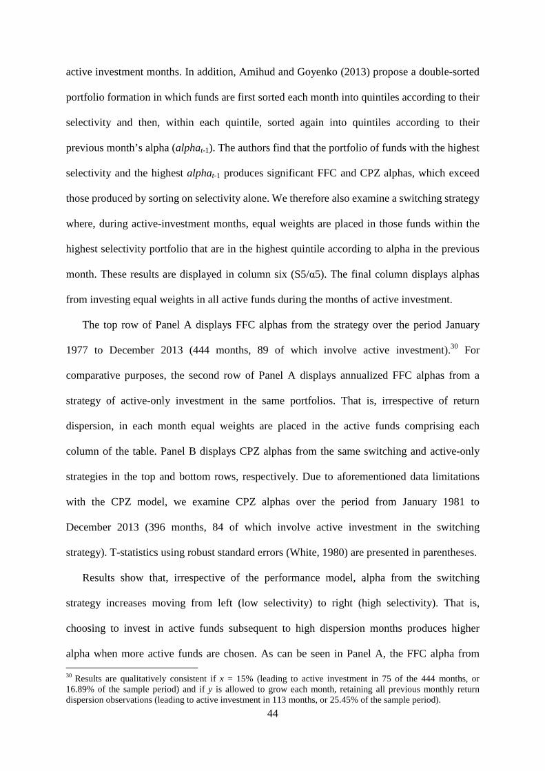
44
active investment months. In addition, Amihud and Goyenko (2013) propose a double-sorted
portfolio formation in which funds are first sorted each month into quintiles according to their
selectivity and then, within each quintile, sorted again into quintiles according to their
previous month’s alpha (alphat-1). The authors find that the portfolio of funds with the highest
selectivity and the highest alphat-1 produces significant FFC and CPZ alphas, which exceed
those produced by sorting on selectivity alone. We therefore also examine a switching strategy
where, during active-investment months, equal weights are placed in those funds within the
highest selectivity portfolio that are in the highest quintile according to alpha in the previous
month. These results are displayed in column six (S5/α5). The final column displays alphas
from investing equal weights in all active funds during the months of active investment.
The top row of Panel A displays FFC alphas from the strategy over the period January
1977 to December 2013 (444 months, 89 of which involve active investment).30 For
comparative purposes, the second row of Panel A displays annualized FFC alphas from a
strategy of active-only investment in the same portfolios. That is, irrespective of return
dispersion, in each month equal weights are placed in the active funds comprising each
column of the table. Panel B displays CPZ alphas from the same switching and active-only
strategies in the top and bottom rows, respectively. Due to aforementioned data limitations
with the CPZ model, we examine CPZ alphas over the period from January 1981 to
December 2013 (396 months, 84 of which involve active investment in the switching
strategy). T-statistics using robust standard errors (White, 1980) are presented in parentheses.
Results show that, irrespective of the performance model, alpha from the switching
strategy increases moving from left (low selectivity) to right (high selectivity). That is,
choosing to invest in active funds subsequent to high dispersion months produces higher
alpha when more active funds are chosen. As can be seen in Panel A, the FFC alpha from 30 Results are qualitatively consistent if x = 15% (leading to active investment in 75 of the 444 months, or 16.89% of the sample period) and if y is allowed to grow each month, retaining all previous monthly return dispersion observations (leading to active investment in 113 months, or 25.45% of the sample period).
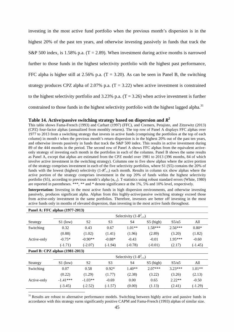
45
investing in the most active fund portfolio when the previous month’s dispersion is in the
highest 20% of the past ten years, and otherwise investing passively in funds that track the
S&P 500 index, is 1.58% p.a. (T = 2.89). When investment during active months is narrowed
further to those funds in the highest selectivity portfolio with the highest past performance,
FFC alpha is higher still at 2.56% p.a. (T = 3.20). As can be seen in Panel B, the switching
strategy produces CPZ alpha of 2.07% p.a. (T = 3.22) when active investment is constrained
to the highest selectivity portfolio and 3.23% p.a. (T = 3.26) when active investment is further
constrained to those funds in the highest selectivity portfolio with the highest lagged alpha.31
Table 14. Active/passive switching strategy based on dispersion and R2 This table shows Fama-French (1993) and Carhart (1997) (FFC), and Cremers, Petajisto, and Zitzewitz (2013) (CPZ) four-factor alphas (annualized from monthly returns). The top row of Panel A displays FFC alphas over 1977 to 2013 from a switching strategy that invests in active funds (comprising the portfolios at the top of each column) in month t when the previous month’s return dispersion is in the highest 20% out of the past ten years, and otherwise invests passively in funds that track the S&P 500 index. This results in active investment during 89 of the 444 months in the period. The second row of Panel A shows FFC alphas from the equivalent active-only strategy of investing each month in the portfolios in each of the columns. Panel B shows the same results as Panel A, except that alphas are estimated from the CPZ model over 1981 to 2013 (396 months, 84 of which involve active investment in the switching strategy). Columns one to five show alphas where the active portion of the strategy comprises investment in each of the five selectivity portfolios, where S1 (S5) contains the 20% of funds with the lowest (highest) selectivity (1-R2
t-1) each month. Results in column six show alphas where the active portion of the strategy comprises investment in the top 20% of funds within the highest selectivity portfolio (S5), according to previous month’s alpha (αt-1). T-statistics using robust standard errors (White, 1980) are reported in parentheses. ***, ** and * denote significance at the 1%, 5% and 10% level, respectively.
Interpretation: Investing in the most active funds in high dispersion environments, and otherwise investing passively, produces significant alpha. Alphas from this highly-active/passive switching strategy exceed those from active-only investment in the same portfolios. Therefore, investors are better off investing in the most active funds only in months of elevated dispersion, than investing in the most active funds throughout.
Panel A: FFC alphas (1977-2013)
Selectivity (1-R2t-1)
Strategy S1 (low) S2 S3 S4 S5 (high) S5/α5 All
Switching 0.32 0.43 0.67 1.01** 1.58*** 2.56*** 0.80*
(0.88) (1.02) (1.41) (1.96) (2.89) (3.20) (1.82)
Active-only -0.75* -0.90** -0.88* -0.43 -0.01 1.95*** -0.60
(-1.71) (-2.07) (-1.94) (-0.78) (-0.01) (2.17) (-1.45)
Panel B: CPZ alphas (1981-2013)
Selectivity (1-R2t-1)
Strategy S1 (low) S2 S3 S4 S5 (high) S5/α5 All
Switching 0.07 0.58 0.92* 1.40** 2.07*** 3.23*** 1.01**
(0.22) (1.29) (1.77) (2.38) (3.22) (3.26) (2.13)
Active-only -1.41*** -1.03** -0.69 0.00 0.65 2.22** -0.50
(-3.45) (-2.52) (-1.57) (0.00) (1.13) (2.41) (-1.29)
31 Results are robust to alternative performance models. Switching between highly active and passive funds in accordance with this strategy earns significantly positive CAPM and Fama-French (1993) alphas of similar size.

46
All results from the switching strategy exceed those from active-only investment in the
same portfolios. In particular, while (consistent with Amihud and Goyenko, 2013) investing
every month in those funds in portfolio S5/α5 produces significant FFC and CPZ alphas of
1.95% p.a. (T = 2.17) and 2.22% p.a. (T = 2.41), respectively, this performance is exceeded
by the switching strategy we propose.32 As such, investors are better off investing in the most
active funds only during periods of high dispersion, and otherwise investing passively, than
investing in the most active funds throughout.
An additional advantage of our active/passive switching strategy is its relative simplicity
to implement. To maintain equal weights in the funds in the lowest R2t-1/highest alphat-1
portfolio, an investor who pursues the double sort-strategy of Amihud and Goyenko (2013)
would need to make frequent changes to the composition of the fund portfolio, including
monthly rebalancing of the weights in each fund. In contrast, our active/passive switching
strategy only requires active investment in approximately 20% of months. To illustrate,
following the switching strategy over our 1977 to 2013 sample period requires active
investment in only 89 of the 444 months. In the remaining 355 months, an investor could
place their wealth in a passive fund that tracks the S&P 500 index, therefore requiring less
frequent changes to fund investment.
5.2. An additional consideration: fund loads
The analysis in the preceding section does not include a potentially important cost. While
the alpha presented is calculated net of all management expenses and 12-b fees for both
active and passive funds, thus far no consideration has been given to fund loads.
To remove the potential impact of fund loads, we restrict our analysis to no-load funds in
the highly active (S5 and S5/α5) and passive fund portfolios. This largely eliminates the costs
32 Amihud and Goyenko (2013) examine the period from 1990 to 2010. While the annual alphas from active-only investment in portfolios S5 and S5/α5 are higher over the 1990 to 2010 period, we find they are still exceeded by the active/passive switching strategy conducted on the same portfolios by over 60 basis points.
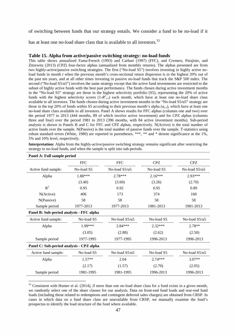
47
of switching between funds that our strategy entails. We consider a fund to be no-load if it
has at least one no-load share class that is available to all investors.33
Table 15. Alpha from active/passive switching strategy: no-load funds This table shows annualized Fama-French (1993) and Carhart (1997) (FFC), and Cremers, Petajisto, and Zitzewitz (2013) (CPZ) four-factor alphas (annualized from monthly returns). The alphas presented are from two highly-active/passive switching strategies. The first (“No-load S5”) involves investing in highly active no-load funds in month t when the previous month’s cross-sectional return dispersion is in the highest 20% out of the past ten years, and at all other times investing in passive no-load funds that track the S&P 500 index. The second (“No-load S5/α5”) involves the same strategy except that the active fund investments are restricted to the subset of highly active funds with the best past performance. The funds chosen during active investment months in the “No-load S5” strategy are those in the highest selectivity portfolio (S5), representing the 20% of active funds with the highest selectivity scores (1-R2
t-1) each month, which have at least one no-load share class available to all investors. The funds chosen during active investment months in the “No-load S5/α5” strategy are those in the top 20% of funds within S5 according to their previous month’s alpha (αt-1), which have at least one no-load share class available to all investors. Panel A shows results for FFC alphas (columns one and two) over the period 1977 to 2013 (444 months, 89 of which involve active investment) and for CPZ alphas (columns three and four) over the period 1981 to 2013 (396 months, with 84 active investment months). Sub-period analysis is shown in Panels B and C for FFC and CPZ alphas, respectively. N(Active) is the total number of active funds over the sample. N(Passive) is the total number of passive funds over the sample. T-statistics using robust standard errors (White, 1980) are reported in parentheses. ***, ** and * denote significance at the 1%, 5% and 10% level, respectively.
Interpretation: Alpha from the highly-active/passive switching strategy remains significant after restricting the strategy to no-load funds, and when the sample is split into sub-periods.
Panel A: Full sample period
FFC FFC CPZ CPZ
Active fund sample: No-load S5 No-load S5/α5 No-load S5 No-load S5/α5
Alpha 1.88*** 2.78*** 2.16*** 2.93***
(3.40) (3.60) (3.26) (2.70)
R2 0.95 0.92 0.95 0.89
N(Active) 406 173 374 160
N(Passive) 58 58 58 58
Sample period 1977-2013 1977-2013 1981-2013 1981-2013
Panel B: Sub-period analysis - FFC alpha
Active fund sample: No-load S5 No-load S5/α5 No-load S5 No-load S5/α5
Alpha 1.99*** 2.84*** 2.32*** 2.78**
(3.05) (2.88) (2.62) (2.50)
Sample period 1977-1995 1977-1995 1996-2013 1996-2013
Panel C: Sub-period analysis - CPZ alpha
Active fund sample: No-load S5 No-load S5/α5 No-load S5 No-load S5/α5
Alpha 1.57** 2.04 2.74*** 3.07**
(2.17) (1.57) (2.70) (2.05)
Sample period 1981-1995 1981-1995 1996-2013 1996-2013
33 Consistent with Hunter et al. (2014), if more than one no-load share class for a fund exists in a given month, we randomly select one of the share classes for our analysis. Data on front-end fund loads and rear-end fund loads (including those related to redemptions and contingent deferred sales charges) are obtained from CRSP. In cases in which data on a fund share class are unavailable from CRSP, we manually examine the fund’s prospectus to identify the load structure of the fund where available.
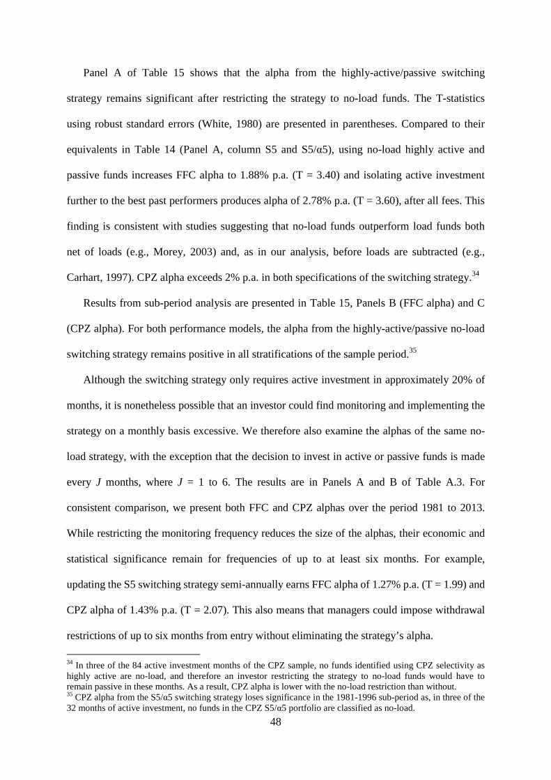
48
Panel A of Table 15 shows that the alpha from the highly-active/passive switching
strategy remains significant after restricting the strategy to no-load funds. The T-statistics
using robust standard errors (White, 1980) are presented in parentheses. Compared to their
equivalents in Table 14 (Panel A, column S5 and S5/α5), using no-load highly active and
passive funds increases FFC alpha to 1.88% p.a. (T = 3.40) and isolating active investment
further to the best past performers produces alpha of 2.78% p.a. (T = 3.60), after all fees. This
finding is consistent with studies suggesting that no-load funds outperform load funds both
net of loads (e.g., Morey, 2003) and, as in our analysis, before loads are subtracted (e.g.,
Carhart, 1997). CPZ alpha exceeds 2% p.a. in both specifications of the switching strategy.34
Results from sub-period analysis are presented in Table 15, Panels B (FFC alpha) and C
(CPZ alpha). For both performance models, the alpha from the highly-active/passive no-load
switching strategy remains positive in all stratifications of the sample period.35
Although the switching strategy only requires active investment in approximately 20% of
months, it is nonetheless possible that an investor could find monitoring and implementing the
strategy on a monthly basis excessive. We therefore also examine the alphas of the same no-
load strategy, with the exception that the decision to invest in active or passive funds is made
every J months, where J = 1 to 6. The results are in Panels A and B of Table A.3. For
consistent comparison, we present both FFC and CPZ alphas over the period 1981 to 2013.
While restricting the monitoring frequency reduces the size of the alphas, their economic and
statistical significance remain for frequencies of up to at least six months. For example,
updating the S5 switching strategy semi-annually earns FFC alpha of 1.27% p.a. (T = 1.99) and
CPZ alpha of 1.43% p.a. (T = 2.07). This also means that managers could impose withdrawal
restrictions of up to six months from entry without eliminating the strategy’s alpha.
34 In three of the 84 active investment months of the CPZ sample, no funds identified using CPZ selectivity as highly active are no-load, and therefore an investor restricting the strategy to no-load funds would have to remain passive in these months. As a result, CPZ alpha is lower with the no-load restriction than without. 35 CPZ alpha from the S5/α5 switching strategy loses significance in the 1981-1996 sub-period as, in three of the 32 months of active investment, no funds in the CPZ S5/α5 portfolio are classified as no-load.
49
In further tests (Table A.3, Panels C and D), we find that results are robust to imposing an
additional one-month gap between the calculation of return dispersion and implementation of
the strategy. To illustrate, an altered S5/α5 switching strategy, in which the dispersion
observed in month t is used to determine whether to invest in active or passive funds in
month t+2 (as opposed to month t+1), earns FFC alpha of 1.73% p.a. (T = 1.93) and CPZ
alpha of 1.95% p.a. (T = 1.77). As such, the strategy would remain profitable in the presence
of an additional one month information delay about the level of return dispersion in the
market.36
Our findings suggest that knowledge of the dispersion environment provides valuable
information to investors regarding the active/passive fund choice. No matter how skilled the
fund manager, the pursuit of active strategies can only produce performance that differs
discernibly from the market when returns of stocks are sufficiently dispersed. When cross-
sectional return dispersion is low, so is the impact of active strategies, and yet the higher fees
charged by active mutual fund managers remain. Choosing only to invest in the most active
funds on the observation of high return dispersion in the market, and investing passively
when return dispersion is low, produces significantly positive alpha over our sample period.
6. Conclusion
Despite the large and growing active funds industry, empirical evidence suggests that the
average active fund produces negative risk-adjusted performance after expenses. This is
commonly taken as evidence that active managers do not add sufficient value, and thus lack
the necessary skills, to justify the fees they charge. Existing studies generally look at
performance over an entire sample period, without conditioning on the active opportunity set.
Yet active opportunity is not constant. Active managers aim to outperform by undertaking
36 Waiting to implement the strategy until month t+3 results in insignificant alpha (Table A.3, Panels C and D). However given the speed of data availability, not least the Russell-Parametric Cross-Sectional Volatility Indexes that are released up to date at monthly frequencies, this finding does not impair the feasibility of the strategy.
50
active bets that tilt their portfolios towards better performing stocks, while avoiding the worst
performers in the market. Even for the most highly skilled of managers, this cannot
successfully lead to outperformance unless the returns of stocks are sufficiently dispersed. As
a result, periods of low cross-sectional dispersion in stock returns could mask the existence of
managerial skill.
In this study we show that those managers who pursue the most active strategies produce
significant outperformance in times of high cross-sectional dispersion in returns. During
times of high dispersion, a portfolio of the most active funds significantly outperforms a
portfolio of the least active funds. This is in contrast to lower dispersion months, during
which the difference in performance between the most and least active funds is not generally
significant. In addition, only the most active fund portfolio consistently produces
performance in months of high dispersion that exceeds its performance in other months.
An investor’s choice of when to invest in active funds can be as important to generating
outperformance as the choice of which funds to invest in. An active/passive switching
strategy of investing in the most active funds when the prior month’s return dispersion is
ranked in the top 20% of the past ten years, and otherwise investing passively in S&P 500
index funds, produces significant alpha after all fees of over 1.8% p.a. irrespective of the
performance model. When active investment is isolated further to the funds in the most active
portfolio with the best past performance, alpha from the switching strategy increases to over
2.7% p.a. after fees. In all specifications, alpha produced from this active/passive switching
strategy is considerably greater than the alpha achieved by investing in active funds
throughout. Altogether, our findings suggest that consideration of the return dispersion
environment can provide important insights for ex ante decisions regarding active investment,
as well as for the ex post evaluation of active funds.
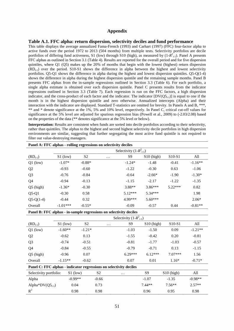
51
Appendix
Table A.1. FFC alpha: return dispersion, selectivity deciles and fund performance This table displays the average annualized Fama-French (1993) and Carhart (1997) (FFC) four-factor alpha to active funds over the period 1972 to 2013 (504 months) from multiple tests. Selectivity portfolios are decile portfolios of differing fund activeness, S1 (low) through S10 (high), as measured by (1-R2
t-1). Panel A presents FFC alphas as outlined in Section 3.1 (Table 4). Results are reported for the overall period and for five dispersion quintiles, where Q1 (Q5) makes up the 20% of months that begin with the lowest (highest) return dispersion (RDt-1) over the period. S10-S1 shows the difference in alpha between the highest and lowest selectivity portfolios. Q5-Q1 shows the difference in alpha during the highest and lowest dispersion quintiles. Q5-Q(1-4) shows the difference in alpha during the highest dispersion quintile and the remaining sample months. Panel B presents FFC alphas from the in-sample regressions outlined in Section 3.3 (Table 6). For each portfolio, a single alpha estimate is obtained over each dispersion quintile. Panel C presents results from the indicator regressions outlined in Section 3.3 (Table 7). Each regression is run on the FFC factors, a high dispersion indicator, and the cross-product of each factor and the indicator. The indicator [DV(Q5t-1)] is equal to one if the month is in the highest dispersion quintile and zero otherwise. Annualized intercepts (Alpha) and their interaction with the indicator are displayed. Standard T-statistics are omitted for brevity. In Panels A and B, ***, ** and * denote significance at the 1%, 5% and 10% level, respectively. In Panel C, critical cut-off values for significance at the 5% level are adjusted for spurious regression bias (Powell et al., 2009) to (-2.03/2.08) based on the properties of the data (** denotes significance at the 5% level or below).
Interpretation: Results are consistent when funds are sorted into decile portfolios according to their selectivity, rather than quintiles. The alphas to the highest and second highest selectivity decile portfolios in high dispersion environments are similar, suggesting that further segregating the most active fund quintile is not required to filter out value-destroying managers.
Panel A: FFC alphas - rolling regressions on selectivity deciles
Selectivity (1-R2t-1)
(RDt-1) S1 (low) S2 … S9 S10 (high) S10-S1 All
Q1 (low) -1.07* -0.88* -1.24* -1.48 -0.41 -1.16**
Q2 -0.93 -0.60 -1.22 -0.30 0.63 -1.06
Q3 -0.76 -0.84 -0.64 -2.66* -1.90 -1.30*
Q4 -0.94 -0.13 -1.15 -2.17 -1.22 -1.35
Q5 (high) -1.36* -0.30 3.88** 3.86*** 5.22*** 0.82
Q5-Q1 -0.30 0.58 5.12*** 5.34*** 1.98
Q5-Q(1-4) -0.44 0.32 4.99*** 5.60*** 2.06*
Overall -1.01*** -0.55* -0.09 -0.57 0.44 -0.81**
Panel B: FFC alphas - in-sample regressions on selectivity deciles
Selectivity (1-R2t-1)
(RDt-1) S1 (low) S2 … S9 S10 (high) S10-S1 All
Q1 (low) -1.60** -1.21* -1.03 -1.50 0.09 -1.21**
Q2 -0.62 0.13 -1.55 -0.42 0.20 -0.81
Q3 -0.74 -0.51 -0.81 -1.77 -1.03 -0.57
Q4 -0.84 -0.55 -0.79 -0.71 0.13 -1.15
Q5 (high) -0.96 0.07 6.29*** 6.12*** 7.07*** 1.56
Overall -1.15** -0.62 0.07 0.01 1.16* -0.71*
Panel C: FFC alphas - indicator regressions on selectivity deciles
Selectivity portfolio: S1 (low) S2 … S9 S10 (high) All
Alpha -0.99** -0.66 -1.07 -1.35 -0.98**
Alpha*DV(Q5t-1) 0.04 0.73 7.44** 7.56** 2.57**
R2 0.98 0.98 0.96 0.95 0.98
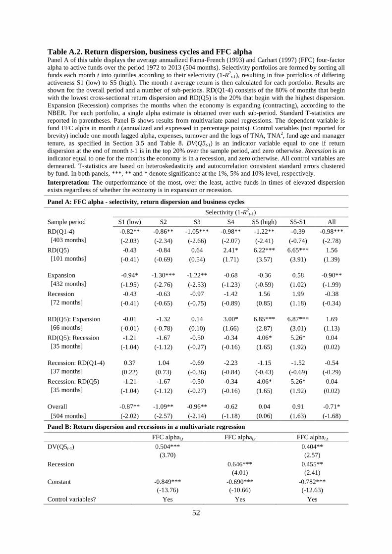
52
Table A.2. Return dispersion, business cycles and FFC alpha Panel A of this table displays the average annualized Fama-French (1993) and Carhart (1997) (FFC) four-factor alpha to active funds over the period 1972 to 2013 (504 months). Selectivity portfolios are formed by sorting all funds each month t into quintiles according to their selectivity (1-R2
t-1), resulting in five portfolios of differing activeness S1 (low) to S5 (high). The month t average return is then calculated for each portfolio. Results are shown for the overall period and a number of sub-periods. RD(Q1-4) consists of the 80% of months that begin with the lowest cross-sectional return dispersion and RD(Q5) is the 20% that begin with the highest dispersion. Expansion (Recession) comprises the months when the economy is expanding (contracting), according to the NBER. For each portfolio, a single alpha estimate is obtained over each sub-period. Standard T-statistics are reported in parentheses. Panel B shows results from multivariate panel regressions. The dependent variable is fund FFC alpha in month t (annualized and expressed in percentage points). Control variables (not reported for brevity) include one month lagged alpha, expenses, turnover and the logs of TNA, TNA2, fund age and manager tenure, as specified in Section 3.5 and Table 8. DV(Q5t-1) is an indicator variable equal to one if return dispersion at the end of month t-1 is in the top 20% over the sample period, and zero otherwise. Recession is an indicator equal to one for the months the economy is in a recession, and zero otherwise. All control variables are demeaned. T-statistics are based on heteroskedasticity and autocorrelation consistent standard errors clustered by fund. In both panels, ***, ** and * denote significance at the 1%, 5% and 10% level, respectively. Interpretation: The outperformance of the most, over the least, active funds in times of elevated dispersion exists regardless of whether the economy is in expansion or recession.
Panel A: FFC alpha - selectivity, return dispersion and business cycles
Selectivity (1-R2t-1)
Sample period S1 (low) S2 S3 S4 S5 (high) S5-S1 All
RD(Q1-4) -0.82** -0.86** -1.05*** -0.98** -1.22** -0.39 -0.98*** [403 months] (-2.03) (-2.34) (-2.66) (-2.07) (-2.41) (-0.74) (-2.78)
RD(Q5) -0.43 -0.84 0.64 2.41* 6.22*** 6.65*** 1.56 [101 months] (-0.41) (-0.69) (0.54) (1.71) (3.57) (3.91) (1.39)
Expansion -0.94* -1.30*** -1.22** -0.68 -0.36 0.58 -0.90** [432 months] (-1.95) (-2.76) (-2.53) (-1.23) (-0.59) (1.02) (-1.99)
Recession -0.43 -0.63 -0.97 -1.42 1.56 1.99 -0.38 [72 months] (-0.41) (-0.65) (-0.75) (-0.89) (0.85) (1.18) (-0.34)
RD(Q5): Expansion -0.01 -1.32 0.14 3.00* 6.85*** 6.87*** 1.69 [66 months] (-0.01) (-0.78) (0.10) (1.66) (2.87) (3.01) (1.13)
RD(Q5): Recession -1.21 -1.67 -0.50 -0.34 4.06* 5.26* 0.04 [35 months] (-1.04) (-1.12) (-0.27) (-0.16) (1.65) (1.92) (0.02)
Recession: RD(Q1-4) 0.37 1.04 -0.69 -2.23 -1.15 -1.52 -0.54 [37 months] (0.22) (0.73) (-0.36) (-0.84) (-0.43) (-0.69) (-0.29)
Recession: RD(Q5) -1.21 -1.67 -0.50 -0.34 4.06* 5.26* 0.04 [35 months] (-1.04) (-1.12) (-0.27) (-0.16) (1.65) (1.92) (0.02)
Overall -0.87** -1.09** -0.96** -0.62 0.04 0.91 -0.71*
[504 months] (-2.02) (-2.57) (-2.14) (-1.18) (0.06) (1.63) (-1.68)
Panel B: Return dispersion and recessions in a multivariate regression
FFC alphai,t FFC alphai,t FFC alphai,t
DV(Q5t-1) 0.504*** (3.70)
0.404** (2.57)
Recession
0.646*** (4.01)
0.455** (2.41)
Constant -0.849*** (-13.76)
-0.690*** (-10.66)
-0.782*** (-12.63)
Control variables? Yes Yes Yes

53
Table A.3. Alpha from switching strategy: withdrawal and implementation delays This table shows annualized Fama-French (1993) and Carhart (1997) (FFC), and Cremers, Petajisto, and Zitzewitz (2013) (CPZ) four-factor alphas (annualized from monthly returns) from a range of modifications to the switching strategies outlined in Table 15. Panels A and B show alphas from the same highly active/passive switching strategies as described in Table 15, except that the decision to invest in active or passive funds based on the prior month’s return dispersion is made every J months, where J = 1 to 6 (J = 1 is the baseline strategy outlined in the description of Table 15). Panels C and D show alphas from the same highly active/passive switching strategies as described in Table 15, except that the return dispersion in month t is used to decide whether to invest in active or passive funds in month t+K , where K = 1 to 3 (K = 1 is the baseline strategy outlined in the description of Table 15). Unlike Table 15, in this table all alphas are shown for the period from 1981 to 2013, to enable direct comparison. T-statistics using robust standard errors (White, 1980) are reported in parentheses. ***, ** and * denote significance at the 1%, 5% and 10% level, respectively.
Interpretation: Alphas from the highly-active/passive switching strategies remain significant in the face of withdrawal or implementation delays.
Panel A: FFC alphas (1981-2013) - withdrawal delays
Withdrawal delay (J months)
Active portfolio J=1
(baseline) J=2 J=3 J=4 J=5 J=6
No-load S5 2.08*** 1.19* 1.72*** 1.15* 1.56** 1.27**
(3.56) (1.95) (2.88) (1.81) (2.47) (1.99)
No-load S5/α5 3.36*** 2.54*** 2.58*** 1.65* 2.63** 2.14**
(4.08) (2.67) (2.70) (1.78) (2.32) (2.04)
Panel B: CPZ alphas (1981-2013) - withdrawal delays
Withdrawal delay (J months)
Active portfolio J=1
(baseline) J=2 J=3 J=4 J=5 J=6
No-load S5 2.16*** 1.30** 1.84*** 1.34* 1.76** 1.43**
(3.26) (2.01) (2.80) (1.90) (2.52) (2.07)
No-load S5/α5 2.93*** 2.98** 2.96** 1.94* 3.19** 1.88
(2.70) (2.57) (2.47) (1.82) (2.46) (1.55)
Panel C: FFC alphas (1981-2013) - implementation delays
Panel D: CPZ alphas (1981-2013) - implementation delays
Implementation delay (K months) Implementation delay (K months)
Active portfolio K=1
(baseline) K=2 K=3 Active portfolio
K=1
(baseline) K=2 K=3
No-load S5 2.08*** 1.13* 0.70 No-load S5 2.16*** 1.16* 0.85
(3.56) (1.86) (1.07) (3.26) (1.80) (1.21)
No-load S5/α5 3.36*** 1.73* 0.74 No-load S5/α5 2.93*** 1.95* 1.32
(4.08) (1.93) (0.71) (2.70) (1.77) (1.15)
54
References
Amihud, Y., Goyenko, R., 2013. Mutual fund’s R2 as predictor of performance. Review of
Financial Studies 26, 667-694.
Ankrim, E., Ding, Z., 2002. Cross-sectional volatility and return dispersion. Financial
Analysts Journal 58, 67-73.
Bekaert, G., Harvey, C., 1997. Emerging equity market volatility. Journal of Financial
Economics 43, 29-77.
Baker, M., Litov, L., Wachter, J., Wurgler, J., 2010. Can mutual fund managers pick stocks?
Evidence from their trades prior to earnings announcements. Journal of Financial and
Quantitative Analysis 45, 1111-1131.
Bessembinder, H., Chan, K., Seguin, P., 1996. An empirical examination of information,
differences of opinion, and trading activity. Journal of Financial Economics 40, 105-134.
Bouchey, P., Fjelstad, M., Vadlamudi, H., 2011. Measuring alpha potential in the market. The
Journal of Index Investing 2, 40-47.
Brands, S., Brown, S., Gallagher, D., 2005. Portfolio concentration and investment manager
performance. International Review of Finance 5, 149-174.
Brainard, S., Cutler, D., 1993. Sectorial shifts and cyclical unemployment reconsidered. The
Quarterly Journal of Economics 108, 219-243.
Carhart, M., 1997. On persistence in mutual fund performance. Journal of Finance 52, 57-82.
Chen, H., Desai, H., Krishnamurthy, S., 2013. A first look at mutual funds that use short
sales. Journal of Financial and Quantitative Analysis 48, 761-787.
Connolly, R., Stivers, C., 2006. Information content and other characteristics of the daily
cross-sectional dispersion in stock returns. Journal of Empirical Finance 13, 79-112.
Cremers, M., Ferreira, M., Matos, P., Starks, L., 2015. Indexing and active fund management:
international evidence. Journal of Financial Economics, Forthcoming.
Cremers, M., Petajisto, A., 2009. How active is your fund manager? A new measure that
predicts performance. Review of Financial Studies 22, 3329-3365.
55
Cremers, M., Petajisto, A., Zitzewitz, E., 2013. Should benchmark indices have alpha?
Revisiting performance evaluation. Critical Finance Review 2, 1-48.
Da, Z., Gao, P., Jagannathan, R., 2011. Impatient trading, liquidity provision, and stock
selection by mutual funds. Review of Financial Studies 24, 675-720.
Daniel, K., Grinblatt, M., Titman, S., Wermers, R., 1997. Measuring mutual fund
performance with characteristic-based benchmarks. Journal of Finance 52, 1035-1058.
De Silva, H., Sapra, S., Thorley, S., 2001. Return dispersion and active management.
Financial Analysts Journal 57, 29-42.
Del Guercio, D., Reuter, J., 2014. Mutual fund performance and the incentive to generate
alpha. Journal of Finance 69, 1673-1704.
Dong, X., Feng, S., Sadka, R., 2014. Liquidity risk and mutual fund performance.
Unpublished working paper. Baruch College.
Evans, R., 2010. Mutual fund incubation. Journal of Finance 65, 1581-1611.
Fama, E., French, K., 1993. Common risk factors in the returns on stocks and bonds. Journal
of Financial Economics 33, 3-56.
Glode, V., 2011. Why mutual funds “underperform.” Journal of Financial Economics 99,
546-559.
Gomes, J., Kogan, L., Zhang, L., 2003. Equilibrium cross section of returns. Journal of
Political Economy 111, 693-732.
Gorman, L., Sapra, S., Weigand, R., 2010. The cross-sectional dispersion of stock returns,
alpha and the information ratio. Journal of Investing 19, 113-127.
Gruber, M., 1996. Another puzzle: the growth in actively managed mutual funds. Journal of
Finance 51, 783-810.
Gupta-Mukherjee, S., 2013. When active fund managers deviate from their peers:
Implications for fund performance. Journal of Banking and Finance 37, 1286-1305.
Huang, J., Sialm, C., Zhang, H., 2011. Risk shifting and mutual fund performance. Review of
Financial Studies 24, 2575–2616.
56
Huij, J., Derwall, J., 2011. Global equity fund performance, portfolio concentration, and the
fundamental law of active management. Journal of Banking and Finance 35, 155-165.
Hunter, D., Kandel, E., Kandel, S., Wermers, R., 2014. Mutual fund performance evaluation
with active peer benchmarks. Journal of Financial Economics 112, 1-29.
Kacperczyk, M., Seru, A., 2007. Fund manager use of public information: new evidence on
managerial skills. Journal of Finance 62, 485-528.
Kacperczyk, M., Sialm, C., Zheng, L., 2005. On the industry concentration of actively
managed equity mutual funds. Journal of Finance 60, 1983-2011.
Kacperczyk, M., Sialm, C., Zheng, L., 2008. Unobserved actions of mutual funds. Review of
Financial Studies 21, 2379-2416.
Kacperczyk, M., van Nieuwerburgh, S., Veldkamp, L., 2014a. A rational theory of mutual
funds’ attention allocation. Unpublished working paper. Imperial College London.
Kacperczyk, M., van Nieuwerburgh, S., Veldkamp, L., 2014b. Time-varying fund manager
skill. Journal of Finance 69, 1455-1484.
Koijen, R., 2014. The cross-section of managerial ability, incentives, and risk preferences.
Journal of Finance 69, 1051-1098.
Kosowski, R., 2011. Do mutual funds perform when it matters most to investors? US mutual
fund performance and risk in recessions and expansions. Quarterly Journal of Finance 1,
607-664.
Loungani, P., Rush, M., Tave, W., 1990. Stock market dispersion and unemployment. Journal
of Monetary Economics 25, 367-388.
Malkiel, B., 1995. Returns from investing in equity mutual funds 1971 to 1991. Journal of
Finance 50, 549-572.
Morey, M., 2003. Should you carry the load? A comprehensive analysis of load and no-load
mutual fund out-of-sample performance. Journal of Banking and Finance 27, 1245-1271.
Moskowitz, T., 2000. Mutual fund performance: An empirical decomposition into stock-
picking talent, style, transactions costs, and expenses: Discussion. Journal of Finance 55,
1695-1703.
57
Pástor, Ľ., Stambaugh, R., 2002. Investing in equity mutual funds. Journal of Financial
Economics 63, 351-380.
Pástor, Ľ., Stambaugh, R., 2003. Liquidity risk and expected stock returns. Journal of
Political Economy 111, 642-685.
Petajisto, A., 2013. Active share and mutual fund performance. Financial Analysts Journal
69, 73-93.
Powell, J., Shi, J., Smith, T., Whaley, R., 2009. Political regimes, business cycles,
seasonalities, and returns. Journal of Banking and Finance 33, 1112-1128.
Sensoy, B., 2009. Performance evaluation and self-designated benchmark indexes in the
mutual fund industry. Journal of Financial Economics 92, 25-39.
Stivers, C., 2003. Firm-level return dispersion and the future volatility of aggregate stock
market returns. Journal of Financial Markets 6, 389-411.
Stivers, C., Sun, L., 2010. Cross-sectional return dispersion and time variation in value and
momentum premiums. Journal of Financial and Quantitative Analysis 45, 987-1014.
Sun, Z., Wang, A., Zheng, L., 2012. The road less travelled: strategy distinctiveness and
hedge fund performance. Review of Financial Studies 25, 96-143.
Titman, S., and Tiu, C., 2011. Do the best hedge funds hedge? Review of Financial Studies
24, 123-168.
Wermers, R., 2003a. Are mutual fund shareholders compensated for active management
“bets”? Unpublished working paper. University of Maryland.
Wermers, R., 2003b. Is money really “smart”? New evidence on the relation between mutual
fund flows, manager behavior, and performance persistence. Unpublished working
paper. University of Maryland.
White, H., 1980. A heteroskedasticity-consistent covariance matrix estimator and a direct test
for heteroskedasticity. Econometrica 48, 817–838.
Zhang, L., 2005. The value premium. Journal of Finance 60, 67-103.