1

Where is the Warm Glow? Donated Labour in the Health & Social Work Industries1

Alasdair Rutherford2 Department of Economics University of Stirling

The “Warm Glow” theory of worker motivation in nonprofit organisations predicts

that wages will be lower in the voluntary sector than for equivalent workers in the

private and public sectors. Empirical findings, however, are mixed. Focussing on the

Health & Social Work industries, we examine differences in levels of unpaid overtime

between the sectors to test for the existence of a warm-glow effect. Although levels of

unpaid overtime are significantly higher in voluntary sector, we find that this is

insufficient to explain the wage premiums earned in this sector. 3

JEL Codes: J31; J45; L31

Keywords: Unpaid Overtime; Working Hours; Wage differentials; Warm Glow;

Nonprofit Introduction

1 Working Paper (2008). This version: February 2010. This work was supported by the Economic and Social Research Council (ESRC). Please contact the author before citing this work. 2 Alasdair Rutherford, University of Stirling, Cottrell 3X10, Stirling, Scotland FK9 4LA Tel: +44 (0)1786 467 488 Email: ar34 at stir.ac.uk Web: http://acrutherford.blogspot.com 3 The author gratefully acknowledges the helpful comments and suggestions made by David Bell, Sascha Becker and participants at the NCVO “Researching the Voluntary Sector” conference 2008. All errors and omissions remain the sole responsibility of the author.

2

Introduction

In this paper we compare working hours between the private, public and voluntary

sectors. Specifically, we investigate the role of unpaid overtime as “donated labour”.

Traditional warm-glow analysis uses wage differences between the private, public and

voluntary sectors as a measurement of donated labour. This, however, does not

control for differences in effort between the sectors. Here we test for differences in

hours worked between the sectors. Our contribution in this paper is to provide a more

robust exploration of nonprofit wage differentials, as well as adding an additional

explanation to the literature on unpaid overtime.

This paper uses ten years of pooled cross-sectional data from the UK Quarterly

Labour Force Survey (LFS) in order to examine levels of unpaid overtime at a

disaggregated industry level in industries where voluntary sector concentration is

relatively high. The rotating-panel structure of the UK LFS allows us to estimate a

fixed effects model to control for unobserved worker heterogeneity. We focus on the

Health & Social Work industries for two reasons: firstly, to reduce the unobserved

heterogeneity between organisations and jobs by narrowing the activities undertaken;

secondly, to examine the caring industries where theory predicts that warm glow

should be strongest.

We begin by examining whether there are significant levels of donated labour

observed in the voluntary sector, expressed as hours of unpaid overtime. Next, we

test whether donated labour explains the voluntary sector wage premium found in the

caring industries. Evidence is found of donated labour through significantly higher

levels of unpaid overtime for voluntary sector workers at all industry detail levels.

Wage equations are estimated with wages adjusted for these additional hours of

unpaid work, showing that for female workers there is a significant warm-glow wage

discount even after controlling for unobserved worker heterogeneity.

Empirical Literature on Sector Differentials and Donated Labour

There is an extensive literature on the apparent wage premium earned by workers in

the public sectors (see Bender (1998) for a review). The stylised facts from this

3

literature are that there is a public sector premium, it is greatest for women and

minorities, but it has generally been decreasing over time. Disney & Gosling (1998)

used the General Household Survey (GHS) and British Household Panel Survey

(BHPS) to estimate the public sector premium in the UK after taking worker

characteristics into account. They found that for men the premium fell from 5% in

1983 to only 1% by the mid-1990’s. However, for women the public sector premium

increased over the same period from 11% to 14%.

Relatively little empirical work has been done where the voluntary sector is examined

separately as a third sector. There has been some past research attempting to estimate

nonprofit or voluntary sector wage differences as a measure of warm glow, primarily

using US data. Weisbrod (1983) examined wage differences between lawyers

employed by nonprofit and for-profit firms, and found evidence of a nonprofit wage

discount of ~20%. His analysis of a job choice equation suggested that lawyers in the

nonprofit sector held different preferences to those employed in the private sector.

Preston (1989) conducted an analysis of the nonprofit sector wage differential for

white-collar workers using Current Population Survey (CPS) in the US, and found a

significant nonprofit sector discount of 18% even after controlling for differences in

human capital and other worker and job characteristics. She found a larger

differential for male workers than female workers. It is suggested that a selectivity

bias might be present, and this is tested for using a two-stage sector choice model, and

also analysing a limited sector switching model. She concludes that a “donative

labour” hypothesis is supported by the findings, but that the presence of unobserved

heterogeneity in worker characteristics that might affect their productivity has not

been completely ruled out.

Leete (2001) used US census data for 1990 and found little evidence of a difference

between the private and voluntary sectors overall. However, she did find some

significant differences at the disaggregated industry level. Although the industry

categories used in Leete’s paper differ from those in the UK LFS, it is possible to

identify some that are relevant to the industry classifications examined in this paper.

4

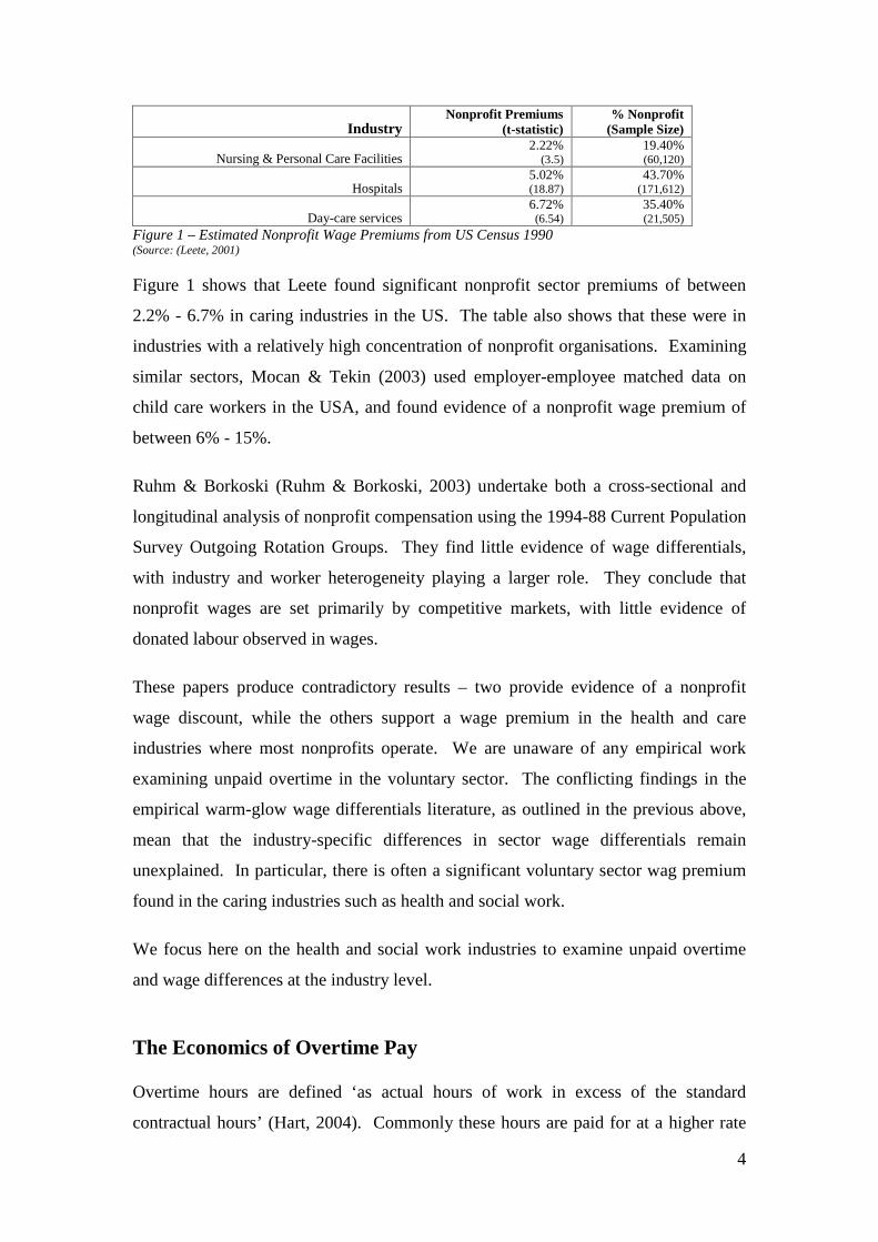
Industry Nonprofit Premiums

(t-statistic) % Nonprofit

(Sample Size)

Nursing & Personal Care Facilities 2.22%

(3.5) 19.40% (60,120)

Hospitals 5.02% (18.87)

43.70% (171,612)

Day-care services 6.72% (6.54)

35.40% (21,505)

Figure 1 – Estimated Nonprofit Wage Premiums from US Census 1990 (Source: (Leete, 2001)

Figure 1 shows that Leete found significant nonprofit sector premiums of between

2.2% - 6.7% in caring industries in the US. The table also shows that these were in

industries with a relatively high concentration of nonprofit organisations. Examining

similar sectors, Mocan & Tekin (2003) used employer-employee matched data on

child care workers in the USA, and found evidence of a nonprofit wage premium of

between 6% - 15%.

Ruhm & Borkoski (Ruhm & Borkoski, 2003) undertake both a cross-sectional and

longitudinal analysis of nonprofit compensation using the 1994-88 Current Population

Survey Outgoing Rotation Groups. They find little evidence of wage differentials,

with industry and worker heterogeneity playing a larger role. They conclude that

nonprofit wages are set primarily by competitive markets, with little evidence of

donated labour observed in wages.

These papers produce contradictory results – two provide evidence of a nonprofit

wage discount, while the others support a wage premium in the health and care

industries where most nonprofits operate. We are unaware of any empirical work

examining unpaid overtime in the voluntary sector. The conflicting findings in the

empirical warm-glow wage differentials literature, as outlined in the previous above,

mean that the industry-specific differences in sector wage differentials remain

unexplained. In particular, there is often a significant voluntary sector wag premium

found in the caring industries such as health and social work.

We focus here on the health and social work industries to examine unpaid overtime

and wage differences at the industry level.

The Economics of Overtime Pay

Overtime hours are defined ‘as actual hours of work in excess of the standard

contractual hours’ (Hart, 2004). Commonly these hours are paid for at a higher rate

5

than basic working hours. However, a more recent literature has begun to explore the

phenomenon of reported unpaid overtime. Workers may work either paid or unpaid

overtime in addition to their contracted hours, or they may work a combination of

both, or neither.

The total weekly hours Hi for a worker i are therefore shown below, where hb are the

usual contracted hours, hpo are the hours of paid overtime and huo are the hours of

unpaid overtime.

�� � �� � ��� � �� (1)

The total weekly pay Wi received by a worker i is shown below, where wb is the basic

hourly wage rate, and π is the overtime premium.

� � ���� � ����� (2)

The overtime literature suggests that the term ‘unpaid overtime’ is a misnomer.

Although there is no explicit contractual payment for hours of unpaid overtime

worked, the question that the literature address is: how is the worker compensated for

these hours?

Bell & Hart (2003) use the 1998 British New Earnings survey to investigate the

relationship between basic hourly pay and overtime premiums. They show that there

is a significant negative relationship, with higher overtime premiums being associated

with lower basic hourly wages. They suggest that overtime premiums are driven by

custom and practice within an industry, and are not related to the length of overtime

worked. Firms therefore can use the variable premium to maintain a competitive

effective wage. This supports an implicit contract between firms and workers over

the effective hourly wage that will be paid, for a given mix of basic and overtime

hours.

Bell & Hart (1999) propose five explanations for the existence of unpaid overtime:

• uncertainty over task completion times;

• auctions for task allocation;

• regulate team performance;

6

• gift exchange;

• compensating differentials.

Firstly, unpaid overtime could permit the adjustment of contracts where there is

uncertainty on behalf of both the employer and the worker about the time required to

undertake a task. With some probability, the worker will undertake additional hours

unpaid to fulfil a contract.

Secondly, employers may allocate work tasks on the basis of ‘bids’ from workers as

to task completion times. Workers have an incentive to understate their task

completion time in order to win the contract, and then work additional hours unpaid to

fulfil it, if the payment from contracted hours still outweighs their outside option.

Thirdly, teams of workers may use unpaid overtime as a regulation device to allow

lower productivity workers additional time to complete tasks where the same wage is

paid to all team members. Effectively, the unpaid overtime allows the informal

adjustment of hourly wage within the team.

Fourthly, employers and workers may enter into an implicit contract, where workers

‘gift’ extra effort in return for a higher basic wage. This extra effort could be in the

form of additional hours unpaid, holding work intensity constant. Although the

exchange is not explicitly contracted over, it is enforced through workplace norms.

Lastly, if wage bargains regarding overtime premiums are reached outside the level of

the relationship between employer and worker, there may be welfare improvements

from negotiating a lower, local rate. The could be reached through an implicit

agreement to undertake a mix of paid and unpaid overtime hours.

The fourth explanation has significance in the nonprofit literature, and could be

relevant in the analysis of sector differences. Bell & Hart find evidence of gift

exchange through the association of unpaid overtime with higher wages. They did not

however find evidence of unpaid overtime being used to adjust rigidities in paid

overtimes rates, tested by examining the link between undertaking both paid and

unpaid overtime.

7

Pannenberg (2005) explores the long-term effects of unpaid overtime using data from

the German Socio-Economic Panel. Pannenberg finds evidence of increased real

wage growth for male workers who work unpaid overtime, robust to the estimation of

a fixed-effects model, but little evidence of a similar significant effect for women.

This supports the role of unpaid overtime as an investment, with a positive expected

value, at least for male workers.

We propose an additional explanation for unpaid overtime: if wages are rigid within

industries across sectors, then the effective wages of workers in mission-motivated

organisations are adjusted by working additional hours of unpaid overtime.

The traditional warm-glow model suggests that workers gain utility from both their

wage and the intrinsic motivation of engaging in a mission-motivated activity. The

utility function Ui of a worker has three arguments: the total wages earned (Wi), the

level of intrinsic utility derived from working in a mission-motivated activity (Gi),

and the hours of leisure time (Li).

�� � �����, ���, ������, ��� (3)

This makes the assumption that warm glow utility is related to the level of

participation in the mission-motivated activity, rather than the worker receiving a

‘lump sum’ utility from working in the sector rather than outside it. This is consistent

with Andreoni’s concept of warm glow, where the level of utility gained is a function

of the size of donation to the public good. Warm-glow utility arises from the

workers’ participation in the provision of the public good, rather than solely from the

public good itself.

This suggests two competing explanations for sector differences in unpaid overtime.

Workers who receive a warm glow from their work could engage in unpaid overtime,

which would lower their effective salary, whilst apparently receiving the same

compensation as other workers. Alternatively unpaid overtime can form part of an

implicit bargain between worker and employer, where additional hours of unpaid

overtime are expected and compensation is paid through a higher hourly wage for the

“official” paid hours of work.

8

We investigate sector wage differences to test between these two explanations for

unpaid overtime in the voluntary sector.

Warm Glow Hypothesis: Workers engage in additional hours of unpaid work due to

the intrinsic utility of working in the mission-oriented sector. The compensation for

the hours of unpaid overtime is received in warm-glow utility.

Gift Exchange Hypothesis: Workers in the voluntary sector engage in implicit

contracts, where additional hours of unpaid work ‘gifted’ to employers are rewarded

with higher basic wages. The compensation for the hours of unpaid overtime is

received through the higher level of the basic wage.

It should be noted that we are examining sector differences between sectors within

industries. It is reasonable to think that there could be a level of job satisfaction

arising from working within the caring industries independent of the legal structure of

the employer. We are looking at differences in warm glow given that the workers are

employed in the caring industries.

Bell & Hart suggest a method of controlling for the effect of unpaid overtime on final

compensation, by calculating an adjusted wage which is then used as the explanatory

variable in a wage equation. First, we test for the existence of a sector difference in

unpaid overtime. Second, we test its impact in an adjusted-wage equation on the

warm-glow sector difference.

The Dataset

This paper uses the UK Quarterly Labour Force Survey (UK LFS) between 1998 and

2007 to create a pooled cross-section dataset with a large enough voluntary sector

sample size to permit detailed analysis. The UK LFS is a quarterly rotating panel

survey of 60,000 households per year in the UK, conducted on a random sample and

carried out by the UK Office of National Statistics (ONS). Each household is

followed for one year, with five quarterly observations, collecting a wide range of

data on wages, job characteristics, education, employers and household make-up.

9

Unobserved Heterogeneity

A recurring problem in estimating differences between sectors is accounting for

unobserved heterogeneity. Are observed sector wage differences explained by

differences between organisational form, or sector selection by workers? There are

two main sources of unobserved heterogeneity that could affect our analysis:

• Heterogeneity in jobs;

• Heterogeneity in workers;

• Unobserved heterogeneity in organisations.

We control for unobserved heterogeneity between jobs by restricting the sample to

detailed industry classifications to allow comparison between similar job activities

and roles. In this paper we estimate sector wage equations at the detailed industry

level, coded using the UK Standard Industrial Classification Of Economic Activities

(SIC(92)).4 The industry classification analysed is SIC(92) N 85 Health & Social

Work.

This broad industry classification includes:

• Human health activities: Hospitals, Nursing Homes, Dental practices,

opticians, etc.

• Veterinary activities: Vets and veterinary hospitals

• Social work activities: Social work services with and without accommodation,

as detailed above

This reduction to more detailed job classification comes at a cost of reduced sample

size.

We control for unobserved heterogeneity between workers by estimating a fixed

effects model using two observations on each worker. This allows us to include an

individual specific fixed effect in the regressions.

4 SIC(92) is a hierarchical 5-digit Industry Classifications code that conforms with and corresponds directly to the European Community Classification of Economic Activities (NACE) Version 1 codes

10

Exploring a Three Sector Workforce

Since the mid-1990’s the questions asked in the LFS allow the identification of

organisations which operate in the Voluntary sector, permitting an analysis of a three

sector model.5

Although the voluntary sector as a whole accounts for only around 4% of the UK

workforce, 60% of the sector operates within the industry classification SIC(92) “85

Health & Social Work”. In contrast, 29% of the Public Sector and 5% of the Private

Sector is engaged within this industry classification. Table 1 below shows the

industry sample size by sector and gender. It shows that although the voluntary sector

makes up a significant proportion of the industry, the private and public sectors are

both still major players within each category.

Sector MALE FEMALE

Freq. Percent Freq. Percent

Private 461 0.150 3057 0.246 Public 2203 0.716 8028 0.646

Voluntary 413 0.134 1351 0.109

TOTAL 3077 12436

Table 1: Sample by Sector and SIC(92) (Source: UK Quarterly Labour Force Survey 1998 – 2007)

Mean values of a selection of key individual and job characteristics are shown in

Table 2 below.

5 See Appendix One for more detail on sector classifications in the UK LFS

11

SAMPLE MEANS

MALE FEMALE Private Public Voluntary ALL Private Public Voluntary ALL

Age (years) 41.23 41.75 43.35 41.88 40.13 41.69 42.20 41.36 Tenure (years) 4.81 10.10 5.14 8.66 5.05 9.85 5.14 8.15 Part-time (%) 0.08 0.04 0.16 0.06 0.38 0.38 0.41 0.38

Temp. Job (%) 0.02 0.07 0.10 0.07 0.02 0.04 0.08 0.04

Unpaid Overtime (hours) 2.81 3.65 5.00 3.71 1.55 2.40 3.68 2.33 Paid Overtime (hours) 5.37 4.45 1.63 4.21 3.83 2.96 1.97 3.07

Total Overtime (hours) 8.18 8.10 6.63 7.91 5.38 5.36 5.65 5.40 Total Work Hours (hours) 45.29 46.14 41.10 45.34 36.22 36.38 35.27 36.22

Hourly Wage (£) 8.96 13.22 11.13 12.30 7.08 10.33 9.15 9.40

Table 2: Sample Means by Sector and gender (Source: UK Quarterly Labour Force Survey 1998 – 2007)

Wave 1 Private Public Voluntary

Wave 5 Freq. Percent Freq. Percent Freq. Percent Private Male 285 0.10 60 0.02 67 0.02

Female 2,262 0.20 187 0.02 209 0.02 Public Male 77 0.03 2,042 0.71 20 0.01

Female 346 0.03 7,447 0.64 82 0.01 Voluntary Male 28 0.01 31 0.01 265 0.09

Female 84 0.01 78 0.01 900 0.08

TOTAL Male 2,875 OBSERVATIONS Female 11,595

Table 3: Sample by Sector in Wave 1 and Wave 5 (Source: UK Quarterly Labour Force Survey 1998 – 2002)

12

In order to control for unobserved worker heterogeneity we also estimate a panel model using

two observations on each worker, one year apart. Due to data constraints we estimate this

model using a smaller sample based on worker observations between 1997 and 2002.

Table 3 above shows the panel sample by sector in wave 1 and wave 5. Workers observed for

at least one wave in the voluntary sector make up 14% (411 observations) of the male sample

and 12% (1,353 observations) of the female sample.

Overtime Data

In the UK LFS respondents are asked about their working hours and overtime. Respondents

are asked to estimate the number of weekly hours of paid and unpaid overtime that they

undertake in their main job.

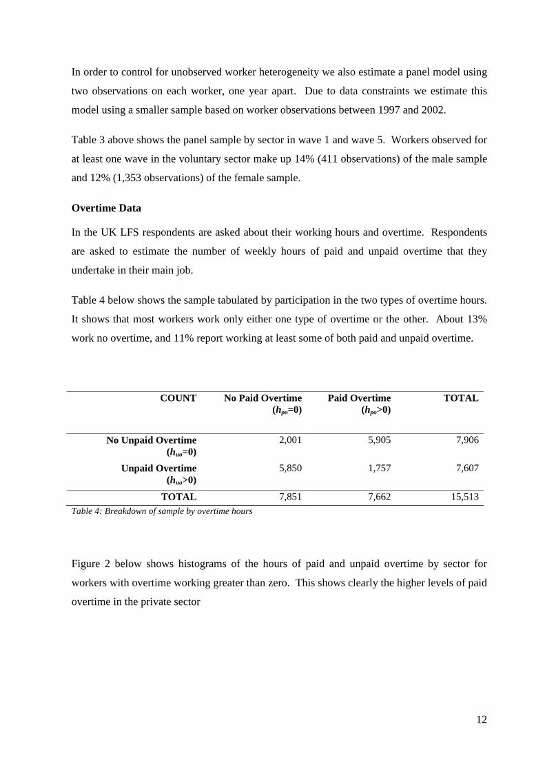
Table 4 below shows the sample tabulated by participation in the two types of overtime hours.

It shows that most workers work only either one type of overtime or the other. About 13%

work no overtime, and 11% report working at least some of both paid and unpaid overtime.

COUNT No Paid Overtime (hpo=0)

Paid Overtime (hpo>0)

TOTAL

No Unpaid Overtime (huo=0)

2,001 5,905 7,906

Unpaid Overtime (huo>0)

5,850 1,757 7,607

TOTAL 7,851 7,662 15,513 Table 4: Breakdown of sample by overtime hours

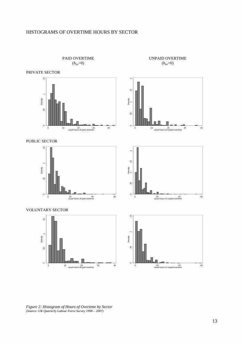
Figure 2 below shows histograms of the hours of paid and unpaid overtime by sector for

workers with overtime working greater than zero. This shows clearly the higher levels of paid

overtime in the private sector

13

HISTOGRAMS OF OVERTIME HOURS BY SECTOR

PAID OVERTIME (hpo>0)

UNPAID OVERTIME (huo>0)

PRIVATE SECTOR

PUBLIC SECTOR

VOLUNTARY SECTOR

Figure 2: Histogram of Hours of Overtime by Sector (Source: UK Quarterly Labour Force Survey 1998 – 2007)

0.0

5.1

.15

Den

sity

0 10 20 30 40usual hours of paid overtime

0.0

5.1

.15

.2D

ensi

ty0 10 20 30 40

usual hours of unpaid overtime

0.0

5.1

.15

Den

sity

0 20 40 60usual hours of paid overtime

0.0

5.1

.15

.2D

ensi

ty

0 20 40 60usual hours of unpaid overtime

0.0

5.1

.15

Den

sity

0 10 20 30 40usual hours of paid overtime

0.0

5.1

.15

Den

sity

0 20 40 60usual hours of unpaid overtime

14

Estimating Working Hours Equations

In order to investigate this, working hours equations (Bell & Hart, 1999) were

estimated to attempt to explain the observed unpaid overtime. Data on unpaid

overtime, paid overtime, total overtime and total working hours were used to estimate

sector differences, conditioning on a range of explanatory variables.

The overtime data contains many observations censored at zero, as it is not possible to

observe negative overtime. Many workers in the sample worked only one type of

overtime, or no overtime at all. In order to control for this, overtime working is

modelled with an underlying propensity to undertake overtime, hi. The overtime

hours are observed when hi is greater than zero, but zero overtime is observed when hi

is less than zero. This is estimated with a Tobit model:

�� �� � 0 � ������ � �� � � !"#�$� � �%&'()�� � �*+� � ,� (4)

�� �� - 0 � ������ � 0

Where:

PUB Sector Dummy for Public Sector workers

VOL Sector Dummy for Voluntary Sector

Xi Education variables (level of highest qualification held);

Characteristics of jobs e.g. organisation size, FT/PT,

permanent/temporary, length of tenure; Characteristics of the workers

e.g. age, experience; Time Dummies for year and quarter

Following Bell & Hart, a proxy for income is included in the estimation of the hours

equations. In order to avoid the endogeneity problem of the joint determination of

wages and hours, w* is the predicted hourly wage from a basic Mincer wage equation,

rather than the observed hourly wage.

ln0���1 � �� � �23� � �� (5)

ln ���4� � ln ��5�

�� � �� � �23� (6)

The coefficients on the sector dummies for the public and voluntary sector relative to

the private sector are shown below in Table 5. Columns one to four show the hours

15

equations for unpaid overtime, paid overtime, total overtime and total hours

respectively.

These estimates suggest that male workers work slightly more unpaid overtime in the

voluntary sector than the private by about 2 hours per week. We find that female

workers work an extra 2.7 hours of weekly unpaid overtime in the voluntary sector.

Levels of paid overtime are also significantly lower in the voluntary sector for both

male and female workers. Male workers in the voluntary sector work significantly

fewer total hours of overtime and total weekly hours of work than those in the private

sector. For female workers there is no significant difference in total overtime, and

evidence of only slightly shorter total weekly hours in the voluntary than the private

sectors.

Although this indicates that there are higher levels of unpaid overtime in the voluntary

sector, controlling for individual and organisational characteristics, it does not control

for unobserved worker heterogeneity. In order to address this we estimate hours

equations on a panel, with two observations on each worker. We estimate two

different specifications: a fixed effects OLS regression, and a random effects Tobit

regression.

Model (a): Fixed Effects

������6 � �� � � !"#�$ � �%&'()� � �*+ � ,�6 (7)

Model (b): Random Effects Tobit

�� ������6 � 0 � ������6 � �� � � !"#�$ � �%&'()� � �*+ � ,�6 (8)

�� ������6 - 0 � ������6 � 0; ��~9�0, :;�

Model (a) is the simplest specification, but it does not account for the censoring of the

hours variable at zero. Model (b) adds this Tobit structure, but at the cost of imposing

a random effects structure to the individual effects. The significant number of zeroes

in the working hours data means that Model (b) is preferred, but both models have

been reported for comparison. Differences in the estimates from the two models are

found mainly in magnitude and statistical significance, but not in the sign of the

estimated effect.

16

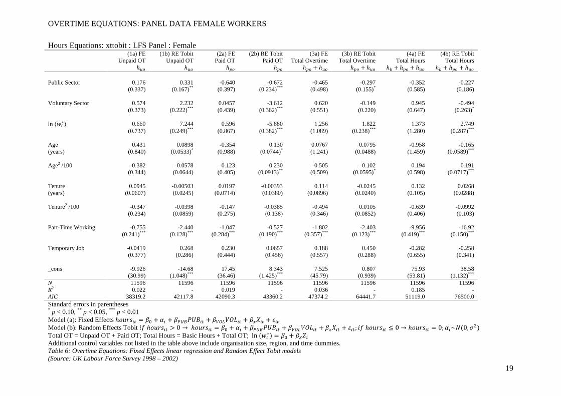
The panel data sample results are shown in Table 6 and Table 7 below. Columns 1(a)

to 4(a) show the fixed effects hours equations for unpaid overtime, paid overtime,

total overtime and total hours respectively. Columns 1(b) to 4(b) show the random

effects tobit hours equations for unpaid overtime, paid overtime, total overtime and

total hours respectively.

Both the fixed effects and the Tobit models find that female voluntary sector workers

work more hours of unpaid overtime, although only the Tobit is significant. The

Tobit estimate of over two hours per week is in-line with the cross-section estimates.

The Tobit model also finds significantly lower levels of paid overtime in the voluntary

sector, with no significant difference in total overtime and only a small difference in

total working hours.

The results for male voluntary sector workers are broadly similar, but with bigger

estimated differences between the private and voluntary sectors. Male voluntary

sector workers also work a significant two hours fewer per week than those in the

private sector. This is also in line with the estimates from the cross-sectional model.

These results appear to support a donated labour theory – workers in the voluntary

sector are providing additional hours of work unpaid, compared to those in the private

sector. This is the case even after controlling for unobserved worker heterogeneity.

To what extent can this be seen as evidence of a “warm glow”?

The literature on unpaid overtime offers an alternative explanation. Workers can use

additional hours of unpaid work to adjust rigid wage contracts. Workers need only

care about the number of hours they work, and the total that they get paid, and not

about exactly how this is recorded. A contract with a low wage and fixed hours could

be equivalent to a contract with a higher wage, but where additional hours unpaid are

an implicit part of the contract. As voluntary sector workers in the HSW industries

are paid a premium, this could in part be explained by the additional hours worked

unpaid. Is there still a sector difference after accounting for these additional hours?

This can be tested by calculating an “Adjusted” hourly wage for each worker based on

the wage per actual hour worked. Calculating this wage for each worker and then

using it as the dependent variable in the wage equations will provide a test for the

17

presence of a “warm glow” through additional unpaid hours a drop in the estimated

sector premium if these hours are unrewarded through basic pay.

18

OVERTIME EQUATIONS: CROSS-SECTIONAL DATA

MALE FEMALE (1) (2) (3) (4) (1) (2) (3) (4)

Unpaid ��

Paid ���

Total OT �� � ��� � ��

Total Hours �� � ��� � ��

Unpaid ��

Paid ���

Total OT �� � ��� � ��

Total Hours �� � ��� � ��

model Public Sector -1.217 -0.809 -1.602 -2.097 0.397 -0.793 -0.475 -1.219 (0.557)** (0.612) (0.438)*** (0.480)*** (0.165)** (0.215)*** (0.148)*** (0.173)*** Voluntary Sector 2.302 -6.887 -2.466 -3.853 2.770 -3.280 0.213 -0.976 (0.658)*** (0.840)*** (0.548)*** (0.600)*** (0.216)*** (0.321)*** (0.206) (0.241)***

ln ���4� 17.58 -12.30 3.627 4.733 9.553 -7.368 1.555 3.683

(0.738)*** (0.838)*** (0.560)*** (0.614)*** (0.271)*** (0.370)*** (0.245)*** (0.287)*** Age 0.214 1.200 0.475 1.439 -0.131 1.270 0.483 0.754 (years) (0.255) (0.298)*** (0.201)** (0.220)*** (0.105) (0.149)*** (0.0967)*** (0.113)*** Age2 /100 -69.67 -100.6 -49.25 -152.9 5.880 -165.0 -58.73 -106.0 (28.99)** (35.62)*** (23.26)** (25.44)*** (12.56) (18.65)*** (11.73)*** (13.75)*** Tenure -0.333 0.239 -0.0556 -0.0234 -0.0890 -0.0148 -0.0755 -0.0547 (years) (0.0651)*** (0.0811)*** (0.0542) (0.0594) (0.0234)*** (0.0333) (0.0222)*** (0.0260)** Tenure2 /100 0.691 -0.491 0.0722 -0.00552 0.137 0.213 0.240 0.219 (0.202)*** (0.262)* (0.171) (0.187) (0.0765)* (0.112)* (0.0741)*** (0.0869)** Part-Time Working -1.536 -1.422 -2.035 -19.44 -2.640 -0.837 -2.838 -17.24 (0.818)* (0.907) (0.627)*** (0.682)*** (0.139)*** (0.190)*** (0.128)*** (0.150)*** Temp. Job 1.264 2.714 2.843 4.579 0.833 -0.519 0.613 0.581 (0.702)* (0.873)*** (0.603)*** (0.662)*** (0.302)*** (0.467) (0.298)** (0.350)* _cons -41.34 8.861 -6.524 13.88 -18.05 -2.986 -4.942 24.80 (4.432)*** (4.866)* (3.354)* (3.667)*** (1.655)*** (2.239) (1.480)*** (1.733)*** sigma _cons 8.227 9.943 7.681 8.513 5.672 8.098 6.008 7.157 (0.158)*** (0.195)*** (0.105)*** (0.109)*** (0.0555)*** (0.0807)*** (0.0421)*** (0.0454)*** N 3077 3077 3077 3077 12436 12436 12436 12436 AIC 12610.4 13485.5 19939.0 21986.5 45230.2 50781.9 72311.0 84318.6 Standard errors in parentheses * p < 0.10, ** p < 0.05, *** p < 0.01 Models 1-4: Tobit �� �� � 0 � ������ � �� � � !"#�$� � �%&'()�� � �*+� � ,�; �� �� - 0 � ������ � 0 Total OT = Unpaid OT + Paid OT; Total Hours = Basic Hours + Total OT; ln ���

4� � �� � �23� Additional control variables not listed in the table above include experience, marital status, number of children, organization size, region and year and quarter dummies. Table 5: Overtime Equation Estimation Results (Source: UK Labour Force Survey 1998 – 2007)

19

OVERTIME EQUATIONS: PANEL DATA FEMALE WORKERS

Hours Equations: xttobit : LFS Panel : Female (1a) FE (1b) RE Tobit (2a) FE (2b) RE Tobit (3a) FE (3b) RE Tobit (4a) FE (4b) RE Tobit Unpaid OT

�� Unpaid OT

�� Paid OT

��� Paid OT

��� Total Overtime

��� � �� Total Overtime

��� � �� Total Hours

�� � ��� � �� Total Hours

�� � ��� � �� Public Sector 0.176 0.331 -0.640 -0.672 -0.465 -0.297 -0.352 -0.227 (0.337) (0.167)** (0.397) (0.234)*** (0.498) (0.155)* (0.585) (0.186) Voluntary Sector 0.574 2.232 0.0457 -3.612 0.620 -0.149 0.945 -0.494 (0.373) (0.222)*** (0.439) (0.362)*** (0.551) (0.220) (0.647) (0.263)* ln ���

4� 0.660 7.244 0.596 -5.880 1.256 1.822 1.373 2.749 (0.737) (0.249)*** (0.867) (0.382)*** (1.089) (0.238)*** (1.280) (0.287)*** Age 0.431 0.0898 -0.354 0.130 0.0767 0.0795 -0.958 -0.165 (years) (0.840) (0.0533)* (0.988) (0.0744)* (1.241) (0.0488) (1.459) (0.0589)*** Age2 /100 -0.382 -0.0578 -0.123 -0.230 -0.505 -0.102 -0.194 0.191 (0.344) (0.0644) (0.405) (0.0913)** (0.509) (0.0595)* (0.598) (0.0717)*** Tenure 0.0945 -0.00503 0.0197 -0.00393 0.114 -0.0245 0.132 0.0268 (years) (0.0607) (0.0245) (0.0714) (0.0380) (0.0896) (0.0240) (0.105) (0.0288) Tenure2 /100 -0.347 -0.0398 -0.147 -0.0385 -0.494 0.0105 -0.639 -0.0992 (0.234) (0.0859) (0.275) (0.138) (0.346) (0.0852) (0.406) (0.103) Part-Time Working -0.755 -2.440 -1.047 -0.527 -1.802 -2.403 -9.956 -16.92 (0.241)*** (0.128)*** (0.284)*** (0.190)*** (0.357)*** (0.123)*** (0.419)*** (0.150)*** Temporary Job -0.0419 0.268 0.230 0.0657 0.188 0.450 -0.282 -0.258 (0.377) (0.286) (0.444) (0.456) (0.557) (0.288) (0.655) (0.341) _cons -9.926 -14.68 17.45 8.343 7.525 0.807 75.93 38.58 (30.99) (1.048)*** (36.46) (1.425)*** (45.79) (0.939) (53.81) (1.132)*** N 11596 11596 11596 11596 11596 11596 11596 11596 R2 0.022 - 0.019 - 0.036 - 0.185 - AIC 38319.2 42117.8 42090.3 43360.2 47374.2 64441.7 51119.0 76500.0 Standard errors in parentheses * p < 0.10, ** p < 0.05, *** p < 0.01 Model (a): Fixed Effects ������6 � �� � <� � � !"#�$�6 � �%&'()��6 � �*+�6 � ,�6 Model (b): Random Effects Tobit �� ������6 � 0 � ������6 � �� � <� � � !"#�$�6 � �%&'()��6 � �*+�6 � ,�6; �� ������6 - 0 � ������6 � 0; <�~9�0, :;� Total OT = Unpaid OT + Paid OT; Total Hours = Basic Hours + Total OT; ln ���

4� � �� � �23� Additional control variables not listed in the table above include organisation size, region, and time dummies. Table 6: Overtime Equations: Fixed Effects linear regression and Random Effect Tobit models (Source: UK Labour Force Survey 1998 – 2002)

20

OVERTIME EQUATIONS: PANEL DATA MALE WORKERS

(1a) FE (1b) RE Tobit (2a) FE (2b) RE Tobit (3a) FE (3b) RE Tobit (4a) FE (4b) RE Tobit Unpaid OT

�� Unpaid OT

�� Paid OT

��� Paid OT

��� Total Overtime

��� � �� Total Overtime

��� � �� Total Hours

�� � ��� � �� Total Hours

�� � ��� � �� Public Sector 0.642 -0.560 -1.249 1.596 -0.607 0.269 -1.321 -0.392 (0.814) (0.583) (1.093) (0.761)** (1.279) (0.506) (1.302) (0.527) Voluntary Sector 0.301 2.919 -0.883 -5.997 -0.582 -0.843 -1.056 -2.376 (0.863) (0.701)*** (1.158) (1.069)*** (1.356) (0.644) (1.381) (0.667)*** ln ���

4� 1.770 13.52 0.755 -9.256 2.525 5.168 3.284 6.510 (1.494) (0.685)*** (2.005) (0.944)*** (2.348) (0.586)*** (2.391) (0.624)*** Age -1.520 0.240 0.630 0.136 -0.889 -0.0391 0.173 0.0314 (years) (1.939) (0.172) (2.602) (0.206) (3.047) (0.137) (3.102) (0.145) Age2 /100 -0.211 -0.237 0.703 -0.326 0.492 -0.0378 0.628 -0.136 (0.799) (0.197) (1.072) (0.241) (1.255) (0.159) (1.278) (0.168) Tenure -0.0129 -0.172 0.0769 -0.135 0.0640 -0.165 -0.120 -0.138 (years) (0.160) (0.0739)** (0.215) (0.101) (0.252) (0.0652)** (0.256) (0.0692)** Tenure2 /100 0.0743 0.334 -0.481 0.607 -0.407 0.424 -0.0476 0.316 (0.507) (0.242) (0.680) (0.336)* (0.797) (0.215)** (0.811) (0.228) Part-Time -1.942 -1.876 -0.962 -2.122 -2.904 -2.222 -9.636 -17.86 (1.082)* (0.798)** (1.452) (0.999)** (1.700)* (0.658)*** (1.731)*** (0.685)*** Temporary Job -0.202 0.845 1.999 3.683 1.798 3.028 2.664 4.582 (0.754) (0.698) (1.012)** (0.970)*** (1.185) (0.647)*** (1.206)** (0.667)*** _cons 66.38 -31.31 -35.05 16.89 31.33 -1.164 23.61 33.28 (73.15) (3.518)*** (98.18) (4.035)*** (114.9) (2.705) (117.0) (2.864)*** N 2875 2875 2875 2875 2875 2875 2875 2875 R2 0.054 - 0.024 - 0.030 - 0.077 - AIC 11002.8 12108.1 12695.0 11801.1 13601.6 18302.1 13705.3 20046.6 Standard errors in parentheses * p < 0.10, ** p < 0.05, *** p < 0.01 Model (a): Fixed Effects ������6 � �� � <� � � !"#�$�6 � �%&'()��6 � �*+�6 � ,�6 Model (b): Random Effects Tobit �� ������6 � 0 � ������6 � �� � <� � � !"#�$�6 � �%&'()��6 � �*+�6 � ,�6; �� ������6 - 0 � ������6 � 0; <�~9�0, :;� Total OT = Unpaid OT + Paid OT; Total Hours = Basic Hours + Total OT; ln ���

4� � �� � �23� Additional control variables not listed in the table above include organisation size, region, and time dummies. Table 7: Overtime Equations: Fixed Effects linear regression and Random Effect Tobit models (Source: UK Labour Force Survey 1998 – 2002)

21

Estimating the Wage Equations

In Figure 3 below the mean hourly wages can be seen by sector over the sample

period.

In all three industries the public sector wages are the highest, followed by the

voluntary sector, and with wages lowest in the private sector. There appears to be a

significant gap between the private sector wages and the other two sectors, while the

public and voluntary sector wages seem broadly similar.

Although this does not take account of differences in individuals’ characteristics, such

as age, education and experience, this suggests that there could be a voluntary sector

premium paid to workers in this sector when compared to the private sector.

We also test the robustness of the findings after controlling for unobserved worker

heterogeneity by estimating a model using the limited panel structure of the LFS.

This allows us to control for potential bias arising from worker selection between

sectors.

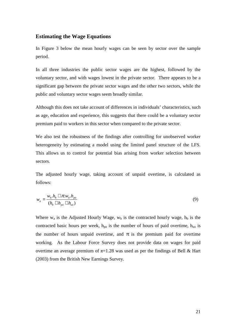
The adjusted hourly wage, taking account of unpaid overtime, is calculated as

follows:

(9)

Where wa is the Adjusted Hourly Wage, wh is the contracted hourly wage, hb is the

contracted basic hours per week, hpo is the number of hours of paid overtime, huo is

the number of hours unpaid overtime, and π is the premium paid for overtime

working. As the Labour Force Survey does not provide data on wages for paid

overtime an average premium of π=1.28 was used as per the findings of Bell & Hart

(2003) from the British New Earnings Survey.

)(

...

uopob

pohbha hhh

hwhww

+++

=π

22

MEAN WAGES 1998 TO 2007 BY SECTOR

Figure 3 - Average Gross Hourly Pay by Sector & Industry between 1998 – 2007 (Source: UK Quarterly Labour Force Survey 1998 – 2007)

23

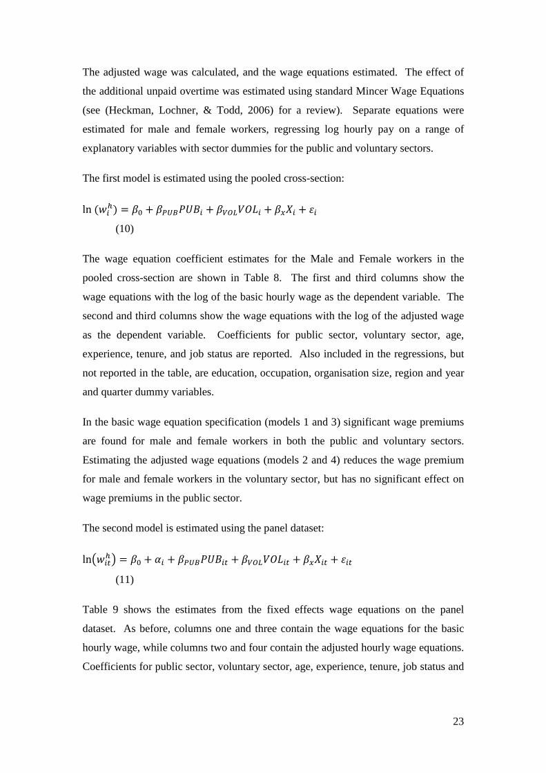
The adjusted wage was calculated, and the wage equations estimated. The effect of

the additional unpaid overtime was estimated using standard Mincer Wage Equations

(see (Heckman, Lochner, & Todd, 2006) for a review). Separate equations were

estimated for male and female workers, regressing log hourly pay on a range of

explanatory variables with sector dummies for the public and voluntary sectors.

The first model is estimated using the pooled cross-section:

ln ����� � �� � � !"#�$� � �%&'()�� � �*+� � ,�

(10)

The wage equation coefficient estimates for the Male and Female workers in the

pooled cross-section are shown in Table 8. The first and third columns show the

wage equations with the log of the basic hourly wage as the dependent variable. The

second and third columns show the wage equations with the log of the adjusted wage

as the dependent variable. Coefficients for public sector, voluntary sector, age,

experience, tenure, and job status are reported. Also included in the regressions, but

not reported in the table, are education, occupation, organisation size, region and year

and quarter dummy variables.

In the basic wage equation specification (models 1 and 3) significant wage premiums

are found for male and female workers in both the public and voluntary sectors.

Estimating the adjusted wage equations (models 2 and 4) reduces the wage premium

for male and female workers in the voluntary sector, but has no significant effect on

wage premiums in the public sector.

The second model is estimated using the panel dataset:

ln0��6�1 � �� � <� � � !"#�$�6 � �%&'()��6 � �*+�6 � ,�6

(11)

Table 9 shows the estimates from the fixed effects wage equations on the panel

dataset. As before, columns one and three contain the wage equations for the basic

hourly wage, while columns two and four contain the adjusted hourly wage equations.

Coefficients for public sector, voluntary sector, age, experience, tenure, job status and

24

organisation size are reported. Also included in the regressions, but not reported in

the table, are education, occupation, region and year and quarter dummy variables.

The basic model estimation (columns 1 and 3) with individuals fixed effects removes

the public and voluntary sector wage premiums found in the pooled cross-section,

suggesting that these are due to unobserved worker heterogeneity.

Estimating the adjusted wage model (columns 2 and 4), to control for overtime

working, now leaves the male voluntary sector wage difference unchanged. However,

female workers have significantly lower effective wages in the voluntary sector than

the private sector. No significant differences between effective wages in the private

and public sectors are found for either male or female workers.

25

WAGE EQUATIONS: POOLED CROSS-SECTION

MALE FEMALE (1) (2) (3) (4) Basic Wage Adjusted Wage Basic Wage Adjusted Wage Public Sector 0.139 0.144 0.147 0.140 (0.0193)*** (0.0184)*** (0.00739)*** (0.00720)*** Voluntary Sector 0.0534 0.0121 0.0861 0.0382 (0.0240)** (0.0229) (0.0102)*** (0.00995)*** Age -0.000428 0.00469 0.0187 0.0239 (years) (0.00892) (0.00854) (0.00479)*** (0.00467)*** Age2 /100 3.507 2.608 0.701 -0.269 (1.025)*** (0.981)*** (0.584) (0.569) Experience 0.0109 0.00825 -0.00149 -0.00498 (years) (0.00451)** (0.00431)* (0.00247) (0.00241)** Experience2 /100 -7.131 -6.401 -4.072 -2.959 (0.839)*** (0.803)*** (0.499)*** (0.486)*** Tenure 0.0145 0.0149 0.0160 0.0148 (years) (0.00232)*** (0.00222)*** (0.00106)*** (0.00103)*** Tenure2 /100 -0.0291 -0.0302 -0.0301 -0.0280 (0.00743)*** (0.00711)*** (0.00363)*** (0.00354)*** Part-Time Working -0.0893 -0.0878 -0.0255 -0.00942 (0.0270)*** (0.0259)*** (0.00590)*** (0.00575) Temporary Job -0.0907 -0.0814 -0.00316 -0.0180 (0.0264)*** (0.0253)*** (0.0147) (0.0144) _cons 1.613 1.546 1.231 1.166 (0.155)*** (0.148)*** (0.0760)*** (0.0741)*** N 3077 3077 12436 12436 R2 0.629 0.582 0.615 0.577 AIC 2100.8 1830.8 5474.1 4842.5 Standard errors in parentheses * p < 0.10, ** p < 0.05, *** p < 0.01 Model 1,3: ln ���

�� � �� � � !"#�$� � �%&'()�� � �*+� � ,� Model 2,4: ln ���

=� � �� � � !"#�$� � �%&'()�� � �*+� � ,� (Additional control variables not listed in the table above include Education, Occupation, Organisation Size, Region, and Time Dummies.) Table 8: Estimated Sector Wage Differences

26

WAGE EQUATIONS: FIXED EFFECTS MODEL (1) (2) (3) (4) Male: Basic Male: Adjusted Female: Basic Female: Adjusted

Public Sector 0.00611 -0.0228 0.0185 0.00638 (0.0469) (0.0476) (0.0251) (0.0256) Voluntary Sector -0.0352 -0.0395 -0.0393 -0.0680 (0.0483) (0.0491) (0.0271) (0.0277)** Age 0.0429 0.0530 0.127 0.122 (Years) (0.0397) (0.0404) (0.0220)*** (0.0225)*** Age2 /100 -0.0115 -0.00731 -0.0855 -0.0742 (0.0459) (0.0466) (0.0256)*** (0.0262)*** Tenure 0.0284 0.0241 0.00102 -0.00133 (Years) (0.00914)*** (0.00928)*** (0.00437) (0.00447)

Tenure2 /100 -0.0792 -0.0713 0.000393 0.00621 (0.0290)*** (0.0294)** (0.0174) (0.0177) Part-Time Working 0.0427 0.0741 0.0825 0.0816 (0.0607) (0.0617) (0.0174)*** (0.0178)*** Temporary Job -0.112 -0.0917 0.0287 0.0194 (0.0434)*** (0.0441)** (0.0280) (0.0286) OrgSize: 1-10 Reference category OrgSize: 11-24 -0.0194 -0.0352 -0.000377 0.00277 (0.0424) (0.0430) (0.0216) (0.0221) OrgSize: 25-49 -0.0142 -0.0411 -0.0287 -0.0198 (0.0503) (0.0511) (0.0250) (0.0255) OrgSize: 50+ 0.0332 -0.0105 -0.0209 -0.0111 (0.0470) (0.0478) (0.0239) (0.0244) _cons 0.525 0.0345 -1.730 -1.769 (0.855) (0.869) (0.472)*** (0.483)*** N 2875 2875 11596 11596 R2 0.057 0.064 0.062 0.065 AIC -5357.0 -5268.3 -21847.0 -21333.3 Standard errors in parentheses * p < 0.10, ** p < 0.05, *** p < 0.01 Model 1,3: ln0��6

� 1 � �� � <� � � !"#�$�6 � �%&'()��6 � �*+�6 � ,�6 Model 2,4: ln ���6

= � � �� � <� � � !"#�$�6 � �%&'()��6 � �*+�6 � ,�6 (Additional control variables not listed in the table above include Education, Occupation, Region and Time dummies.) Table 9: Fixed Effects Wage Equations

27

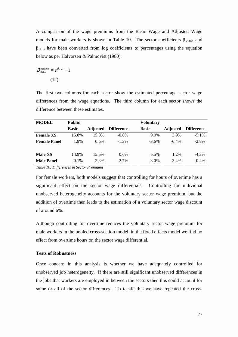
A comparison of the wage premiums from the Basic Wage and Adjusted Wage

models for male workers is shown in Table 10. The sector coefficients βVOLS and

βPUB have been converted from log coefficients to percentages using the equation

below as per Halvorsen & Palmqvist (1980).

1−= VOLSepercentVOLS

ββ

(12)

The first two columns for each sector show the estimated percentage sector wage

differences from the wage equations. The third column for each sector shows the

difference between these estimates.

MODEL Public Voluntary Basic Adjusted Difference Basic Adjusted Difference

Female XS 15.8% 15.0% -0.8% 9.0% 3.9% -5.1%

Female Panel 1.9% 0.6% -1.3% -3.6% -6.4% -2.8%

Male XS 14.9% 15.5% 0.6% 5.5% 1.2% -4.3%

Male Panel -0.1% -2.8% -2.7% -3.0% -3.4% -0.4%

Table 10: Differences in Sector Premiums

For female workers, both models suggest that controlling for hours of overtime has a

significant effect on the sector wage differentials. Controlling for individual

unobserved heterogeneity accounts for the voluntary sector wage premium, but the

addition of overtime then leads to the estimation of a voluntary sector wage discount

of around 6%.

Although controlling for overtime reduces the voluntary sector wage premium for

male workers in the pooled cross-section model, in the fixed effects model we find no

effect from overtime hours on the sector wage differential.

Tests of Robustness

Once concern in this analysis is whether we have adequately controlled for

unobserved job heterogeneity. If there are still significant unobserved differences in

the jobs that workers are employed in between the sectors then this could account for

some or all of the sector differences. To tackle this we have repeated the cross-

28

sectional estimations for two more detailed sub-industry classifications: Social Work6,

and Social Work with Accommodation.7 Although the sample size is small at the

most detailed industry level, the results were robust in both sign and significance.

The sample size at this level was too small to permit a panel estimation.

The second concern is the role of part-time working, as this is prevalent in the

voluntary sector, and affects the number of contracted hours. The model was re-

estimated using only those workers who are on full time contracts, restricting the

panel sample to 2,668 male observations and 6,537 female observations. This has no

effect on the sign or significance of the estimated effects. Furthermore, it increases

the estimated voluntary sector wage discount to 10% below the private sector wage

for female workers. The increased warm-glow estimate also supports the formulation

of warm glow utility as being related to effort rather than merely participation: the

size of this effect is bigger for workers working longer hours in the mission-motivated

organisation.

The one-year panel structure of the UK LFS is too short to be able to test for sector

differences in future job rewards resulting from overtime. The fixed effects wage

equations were estimated interacting tenure with the sector dummies, to test for sector

differences in the returns to tenure, and these coefficients were small and not

statistically significant. This does not lend support to a link between sector

differences in unpaid overtime and later within-firm rewards.

Overall, these findings suggest that there are differences in levels of unpaid overtime

between the sectors. Furthermore, for female workers the hours of unpaid overtime

support a warm-glow donated labour hypothesis, where additional hours are worked

without pay. The same is not true however for male workers. Although there are also

significant levels of unpaid overtime in the voluntary sector, controlling for these

hours does not affect the sector difference in effective hourly wage.

6 SIC Code 85.3, A sub-category of Health & Social Work 7 SIC Code 85.31, a sub-category of Social Work

29

Discussion

This paper has examined working hours and wage data from the UK Labour Force

Survey disaggregated by Industry to examine sector differentials within Health and

Social Work services, where the majority of voluntary sector workers are employed.

The empirical analysis found strong evidence of higher levels of unpaid overtime

amongst voluntary sector workers, for both males and females. The basic hours wage

equations showed a public and voluntary sector premium for both male and female

workers. This is broadly in line with the findings of Leete ( 2001) using US data.

Controlling for unobserved individual heterogeneity with a fixed effects model

accounts for the public and voluntary sector wage premiums.

The findings of this paper make two main contributions:

• The apparent nonprofit sector wage premiums in health & social work

industries are explained by unobserved worker heterogeneity;

• There are significant differences in overtime working between the sectors, and

this has an effect on sector wage differences, providing evidence of warm

glow for female workers.

Previous analysis of nonprofit wage differentials using cross-sectional data has shown

a variety of wage effects dependent on industry. The caring industries are

consistently found to have wage premiums in the voluntary and public sectors,

compared to the private sector. The analysis here shows that this can be explained

through controlling for unobserved worker heterogeneity.

Our analysis of working hours and overtime in both cross-section and panel models

supports the assertion that workers in the voluntary sector work higher levels of

overtime unpaid, while those in the private sector work more paid overtime. Two

alternative explanations for this were suggested. The first – the warm glow

hypothesis – draws on the nonprofit literature to explain higher levels of unpaid

overtime in the voluntary sector as being rewarded through intrinsic utility received

from participation in a mission-motivated activity. Therefore workers are

compensated for their ‘unpaid’ efforts through warm-glow utility.

30

The second – the gift exchange hypothesis – comes from the unpaid overtime

literature and Akerlof’s gift exchange model, suggesting that higher basic wages in

the voluntary sector compensate for the unpaid overtime. This overtime is not

explicitly contracted for, but forms part of the wage bargain and is enforced through

organisational norms. This explanation does not require any difference in the intrinsic

motivation of workers between sectors. Instead it relies on different types of

employment contract being written between the sectors to explain both the differences

in overtime patterns and basic wages.

Our findings for female workers support the warm-glow hypothesis, by showing that

effective hourly wages are lower than the private sector once unpaid overtime in

controlled for. As most workers in the voluntary sector are female, and the majority

work in the health & social work industries, this finding would explain why little

evidence of female sector wage discounts is found in studies of nonprofit wage

differentials in the wider economy. Both unobserved worker heterogeneity and unpaid

overtime must be controlled for to examine sector differences in effective hourly

wages.

However the findings for male workers differ markedly. A small and statistically

insignificant voluntary sector wage discount is found for men, and this sector wage

difference is unaffected by controlling for overtime. This would support the second

explanation – the gift exchange hypothesis – for wage-setting for male workers.

Wages for men in the voluntary sector are not significantly lowered when unpaid

overtime is controlled for.

How can we explain this apparent gender difference? It should be noted that the

voluntary sector workforce is predominantly female. As with other industries men are

disproportionally found in management roles, while the front-line care staff are more

likely to be female. This gender difference could then reflect differences in the wage

contracts written for management versus service workers. Pannenberg (2005) also

found gender differences in the compensation of unpaid overtime, with only male

workers reaping the long-run benefits of unpaid overtime. Those findings support the

assertion that male and female workers have different motives for undertaking unpaid

overtime.

31

This paper provides some evidence for warm glow in the voluntary sector. In

particular, it shows the presence of warm glow amongst female workers, a finding

absent in many other studies. It also shows the role that unpaid overtime can play in

effective wage differences. This highlights the importance of effort as a largely

unobserved variable in usual analysis of wage differentials. Hours of unpaid overtime

provide one proxy measure for effort, but more detailed study at the micro-level

would be necessary to unpick this relationship.

There is a limit to the extent that we can test hypotheses about wage contracts when

we only observe data at the individual worker level. We suggest that there is evidence

here of a difference in wage contracts by sector, but further exploration would require

the analysis of a matched employer-employee database to capture accurately

differences at the organisational level. This is the challenge for voluntary sector

research: gathering this level of detailed data on a relatively small sector is not a

trivial task. However, the recent growth of the sector, and its increasing role in the

provision of public services make it all the more important that these research

questions are addressed.

32

References

Bell, D. N. F. & Hart, R. A. (1999) "Unpaid work", Economica, vol. 66, no. 262, pp. 271-290.

Bell, D. N. F. & Hart, R. A. (2003) "Wages, hours, and overtime premia: Evidence from the British labor market", Industrial & Labor Relations Review, vol. 56, no. 3, pp. 470-480.

Bender, K. A. (1998) "The Central Government-Private Sector Wage Differential", Journal of Economic Surveys, vol. 12, no. 2, pp. 177-220.

Disney, R. & Gosling, A. (1998) "Does it pay to work in the public sector?", Fiscal Studies, vol. 19, no. 4, pp. 347-374.

Halvorsen, R. & Palmquist, R. (1980) "The Interpretation of Dummy Variables in Semi-Logarithmic Equations", American Economic Review, vol. 70, no. 3, pp. 474-475.

Hart, R. A. (2004) The economics of overtime working Cambridge University Press, Cambridge.

Heckman, J. J., Lochner, L. J., & Todd, P. E. (2006) "Earnings Functions, Rates of Return and Treatment Effects: The Mincer Equation and Beyond," in Handbook of the Economics of Education, E. A. Hanushek & F. Welch, eds., North Holland, Amsterdam, pp. 307-457.

Leete, L. (2001) "Whither the nonprofit wage differential? Estimates from the 1990 census", Journal of Labor Economics, vol. 19, no. 1, pp. 136-170.

Mocan, H. N. & Tekin, E. (2003) "Nonprofit sector and part-time work: An analysis of employer-employee matched data on child care workers", Review of Economics and Statistics, vol. 85, no. 1, pp. 38-50.

Pannenberg, M. (2005) "Long-term effects of unpaid overtime evidence for West Germany", Scottish Journal of Political Economy, vol. 52, no. 2, pp. 177-193.

Preston, A. E. (1989) "The Nonprofit Worker in A For-Profit World", Journal of Labor Economics, vol. 7, no. 4, pp. 438-463.

Ruhm, C. J. & Borkoski, C. (2003) "Compensation in the nonprofit sector", Journal of Human Resources, vol. 38, no. 4, pp. 992-1021.

Weisbrod, B. A. (1983) "Nonprofit and Proprietary Sector Behavior - Wage Differentials Among Lawyers", Journal of Labor Economics, vol. 1, no. 3, pp. 246-263.