which factors are behind germany's labour market upswing?

20|2019 Which Factors are behind Germany’s Labour Market Upswing?Christian Hutter, Sabine Klinger, Carsten Trenkler, Enzo Weber

IAB-DISCUSSION PAPERArticles on labour market issues

ISSN 2195-2663

Which Factors are behind Germany’sLabour Market Upswing?

Christian Hutter (IAB)

Sabine Klinger (IAB)

Enzo Weber (IAB, University of Regensburg)

Carsten Trenkler (University of Mannheim)

Mit der Reihe „IAB-DiscussionPaper“will das Forschungsinstitut der Bundesagentur für Arbeit denDialogmit der externenWissenscha� intensivieren. Durch die rasche Verbreitung von Forschungs-ergebnissen über das Internet soll noch vor Drucklegung Kritik angeregt und Qualität gesichertwerden.

The “IAB-Discussion Paper” is published by the research institute of the German Federal Employ-ment Agency in order to intensify the dialogue with the scientific community. The prompt publi-cation of the latest research results via the internet intends to stimulate criticism and to ensureresearch quality at an early stage before printing.

Contents

1. Introduction . . . . . . . . . . . . . . . . . . . . . . . . . . . . . . . . . . . . . . . . . . . . . . . . . . . . . . . . . . . . . . . . . . . . . . . . . . . . . . . . . . . . . . . . . . . 7

2. Data, facts, and figures . . . . . . . . . . . . . . . . . . . . . . . . . . . . . . . . . . . . . . . . . . . . . . . . . . . . . . . . . . . . . . . . . . . . . . . . . . . . . .102.1. Data . . . . . . . . . . . . . . . . . . . . . . . . . . . . . . . . . . . . . . . . . . . . . . . . . . . . . . . . . . . . . . . . . . . . . . . . . . . . . . . . . . . . . . . . . . . . . 102.2. The German labour market upswing . . . . . . . . . . . . . . . . . . . . . . . . . . . . . . . . . . . . . . . . . . . . . . . . . . . . . . . . . 11

3. Driving forces . . . . . . . . . . . . . . . . . . . . . . . . . . . . . . . . . . . . . . . . . . . . . . . . . . . . . . . . . . . . . . . . . . . . . . . . . . . . . . . . . . . . . . . . .14

4. Methodology . . . . . . . . . . . . . . . . . . . . . . . . . . . . . . . . . . . . . . . . . . . . . . . . . . . . . . . . . . . . . . . . . . . . . . . . . . . . . . . . . . . . . . . . .184.1. Model . . . . . . . . . . . . . . . . . . . . . . . . . . . . . . . . . . . . . . . . . . . . . . . . . . . . . . . . . . . . . . . . . . . . . . . . . . . . . . . . . . . . . . . . . . . . 184.2. Identification . . . . . . . . . . . . . . . . . . . . . . . . . . . . . . . . . . . . . . . . . . . . . . . . . . . . . . . . . . . . . . . . . . . . . . . . . . . . . . . . . . . 19

4.2.1. Technical identification. . . . . . . . . . . . . . . . . . . . . . . . . . . . . . . . . . . . . . . . . . . . . . . . . . . . . . . . . . . . . . . 194.2.2. Search andmatching theory . . . . . . . . . . . . . . . . . . . . . . . . . . . . . . . . . . . . . . . . . . . . . . . . . . . . . . . . . 204.2.3. Application to the SVECM . . . . . . . . . . . . . . . . . . . . . . . . . . . . . . . . . . . . . . . . . . . . . . . . . . . . . . . . . . . . 23

4.3. Specification, Estimation, and Inference . . . . . . . . . . . . . . . . . . . . . . . . . . . . . . . . . . . . . . . . . . . . . . . . . . . . 25

5. Results. . . . . . . . . . . . . . . . . . . . . . . . . . . . . . . . . . . . . . . . . . . . . . . . . . . . . . . . . . . . . . . . . . . . . . . . . . . . . . . . . . . . . . . . . . . . . . . . .285.1. Impulse Responses: What if a shock occurs? . . . . . . . . . . . . . . . . . . . . . . . . . . . . . . . . . . . . . . . . . . . . . . . . 285.2. Historical decompositions: What did the shocks e�ect over time?. . . . . . . . . . . . . . . . . . . . . . . . 325.3. Separating the e�ects of wage setting and willingness. . . . . . . . . . . . . . . . . . . . . . . . . . . . . . . . . . . . . 37

6. Conclusion . . . . . . . . . . . . . . . . . . . . . . . . . . . . . . . . . . . . . . . . . . . . . . . . . . . . . . . . . . . . . . . . . . . . . . . . . . . . . . . . . . . . . . . . . . . .40References. . . . . . . . . . . . . . . . . . . . . . . . . . . . . . . . . . . . . . . . . . . . . . . . . . . . . . . . . . . . . . . . . . . . . . . . . . . . . . . . . . . . . . . . . . . . . 41

A. Appendix . . . . . . . . . . . . . . . . . . . . . . . . . . . . . . . . . . . . . . . . . . . . . . . . . . . . . . . . . . . . . . . . . . . . . . . . . . . . . . . . . . . . . . . . . . . . . .46A.1. Details on Data . . . . . . . . . . . . . . . . . . . . . . . . . . . . . . . . . . . . . . . . . . . . . . . . . . . . . . . . . . . . . . . . . . . . . . . . . . . . . . . . . 46A.2. VECM: Specification, Estimation, and Inference. . . . . . . . . . . . . . . . . . . . . . . . . . . . . . . . . . . . . . . . . . . . . 48

A.2.1. Specification and Estimation . . . . . . . . . . . . . . . . . . . . . . . . . . . . . . . . . . . . . . . . . . . . . . . . . . . . . . . . 48A.2.2. Inference Procedures . . . . . . . . . . . . . . . . . . . . . . . . . . . . . . . . . . . . . . . . . . . . . . . . . . . . . . . . . . . . . . . . . 50

A.3. Robustness checks . . . . . . . . . . . . . . . . . . . . . . . . . . . . . . . . . . . . . . . . . . . . . . . . . . . . . . . . . . . . . . . . . . . . . . . . . . . . . 52

List of Figures

Figure 1: Employment, wages and productivity, 1992-2017 . . . . . . . . . . . . . . . . . . . . . . . . . . . . . . . . . . . . . . . . 11Figure 2: The Beveridge curve: unemployment and vacancies, 1992-2017 . . . . . . . . . . . . . . . . . . . . . . . 12Figure 3: Separation rate and job finding rate, 1992-2017 . . . . . . . . . . . . . . . . . . . . . . . . . . . . . . . . . . . . . . . . . . 12Figure 4: Impulse responses of employment . . . . . . . . . . . . . . . . . . . . . . . . . . . . . . . . . . . . . . . . . . . . . . . . . . . . . . . . 29

IAB-Discussion Paper 20|2019 3

Figure 5: Impulse responses of unemployment . . . . . . . . . . . . . . . . . . . . . . . . . . . . . . . . . . . . . . . . . . . . . . . . . . . . . 30Figure 6: Historical decomposition of employment . . . . . . . . . . . . . . . . . . . . . . . . . . . . . . . . . . . . . . . . . . . . . . . . . 33Figure 7: Historical decomposition of unemployment . . . . . . . . . . . . . . . . . . . . . . . . . . . . . . . . . . . . . . . . . . . . . . 34Figure 8: Historical decomposition of employment: pure wage setting shock and di�er-

ence to the wage determination shock of the baseline model . . . . . . . . . . . . . . . . . . . . . . . . . . 38Figure 9: Historical decomposition of unemployment: pure wage setting shock and di�er-

ence to the wage determination shock of the baseline model . . . . . . . . . . . . . . . . . . . . . . . . . . 38Figure 10: Robustness of impulse responses: Setting ξP,lf = 0. . . . . . . . . . . . . . . . . . . . . . . . . . . . . . . . . . . . . . 53Figure 11: Robustness of impulse responses: Control for statistical e�ects in F . . . . . . . . . . . . . . . . . . . 54

List of Tables

Table 1: Identifying assumptions in the matrices of short- and long-run e�ects . . . . . . . . . . . . . . . . . . . 26


Abstract

The strong and sustained labourmarket upswing in Germany iswidely recognized. In a developingliterature, various relevant studies highlight di�erent specific reasons. The underlying study, in-stead, simultaneously considers a broad set of factors in a unifiedmethodological framework andsystematically weighs the candidate reasons for the labour market upswing against each other onan empirical basis. The candidates are: shocks on (de)regulation of employment or job creationintensity, the e�iciency of the matching process, wage determination, the separation propensity,the size of the labour force, technology, business cycle and working time. We develop a struc-turalmacroeconometric framework that leaves asmanyof the systematic interlinkages aspossiblefor empirical determination while operating with a minimal set of restrictions in order to identifyeconomically meaningful shocks. For this purpose, we combine short- and long-run restrictionsbased on search-and-matching theory and established assumptions on labour force developmentand technological change. Matching e�iciency, job creation intensity, labour force, and separationpropensity yield the largest contributions in explaining the German labour market upswing.

Zusammenfassung

Der starke und anhaltende Arbeitsmarktaufschwung in Deutschland ist allgemein anerkannt. Ineiner sich entwickelnden Literatur heben verschiedene relevante Studien unterschiedliche spezi-fischeGründe hervor. Die vorliegende Studie berücksichtigt stattdessen eine Vielzahl von Faktorenin einem einheitlichen methodischen Rahmen und wägt die potenziellen Gründe für den Arbeits-marktaufschwung systematisch gegeneinander ab. Die Kandidaten sind: Schocks in Bezug auf die(De-) Regulierung der Beschä�igung oder die Intensität der Scha�ung von Arbeitsplätzen, die E�i-zienz des Matching-Prozesses, die Lohnfindung, die Entlassungsneigung, das Arbeitsangebot, dieTechnologie, den Konjunkturzyklus und die Arbeitszeit. Wir entwickeln einen strukturellenmakro-ökonometrischen Rahmen, der die Daten so frei wie möglich sprechen lässt und dabei mit einerminimalen Anzahl an Restriktionen arbeitet, um die wirtscha�lich bedeutsamen Schocks zu iden-tifizieren. ZudiesemZweck kombinierenwir kurz- und langfristige Restriktionen auf der Grundlagevon Such- und Matchingtheorie und etablierten Annahmen zur Entwicklung des ArbeitsangebotsundzumtechnologischenWandel.Matching-E�izienz, IntensitätderScha�ungvonArbeitsplätzen,Arbeitsangebot und Entlassungsneigung liefern die größten Beiträge zur Erklärung des deutschenArbeitsmarktaufschwungs.

JEL

C32, E24, J21


Keywords

German labour market upswing, labour force, job creation, deregulation, e�iciency, separationpropensity

Acknowledgements

Weare grateful to ThomasRothe and to theparticipants of the IAB-FAUMacro-Labor Seminar 2018,the IAB-UR Econometric Seminar 2019, the T2M conference 2019, the IAAE conference 2019, andthe EEA conference 2019 for helpful suggestions and valuable input.


1. Introduction

While labourmarkets in Europeandaround theworldhave struggled from the repercussions of thegreat recession and the European debt crisis for nearly a decade, Germany embarked on a strongand sustained labour market upswing. By 2018, unemployment more than halved as comparedto the peak in 2005, and employment follows a steep and stable upward trend even in times ofweak economy. Consequently, debates in academics and politics revolve around the question ofthe decisive reasons for this extraordinary development. These discussions are of high relevancefar beyond the national context, since, e.g., in Europe in particular it is considered in how far theGerman labour market reforms from the last decade should be replicated or whether the Germansuccess was based on wage dumping policies fuelling disequilibria in the EU.

In this study, we explore the empirical relevance of a comprehensive set of potential factors andweigh them against each other on the basis of a large and well-identified structural macroecono-metricmodel. Inparticular, weaddress eight shocks, namely, shockson the labour force,matchinge�iciency, separation propensity, job creation intensity / deregulation, wage determination, andworking time as well as a technology shock and a business cycle shock. This collection representsboth a synopsis and an extension of the previous literature. For example, increased matching ef-ficiency a�er severe labour market reforms has been documented (e.g., Launov and Wälde, 2016;Klinger and Weber, 2016; Hertweck and Sigrist, 2015), as well as lower separation rates (Hartunget al., 2018; Klinger and Weber, 2016). Some argue that worsened outside options increased thewillingness of the unemployed to make concessions (Krebs and Sche�el, 2013) and connect thesocial benefit reform to increased selection rates and vacancy posting (Hochmuth et al. (2019)).Others point to a positive e�ect of moderate wages and flexible wage setting (Dustmann et al.,2014). Moreover, an increase in labour supply could have boosted employment (Burda and Seele,2016) aswell as generally lowerand/ormore flexibleworkinghours (BurdaandHunt (2011), Balleeret al. (2016), Weber (2015), Carillo-Tudela et al. (2018)).

This brief review demonstrates that the literature as a whole provides an extensive debate on thesubject. Notwithstanding, the single papers usually focus on specific points. While in the courseof that many crucial points are illuminated, an investigation comprising a broad set of factors in aunified methodological framework makes a crucial contribution: By systematically weighing thecandidate reasons for the labour market upswing against each other on an empirical basis, welearn about the relevance and timing of the di�erent e�ects. This is the purpose of the underlyingstudy.

This research conceptmakes the use of a flexiblemodel approach a key issue. Particularly, it is cru-cial to choose an open approach that minimises the need of setting assumptions a priori. I.e., theless restrictive the econometric procedure is designed the more will the data speak in the results.Thereby, it is decisive that developments observed in the data are ascribed to the shocks wherethey originate. This means that the relevant shocks must be accurately filtered from the dataset,


given amultitude of potential interlinkages between the variables and their complex and dynamicstructure. This structure needs to be flexibly captured based on empirical measurement. In thisregard, a structural vector error correction (SVEC) framework has particular merits. By use of thismodel class, we can leave as many of the systematic interlinkages as possible for empirical deter-mination while operating with a minimal set of restrictions. At the same time, the model is inher-ently structural, identifying economicallymeaningful shocks. Moreover, it allows for incorporatingequilibrium e�ects.

We construct such a model for the German labour market development between 1992 and 2017comprising the stock variables unemployment, vacancies and employment, the flow variables jobfinding rate and separation rate as well as wages, productivity and working time. This set of vari-ables reasonably captures the labour market and allows for various relevant mechanisms. Weidentify the eight structural shocks mentioned above via a combination of short- and long-run re-strictions. These are based on cointegration properties, on well-established assumptions abouttechnological change and cyclical fluctuations aswell as on the search andmatching theory of thelabour market. In doing so, we demonstrate how to reconcile the theoretical search and match-ing framework with an empirical structural time series model with parsimonious restrictions. Thisadds to the growing literature that implements labour market dynamics into macro-econometricapplications (compareHairaulta andZhutova, 2018; Rahn andWeber, 2017; Nordmeier et al., 2016;Fujita, 2011; Ravn and Simonelli, 2007). Having identified the shocks, we demonstrate their labourmarket impacts in an impulse response analysis. Then, in order to assess the relevance of theshocks for the German labourmarket upswing, we conduct a historical decomposition of employ-ment and unemployment. This instrument allows tracing the labour market impact of the majordriving forces through time. In this, we consider three subperiods which are particularly relevantfor an understanding of the German labour market upswing. These are, first, the period betweenthe labour market reforms and the onset of the great recession (2005-2008), second, the great re-cession itself and the recovery therea�er (2009-2011), third, the ongoing upswing (2012-2017).

The main message is: the labour market is driven by labour market shocks themselves. Shocksthat increased job creation intensity, e.g. from deregulating the labour market, shocks that in-creased the labour force, shocks that raised the e�iciency of the matching process, and shocksthat reduced the propensity of firms to separate fromworkers yield the largest contributions in ex-plaining the German labour market upswing. While the first three shocks revealed large impulseresponse coe�icients, lower separations act via two channels: stochastically via large shocks andsystematically as the separation rate declines if the labour market becomes tighter. All in all, theresults clearly confirm a partial decoupling of the labour market from GDP or productivity devel-opment (Klinger and Weber, 2019). The cycle or technology shocks do not play a decisive role inthe overall development of employment and unemployment.

The paper proceeds as follows. Section 2 documents facts on the labour market upswing, dis-cusses the variable selection and introduces the data used in this paper. Section 3 discusses thepotential driving forces of the upswing. Section 4 presents our macroeconomic model, the identi-


fication strategy and the estimation procedure. Section 5 presents the results and the final sectionconcludes.


2. Data, facts, and figures

2.1. Data

We document the development of the German economy and labour market using eight variables:vacancies and unemployment, employment, working hours per employee and hourly wages, jobfinding rate and separation rate, as well as productivity per hour. Detailed information on the dataand summary statistics are given in appendix A.1.

We follow the labour force concept to select the labour market stocks. Therein, employment istotal employment and contains employees covered by social security, civil servants, marginallyemployed, and self-employed. Unemployment is defined following the ILO standard and is takenfrom the (European) labour force survey.

Vacancies are registered at the Federal Employment Agency (FEA). Though this number comprisesabout half of the total number of vacancies, the register data outperfom the German Job VacancySurvey regarding length and frequency of the available time series data.

The worker flow rates are calculated from a 2 percent representative sample of the IAB Employ-ment Biographies taken from the German social security and unemployment records. The datacontains all individuals who are either (1) employed subject to social security, (2) marginally em-ployed, (3) unemployment benefit recipients, (4) o�icially registered job-seekers, or (5) partici-pants in labour market policy programmes. It covers more than 80 percent of the German labourforce. To calculate the worker flows, we choose a cuto�-date each month and check for two sub-sequent months whether the employment status has changed. Employment-to-unemploymentflows are divided by the number of employees in the previous month to get the separation rate.Unemployment-to-employment flows are divided by the number of unemployed workers in theprevious month to get the job finding rate. This is consistent with the counting mechanism of theFEA: unemployment is counted in themidof amonthwhile flows fromunemployment are countedbetween that date and the mid of the following month. Previous versions of that data have beenused by Klinger and Weber (2016); Jung and Kuhn (2014); Nordmeier (2014).

Both wages and productivity are provided on an hourly basis by the system of national accountsof the German Federal Statistical O�ice. Wages contain gross wages including employers’ socialsecurity contributions. They are converted into real terms using the GDP deflator. The series onworking time is drawn from the IAB Working Time calculations. This data set summarizes surveyas well as register-based source statistics to calculate average working time per employee.

Most of the data are available at a monthly frequency. Working hours, wages and productivity,however, have to be interpolated from quarterly data. We follow Denton (1971) and use appropri-


ate anchor variables for this procedure (see appendix A.1). All data are adjusted for seasonality.The sample ranges from January 1992 to December 2017. So the total number of observationsamounts to 312.

The empirical methodology would be able to cope with stationary as well as non-stationary data.According to ADF tests, however, the null-hypothesis of non-stationarity cannot be rejected for anyof the series while it can be rejected for the di�erenced series. Hence, all variables are integratedof order I(1).

2.2. The German labour market upswing

Figures 1 to 3 document the enormous and long-lasting labour market upswing in Germany.

Figure 1.: Employment, wages and productivity, 1992-2017

-3

-2

-1

0

1

2

3

92 94 96 98 00 02 04 06 08 10 12 14 16

EmploymentWagesProductivity

Notes: Normalized monthly data. Source: Destatis. Own interpolation of wages and productivity.

Figure 1 shows employment, wages and productivity. Obviously, the steep and sustained increasein employment starting in 2006 has been accompanied by a rather moderate increase in wages.In fact, the development of wages relative to productivity implies a decrease in the labour sharemaking labour more profitable for firms than before. The behaviour of employment during thegreat recession in 2008 and 2009 has given food for debate in many developed economies. De-spite the strongest decline in GDP and productivity, Germany experienced an outstanding periodof labour hoarding, and a�er the recession, the labour market started from the level of just 2007while many other economies had to o�set large employment losses first. However, the crisis had


Figure 2.: The Beveridge curve: unemployment and vacancies, 1992-2017

.1

.2

.3

.4

.5

.6

.7

.8

1.2 1.6 2.0 2.4 2.8 3.2 3.6 4.0 4.4 4.8

Unemployment

Vaca

ncie

s

Notes: The graph shows the Beveridge curve starting in January 1992 (lower le�) and ending in December 2017 (upperle�). Unit: 1 million. Source: Federal Employment Agency (vacancies), Eurostat (unemployment).

Figure 3.: Separation rate and job finding rate, 1992-2017

0.4

0.6

0.8

1.0

1.2

1.4

3

4

5

6

7

8

9

92 94 96 98 00 02 04 06 08 10 12 14 16

Separation rate Job finding rate

Notes: Unit: percent. Source: IAB Employment Biographies. Own calculations.


le� its footprint on the development of productivity which has been sluggish since then. I.e., theGerman labour market upswing is not accompanied by a productivity upswing. Nonetheless, ex-cept for the phase of the Eurozone recession 2011-2013, GDP has been on a stable growth pathuntil the end of our sample.

Figure 2 presents the Beveridge curve, the generally downward-sloping relation between vacan-cies and unemployment. The ratio of the two is interpreted as labourmarket tightness. The figuregives important insight into the nature of the upswing: following the Hartz reforms of the years2003-2005, the curve shi�ed inwards – which has been exceptional also by international compari-son (Bova et al., 2018). The inward shi� indicates a better functioning of the labour market (com-pare Blanchard and Diamond, 1989) and has been connected to improved matching e�iciency(Klinger and Weber, 2016; Launov and Wälde, 2016). Second, starting in 2010, the curve did notshi� inwards remarkably anymore but we observe a strongly upward moving limb: The numberof vacancies relative to the unemployed has been rising extraordinarily. The labour market hasbecome unusually tight. Unemployment is no longer reduced in the same way as the stock of va-cancies increases.

The worker flow rates (Figure 3) give some intuition of why the labour market stocks improvedso much. Remarkably, the job finding rate has increased stepwise a�er the Hartz reforms. Thisincrease was shown to be of permanent, i.e., not cyclical, nature (Klinger and Weber, 2016). Evenmore strikingly, the separation rate has declined for years. By the endof our sample, it had reachedthe lowest value since reunification. As the separation ratewas found to bemore influential for thedynamics of German unemployment than job findings (e.g. Jung and Kuhn, 2014; Hertweck andSigrist, 2015; Klinger and Weber, 2016), this outstanding development also points to a potentialsource of the remarkable increase in employment and decrease in unemployment.

Undoubtedly, the figures mirror an extraordinary labour market development. Regarding OECDharmonized unemployment rates alone, Germany ranked 6 among 35 OECD countries in 2017 –while it ranked 33 in 2005. It was not for nothing that Germany had used to be called "sick manof Europe" (Siegele, 2004). The interaction of aggregate shocks and institutions (Blanchard andWolfers, 2000) has been found to be a plausible reason for the long-lasting aggravation. Hence, asimilar approach seems to be rational when explaining the reverse direction, too. Previous studiesthat investigated why the upswing occurred and, by the same token, whether it is replicable, typ-ically focus on single or a very small set of shocks or institutions. Our approach is to comprise areasonable number of driving forces in a unified empirical framework and let the data speakwhichhadwhen an influential e�ect. Not only does this approach choose from a broader set of potentialexplanations, it also allows them to interact.


3. Driving forces

We explore a broad set of potential upswing drivers. The literature so far o�en focusses on the dy-namic (labour market) outcomes following a (neutral or investment-specific) technology shock ora (fiscal or monetary) policy shock (e.g. Gali, 1999; Blanchard and Perotti, 2002; Christiano et al.,2005; Ravn andSimonelli, 2007; Rahn andWeber, 2017). Beyond their scope, however, labourmar-ket institutions themselves arehighly informative for anexplanationof the labourmarketupswing.This is even more true as the German labour market underwent many and deep institutional re-forms. Thus, applying our econometric methodology on these kinds of labour market shocks hasthemainadvantage thatweextend theusual selectionandcomprise theessential issuesdiscussedso far on our topic. In the following, we discuss the potential driving forces that are building blocksof our approach.

Labour force. A comparison of the changes in employment and unemployment during the pastdecade uncovers that the observed increase in employment cannot stem from the existing labourforce only. Burda and Seele (2016) and Klinger and Weber (2019) argue in favour of a supply sidee�ect. Indeed, while the demographic component of the German labour force is clearly negative,the labour force itself increased strongly due to record levels of net migration as well as higherparticipation. Thereby, legislative changes might have played a role. Regarding immigration, thisinvolves the enlargement of the European Union (including free movement of workers) towardsthe east. Regarding participation, reforms of the pension system raised the legal retirement ageand abolished early retirement subsidies. Thus, older workers’ incentives to staywith their firm in-creased. Beyond legal changes, the labour force rose because of refugee immigration and becausemore and more mostly female workers decided to participate, albeit o�en in part-time jobs. All inall, net migration between 2006 and 2017 amounted to 3.8 million while the participation rate ofthose aged 15 to under 65 increased from 73.7 percent in 2005 to 78.2 percent in 2017.

Working time. Given the debate on whether hours worked and employment are substitutes orcomplements, the question whether working time changes contributed to the labour market up-swing is an empirical one. In the data, two observations are specifically well documented: First,the part-time ratio – the share of part-timers in total dependent employment – rose from 34.0 per-cent in 2006 to 38.5 percent in 2017. Provided that this rise generated job-sharing in a significantmanner, the reduction in working time can be interpreted as an influential factor for employmentgrowth. Second, during the great recession in 2008/09, companies adjusted labour input along theintensivemargin: in 2009, GDP shrank by 5.6 percent, per capitaworking hours by 3.2 percent, andproductivity per hour by 2.6 percent. The extensivemargin was kept untouched on aggregate. Thelabour hoarding e�ect of slimmingworking-time accounts or subsidized short-timework schemeswere demonstrated by a large body of literature (Balleer et al., 2017, 2016; Weber, 2015; Herzog-Stein and Zapf, 2014; Burda and Hunt, 2011; Möller, 2010). This is likely to have strengthened em-ployment.


Technology. Technological change is commonly connected to supply-side shocks that improvetotal factor productivity (compare, e.g. Gali, 1999; Uhlig, 2004; Ravn and Simonelli, 2007; Rahn andWeber, 2017). Through the lens of real business cycle theory (Kydland and Prescott (1982), Plosser(1989)), technology shocks can create economic fluctuations at business cycle frequencies. Theexact pattern of e�ects of technology shocks on the labour market is subject to debate, however(Gali, 1999; Christiano et al., 2004).

Business cycle. In view of the criticism on the idea that technology shocks are the only sourceof cyclical fluctuations (e.g., Summers, 1986), we o�er a further source as an explicit cycle shock.As such, we refer to rather demand-sided drivers of economic activity, for example governmentexpenditure during the downturns. With regard to the German labourmarket upswing, argumentshave been put forward that stress the enormous economic performance of China in themid-2000scombinedwith the strong export-orientation of the German economy. However, during the periodunder consideration, the German economy experienced both stable and vivid performance aswellas the great recession and the Eurozone recession. On average, GDP rose by an annual rate of 1.5percent between2005and2017. The recent economicupswingwitnesses anunforeseenweaknessin business investment. The investment-to-GDP ratio has come down to an average of 6.7 percentsince 2009 while it was 7.7 percent before. This also points to a transitory impact rather than long-term changes in productivity or potential growth.

Wage determination. The potential influence of wage determination on labour market outcomesis straightforward. The sources and the mechanisms, however, may be manifold: First, considerthe wage moderation a�er reunification when large parts of the Eastern German economy turnedout to be unproductive and had to face new competitors form the Eastern European transitioneconomies (Dustmann et al., 2014). Second, wage setting institutions have becomemore flexible.Collective bargaining coverage in Western Germany has decreased from 57 percent in 2006 to 49percent in 2017 (IAB Establishment Panel). Opening clauses in collective bargaining contracts easethe adjustment process over the business cycle (also Dustmann et al., 2014). Wage concessionsby workers were observed during the great recession (Heckmann et al., 2009). Third, with risinglabourmarket tightness, wage concessions by firms have becomemore important as compared tothe period before the upswing (German Job Vacancy Survey). Fourth, the introduction of a generalminimum wage in 2015 increased reservation wages and made wage setting less flexible again.It a�ected about 10 percent of all employees (Bossler, 2017), but a di�-in-di� analysis revealedonly limited short-run e�ects on employment (Caliendo et al., 2018). Fi�h, workers’ outside op-tions worsened remarkably. The Hartz reform reduced the entitlement period to unemploymentbenefit. It introduced sanctions when unemployed did not meet the targeted search e�ort. It es-tablished a means-tested social assistance system that led to an immediate reduction of the netreplacement rate by 11 percentage points between 2004 and 2005; between 2003 and 2011, the re-placement rate even dropped by 20 percentage points. Worse outside options reduce reservationwages and bargaining power of workers. Hence, workers’ willingness to make (wage) concessionshad increased a�er the Hartz reforms (Krebs and Sche�el, 2013; Rebien and Kettner, 2011). In gen-eral, our term "wage determination" comprises both the wage setting process and the willingness


to make concessions or increase search intensity according to the outside options. In subsection5.3, we will separate these two ingredients.

Matching e�iciency. Regarding the e�iciency of the matching process we disentangle e�iciencyconnected to search intensity and e�iciency connected to the matching technology itself, i.e. thetechnological toolkit and institutional framework for unemployed, firms and the public employ-ment service to form matches. Search intensity is already captured by wage determination (seeoutside options above). Regarding the matching technology itself, online job platforms, also in-troduced by the FEA, contributed to increased market transparency and improved matching. Fur-thermore, the FEA and its local branches underwent a severe restructuring of its organisation andtasks in the course of the Hartz reforms. Since 2004, the FEA has been providing measures of ac-tive labour market policy according to the principles of e�ectiveness and e�iciency. Social ben-efit recipients were included in the labour market policy e�orts. Furthermore, it introduced casemanagers and a customer segmentation to tailor treatment properly and established specific ser-vice departments for firms. All this targeted at reducing mismatch and imperfect information. In-deed, an increase of matching e�iciency a�er the reforms has been documented by, e.g., LaunovandWälde (2016); Klinger andWeber (2016); Stops (2016); Hertweck and Sigrist (2015); Klinger andRothe (2012); Fahr and Sunde (2009). Nonetheless, the worse the searcher profiles become in thecourse of a strong reduction in unemployment, the harder it is tomaintain or even further increasematching e�iciency.

Separation propensity. The role of separations in explaining the labour market upswing in Ger-manyhasbeenaddressedbyKlinger andWeber (2019, 2016) andHartunget al. (2018). Thepropen-sity of firms to dismiss workers depends on firing costs on the one hand and on the opportunitycosts of firing and rehiring on the other hand. The most relevant source of changes in firing costsare changes in the employment protection legislation (EPL). Indeed, the OECD indicator on thestrictness of employment protection in temporary contracts shrank from 3.25 at the beginning ofthe 1990s to 1.13 since 2013. In the course of theHartz reforms, negotiation of fixed-term contractswasmade easier and theminimum firm size for which the standard EPL applies was raised. Relax-ing EPL (or allowing fixed-term contracts) typically increases job creation and labourmarket flowsbuthashardly anye�ectonemploymentandunemployment (Kahn, 2010;CahucandPostel-Vinay,2002). As regards the second aspect, opportunity costs of firing and rehiring are a�ected by labourmarket tightness. The more costly and time-consuming the hiring process is, the more cautiousare firm’s firing strategies.

Job creation intensity. Job creation intensity determines vacancy posting beyond the scope thatstandard fundamental factors of a job creation curve – such as productivity, wage costs andmatch-ing rate – account for. For instance, Gehrke andWeber (2018) isolate such ameasure of job creationintensity fromsystematic vacancypostingexplainedby the factorsmentionedabove. This is equiv-alent to the e�iciency parameter in a matching or production function. Notably, labour marketderegulation enters job creation intensity because it lowers the costs to obey legal restrictions inemployment contracts. In Germany, temporary agency work as well as marginal employment ac-


counted for a substantial part of the labour market dynamics a�er they had been deregulated bythe Hartz reforms. Regarding temporary agency work, the government abolished limits of assign-ment duration, made it easier to rehire, and allowed for own collective bargaining instead of equalpay (in 2018, some of these elements were removed). The share of temporary agency workers intotal employment covered by social security has more than doubled from 1.2 percent in 2004 to2.7 percent in 2017. The share in total incoming vacancies increased from 21.3 percent in 2005 to34.4 percent in 2017 (earlier comparable data is not available). Regarding marginal employment,the tax and social contribution burden was lowered and the working time limit was abolished.(Nonetheless, marginal employment contains not even 30 percent of a full-time contract on aver-age). Within the first four years a�er the reform, the number of marginally employed rose bymorethan 10 percent. Since then, it has been declining.

In the next section, we present the econometricmodel to explore when and howmuch the diversedriving forces a�ected the German labour market.


4. Methodology

4.1. Model

As a precondition of reliable impulse responses and a meaningful historical decomposition, ourmodel combines two properties: First, it is structural in that economically meaningful shocks areidentified and equilibrium e�ects can be considered. Second, it captures very general dynamicsand interaction of the variables without imposing strong structural assumptions a priori. In fact,the task of the model structure is to provide a suitable econometric frame to let the data speak.Thus, we start with a vector autoregressive process of order q, VAR(q):

yt =

q∑i=1

Aiyt−i + µDt + ut, t = 1, 2, . . . , T, (4.1)

where yt = (y1t, . . . , yKt)′ is a K-dimensional random vector, Ai are fixed (K × K) coe�icient

matrices, andDt = (1, t)′ collects the deterministic terms with associated fixed coe�icients µ =

(µ0, µ1), where µi, i = 0, 1, is of dimensionK × 1. To ensure asymptotic validity of our inferenceprocedureswe assume thatut is aK-dimension iid processwith E(ut) = 0, E(utu

′t) = Σu,Σu being

nonsingular, and, for some finite constant c, E|uitujtuktumt| < c for i, j, k,m = 1, . . . ,K, and all t.Finally, the initial values y0, . . . , y−q+1 are assumed to be fixed.

In our case, yt contains theK = 8 endogenous variables vacancies (V ), unemployment (U ), em-ployment (E), job finding rate (F ), wages (W ), productivity (P ), separation rate (S) and workingtime per employee (H). This choice of variables reflects the unified economic framework of labourmarket stock and flow variables necessary to investigate our research questions.

AugmentedDickey-Fuller (ADF) tests confirmthatourvariables shouldbe treatedasnon-stationary,i.e., the VAR process is assumed to be integrated of order 1. This implies, first, the existence of non-zero long-run e�ects of the shocks and, second, the potential presence of cointegration relation-ships among the variables. These relationships may represent equilibrium e�ects in the modeleconomy. Therefore, we re-write the VAR (4.1) into a vector error correctionmodel (VECM) that ex-plicitly incorporates the cointegration relationships as preferredby the data. The considered VECMreads as

∆yt = ν + αβ′(yt−1 − ρ1(t− 1)) +

q−1∑i=1

Γi∆yt−i + ut, (4.2)

whereΓi = −∑q

j=i+1Aj , i = 1, . . . , q−1, andΠ = −(IK−A1−· · ·−Aq)with 0 ≤ rk(Π) = r < K

such thatΠ = αβ′ with α and β being full column rank (K × r)matrices for 0 < r < K. Note thatr is equal to the number of linearly independent cointegration relations given by β′yt−1. We haveassumed that µ1 = −αβ′ρ1 for some deterministicK × 1 vector ρ1. Hence, the linear trend can be


restricted to the cointegration relations such that the VAR process does not allow for a quadratictrend, compare Johansen (1995: Sect. 5.7). It follows that ν = µ0 − αβ′ρ1.

The VECM (4.2) represents the reduced form of an underlying structural system. In particular, thecontemporaneously correlated residuals in ut do not represent economically interpretable inno-vations. Instead, they are usually specified as linear combinations of unique structural shocks.Formally, this can be expressed as

ut = Bεt, (4.3)

where B is a nonsingular (K × K) coe�icient matrix such that Σu = BB′, and εt represents thevector of structural shocks. Our approach connects these shocks to the driving forces discussedabove.

By inserting (4.3) into (4.2) we obtain the structural VECM (SVECM). From this SVECM, we obtainunder appropriate assumptions, compare Johansen (1995: Theorem 4.2), the following structuralmoving average (MA) representation for yt

yt = Ct∑i=1

(Bεi + µDt) + C(L)(Bεt + µDt) +A, (4.4)

where A depends on initial values such that β′A = 0, C = β⊥(α′⊥(Ik −∑q−1

i=1 Γi)β⊥)−1α′⊥ withα⊥ and β⊥ being (K × K − r) matrices of full column rank such that α′α⊥ = 0 and β′β⊥ = 0,respectively. Moreover, C(L)Bεt =

∑∞i=0Ciut−i is an I(0) process. The coe�icient matrices Ci,

i = 0, 1, 2, . . ., depend on the VECM parameters and it holds thatCi → 0 as i→∞.

Hence, the long-run e�ects of the structural shocks on the model variables in yt are given by theso-called long-run impact matrix CB. Moreover, (C + Ci)B represents the structural impulse re-sponses at any finite horizon i with C + C0 = IK such that B contains the impact e�ects of theshocks. Finally, note that CB is of reduced rankK − r. Thus, the long-run impulse responses ofthe variables are not linearly independent if r > 0.

4.2. Identification

4.2.1. Technical identification

As is well known, the initial impact matrix B, i.e., the SVECM, is not identified without imposingrestrictions. AssumingE[εtε

′t] = IK by convention, we need to impose at leastK(K − 1)/2 = 28

(linearly) independent restrictions on B and CB to achieve identification, see Lütkepohl (2005:Sect. 9.2). Restrictions on B will be called short-run restrictions while restrictions on CB are la-


beled as long-run restrictions. AsCB is of reduced rank in case of cointegration one has to be care-ful when determining the number of independent restrictions. For example, a zero column inCBonly counts forK − r independent restrictions, for a discussion see Lütkepohl (2005: Sect. 9.2).

In our empiricalmodel set-upwe impose exactly 28 linear restrictions. Based on our estimates, therank criterion of Lütkepohl (2005: Proposition 9.4) indicates local identification of the SVECM, i.e.,the existence of a locally unique solution for B. Identification is only local asB enters Σu = BB′

in ”squared form”. Hence, identification is only up to column signs as multiplying a column of Bwith −1 will still recover Σu. To obtain a globally unique matrix B, we follow Lütkepohl (2005:Sect. 9.1.2) and normalize one element in each columnofB to be non-negative. In detail, we applythe following sign normalizations with respect to the structural shocks described below: job cre-ation intensity shock on vacancies, labour force shock on the sum of employment and unemploy-ment, wage shock on wages, e�iciency shock on the job finding rate, cycle shock and technologyshock on productivity1, separation propensity shock on the separation rate, working time shockon hours.

In order to identify these economically meaningful shocks, we eventually apply an identificationscheme that distinguishes the shocks by when, how, and how long they hit the model economy.Our econometric framework has the advantage of leaving the dynamics completely unrestrictedand introducing constraints on the immediate and/or the long-run impact only to the extent thatis necessary and economically justifiable. Thereby, the short- and long-run restrictions are basedon well-established assumptions on technological change or the business cycle as well as on thesearchandmatching theoryof the labourmarket. In the following, the latter is laidout in abaselinemodel version on which we can draw when detailing the identification.

4.2.2. Search andmatching theory

The search andmatching approach (Diamond, 1982; Mortensen and Pissarides, 1994) contains thefollowingmain features: We explicitly consider two labourmarket states, employedEt and unem-ployed Ut. The respective shares in the labour force Lt would add to 1.

UtLt

= 1− EtLt

(4.5)

In addition, a third state, out of the (domestic) labour force, is taken into account as the labourforce (employment plus unemployment) is allowed to be time-varying.

Either state evolves through the lawofmotion. The change in employment, for example, originates

1 The cycle shock loads positively also on other variables such as employment or hours, so that the choice of nor-malisation has no e�ect here.


from separations St andmatchesMt:

∆Et = Mt − St (4.6)

Search for a job or aworker, respectively, is costly and time-consuming. Search frictions arise fromasymmetric information,mismatch, and the lackof a centralmarketplace. Matchesare formedoutof vacancies Vt and unemployedUt according to amatching function, i.e. the production functionof matches (in this case, with constant returns to scale).

Mt = µtV1−αt−1 U

αt−1 (4.7)

Matching e�iciency µt represents the productivity measure of that function. It depends on deter-minants such as the institutional quality of employment services, search intensity, willingness totakeupwork, ormismatch (compareLaunovandWälde, 2016;KlingerandWeber, 2016;Davis et al.,2013).

The structure of job seekers could be further controlled for by inserting exogenous variables intoa vector Xt that account for the shares of, among others, the long-term unemployed or the low-qualified in total unemployment (e.g. Gehrke and Weber (2018)).

µt = µ∗t +Xtβ (4.8)

Thestockvariablesenter thematching functionwithone lag,whichaccounts for theexpenditureoftime that the whole search and recruiting process takes and is consistent with the countingmech-anism of the FEA (see section 2.1). Regardingmonthly data, the time aggregation bias is negligiblysmall (Nordmeier, 2014). As a consequence of this timing, the job finding rate will react on impactonly to shocks that directly a�ect matching e�iciency but not to shocks that change only unem-ployment and vacancies in the first round.

The job finding rate jfrt and the worker finding rate wfrt relate matches to the lagged stocks ofunemployment and vacancies, respectively. With labour market tightness defined as θt = Vt/Ut,they read as:

jfrt =Mt

Ut−1= µtθ

1−αt−1 (4.9)

wfrt =Mt

Vt−1= µtθ

−αt−1 (4.10)


Free entry of firms is ensured. This yields a job creation curve of the form:

κV

wfrt= pt − wt + δ(1− st)

κV

wfrt+1, (4.11)

where κV is named vacancy posting costs and comprises all sorts of costs that a�ect the value ofa (vacant or filled) job, such as recruitment costs or legal obligations connected to the job. pt andwt are productivity gained from and wages paid for the match. st equals the total separation rateand comprises exogenous as well as endogenous separations.

Amatchof a vacancy andanunemployedperson creates a surplus. Forworkers, the resultingwageexceeds the value of outside options like unemployment benefit or home production b while forfirms, the profit from the productivematch exceeds the value of a vacant job. The surplus is sharedinwage negotiations according to a Nash bargaining rule where bargaining power γ of either partyand reservation wages become relevant.

wt = γ(pt + θt−1κV ) + (1− γ)b (4.12)

Separations consist of a group of exogenous dismissals or quits and a group of endogenously dis-missed workers (compare Fujita and Ramey, 2012). Exogenous separations occur with separationrate sext (which is time-varying because it may be subject to shocks). Endogenous separations oc-cur because i) a worker’s productivity is hit by an idiosyncratic shock with arrival rate λ that leadsto a new productivity below reservation productivity with probabilityG(R) or ii) reservation pro-ductivity changes such that a fraction ofworkersEt−1(Rt)/Et−1 is a�ected even if they do not facea productivity shock (expressed by the complementary probability (1− λ)Et−1).

St = sext Et−1 + (1− sext )(λG(Rt)Et−1 + (1− λ)Et−1(Rt)) (4.13)

Reservation productivity is derived from the endogenous job destruction condition (Pissarides(2000)). A job is destroyed if its value is zero, i.e. if its return (productivity minus wages) is toolow:

0 = pR− w(R) +λ

δ + λ

1∫R

[p(n−R)− (w(n)− w(R))] dG(n) (4.14)

Conclusively, the theory postulates relations between variables none of which is restricted in themodel, not even on impact. The details which e�ects we may restrict are given below. Table 1presents an overview.


Table 1.: Identifying assumptions in thematrices of short- and long-run e�ects

responseshock lf wt tech cyc wd e� sep jci

Short runvacancies θV,lf θV,wt θV,tech θV,cyc θV,wd θV,eff θV,sep θV,jciunemployment θU,lf θU,wt θU,tech θU,cyc θU,wd θU,eff θU,sep 0employment θE,lf -θU,wt -θU,tech -θU,cyc θE,wd -θU,eff -θU,sep -θU,jci

job finding rate 0 θF,wt θF,tech θF,cyc θF,wd θF,eff 0 0wage θW,lf θW,wt θW,tech θW,cyc θW,wd 0 θW,sep θW,jci

productivity θP,lf θP,wt θP,tech θP,cyc θP,wd θP,eff θP,sep θP,jci

separation rate θS,lf θS,wt θS,tech θS,cyc θS,wd 0 θS,sep 0working time 0 θH,wt θH,tech θH,cyc θH,wd 0 0 0

Long runvacancies ξV,lf ξV,wt ξV,tech 0 ξV,wd ξV,eff ξV,sep ξV,jciunemployment ξU,lf ξU,wt ξU,tech (0) ξU,wd ξU,eff ξU,sep ξU,jci

employment ξE,lf ξE,wt ξE,tech (0) ξE,wd ξE,eff ξE,sep ξE,jci

job finding rate ξF,lf ξF,wt ξF,tech 0 ξF,wd ξF,eff ξF,sep ξF,jci

wage ξW,lf ξW,wt ξW,tech 0 ξW,wd ξW,eff ξW,sep ξW,jci

productivity ξP,lf 0 ξP,tech 0 0 0 0 0separation rate ξS,lf ξS,wt ξS,tech 0 ξS,wd ξS,eff ξS,sep ξS,jciworking time ξH,lf ξH,wt ξH,tech 0 ξH,wd ξH,eff ξH,sep ξH,jci

Notes: The table shows the identifying assumptions regarding the short- and long-run e�ects in our structuralmacroe-conometric model. lf: labour force, wt: working time, tech: technology, cyc: business cycle, wd: wage determination,e�: matching e�iciency, sep: separation propensity, jci: job creation intensity. θk,j and ξk,j are defined as the contem-poraneous and long-term reactions of the kth variable to the jth structural shock, respectively. (0): Two of the eightcycle shock zeroes are no additional binding restrictions, but zeroes that follow from the cointegration properties.


4.2.3. Application to the SVECM

Labour force shock. Once workers have entered the labour force, they are either employed orunemployed (equation 4.5). Then, changes to employment are equivalent to changes in unem-ployment with opposite sign, at least on impact. The labour force shock – e.g. higher immigra-tion or participation – changes the size of the work force. It is the only one that can immediatelya�ect the labour force and may thus move both employment and unemployment into the samedirection (for exceptions see below). The labour force shock may make additional persons enterunemployment, but sincematches by definition of thematching functionwould appear only fromthe following month onwards (equation 4.7), there is no contemporaneous e�ect on the job find-ing rate. In the long run, one could think of the labour force shock as a pure blow-up of the labourforce, corresponding to a blow-up in vacancies leaving labourmarket tightness and the job findingrate as well as the separation rate una�ected. By the same token, one might restrict the long-runresponses of wages and productivity, too. Since these restrictions are not necessary for full iden-tification and would considerably decrease the likelihood, we leave these e�ects unconstrained.This allows for heterogeneity in the composition of the additional labour force and also has theadvantage of not a priori excluding specific results from the migration literature (e.g., Ottavianoand Peri, 2012). However, appendix A.3 shows that the results do not hinge on this exception.

Working time shock. This shock – for example variations in the part-time ratio or the facilitation ofshort-timework during the great recession – is the only one to changeworking hours per employeeimmediately (for exceptions seebelow). Note that a shock refers to an innovation that goesbeyondendogenous reactions. If, for example, working time decreases in a recession in just the usual way,the cause is not a working time shock itself but a shock to economic activity.

Technology shock. The technology shock is the only one to a�ect labour productivity in the longrun, following the standard assumption by Gali (1999) and many others. The only exception is thelabour force shock as explained above. With respect to the short run, only the restriction of a con-gruent development of employment and unemployment applies (equation 4.5). In particular, weallow a free estimate of the responses of working hours on impact as well as in the long run (thisis an exception to the identifying rule of the working time shock). Given the discordant literatureon how technology shocks a�ect total hours worked (e.g. Uhlig, 2004; Canova et al., 2010), an un-restricted empirical strategy seems reasonable. Accordingly, the reaction of employment is unre-stricted, which follows directly from the job creation and job destruction equations (4.11), (4.13)and (4.14). However, we show in appendix A.3 that the results are robust to this exception.

Cycle shock. The cycle shock is allowed to produce economic fluctuations at business cycle fre-quencies but does not a�ect the economy in the long run. Hence, the column in thematrix of long-run e�ects CB referring to the cycle shock is set to zero. This zero column only counts forK − rindependent restrictions as r of the zero entries are an implicit consequence of the cointegrationproperties as discussed above. On impact, the cycle shock is exempted from the identifying rule of


the working time shock. Instead, an immediate reaction of working time is allowed in order to ac-commodate results that demand shocks are mitigated along the intensive margin (e.g. Panovska(2017), Herzog-Stein and Zapf (2014)).

Wage determination shock. The wage determination shock is the only one that immediately af-fects all variables. This generous identification scheme is rationalized as the shock summarizesseveral sources why wages initially change (see section 3), among them wage bargaining, wageconcessions, minimum wage reforms, outside options and reservation wages. This collection isjustified by the Nash bargaining rule of the search andmatchingmodel (equation 4.12): Wages arenegotiated to optimally share the surplus from the match between workers and firms. They de-pendon thebargainingpowerand theoutsideoptionsofworkers (aswell asproductivity and tight-ness which refer to other shocks of our model). However, the collection demands a strict schemewhere to impose a zero restriction. Wage concessions may influence firms’ separation decisions(equation 4.14). Besides the extensive margin of labour demand (E), our baseline model also al-lows for contemporaneous e�ects on the intensive margin (H). Outside options and reservationwages impact job findings immediately via matching e�iciency, if a (low-paid) job is more quicklyaccepted (equation 4.8). Moreover, wage shocks following changes to labour market institutionsdo not solely enforce adjustments within the labour force but may even prompt agents to enteror leave the labour force (Rothe and Wälde, 2017; Fuchs, 2014). Besides this broad definition ofa wage determination shock, subsection 5.3 provides the results of an alternative identificationstrategy allowing us to separate the pure wage setting channel and the willingness channel of thisshock.

Matching e�iciency shock. The matching e�iciency shock refers to the functioning of the labourmarket beyond job search intensity and includes, for example, changes to the transparency and in-stitutions of thematchingprocess. The e�iciency shock a�ects thematching technology (equation4.7) – immediately moving the job finding rate, employment and vacancies (equations 4.9 and 4.6and 4.11). We refrain from immediate impacts of the e�iciency shock onwages and the separationrate, asmatches do not showup contemporaneously in thewage equation (4.12) nor in the job de-struction equations (4.13) and (4.14). The restrictions hold even if wewould assume that e�iciencya�ects hiring costs which might imply a short-run e�ect on wages and separations. But empiricalstudies find hiring costs to be low (Carbonero and Gartner, 2017), so their changes would be of asize of secondary importance. Moreover, the share passed toworkers throughwage renegotiationsis likely to be limited, and the e�ect on the averagewage level of all employees is negligible. By thesame token, the option value of labour hoarding in the reservation productivity (the cut-o� pointfor separations, see equation 4.14) would not be changed considerably.

Separation propensity shock. A separation propensity shock – for example changes in firing costs– moves the separation rate irrespective of other endogenous factors such as labour market tight-ness. The slow-down of the separation rate due to increased labour scarcity would be found inthe systematic reactions of themodel to changes in vacancies and unemployment. As regards thestochastic separations propensity shock, it changes the option value of a job in case of split-up. Via


jobcreation (equation4.11), tightness reacts. Butmatchinge�iciency isuna�ected, so thee�ectonthe job finding rate is zero on impact (equation 4.7). Furthermore, the rules identifying the labourforce and the working time shocks are binding. As the bargaining power of workers is a�ected bythe readiness for dismissals (depending on employment protection, fixed-term contracts, rehiringcosts etc.) wages may well be renegotiated, and this e�ect is le� unrestricted (equation 4.12).

Job creation intensity shock. A job creation intensity shock increases vacancy posting beyond theinfluenceof standard factors suchaswagesandproductivity. The relevant shi�ingparameter in thejob creation equation (4.11), named vacancy posting costs, comprises recruitment costs as well ascosts connected toany legal regulations for, e.g., temporary agencywork. Thus, sucha shock couldchange the flexibility of employment contracts on the brink of the labour market by deregulation,for example. It a�ects thevalueof (such) jobs for firmswhich increases vacancies and tightnessandraises the job finding rate (equation 4.9), but – according to thematching function (4.7) – only withdelay. There might be an increase in matching e�iciency, because for given tightness, the shareof vacancies for temps with comparatively low duration rises. This increases the average workerfinding rate and, consequently, the job finding rate – but also with delay as this kind of vacancieshas tobe created, and filled, first. By the same token, the separation rate cannot react immediately:vacancies have to be created and filled before the new match can be separated. With job findingrate and separation rate being constant on impact, the law of motion (4.6) implies a zero e�ect forunemployment, too.

4.3. Specification, Estimation, and Inference

In order to avoid serial correlation in the reduced form residuals, we consider a VAR order of q = 7,even though the information criteria (Akaike, Bayesian) would have preferred fewer lags.

Based on the VAR(7) we run the so-called trace test, see Johansen (1995), and find r = 2 coin-tegration relations. Cointegrations relations generalize a VAR in first di�erences. Thus, in the firstplace, we specify these two cointegration relations to bring themodel as close to the data as possi-ble. Beyond that, the search andmatching theory gives rise to believe that such long-run relationseconomically exist (think, for instance, of the Beveridge curve or the job creation curve). However,restricting the cointegration space to specific relationships is not necessary for our purposes. Al-lowing for r = 2, we use Johansen’s maximum likelihood (ML) approach to estimate the reducedform VECM parameters in (4.2) including the cointegration matrix β.

In order to take into account equation (4.8) and control for shi�s in µt due to a changing compo-sition of the unemployed, we add as exogenous variables the following five shares with respectto all unemployed persons to the equation for the job finding rate in our VECM: low-skilled (nocompleted degree), long-term (> 1 year), old (aged 55+), foreign, female.


We apply a sequential elimination procedure based on a restricted feasible GLS (FGLS) estimator,see Lütkepohl (2005: Sects. 5.2 and 7.3), to find a parsimonious subset VECM. To be precise, we se-quentially exclude the short-run dynamics parameters inΓi, i = 1, . . . , q− 1, that do not satisfy anabsolute t-value of at least 1.645. This threshold value is consistent with a 10 percent significancelevel based on the standard normal distribution. The adjusted Portmanteau test, see, e.g., Lütke-pohl (2005: Sect. 8.4.1), cannot reject the null hypothesis of no serial correlation in the residuals ofthe resulting subset VECM up to lag 24 even at the 10 percent significance level.

Following Lütkepohl (2005: Sect. 9.1), the structural form is estimatedusing anon-linearmaximumlikelihood approach employing the restrictions introduced in section 4.2. Inference on the impulseresponses shown in the next section is based on a semiparametric bootstrap approach that deliv-ers the displayed pointwise confidence intervals. We describe our specification, estimation, andbootstrap approaches in more detail in Appendix A.2.


5. Results

5.1. Impulse Responses: What if a shock occurs?

Having identified the structural shocks, wedemonstrate their labourmarket impacts in an impulseresponse analysis. Impulse responses have the character of a hypothetical simulation: They showthe reactions of the model variables over time if a specific shock occurs. We present the resultswith respect to employment and unemployment as the two key variables of the labour marketupswing.1 They are given in Figures 4 and 5 together with 2/3 bootstrapped confidence intervalsthat are calculated following Hall (1992). The impulse responses are comparable in size since allshocks are normalised to have a variance of 1. The scale unit in the figures is 1 million.

Both employment and unemployment increase significantly following a unit labour force shock.Thee�ectonunemployment is comparatively small andbecomes insignificantwithin the first year.This result resembles the finding in the macro-econometric study by Weber and Weigand (2018)who conclude that immigration to Germany did not raise unemployment.2 Employment, by con-trast, reacts rather quickly and reaches a significant total e�ect of about 60,000workers. The quickreactionof employment to labour force shocks is in linewithBlanchard (2006). Weargue thatwhenthe labour force increases due to later retirement age, for instance, unemployment is not a�ectedat all. With increasing employment and stable unemployment, the unemployment rate will shrinkin the long run due to a positive labour force shock.

A positive working time shock by one unit decreases employment by 40,000 and increases un-employment by more than 20,000 people in the long run. Both e�ects are significant. From themacroeconomic point of view, working hours and workers are substitutes. Thus, working time re-ductions during the great recession via working time accounts or publicly subsidized short-timework could have helped to hoard labour. The reaction is sluggish, however, possibly because ittakes more time to adjust workers than to adjust working hours. Furthermore, if the short-timework scheme had not existed during the great recession, firms would have dismissed more work-ers – but certainly not at once but distributed over several months.

In the short-run, the technology shock has only a small impact on unemployment and employ-ment. Over time, however, the e�ects lead to significant increases in employment and reductionsin unemployment by about 40,000people. This pattern accounts for a remarkable adjustment pro-cess where technological progress creates new job opportunities in the long-run.

A positive one unit cycle shock represents an economic expansion. It has a positive impact onproductivity but not as strong as the technology shock. Consequently, the “cyclical” reactions are

1 The impulse responses of the other variables have been checked for plausibility and are available upon request.2 Our labour force shock does not only include immigration, but also participation and demographics.


Figure 4.: Impulse responses of employment

.00

.02

.04

.06

.08

.10

0 4 8 12 16 20 24 28 32 36 40 44 48

Labour force shock

-.14-.12-.10-.08-.06-.04-.02.00.02

0 4 8 12 16 20 24 28 32 36 40 44 48

Working time shock

.00

.01

.02

.03

.04

.05

.06

.07

.08

0 4 8 12 16 20 24 28 32 36 40 44 48

Technology shock

-.008

-.004

.000

.004

.008

.012

0 4 8 12 16 20 24 28 32 36 40 44 48

Cycle shock

-.06-.05-.04-.03-.02-.01.00.01.02

0 4 8 12 16 20 24 28 32 36 40 44 48

Wage determination shock

.00

.02

.04

.06

.08

.10

.12

.14

0 4 8 12 16 20 24 28 32 36 40 44 48

Efficiency shock

-.05

-.04

-.03

-.02

-.01

.00

0 4 8 12 16 20 24 28 32 36 40 44 48

Separation propensity shock

-.02.00.02.04.06.08.10.12.14.16

0 4 8 12 16 20 24 28 32 36 40 44 48

Job creation intensity shock

Notes: The solid lines show the responses of employment to 1 unit shocks up to 48 months. The dotted lines denoteHall (1992)’s 2/3 bootstrapped confidence intervals. Unit: 1 million. Source: Own calculations.


Figure 5.: Impulse responses of unemployment

-.025-.020-.015-.010-.005.000.005.010.015

0 4 8 12 16 20 24 28 32 36 40 44 48

Labour force shock

-.02

.00

.02

.04

.06

.08

.10

0 4 8 12 16 20 24 28 32 36 40 44 48

Working time shock

-.07

-.06-.05

-.04-.03-.02

-.01.00

0 4 8 12 16 20 24 28 32 36 40 44 48

Technology shock

-.010

-.008-.006

-.004-.002.000

.002

.004

0 4 8 12 16 20 24 28 32 36 40 44 48

Cycle shock

.00

.01

.02

.03

.04

.05

.06

.07

.08

0 4 8 12 16 20 24 28 32 36 40 44 48

Wage determination shock

-.14

-.12-.10

-.08-.06

-.04-.02

.00

0 4 8 12 16 20 24 28 32 36 40 44 48

Matching efficiency shock

.00

.01

.02

.03

.04

.05

0 4 8 12 16 20 24 28 32 36 40 44 48

Separation propensity shock

-.12

-.10

-.08

-.06

-.04

-.02

.00

0 4 8 12 16 20 24 28 32 36 40 44 48

Job creation intensity shock

Notes: The solid lines show the responses of unemployment to 1 unit shocks up to 48months. The dotted lines denoteHall (1992)’s 2/3 bootstrapped confidence intervals. Unit: 1 million Source: Own calculations.


small (just as documented by Klinger andWeber (2019) on the decoupling of employment growthfrom the business cycle). In the long-run, both e�ects turn to zero by restriction. These impulseresponses have the following implications: First, persistent changes in employment and unem-ployment are assigned to the technology shock. Second, it needs large shocks for the cycle to bea potential driver of the labour market upswing. However, the small e�ects might turn out advan-tageous if the great recession is classified as a negative cycle shock (see next section).

The impulse responses of thewage determination shock show significant harmful e�ects follow-ingwage increases. Unemployment continuously rises up to a long-run e�ect of about 40,000 peo-ple. Employment slightly rises on impact but then turns negative until it reaches a long-run e�ectof about 30,000 workers less. Furthermore, higher wages reduce the number of vacancies and thejob finding rate. Vice versa, negativewage shocksmay well have contributed to the labourmarketupswing.

Highly significant andeconomically relevant e�ects are visible followingaunitmatchinge�iciencyshock: Unemployment and employment are a�ected similarly. They steadily decline/rise until thelong-run e�ect of approximately 90,000 people less in unemployment and 80,000 people more inwork is reached. Matching e�iciency amounts to one of the largest single e�ects in this impulse-response analysis, rationalising the assumption that the parts of the Hartz reforms that increasedmatching e�iciency were an influential driver of the labour market upswing. One reason for itsstrong e�ects ist that higher matching e�iciency also raises the number of vacancies and the jobfinding rate while it decreases the separation rate.

A positive separation propensity shock, as initiated by a decrease in employment protection (an-other issue of the Hartz reforms), worsens labour market stocks significantly by about 30,000 inthe long-run. In line with the EPL literature, labour market dynamics rise, though the job findingrate only temporarily. Vice versa, a negative separation propensity shock increases employmentvia fewer exits and reduces unemployment via fewer entries.

Finally, a job creation intensity shock has large positive e�ects on the labour market. Accompa-nied by increases in vacancies and the job finding rate, employment rises following a positive jobcreation intensity shock by about 90,000 workers in the long-run, while unemployment decreasesby about 80,000 persons.

To summarize the impulse response analysis: The e�ects on the stocks of unemployment and em-ployment are in linewith the theoretical expectations. The largest e�ects are obtained from the jobcreation intensity shock, the matching e�iciency shock, and the labour force shock. A�er theseprominent candidates to explain the German labour market upswing, there are some potentialdrivers such as separation propensity, wage determination, technology or working time that ex-ert medium-sized e�ect on the labour market once they occur. Ranking last in terms of responsesize, the cycle would require considerable shocks to (temporarily) leave a substantial mark on thelabour market. We investigate in the next subsection, when the single shocks occurred, how large


they were and howmuch they contributed to the record increase in employment and reduction inunemployment.

5.2. Historical decompositions: What did the shocks e�ect overtime?

Historical decompositions quantify “how much a given structural shock explains the historicallyobserved fluctuations“ of the variables in yt, Kilian and Lütkepohl (2017: Sect. 4.3). To be precise,in our set-up of I(1) variables, we compute how the di�erent structural shocks that e�ectively oc-curred over time have contributed to the actual changes of the variables over certain interestingsubperiods. The historical decompositions can be obtained from the structural MA representationof yt (for details, see Appendix A.2).

Note that the decompositions refer only to the variables’ development that is drivenby the shocks,not by deterministics such as the remarkable linear trend. Between 2005 and 2017, about 81 per-cent of the decrease in unemployment by 2.98 million and 36 percent of the increase in employ-ment by 5.26 million can be explained by the structural innovations. Figures 6 and 7 show theaccumulatednon-deterministic changesof the two stocks since thebeginningof eachof three con-sidered subperiods as well as the contributions of the di�erent structural shocks.

The first subperiod covers the time span between August 2005 when unemployment started toshrink and December 2008 (just before the great recession hit the labour market). This phase wasstampedbyastrongeconomicupswing. However, neither the technologynor thecycle shockshowa substantial influence on the labour market stocks. Instead, employment was mainly supportedby negative separation propensity and wage determination shocks as well as positive matchinge�iciency and job creation intensity shocks, the latter only until mid-2007. The labour market re-forms of 2003 to 2005 had been implemented to deregulate the labour market regarding flexibletypes of employment, for example. Their e�ects seem to be distributed over some time. However,especially temporary agency work as well as marginal employment grew above average in thoseyears. The relevance of thematching e�iciency shock and the wage determination shock has builtupmainly a�ermid-2007 andover the year 2008,more andmore substituting the impact of the jobcreation intensity shock. With respect to the Hartz reforms, even employedworkers were found tobe ready to make concessions regarding wages or working time to safeguard their jobs and not tobecome unemployed (compare Krebs and Sche�el, 2013; Rebien and Kettner, 2011). By contrast,negative labour force shockswere an obstacle to an even stronger rise in employment. Indeed, themigration balance was comparatively low to negative at that time.

The same drivers that supported employment contributed to the substantial reduction of unem-ployment, the non-deterministic part of which amounts to 1.5 million during the first subperiod.Themost important influencestems fromthematchinge�iciency shock. Its increasea�er theHartz


Figure 6.: Historical decomposition of employment

Notes: The figure shows the accumulated shock-driven changes of employment as well as the contributions of thedi�erent structural shocks. Unit: 1 million. Source: Own calculations.


Figure 7.: Historical decomposition of unemployment

Notes: The figure shows the accumulated shock-driven changes of unemployment as well as the contributions of thedi�erent structural shocks. Unit: 1 million. Source: Own calculations.


reforms clearly contributed to the reduction in unemployment. Note that increased search inten-sity due to reductions in unemployment benefit or a shorter entitlement period is captured in thewage determination shock. This one also played a substantial role in reducing unemployment inthat period. Until mid-2007, the role of the job creation intensity shock has been larger than atthe end of the period. The increase in the flexible (and o�en low-pay) types of employment at thattime raised job findings for anotherwise hard-to-place groupof unemployed. Another helpful driv-ing force was the separation propensity shock: Avoided layo�s – for example as a consequence ofa higher readiness of employees to make concessions regarding the qualification profile of theirworkplace – did not result in unemployment.

The second subperiod covers the great recession and the recovery therea�er (January 2009 to De-cember 2011). Over the year 2009, shock-drivenemployment shrankbyabout 700,000workers andtook another two years to recover. In comparison to the observed series it becomes obvious thatthe strong deterministic upward trend masked the reaction of the labour market to the variety ofshocks during the great recession to some extent: actual employment recovered faster than thenon-deterministic part. As net migration was close to zero during the subperiod, negative labourforce shocks hampered employment. What is more striking, however, is the large and increasingnegative contribution of technology shocks. In other words, the great recession is classified bythe data as a technology shock with long-run impacts instead of a just cyclical downturn. This isreasonable given the general slow-down of productivity growth a�er the recession and underlinesthe importance of studies in its sustainable e�ects (e.g. Yagan, 2019; Klinger and Weber, 2019). Inaddition, since wages did not mirror the drastic productivity decline during economic crisis, ce-teris paribus they were a drag on the employment development. Instead, the recovery just to thepre-crisis level resulted from a diverse mix of structural shocks: better matching e�iciency and in-creased incentives to create new jobs were the main drivers. Beyond them, working time shocksdo not play but aminor role. Notwithstanding, flexible working time arrangements helped to safe-guard jobs. But working time during the crisis did not primarily fall due to specific idiosyncraticshocks but due to a systematic endogenous reaction to the recession. Thus, working time oper-ates as a channel through which the e�ects of the recessionary shocks on the labour market aredampened, but not predominantly as a source of discretionary shocks.

The shock-driven part of unemployment rose for a shorter period and to a smaller extent (+380,000people until mid-2009) during the economic downturn. By the end of 2011, unemployment haseven decreased by 280,000 people. Still, the main drivers resemble the situation of employment:the bad impact of negative technology shocks and positive wage determination shocks were over-compensated by positivematching e�iciency and job creation intensity shocks, and – to a smallerextent – by negative separation propensity and working time shocks.

The third subperiod comprises the last 5 years of our sample - a phase of mostly stable economicdevelopment and a strong labour market boom despite the Eurozone recession. During that pe-riod, the shock-driven part of employment rose by 1.25million. Contrary to the earlier subperiods,the labour force shock is themost important driver this time, reflecting the quick labourmarket in-


tegration of immigrants as well as longer working lives of older people. However, while the labourforce shock was found to be an important driver of employment, it had hardly any relevance forunemployment. Hence, transitions from unemployment into retirement do not seem to be an in-fluential argument. Again, the matching e�iciency shock was a major driving force of the employ-ment upswing, certainly due to lower mismatch as companies become less ambitious regardingworker profiles in the face of labour shortage. But its impact did not rise further during the last fewyears. Furthermore, negativeworking time shocks gained some importance during this subperiod.As working time decreased for the self-employed and the full-time employed only, it is reasonableto think of a reallocation of hours towards workers.

Starting inmid 2013,wagedeterminationbecameagain adriver of the employment upswing, turn-inganegativecontribution intoapositiveoneby theendof2017. This isdue to the fact thatproduc-tivity growth caught up again with wage growth during that time. Job creation intensity has alsocontributed to employment growth in this subperiod, but only since the beginning of 2015. Duringthat time, vacancies themselves rose enormously. However, only a small amount of this increaseis due to inflows of vacancies. Themain reason is the strongly increasing vacancy duration. Hence,the increase in vacancies cannot be interpreted as an increase in labour demand fuelling employ-ment growth but as an increase in labour scarcity. By the same token, the historically low levelsof the separation rate (see Figure 3) reflecting labour market hoarding of firms due to increasinglabour market tightness are not reflected in the separation propensity shocks of our model, andhence do not appear as supportive driving force in our historical decomposition. This is due to thefact that labourmarket tightness as such is a function of vacancies and unemployment and hencecaptured in the systematic part of ourmodel. Indeed, the increaseof vacancies anddecreaseof un-employment within our last subperiod show that the labour market became extremely tight (seealso Figure 2). Furthermore, we find the long-run impact multipliers of S in equation (4.1) to benegative with respect to V and positive with respect to U , which supports our reasoning that in-creasing tightness indeed substantially lowered the separation rate and hence contributed to theemployment upswing.

The development of unemployment only slowed-down temporarily in the last subperiod. How-ever, a�er 2015, the decrease continued and amounted to 600,000 by the end of 2017. Althoughthis is a remarkable figure, it still falls short of the shock-driven plus of employment of 1.25 duringthe same subsample. This again clarifies that di�erent sources than unemployment must haveboosted employment, namely entrants from out of the labour force as well as workers stayinglonger in their jobs. Beyond that, the drivers are laterally reversed with matching e�iciency, work-ing time, wage determination and job creation intensity being the contributors to unemploymentreduction.

Theoverallmessageof the historical decomposition is: The three highpotential candidates follow-ing the impulse response analysis (matching e�iciency, job creation intensity, labour force), plusseparation propensity yield the largest contributions in explaining the German labour market up-swing, albeit they did so in di�erent subperiods. This result is in linewith the finding in Klinger and


Weber (2019) that labour market and GDP decoupled to some extent. At least, the related cycleor technology shocks do not play a decisive role in the overall development. Instead, the labourmarket is driven by labour market shocks themselves.

5.3. Separating the e�ects of wage setting and willingness

The discussion in subsection 4.2 revealed that the wage determination shock comprises a varietyof potential driving forces all of which come along with changing wages. They can be summarizedinto twochannels: first, thewage settingprocess, and second, thewillingness tomake concessionsor increase search intensity according to the outside options. In order to check their relative im-portance, we present a di�erent identification strategy that limits this shock to a purewage settingshock and hence allows to deduce the importance of the willingness channel, too.

While in the baseline model all responses to the wage determination shock were unrestricted onimpact, on the pure wage setting shock, here we place short-run restrictions on the labour forceand the job finding rate (θE,wd = −θU,wd and θF,wd = 0, compare Table 1). A pure wage settingshock changes the value of a filled vacancy and leads to an increase in vacancies according to thejob creation condition (equation 4.11). This increase yieldsmorematches and a higher job findingrate, but onlywithdelay, asmatching e�iciency is una�ected (equations 4.7 and4.9). Furthermore,a purewage setting shock does not contain thewillingness component that captures first and fore-most a change in the search and participation behaviour due to a change in outside options (e.g.Rothe and Wälde, 2017). In order to exclude this channel from the pure wage setting shock, theexception of the identifying rule of the labour force shock is li�ed.

The di�erence between the historical contributions of a pure wage setting shock and the overallwage determination shock of our baseline model can be interpreted as the e�ects of the willing-ness component. Figures 8 and 9 show the respective contributions to employment and unem-ployment.

The figures show that, due to thewagemoderation, thewage setting shock contributed in the sec-ond half of the 2000s to decreasing unemployment and increasing employment. However, from2009 onwards it dampened the labour market, because wages did not mirror the drastic produc-tivity decline. Thewillingness shock has improved the labourmarket development since 2004, thetime of the Hartz reforms. This continued in 2015 and 2016, where the favourable e�ects of thewage setting shock ceased potentially due to theminimumwage introduction. Over thewhole pe-riod between 2005 and 2017, pure wage setting shocks explain a minus of 150,000 unemployed,which amounts to 48 percent of the unemployment decrease explained by overall wage determi-nation shocks in our baseline model. This leaves a substantial amount of historical explanatorypower to the willingness component. Also with respect to employment, an increase of 150,000 (68percent of the total wage determination e�ect) can be attributed to the purewage setting shock.


Figure 8.: Historical decomposition of employment: pure wage setting shock and di�erence to the wagedetermination shock of the baseline model

-0.15

-0.1

-0.05

0

0.05

0.1

0.15

0.2

0.25

0.3

0.35

2005 2006 2007 2008 2009 2010 2011 2012 2013 2014 2015 2016 2017

pure wage setting difference to baseline model

Notes: The figure shows the historical contributions to employment of a pure wage setting shock and the di�erenceto the wage determination shock of the baseline model. Unit: 1 million. Source: Own calculations.

Figure 9.: Historical decomposition of unemployment: pure wage setting shock and di�erence to thewage determination shock of the baseline model

-0.4

-0.35

-0.3

-0.25

-0.2

-0.15

-0.1

-0.05

0

0.05

0.1

0.15

2005 2006 2007 2008 2009 2010 2011 2012 2013 2014 2015 2016 2017

pure wage setting difference to baseline model

Notes: The figure shows the historical contributions to unemployment of a purewage setting shock and the di�erenceto the wage determination shock of the baseline model. Unit: 1 million. Source: Own calculations.


In sum, we can state that both the wage setting and the willingness channel contributed to thelabour market upswing, but with di�erent patterns. Our results also suggest that by far not thewholewagemoderation – and its impact on labour demand – can be attributed to changes inwagesetting, but that also theHartz reforms and their e�ects onwillingness played an important role.


6. Conclusion

Germany experienced an outstanding labourmarket upswing since themid-2000s. Intense discus-sions on its sources continue until today, especially in view of the controversial Hartz reforms andthe fact that many other European countries went through labour market slack during the sameperiod. Various studies analyse specific factors regarding their role for the German labour marketdevelopment.

The underlying paper contributes to this literature by investigating a broad set of candidate drivingforces simultaneously based on an empiricalmacroeconomic approach. For this purpose, we con-struct a structural macroeconometric model that enables identification of a set of key economicand labour market shocks while limiting restrictive a-priori assumptions to a minimum. This pro-vides a framework for letting the data speak on the sources of the remarkable labour market up-swing. As candidates we consider shocks to job creation intensity, labour force, wage determi-nation, matching e�iciency, technology, the business cycle, separation propensity and workingtime.

Our approach allows us to measure the dynamic e�ects on employment and unemployment ifsuch a shock occurs, i.e., impulse responses. Comparing the e�ect sizes reveals that job creationintensity shocks as well as shocks on the labour force and on matching e�iciency have a specifi-cally high potential of being drivers of the upswing. In order to pin down the contributions of thedi�erent shocks to the labour market development in specific periods, especially since the begin-ning of the upswing in 2005, wemake use of historical decompositions. We find that the candidatedriving forcesmentioned above plus the separation propensity shock indeed yield the largest con-tributions in explaining the German labourmarket upswing, but in di�erent subperiods. The busi-ness cycle and technology shocks do not play a decisive role. This result is in line with the findingin Klinger and Weber (2019) that labour market and GDP decoupled to some extent. Instead, thelabour market is driven by labour market shocks themselves.

Our results suggest a clear role of the Hartz reforms for the upswing, via increasing matching e�i-ciency, fostering job creation and strengthening search intensity. However, also further develop-ments such as the expanding labour force played a role. The wage moderation had more limitedimpacts, which also were in part initiated by the reforms via increasing the willingness to take upjobs. While the reforms spurred the labour market upswing, they also came along with criticale�ects such as intensifying downward wage pressure (compare Gartner et al. (2019)).

On the methodological side, the general construction of the econometric framework paves theway for further labour market analyses identifying structural shocks in a data-driven model envi-ronment.


References

Amisano, G. andC.Giannini (1997). Topics inStructural VAREconometrics (2nded.). Springer-Verlag.

Antoni, M., A. Ganzer, and P. vom Berge (2016). Sample of integrated labour market biographies(SIAB) 1975-2014. FDZ Datenreport 4/2016, Institute for Employment Research (IAB).

Balleer, A., B. Gehrke, W. Lechthaler, and C. Merkl (2016). Does short-time work save jobs? A busi-ness cycle analysis. European Economic Review 84, 99–122.

Balleer, A., B. Gehrke, and C. Merkl (2017). Some surprising facts about working time accounts andthe business cycle in Germany. International Journal of Manpower 98(7), 940–953.

Blanchard, O. (2006). European unemployment: the evolution of facts and ideas. Economic Pol-icy 21(45), 5–59.

Blanchard, O. and P. Diamond (1989). The Beveridge Curve. Brookings Papers on Economic Activ-ity 1.

Blanchard, O. and R. Perotti (2002). An Empirical Characterization of the Dynamic E�ects ofChanges in Government Spending and Taxes on Output. The Quarterly Journal of Eco-nomics 117(4), 1329–1368.

Blanchard, O. and J. Wolfers (2000). The role of shocks and institutions in the rise of Europeanunemployment: the aggregate evidence. The Economic Journal 110(462), 1–33.

Bossler, M. (2017). Employment expectations and uncertainties ahead of the new German mini-mumwage. Scottish Journal of Political Economy 64(4), 327–348.

Bova, E., J. T. Jalles, andC.Kolerus (2018). Shi�ing theBeveridge curve: What a�ects labourmarketmatching? International Labour Review 157(2), 267–306.

Burda, M. and J. Hunt (2011). What Explains the German Labor Market Miracle in the Great Reces-sion. Brookings Papers on Economic Activity 42, 273–335.

Burda, M. and S. Seele (2016). No Role for the Hartz Reforms? Demand and Supply Factors in theGerman Labor Market, 1993-2014. SFB 649 Discussion Paper 2016-010, Humboldt-Universitätzu Berlin, Germany.

Cahuc, P. and F. Postel-Vinay (2002). Temporary jobs, employment protection and labor marketperformance. Labour Economics 9, 63–91.

Caliendo, M., A. Fedorets, M. Preuss, C. Schröder, and L. Wittbrodt (2018). The short-run employ-ment e�ects of the Germanminimumwage reform. Labour Economics 53, 46–63.

Canova, F., D. Lopez-Salido, and C. Michelacci (2010). The e�ects of technology shocks on hoursand output: a robustness analysis. Journal of Applied Econometrics 25, 755–773.


Carbonero, F. and H. Gartner (2017). Inspecting the relation of search cost and search duration fornew hires. Discussion papers in economics 21, Friedrich Alexander University (FAU).

Carillo-Tudela, C., A. Launov, and J.-M. Robin (2018). The Fall in German Unemployment: A FlowAnalysis. IZA Discussion Paper No. 11442.

Cavaliere, G., R. A. Taylor, and C. Trenkler (2013). Bootstrap co-integration rank testing: the role ofdeterministic variables and initial values in the bootstrap recursion. Econometric Reviews 32,814–847.

Christiano, L. J., M. Eichenbaum, andC. L. Evans (2005). Nominal Rigidities and theDynamic E�ectsof a Shock to Monetary Policy. Journal of Political Economy 113(1), 1–45.

Christiano, L. J., M. Eichenbaum, andR. J. Vigfusson (2004). TheResponseofHours to aTechnologyShock: Evidence Based on Direct Measures of Technology. Journal of the European EconomicAssociation 2(2-3), 381–395.

Davis, S., R. J. Faberman, and J. C. Haltiwanger (2013). The Establishment-Level Behavior of Va-cancies and Hiring. The Quarterly Journal of Economics 128(2), 581–622.

Denton, F. T. (1971). Adjustment of Monthly or Quarterly Series to Annual Totals: An ApproachBased on Quadratic Minimization. Journal of the American Statistical Society 66(333), 99–102.

Diamond, P. A. (1982). Aggregate demandmanagement in search equilibrium. Journal of PoliticalEconomy 90(5), 881–894.

Dustmann, C., B. Fitzenberger, U. Schönberg, and A. Spitz-Oener (2014). From Sick Man of Europeto Economic Superstar: Germany’s Resurgent Economy. Journal of Economic Perspectives 28,167–188.

Fahr, R. and U. Sunde (2009). Did the Hartz Reforms Speed-Up the Matching Process? A Macro-Evaluation Using Empirical Matching Functions. German Economic Review 10, 284–316.

Fuchs, J. (2014). Der Einfluss vonHartz IV auf diewestdeutscheStille Reserve –Ergebnisse aufBasisunterschiedlicher methodischer Ansätze. AStA Wirtscha�s- und Sozialstatistisches Archiv 8(1),33–48.

Fujita, S. (2011). Dynamics of worker flows and vacancies: Evidence from the sign restriction ap-proach. Journal of Applied Econometrics 26(1), 89–121.

Fujita, S. and G. Ramey (2012). Exogenous versus endogenous separation. American EconomicJournal: Macroeconomics 4(4), 68–93.

Gali, J. (1999). Technology, Employment, and the Business Cycle: Do Technology Shocks ExplainAggregate Fluctuations? The American Economic Review 89(1), 249–271.

Gartner, H. (2005). The imputation of wages above the contribution limit with the German IABemployment sample. FDZ Methodenreport, No. 02/2015, Institute for Employment Research,Nuremberg.


Gartner, H., T. Rothe, and E. Weber (2019). The Quality-Weighted Matching Function: Did the Ger-man labour market reforms trade o� e�iciency against job quality? Institute for EmploymentResearch.

Gehrke, B. and E. Weber (2018). Identifying asymmetric e�ects of labor market reforms. EuropeanEconomic Review 110(November), 18–40.

Hairaulta, J.-O. and A. Zhutova (2018). The cyclicality of labor-market flows: A multiple-shock ap-proach. European Economic Review 103, 150–172.

Hall, P. (1992). The Bootstrap and Edgeworth Expansion. Springer, New York.

Hartmann, M. and T. Riede (2005). Erwerbslosigkeit nach dem Labour-Force-Konzept – Arbeit-slosigkeit nach dem Sozialgesetzbuch: Gemeinsamkeiten und Unterschiede. Wirtscha� undStatistik (4), 303–310.

Hartung, B., P. Jung, andM.Kuhn (2018). What hides behind theGerman labormarketmiracle? Un-employment insurance reforms and labor market dynamics . Discussion Paper 13328, Centerfor Economic Policy Research.

Heckmann, M., A. Kettner, S. Pausch, J. Szameitat, and K. Vogler-Ludwig (2009). Wie Betriebe inder Krise Beschä�igung stützen. Short Report 18, Institute for Employment Research (IAB).

Hertweck, M. and O. Sigrist (2015). The ins and outs of German unemployment: a transatlanticperspective. Oxford Economic Papers 67, 1078–1095.

Herzog-Stein, A. and I. Zapf (2014). Navigating the great recession: the impact of working-timeaccounts in Germany. ILR Review 67(3), 891–925.

Hochmuth, B., B. Kohlbrecher, C. Merkl, and H. Gartner (2019). Hartz IV and the Decline of GermanUnemployment: A Macroeconomic Evaluation. IZA Discussion Paper No. 12260.

Johansen, S. (1995). Likelihood-based Inference in Cointegrated Vector Autoregressive Models. Ox-ford: Oxford University Press.

Jung, P. and M. Kuhn (2014). Labour market institutions and worker flows: Comparing Germanyand the US. The Economic Journal 124(581), 1317–1338.

Kahn, L. M. (2010). Employment protection reforms, employment and the incidence of temporaryjobs in Europe: 1996-2001. Labour Economics 17, 1–15.

Kilian, L. and H. Lütkepohl (2017). Structural Vector Autoregressive Analysis. Cambridge UniversityPress.

Klinger, S. and T. Rothe (2012). The impact of labour market reforms and economic performanceon thematching of the short-term and the long-term unemployed. Scottish Journal of PoliticalEconomy 59, 90–114.


Klinger, S. and E. Weber (2016). Decomposing Beveridge Curve Dynamics by Correlated Unob-served Components. Oxford Bulletin of Economics and Statistics 78(6), 877–894.

Klinger, S. and E. Weber (2019). GDP-Employment decoupling and the slow-down of productivitygrowth in Germany. IAB-Discussion Paper, 12/2019, Nuremberg.

Krebs, T. and M. Sche�el (2013). Macroeconomic Evaluation of Labor Market Reform in Germany.IMF Economic Review 61, 664–701.

Kydland, F. E. and E. C. Prescott (1982). Time to build and aggregate fluctuations. Economet-rica 50(6), 1345–1370.

Launov, A. and K.Wälde (2016). The employment e�ect of reforming a public employment agency.European Economic Review 84, 140–164.

Lütkepohl, H. (2005). New Introduction to Multiple Time Series Analysis. Berlin: Springer.

Möller, J. (2010). Germany’s jobmiracle in theworld recession. Shock-absorbing institutions in themanufacturing sector. In The Economy, Crises, and the LaborMarket. Can Institutions Serve as aProtective Shield for Employment? (Applied Economics Quarterly Supplement), Volume 56, pp.9–28. Klaus F. Zimmermann and Christian Wey (Publisher).

Mortensen, D. T. and C. A. Pissarides (1994). Job Creation and Job Destruction in the Theory ofUnemployment. Review of Economic Studies 61, 397–415.

Nordmeier, D. (2014). Worker flows in Germany: Inspecting the time aggregation bias. LabourEconomics 28, 70–83.

Nordmeier, D., H.-J. Schmerer, and E. Weber (2016). Trade and labor market dynamics: What dowe learn from the data? Economics Letters 145, 206–209.

Ottaviano, G. and G. Peri (2012). Rethinking the e�ects of immigration on wages. Journal of theEuropean Economic Association 10(1), 152–197.

Panovska, I. B. (2017). What explains the recent jobless recoveries? MacroeconomicDynamics 21(3),708–732.

Pissarides, C. A. (2000). Equilibrium Unemployment Theory, 2nd Edition. MIT Press Books, The MITPress.

Plosser, C. I. (1989). Understanding real business cycles. Journal of Economic Perspectives 3(3),51–77.

Rahn, D. and E. Weber (2017). Patterns of unemployment dynamics in Germany. MacroeconomicDynamics online first.

Ravn, M. O. and S. Simonelli (2007). Labor market dynamics and the business cycle: Structuralevidence for the United States. Scandinavian Journal of Economics 109(4), 743–777.


Rebien, M. and A. Kettner (2011). Die Konzessionsbereitscha� von arbeitslosen Bewerbern undBeschä�igten nach den Hartz-Reformen. WSI-Mitteilungen 64(5), 218–225.

Rothe, T. and K. Wälde (2017). Where did all the unemployed go? Discussion Paper 18, Institute forEmployment Research (IAB).

Siegele, L. (2004). Germany on the mend. The Economist, accessed 03 May 2019,https://www.economist.com/news/2004/11/17/germany-on-the-mend.

Stops, M. (2016). Revisiting German labour market reform e�ects - a panel data analysis for occu-pational labour markets. IZA Journal of European Labor Studies 5, 43 pages.

Summers, L. H. (1986). Some skeptical observations on real business cycle theory. Federal ReserveBank of Minneapolis Quarterly Review 10(4), 23–27.

Uhlig, H. (2004). Do technology shocks lead to a fall in total hoursworked? Journal of the EuropeanEconomic Association 2(2-3), 361–371.

Weber, E. (2015). The labour market in Germany: reforms, recession and robustness. DeEconomist 163(4), 461–472.

Weber, E. and R. Weigand (2018). Identifying macroeconomic e�ects of refugee migration to Ger-many. Economics Bulletin 38(2), 852–862.

Yagan, D. (2019). Employment Hysteresis from the Great Recession. Journal of Political Econ-omy 127(5), ahead of print.


A. Appendix

A.1. Details on Data

This section provides additional details on the data sources and methods used for data prepara-tion.

Labour market stocks. The data on employment and unemployment correspond to the labourforce concept. This ensures the same data gathering method and avoids any overlap of the twogroups. The data are provided by the German Federal Statistical O�ice, based on the (European)Labour Force Survey. Registered unemployment would be available for a longer horizon but doesnot comprise the abovementioned advantages. In 2017, ILO unemploymentwas about 64 percentof registered unemployment. The intersecting set is also approximately 60 percent (Hartmann andRiede, 2005). Employment is total employment andcontains employees coveredby social security,civil servants, marginally employed, and self-employed.

Vacancies are registeredvacanciesprovidedby theFEA.Weaccounted for a structural break in2000when the definition changed and vacancies for the second labour market, for example, were ex-cluded. According to the German Job Vacancy Survey, the reporting ratewas 51 percent. However,the survey data are not suitable for our analysis as they are available at quarterly frequency (whichstill had to be interpolated to monthly) as from 2006.

Job finding rate and separation rate. To calculate the hazard rates, we stick to register data basedon themicrodatabaseof theFEA.Weusea2percent randomsampleof the IntegratedEmploymentBiographies (IEB V13.01.00). An available draw from the IEB covers the years until 2014 and is pro-vided as scientific use-file by the Research Data Center of the Institute for Employment Research(IAB) via remote data access a�er on-site use. Antoni et al. (2016) contains the latest data descrip-tion. According data has been used to consider ins and outs of German unemployment and thetime aggregation bias (Jung and Kuhn, 2014; Nordmeier, 2014). The IEB consist of all individuals inGermany,whichare characterizedbyat least oneof the following labourmarket status: (1) employ-ment subject to social security, (2)marginal part-timeemployment, (3) benefit receipt according tothe German Social Code III or II, (4) o�icially registered as job-seeking at the FEA, (5) participationin programs of active labour market policies. However, the data set does neither contain a well-defined status of inactivity nor self-employment. A stock of inactive persons is not available. Eachlabour market status is represented on a daily basis. Thus, we can see the status of each person ata certain point in time and define a change in the status as transition. For every person in our dataset aged between 15 and 74 years we define the labour market status at the 15th of each month.We use the monthly status to calculate aggregated stocks. If the status of a person changes, wecount this transition as an exit from one status and an entry into the other status. This proceduredelivers gross worker flows. The according hazard rates can be interpreted as transition probabil-


ities: The exit rate is calculated as the number of exits in period t devided by the source stock inperiod t − 1. Concretely, the job finding rate is the ratio of transitions from unemployment intoemployment and the unemployment stock in the precedingmonth. Similarly, the entry rate is cal-culated as the number of entries in period t devided by the source stock of period t− 1. Thus, theseparation rate is the fraction of employed workers of period t− 1 that registered as unemployedduring the following month t. To model these transitions, a non-intersecting data set is requiredfor each person. However, persons may exert more than one status at one and the same pointof time. For instance, they may be unemployed, receive benefit and earn money from a mini-jobwithin the legal restrictions. Among such concurrent states, we have to select the most importantone. This is done using a priority list where unemployment dominates employment and participa-tion in measures of active labour market policy. The status of employment includes employmentsubject to social security, vocational training, marginal and subsidized employment as well as jobcreation schemes. The data may lack the status information for single periods, e.g. because ofmeasurement error or because unemployed do not receive benefit for 90 days if they quit the jobthemselves. To account for this we allow gaps of 30 days between unemployment and employ-ment and 90 days between employment and unemployment. Gaps between two unemploymentspells or training measures not exceeding 42 days are defined as unemployment.

Wages, productivity, and working time. The anchor variable for wages comprises the dependentworkers’ nominal gross hourly wages and salaries plus the employers’ social security contribu-tions. The timeseries is converted to real terms through theGDPdeflator. Wagecost andGDPdefla-tor are taken from the German Federal Statistical O�ice (Destatis) at quarterly frequency. Monthlydynamics must be imputed through a second variable. Therefore, we use the wage information inthe 2 percent sample of the Integrated Employment Biographies (IEB), the same data set as for thehazard rates. This data set provides wage datawith high quality and precision compared to surveydata. We rely on information of full-time workers because part-time wages cannot be pinpointeddue to a lack of information about the hoursworked. In case ofmultiple employment, only reportsof themain job are included. The key advantage is that the large data set comprises a high numberof intra-year observations. Usually, an employer reports the individual worker’s data relevant forthe social security system once per year (annual report). In this case, the reported wage reflectsthe total payment received by the worker during the calendar year. However, the timing of indi-vidual wage changes due to promotion or tari� changes within a year is not reflected in annualreports, which – if not addressed – would lead to an underestimation of the intra-year wage dy-namics. However, this problem can be addressed if a worker changes his or her job a�er Januaryor before December or if there is an intra-year switching of, for instance, the health insurance com-pany. These or similar events a�ecting the social security system require additional reports fromwhich information on the true wage dynamics within a calendar year can be deduced. As a con-sequence, we only use wage information stemming from reports that cover employment episodesof less than a full year. Wages above the social security contribution ceiling are imputed followingGartner (2005). The monthly mean wage is converted to real terms through the CPI as publishedby theOECD. Following Denton (1971), our final variable ofmonthly wages is generated using boththe quarterly real wage cost from the Statistical O�ice and the monthly real wages from themicro


data. The first variable serves as anchor variable to capture the correct level and trend, while thesecond provides the monthly dynamics to fill the gaps.

The same interpolation methodology is used for productivty and working time. As regards pro-ductivity, the anchor variable is the quarterly index from the Federal Statistical O�ice (Destatis). Itrefers to real GDP per hour worked by the whole working population. To capture the monthly dy-namics, we use the production index (including mining, manufacturing and production of goods,power supply, and construction) from the Federal Statistical O�ice.

For working time, we use a quarterly time series of total hours divided by the number of gain-fully employed persons from the Institute for Employment Research (IAB) as anchor variable.1 Themonthly dynamics is imputed using a seasonally and working-day-adjusted time series of totalhours divided by the number of workers in themanufacturing andmining industries. It is providedby the Federal Statistical O�ice.

All series were adjusted for seasonality using the X12-ARIMA procedure. Occasionally, we controlfor singular outliers if the technical adjustment did not capture seasonal irregularities.

A.2. VECM: Specification, Estimation, and Inference

In this appendix, we describe how the baseline model has been specified and estimated. Further-more, we present the applied inference procedures, i.e., impulse response analysis and historicaldecompositions.

A.2.1. Specification and Estimation

The VAR order selection is initially based on the Akaike and Bayesian information criteria, seeLütkepohl (2005: Sect. 4.3). As the residuals of the suggested models still exhibit significant resid-ual autocorrelation we have increased the VAR lag order to 7. The trace test of Johansen (1995:Sect. 6.3) is applied to the resulting VAR to determine the number of cointegration relations. Wehave evidence for r = 2 cointegration relations with respect to our 8-dimensional baselinemodel.The trace test version for a VECM with a linear trend restricted to the error correction term hasbeen applied. The VECM with a restricted linear trend is used throughout. For convenience, weintroduced the notation β+ = (β′ : τ1)

′ with τ1 = β′ρ1, where the (K + 1× r)-dimensional matrixβ+ extends the cointegrationmatrix by the coe�icients associated with the restricted linear trend.Therefore, we also label β+ as cointegration matrix in the following. In order to identify β+ we

1 In order to capture the correct level for a monthly analysis, the time series is divided by 3.


set its (r × r) upper block equal to the identity matrix Ir. The latter ensures identification of thecointegration matrix β+.

Due to the large number of parameters by which our VECM is characterized, we have specified aparsimonious subset VECM with zero constraints imposed on the short-run dynamics parametersin Γi, i = 1, . . . , q − 1. To this end, a sequential elimination procedure has been applied. Theprocedure works as follows:2

In a first step, the full VECM has been estimated by using the reduced rankML estimator in connec-tion with the normal density, see Johansen (1995: Sect. 6.1 and 6.2). Thereby, we obtain the esti-mator β+ of the cointegration matrix. We condition on this estimator β+ for the subsequent stepsof the procedure. This approach is justified as β+ converges with a higher rate than

√T under our

assumptions, i.e., it is superconsistent. As a consequence, we can treat β+ as known with respectto the estimators of the remaining (subset) VECM parameters. Indeed, the asymptotic distributionof these latter estimators is the same as when conditioning on the true cointegrationmatrix β, seeLütkepohl (2005: Sect. 7.2).

In the second step, we identify the unconstrained coe�icient in the matrices Γ1, . . . ,Γq−1 that isassociated with the smallest absolute t-ratio. If this absolute t-ratio is below the threshold 1.645,corresponding to a 10 percent significance level, then the coe�icient is set to zero. Otherwise, theprocedure stops. In the former case, the remaining free parameters inΓi, i = 1, . . . , q−1 aswell asα are estimatedby applying the restricted FGLS estimator of Lütkepohl (2005: Sect. 7.3, eq. (7.3.6)).Note again that β+ has been fixed and will not be re-estimated.

Third, the second step is repeated until all of the absolute t-ratios referring to the non-constrainedcoe�icients are above the threshold of 1.645. For further details on the sequential elimination pro-cedure see Lütkepohl (2005: Sect. 5.2).

We have eventually tested for residual autocorrelation with respect to the resulting subset VECMusing the adjusted Portmanteau test whose degrees of freedom take account of the cointegrationrankand thenumberof zero constraints underlying the corresponding subset VECM, see Lütkepohl(2005: Sect. 8.4).

The structural VECM employing the constraints described in section 4.2 is estimated by non-linearML, see Lütkepohl (2005: Sect. 9.3). To this end, the long-run restrictions imposed on CB are re-written with respect to the structural impact matrixB. As input for estimation we use the residualvariance matrix estimator Σu = T−1

∑Tt=1 utu

′t with ut, t = 1, . . . , T , being the residual vectors

obtained from the restricted FGLS estimation. TheML approach delivers the estimator B thatmax-imizes the log-likelihood function such that Σu = BB′ in our case of exact identification. From B

the structural impulse response coe�icients can be computed as described below.

2 All steps of the following procedure that are applied to the matrices Γ1, . . . ,Γq−1 are applied analogously to thematrices holding the coe�icients of the exogenous variables described in 4.3.


We implement non-linear ML estimation by using the quasi-Newton algorithm in Matlab. We runthis algorithm with analytical forms for the corresponding gradient vector and the approximatedHessian matrix as derived by Amisano and Giannini (1997: Sects. 4.1 and 4.2). The Hessian matrixis approximated by the information matrix.

A.2.2. Inference Procedures

In this subsection,we first discussour framework for structural impulse responseanalysis and thendescribe howwe have obtained the historical decompositions.

The responses to the structural shocks could be obtained from (4.4). However, it is very di�icultto explicitly determine the coe�icient matrices Cj , j = 0, 1, . . . ,. Therefore, we follow the com-mon and more convenient approach that relies on the MA representation of the correspondingstructural VAR. To be precise, we first transform the subset VECM parameters into the correspond-ing VAR parameters according to A1 = αβ′ + IK + Γ1, Ai = Γi − Γi−1, i = 2, . . . , p − 1, andAq = −Γp−1. Then, the structural impulse response coe�icient matrix at horizon i is given byΘi = ΦiB, i = 0, 1, . . ., whereΦ0 = IK andΦi =

∑ij=1 Φi−jAi, i = 1, 2, . . ., are the reduced form

MA parameter matrices, see Lütkepohl (2005: Sect. 2.1). Obviously, we haveΘ0 = B. To sum up,the following structural MA representation is considered

yt =

∞∑i=0

Θiεt−i (A.1)

inwhichwehavedisregardeddeterministic termsas they arenot relevant for the impulse responseanalysis.

In order to estimate the structural impulse responses we simply replace the above VECM param-eters with their estimators, taking account of the subset restrictions. Thereby, we obtain the esti-mators Θi, i = 0, 1, 2, . . .with Θ0 = B.

The confidence intervals for the impulse responses are obtained from a recursive semiparamet-ric bootstrap scheme as outlined in the following. Let us focus on a structural impulse responsecoe�icient of interest and its estimator labeled by θ and θ, respectively.

1. Estimate the reduced form VECM (4.2) by reduced rank ML in order to get the estimator β+ =

(β′ : τ1)′. Conditional on β+, fit a subset VECM as described in section A.2.1 in order to get

the restricted FGLS estimators α and Γi, i = 1, . . . , q − 1, the restricted FGLS residual vectorsu2, . . . , uT , and Σu = T−1

∑Tt=1 utu

′t.

2. Compute the estimators Φi, i = 1, 2, . . ., and obtain the nonlinear ML estimator B using Σu

as described in section A.2.1. Finally, use these estimators to determine the impulse responseestimator θ as described above.


3. Construct the bootstrap sample data, y∗t , t = 1, . . . , T , recursively from

∆y∗t = αβ′y∗t−1 +

p−1∑j=1

Γj∆y∗t−j + u∗t , (A.2)

with sampled residuals u∗t drawn with replacement from the FGLS residuals u1, . . . , uT . Thestarting values of the recursion, y∗−p+1, . . . , y

∗0 , are set equal to 0.

4. Compute the bootstrap structural impulse response estimator θ∗ in the same way as θ usingthe bootstrap sample y∗t , t = 1, . . . , T . This requires to estimate a subset VECM with respectto y∗t , t = 1, . . . , T . To this end, we use the subset VECM structure obtained in step 1.

5. Repeat steps 3 and 4 B times in order to get B bootstrap versions of θ∗. Obtain the γ/2- and(1− γ/2)-quantiles of [θ∗ − θ], γ ∈ (0, 1), labeled as c∗γ/2 and c

∗(1−γ/2), respectively.

6. Determine Hall’s percentile interval by[θ − c∗(1−γ/2); θ − c

∗γ/2

].

Some remarks are in order. First, our bootstrap approach is asymptotically valid under the as-sumptions spelled out in subsection 4.1, see Kilian and Lütkepohl (2017: Sect. 12.2). In step 3,we have generated the bootstrap data with zero deterministics and zero initial values. Cavaliereet al. (2013) provide evidence that this approach may lead to better finite sample properties com-pared to a bootstrap scheme that includes the deterministic terms and initial values as y∗t = yt,t = −p + 1, . . . , 0. Note, however, that the subset VECM estimated in step 4 contains the samedeterministic terms as the one estimated in step 1 in order to ensure asymptotic validity.

Let us turn to the historical decompositions. For the presentation we intensively rely on Kilianand Lütkepohl (2017: Sect. 4.3) to which we refer for further details. Initially, assume that yt isintegrated of order zero, i.e., stationary, and hasmean zero such that no deterministic terms enterthe model. Then, the VAR-related structural MA representation in (A.1) holds exactly and can bewritten as

yt =

t−1∑i=0

Θiεt−i +

∞∑i=t

Θiεt−i. (A.3)

Hence, yt depends on the structural shocks ε1, . . . , εt that can be estimated and on the structuralshocks predating period t = 1 that cannot be estimated. Accordingly, the second term in (A.3) hasto be disregarded for the decompositions of theK components in yt which are given by

ykt =

K∑j=1

y(j)kt with y

(j)kt =

t−1∑i=0

θkj,iεj,t−i, k = 1, . . . ,K, (A.4)

where θkj,i denotes the (k, j)-th element of Θi that represents the response of the variable k athorizon i to the structural shock εj,t. Thus, y

(j)kt measures the cumulative contribution of the j-th

structural shock on the k-th variable in the VARmodel at time t.


Tworemarksare inorder. First, dropping the second term in (A.3) producesanapproximationerror.In case of stationarity, this error vanishes, however, for increasing t asΘi

i→∞−→ 0K×K . Second, thehistorical decompositions do not decompose the e�ect of deterministic components added to themodel. Obviously, they just refer to the variables’ development driven by the shocks.

Our case of I(1) variables requires some modifications as the historical decompositions rely on astationary MA representation of the VAR process. To be precise, we cannot reasonably decomposea variable into the cumulative e�ects of the shocks due to the stochastic trend underlying the se-ries. However, we can reasonably “quantify the ability of a given shock to explain the cumulativechange“ in the variables “since a given point in time“, Kilian and Lütkepohl (2017: Sect. 4.3). There-fore, we show the decompositions of the actual changes of the variables over certain subperiodsof interest in Figures 6 and 7.

To obtain these decompositions, we first compute the estimators Θi, i = 0, 1, . . ., as explainedabove and estimate the structural shocks by εt = B−1ut, t = 1, . . . , T . Then, we determine thedecompositions between two periods tr and t1 for tr = t1 + 1, . . . , t2, as

∆ˆyk,tr−t1 =

K∑j=1

∆ˆy(j)k,tr−t1 with ∆ˆy

(j)k,tr−t1 =

t1−1∑i=0

(θkj,tr−t1+i − θkj,i)εj,t1−i +

tr−1∑i=t1

θkj,tr−1−iεj,i+1,

(A.5)

k = 1, . . . ,K.

In line with the remark regarding a stationary setting, changes in the variables between periods t2and t1 that are due to deterministic trends remain unexplained by the decompositions.

A.3. Robustness checks

As noted in the main body, we pursue the following robustness checks:

• Alternative 1: We follow Gali (1999) without exception, i.e., the additional long run restrictionξP,lf = 0 is set.

• Alternative2: Weabstain fromanexceptionconcerning thecontemporaneous reactionofwork-ing time and set θH,tech = 0.

• Alternative 3: In the last step of the Hartz reforms, former welfare recipients were registeredas unemployed. This shi� in the pool of o�icial unemployment might have a�ected the jobfinding rate that draws on administrative data. Therefore, as e.g. Klinger andWeber (2016), weinclude three impulse dummies (2005m1 to 2005m3) in the F -equation of our VECM.

With respect to alternative 1, Figure 10 shows that the reactions of employment and unemploy-ment to technology shocks remain basically unchanged. Hence, the results of our baseline model


Figure 10.: Robustness of impulse responses: Setting ξP,lf = 0

.03

.04

.05

.06

.07

.08

0 4 8 12 16 20 24 28 32 36 40 44 48.00

.01

.02

.03

.04

.05

0 4 8 12 16 20 24 28 32 36 40 44 48

-.020

-.015

-.010

-.005

.000

.005

.010

.015

.020

0 4 8 12 16 20 24 28 32 36 40 44 48

Baseline model Alternative 1

-.05

-.04

-.03

-.02

-.01

.00

0 4 8 12 16 20 24 28 32 36 40 44 48

Notes: The figure shows the responses of employment (upper panels) and unemployment (lower panels) to 1 unitshocks of technology (right panels) and labour force (le� panels). Unit: 1 million. Source: Own calculations.

do not hinge on restricting or not restricting the long run productivity reaction to labour forceshocks. The reactions to labour force shocks are also rather stable, albeit with slightly strongeremployment increases and unemployment decreases the latter of which are still insignificant inthe long run. Since the likelihood reduction is quite substantial for the over-identified model, thedata prefer ξP,lf to remain unconstrained.

The second alternative identification scheme (adding θH,tech = 0) has almost no e�ects comparedto the baseline model, neither on the impulse responses of employment nor of unemployment.The likelihood reduction is marginal, which emphasizes that the data estimate θH,tech to be closeto zero anyway.

The additional impulse dummies potentially have an impact on the matching e�iciency shocksince, in case impulse dummies are included, the decrease ofF during that time is not attributableto shocks any more. However, Figure 11 shows that the impulse responses are rather stable.


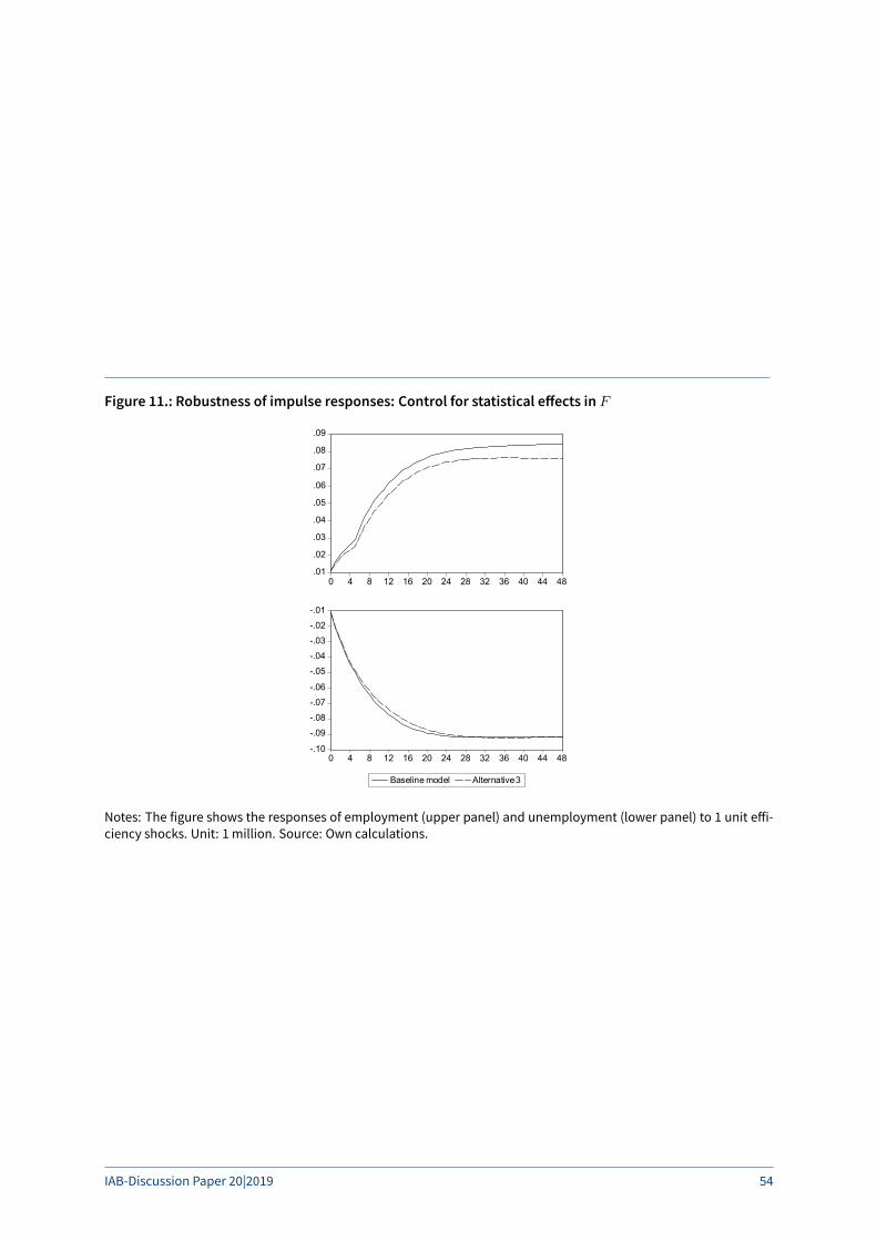
Figure 11.: Robustness of impulse responses: Control for statistical e�ects in F

.01

.02

.03

.04

.05

.06

.07

.08

.09

0 4 8 12 16 20 24 28 32 36 40 44 48

-.10

-.09-.08-.07-.06

-.05-.04-.03-.02-.01

0 4 8 12 16 20 24 28 32 36 40 44 48

Baseline model Alternative 3

Notes: The figure shows the responses of employment (upper panel) and unemployment (lower panel) to 1 unit e�i-ciency shocks. Unit: 1 million. Source: Own calculations.


Imprint

IAB-Discussion Paper 20|2019

Publication Date27 September 2019

PublisherInstitute for Employment Researchof the Federal Employment AgencyRegensburger Straße 10490478 NürnbergGermany

All rights reservedReproduction and distribution in any form – also in parts – requires the permission of IAB.

Downloadhttp://doku.iab.de/discussionpapers/2019/dp2019.pdf

All publications in the series “IAB-Discusssion Paper” can be downloaded fromhttps://www.iab.de/en/publikationen/discussionpaper.aspx

Websitewww.iab.de/en

Corresponding authorChristian HutterTelefon 0911 179-3057E-Mail [email protected]

which factors are behind germany's labour market upswing?

Documents