whirlpool: improving dynamic cache management with static … · 2016-02-10 · through case...
TRANSCRIPT
Whirlpool: Improving Dynamic Cache
Management with Static Data Classification
Anurag Mukkara Nathan Beckmann Daniel Sanchez
Computer Science and Artificial Intelligence Laboratory
Massachusetts Institute of Technology
{anuragm, beckmann, sanchez}@csail.mit.edu
Abstract
Cache hierarchies are increasingly non-uniform and difficult
to manage. Several techniques, such as scratchpads or reuse
hints, use static information about how programs access
data to manage the memory hierarchy. Static techniques are
effective on regular programs, but because they set fixed
policies, they are vulnerable to changes in program behavior
or available cache space. Instead, most systems rely on
dynamic caching policies that adapt to observed program
behavior. Unfortunately, dynamic policies spend significant
resources trying to learn how programs use memory, and yet
they often perform worse than a static policy.
We present Whirlpool, a novel approach that combines
static information with dynamic policies to reap the benefits
of each. Whirlpool statically classifies data into pools based
on how the program uses memory. Whirlpool then uses
dynamic policies to tune the cache to each pool. Hence, rather
than setting policies statically, Whirlpool uses static analysis
to guide dynamic policies. We present both an API that lets
programmers specify pools manually and a profiling tool that
discovers pools automatically in unmodified binaries.
We evaluate Whirlpool on a state-of-the-art NUCA cache.
Whirlpool significantly outperforms prior approaches: on
sequential programs, Whirlpool improves performance by up
to 38% and reduces data movement energy by up to 53%; on
parallel programs, Whirlpool improves performance by up to
67% and reduces data movement energy by up to 2.6×.
CCS Concepts
• Computer systems organization → Multicore architectures.
Keywords Non-uniform cache access (NUCA), Data move-
ment, Static analysis, Cache modeling.
Permission to make digital or hard copies of all or part of this work for personal orclassroom use is granted without fee provided that copies are not made or distributedfor profit or commercial advantage and that copies bear this notice and the full citationon the first page. Copyrights for components of this work owned by others than theauthor(s) must be honored. Abstracting with credit is permitted. To copy otherwise, orrepublish, to post on servers or to redistribute to lists, requires prior specific permissionand/or a fee. Request permissions from [email protected].
ASPLOS ’16, April 2–6, 2016, Atlanta, Georgia, USA.Copyright is held by the owner/author(s). Publication rights licensed to ACM.ACM 978-1-4503-4091-5/16/04. . . $15.00.http://dx.doi.org/10.1145/2872362.2872363
1. Introduction
Future systems will be limited by data movement, which
is orders of magnitude more expensive than basic compute
operations. For example, at 28 nm a 64-bit floating-point
multiply-add consumes 20 pJ, while sending 256 bits across
the chip costs 300 pJ, an on-chip access to a 1 MB cache
costs about 1 nJ, and an off-chip DRAM access costs 20-
50 nJ—1000× more energy than the multiply-add [21, 36, 59].
The trend towards lean, specialized cores means that, for
efficiency reasons, caches are increasingly distributed across
the chip and have non-uniform access latencies (NUCA [37]).
While distributed caches are more efficient, they are also
harder to manage. Their non-uniform latency and energy
means that data placement is critical to limit data movement.
But data placement is hard: applications need to fit their most
intensely-used data in nearby banks, while competing with
each other for scarce capacity. Data placement is a spatial
scheduling problem that, to solve well, requires accurate
information about how programs use memory.
Unfortunately, all the relevant information is not gener-
ally available: static analysis or profiling can reveal program
semantics (i.e., how a program uses memory), but not its
dynamic or input-dependent behavior; and dynamic policies
have difficulty efficiently recovering program semantics. To
see this in more detail, consider the extremes of static vs.
dynamic design. At one extreme, scratchpad-based systems
expose the distributed memories to software, relying on static
analysis to place data. Scratchpads work well on regular ac-
cess patterns, but cope poorly with irregular, input-dependent,
or rapidly changing patterns and varying resources in shared
systems [38, 41]. At the other extreme, cache-based systems
expose a flat address space that programs access through un-
differentiated loads and stores, relying on hardware-managed
caches to transparently retain the right data. Most memory
systems are cache-based, but recovering program semantics
from this limited interface is difficult and expensive. For ex-
ample, classic dynamic NUCA schemes migrate data towards
the requester in response to each access, which increases
data movement and requires expensive lookups [7, 9, 28]. As
memory systems become more complex, ignoring program
semantics becomes increasingly inefficient.
1
Prior work exploits static information in cache-based sys-
tems through prefetch [34], bypass [48], and cache prior-
ity [27] hints. Hints let software override dynamic policies
and control the cache, reaping the benefits of static informa-
tion when it is accurate. However, hints suffer from the same
problems as scratchpads: with uncertain or dynamic behavior,
hints are often inaccurate and hurt performance [41, 47].
The key idea of this paper is to combine static information
with dynamic policies to reap the benefits of each. Rather
than using static information to set fixed policies, we instead
use it to inform dynamic policies. The insight is that, while
uncertainty makes it hard to statically predict how data will
be used, it is often easy to accurately group data with similar
usage patterns. This approach lets dynamic policies make
better decisions at lower overhead.
We demonstrate this idea through Whirlpool, a classification-
based approach to improve data placement in multicores. In
Whirlpool, programs divide their data into a small number of
memory pools, e.g. one for each major data structure. We find
that for most programs, a few pools (three or four) suffice.
Hardware then monitors each pool dynamically and adapts
the memory system to keep the most valuable data near where
it is used. Unlike hints, pools do not encode static policies;
rather, they make it easy for hardware to find the right policies
dynamically. Whirlpool thus combines static program seman-
tics with dynamic policies, and robustly adapts to changes in
program behavior or available resources (Sec. 2).
Whirlpool has both software and hardware components
(Sec. 3). In software, Whirlpool provides a memory allocator
that groups semantically similar data and tags each page
with a pool id. In hardware, Whirlpool extends prior NUCA
techniques [9, 11] to monitor each pool and control its
placement. Whirlpool needs only a few pools, so it adds small
overheads. We first evaluate Whirlpool by manually applying
it to several SPEC CPU2006 and PBBS benchmarks. We show
that Whirlpool achieves significant performance gains, of up
to 38%, when managing a large NUCA cache, and reduces
data movement energy by up to 53%. Through case studies,
we also show that Whirlpool improves the performance of
parallel applications on a 16-core chip by up to 67% and
reduces data movement energy by up to 2.6×.
We then use the insights gained from manually porting
applications to design WhirlTool, a profiling tool that auto-
matically discovers pools in unmodified binaries (Sec. 4). We
evaluate WhirlTool on a comprehensive set of benchmarks
and program mixes, and find that it works as well or better
than our careful manual classification.
In summary, Whirlpool gives a promising way to combine
static program semantics and dynamic policies to reduce data
movement.
2. Motivation and Background
In this section, we motivate Whirlpool’s hybrid, static-
dynamic design and discuss related work.
2.1 How static classification reduces data movement
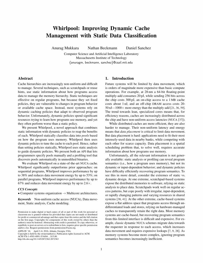
Consider the multicore shown in Fig. 1. This chip has a
NUCA cache of twenty-five 512 KB banks shared by four
surrounding cores, similar to the Oracle SPARC M7 [3]
(see Appendix A for detailed methodology). We consider
the benchmark dt (Delaunay triangulation) from the PBBS
suite [60], running in the leftmost core. Our goal is to use this
distributed cache capacity as efficiently as possible by placing
dt’s most intensely used data near where dt is running.
dt
Figure 1: Multicore chip with a
distributed last-level cache.
0
1
2
3
4
5
6
Wo
rkin
g s
et
(MB
)
0
5
10
15
20
25
Acce
sse
s p
er
K-in
str
.
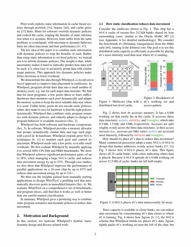
Figure 2: Breakdown of
dt’s working set and
access pattern.
Fig. 2 shows how dt accesses memory. It has a 6 MB
working set that easily fits in the cache. It accesses three
data structures: points, vertices, and triangles, which take
0.5 MB, 1.5 MB, and 4 MB, respectively. Accesses are split
roughly evenly across the three data structures, so their access
intensity (i.e., accesses per MB) varies: points are accessed
most intensely, followed by vertices and triangles.
How should we place dt’s data to reduce data movement?
Many commercial processors adopt a static NUCA (S-NUCA)
design that hashes addresses evenly across banks [37, 53].
Fig. 3 shows how S-NUCA places dt’s data. This figure
shows all 25 cache banks, with colors indicating where data
is placed. Because S-NUCA spreads dt’s 6 MB working set
across 12.5 MB of cache, banks are left half-empty.
dt
Triangles
Vertices
Points
Figure 3: S-NUCA places dt’s data unnecessarily far away.
Since capacity is available in closer banks, we can reduce
data movement by concentrating dt’s data closer to where
dt is running. Fig. 4 shows how Jigsaw [9, 11], the NUCA
scheme that Whirlpool builds on, places dt’s data. Jigsaw
tightly packs dt’s working set near the left of the chip, but
2
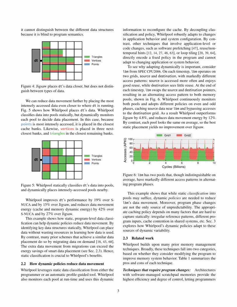
it cannot distinguish between the different data structures
because it is blind to program semantics.
dt
Triangles
Vertices
Points
Figure 4: Jigsaw places dt’s data closer, but does not distin-
guish between types of data.
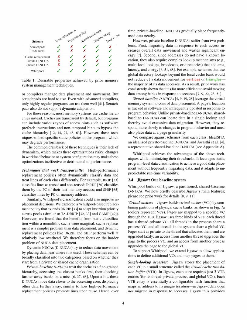
We can reduce data movement further by placing the most
intensely accessed data even closer to where dt is running.
Fig. 5 shows how Whirlpool places dt’s data. Whirlpool
classifies data into pools statically, but dynamically monitors
each pool to decide data placement. In this case, because
points is most intensely accessed, it is placed in the closest
cache banks. Likewise, vertices is placed in three next-
closest banks, and triangles in the closest remaining banks.
dt
Triangles
Vertices
Points
Figure 5: Whirlpool statically classifies dt’s data into pools,
and dynamically places intensely-accessed pools nearby.
Whirlpool improves dt’s performance by 19% over S-
NUCA and by 15% over Jigsaw, and reduces data movement
energy (cache and memory dynamic energy) by 42% over
S-NUCA and by 27% over Jigsaw.
This example shows how static, program-level data classi-
fication can help dynamic policies reduce data movement. By
identifying key data structures statically, Whirlpool can place
data without wasting resources in learning how data is used.
By contrast, many prior schemes that achieve a similar data
placement do so by migrating data on demand [18, 43, 68].
The extra data movement from migrations can exceed the
energy savings of smart data placement (see Sec. 2.3). Hence,
static classification is crucial to Whirlpool’s benefits.
2.2 How dynamic policies reduce data movement
Whirlpool leverages static data classification from either the
programmer or an automatic profile-guided tool. Whirlpool
also monitors each pool at run-time and uses this dynamic
information to reconfigure the cache. By decoupling clas-
sification and policy, Whirlpool robustly adapts to changes
in application behavior and system configuration. By con-
trast, other techniques that involve application-level or
code changes, such as software prefetching [47], reuse/non-
temporal hints [12, 14, 27, 48, 63], or loop tiling [20, 39, 64],
directly encode a fixed policy in the program and cannot
adapt to changing application or system behavior.
To see why adapting dynamically is important, consider
lbm from SPEC CPU2006. On each timestep, lbm operates on
two grids, source and destination, with markedly different
access patterns: source is accessed more often and enjoys
good reuse, while destination sees little reuse. At the end of
each timestep, lbm swaps the source and destination pointers,
resulting in an alternating access pattern to both memory
pools, shown in Fig. 6. Whirlpool continuously monitors
both pools and adopts different policies on even and odd
phases, caching source data near lbm and bypassing accesses
to the destination grid. As a result Whirlpool outperforms
Jigsaw by 4.8%, and reduces data movement energy by 12%.
By contrast, each pool looks the same on average, so the best
static placement yields no improvement over Jigsaw.
0 2 4 6 8 10
Cycles (Billions)
0
20
40
60
80
100
Acce
sse
s (
AP
KI)
Grid1 Grid2
Figure 6: lbm has two pools that, though indistinguishable on
average, have markedly different access patterns in alternat-
ing program phases.
This example shows that while static classification into
pools may suffice, dynamic policies are needed to reduce
lbm’s data movement. Moreover, program phase changes
are not the only source of unpredictability. The appropri-
ate caching policy depends on many factors that are hard to
capture statically: irregular reference patterns, different pro-
gram inputs, cache contention in shared systems, etc. Sec. 3
explores how Whirlpool’s dynamic policies adapt to these
sources of dynamic variability.
2.3 Related work
Whirlpool builds upon many prior memory management
techniques. Broadly, these techniques fall into two categories,
based on whether they consider modifying the program to
improve memory system behavior. Table 1 summarizes the
pros and cons of each technique.
Techniques that require program changes: Architectures
with software-managed scratchpad memories provide the
highest efficiency and degree of control, letting programmers
3
Scheme Staticinform
ation
Dynamicpolic
y
Spatial placement
Single-lookup
Easyto
use
Scratchpads ✓ ✗ ✓ ✓ ✗
Code hints ✓ ✗ ✗ ✓ ✓
Cache replacement ✗ ✓ ✗ ✓ ✓
Private D-NUCA ✗ ✓ ✓ ✗ ✓
Shared D-NUCA ✗ ✓ ✓ ✓ ✓
Whirlpool ✓ ✓ ✓ ✓ ✓
Table 1: Desirable properties achieved by prior memory
system management techniques.
or compilers manage data placement and movement. But
scratchpads are hard to use. Even with advanced compilers,
only highly regular programs can use them well [41]. Scratch-
pads also do not support dynamic adaptation.
For these reasons, most memory systems use cache hierar-
chies instead. Caches are transparent by default, but programs
can include various types of access hints such as software
prefetch instructions and non-temporal hints to bypass the
cache hierarchy [12, 14, 27, 48, 63]. However, these tech-
niques embed specific static policies in the program, which
may degrade performance.
The common drawback of these techniques is their lack of
dynamism, which makes these optimizations risky: changes
in workload behavior or system configuration may make these
optimizations ineffective or detrimental to performance.
Techniques that work transparently: High-performance
replacement policies often dynamically classify data and
treat lines of each class differently. For example, RRIP [33]
classifies lines as reused and non-reused; IbRDP [50] classifies
them by the PC of their last memory access; and SHiP [65]
classifies lines by PC or memory address.
Similarly, Whirlpool’s classification could also improve re-
placement decisions. We explored a Whirlpool-based replace-
ment policy that extends DRRIP [33] to adapt insertion priority
across pools (similar to TA-DRRIP [32, 33] and CAMP [49]).
However, we found that the benefits from static classifica-
tion within a monolithic cache were marginal: cache replace-
ment is a simpler problem than data placement, and dynamic
replacement policies like DRRIP and SHiP perform well at
relatively low overhead. We therefore focus on the harder
problem of NUCA data placement.
Dynamic NUCAs (D-NUCAs) try to reduce data movement
by placing data near where it is used. These schemes can be
broadly classified into two categories based on whether they
start from a private or shared cache organization.
Private-baseline D-NUCAs treat the cache as a fine-grained
hierarchy, accessing the closest banks first, then checking
farther-away banks on a miss [6, 37, 68]. Upon a hit, these
D-NUCAs move data closer to the accessing core, displacing
other data further away, similar to how high-performance
replacement policies promote lines upon reuse. Hence, over
time, private-baseline D-NUCAs gradually place frequently-
used data nearby.
However, private-baseline D-NUCAs suffer from two prob-
lems. First, migrating data in response to each access in-
creases overall data movement and wastes significant en-
ergy [7]. Second, since addresses do not have a known lo-
cation, they also require complex lookup mechanisms (e.g.,
multi-level lookups, broadcasts, or directories) that add area,
latency, and energy [6, 51, 68]. For example, schemes that use
global directory lookups beyond the local cache bank would
not reduce dt’s data movement for vertices or triangles—
the majority of its data accesses. As a result, prior work has
consistently shown that it is far more efficient to avoid moving
data among banks in response to accesses [7, 9, 22, 28, 51].
Shared-baseline D-NUCAs [4, 9, 19, 28] leverage the virtual
memory system to control data placement. A page’s location
is tracked in software and infrequently updated in response to
program behavior. Unlike private-baseline D-NUCAs, shared-
baseline D-NUCAs can locate data in a single lookup and
thereby avoid excessive data migration. However, they re-
spond more slowly to changes in program behavior and must
also place data at a page granularity.
We compare against schemes from each class: IdealSPD,
an idealized private-baseline D-NUCA, and Awasthi et al. [4],
a representative shared-baseline D-NUCA (see Appendix A).
Whirlpool achieves the advantages of the above tech-
niques while minimizing their drawbacks. It leverages static,
program-level data classification to achieve a good data place-
ment without frequently migrating data, and it adapts to un-
predictable run-time variability.
2.4 Jigsaw: Our baseline system
Whirlpool builds on Jigsaw, a partitioned, shared-baseline
D-NUCA. We now briefly describe Jigsaw’s main features;
please see prior work for details [8, 9, 11].
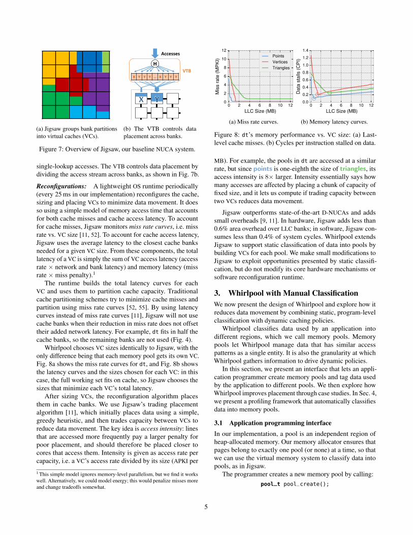
Virtual caches: Jigsaw builds virtual caches (VCs) by com-
bining partitions of physical cache banks, as shown in Fig. 7a
(colors represent VCs). Pages are mapped to a specific VC
through the TLB. Jigsaw uses three kinds of VCs: each thread
has a thread-private VC; all threads in the process share a
process VC; and all threads in the system share a global VC.
Pages start as private to the thread that allocates them, and are
upgraded lazily: an access from another thread upgrades the
page to the process VC, and an access from another process
upgrades the page to the global VC.
To support Whirlpool, we extend Jigsaw to allow applica-
tions to define additional VCs and map pages to them.
Single-lookup accesses: Jigsaw stores the placement of
each VC in a small structure called the virtual cache transla-
tion buffer (VTB). In Jigsaw, each core requires just 3 VTB
entries (for its thread-private, process, and global VCs). Each
VTB entry is essentially a configurable hash function that
maps an address to its unique location—in Jigsaw, data does
not migrate in response to accesses. Jigsaw thus provides
4
(a) Jigsaw groups bank partitions
into virtual caches (VCs).
Accesses
H
VTB
X Y Y Y … X Y Y Y
(b) The VTB controls data
placement across banks.
Figure 7: Overview of Jigsaw, our baseline NUCA system.
single-lookup accesses. The VTB controls data placement by
dividing the access stream across banks, as shown in Fig. 7b.
Reconfigurations: A lightweight OS runtime periodically
(every 25 ms in our implementation) reconfigures the cache,
sizing and placing VCs to minimize data movement. It does
so using a simple model of memory access time that accounts
for both cache misses and cache access latency. To account
for cache misses, Jigsaw monitors miss rate curves, i.e. miss
rate vs. VC size [11, 52]. To account for cache access latency,
Jigsaw uses the average latency to the closest cache banks
needed for a given VC size. From these components, the total
latency of a VC is simply the sum of VC access latency (access
rate × network and bank latency) and memory latency (miss
rate × miss penalty).1
The runtime builds the total latency curves for each
VC and uses them to partition cache capacity. Traditional
cache partitioning schemes try to minimize cache misses and
partition using miss rate curves [52, 55]. By using latency
curves instead of miss rate curves [11], Jigsaw will not use
cache banks when their reduction in miss rate does not offset
their added network latency. For example, dt fits in half the
cache banks, so the remaining banks are not used (Fig. 4).
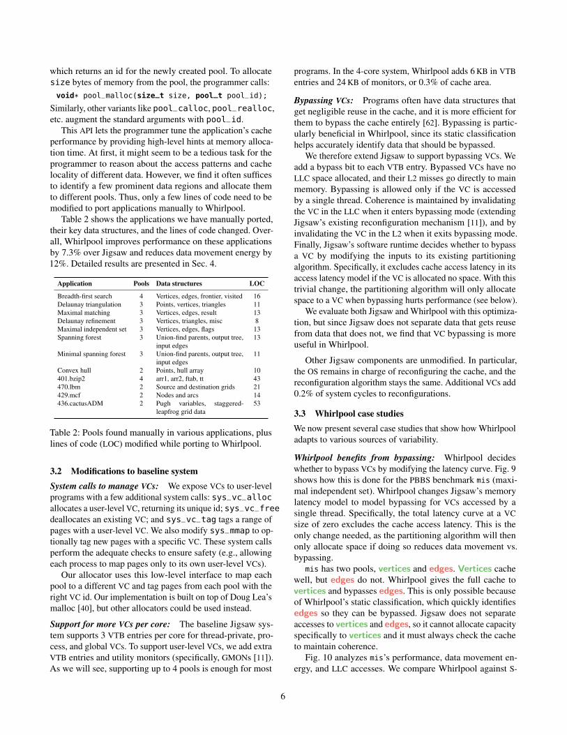
Whirlpool chooses VC sizes identically to Jigsaw, with the
only difference being that each memory pool gets its own VC.
Fig. 8a shows the miss rate curves for dt, and Fig. 8b shows
the latency curves and the sizes chosen for each VC: in this
case, the full working set fits on cache, so Jigsaw chooses the
sizes that minimize each VC’s total latency.
After sizing VCs, the reconfiguration algorithm places
them in cache banks. We use Jigsaw’s trading placement
algorithm [11], which initially places data using a simple,
greedy heuristic, and then trades capacity between VCs to
reduce data movement. The key idea is access intensity: lines
that are accessed more frequently pay a larger penalty for
poor placement, and should therefore be placed closer to
cores that access them. Intensity is given as access rate per
capacity, i.e. a VC’s access rate divided by its size (APKI per
1 This simple model ignores memory-level parallelism, but we find it works
well. Alternatively, we could model energy; this would penalize misses more
and change tradeoffs somewhat.
0 2 4 6 8 10 12
LLC Size (MB)
0
2
4
6
8
10
12
Mis
s r
ate
(M
PK
I)
Points
Vertices
Triangles
(a) Miss rate curves.
0 2 4 6 8 10 12
LLC Size (MB)
0.0
0.2
0.4
0.6
0.8
1.0
1.2
1.4
Data
sta
lls (
CP
I)
(b) Memory latency curves.
Figure 8: dt’s memory performance vs. VC size: (a) Last-
level cache misses. (b) Cycles per instruction stalled on data.
MB). For example, the pools in dt are accessed at a similar
rate, but since points is one-eighth the size of triangles, its
access intensity is 8× larger. Intensity essentially says how
many accesses are affected by placing a chunk of capacity of
fixed size, and it lets us compute if trading capacity between
two VCs reduces data movement.
Jigsaw outperforms state-of-the-art D-NUCAs and adds
small overheads [9, 11]. In hardware, Jigsaw adds less than
0.6% area overhead over LLC banks; in software, Jigsaw con-
sumes less than 0.4% of system cycles. Whirlpool extends
Jigsaw to support static classification of data into pools by
building VCs for each pool. We make small modifications to
Jigsaw to exploit opportunities presented by static classifi-
cation, but do not modify its core hardware mechanisms or
software reconfiguration runtime.
3. Whirlpool with Manual Classification
We now present the design of Whirlpool and explore how it
reduces data movement by combining static, program-level
classification with dynamic caching policies.
Whirlpool classifies data used by an application into
different regions, which we call memory pools. Memory
pools let Whirlpool manage data that has similar access
patterns as a single entity. It is also the granularity at which
Whirlpool gathers information to drive dynamic policies.
In this section, we present an interface that lets an appli-
cation programmer create memory pools and tag data used
by the application to different pools. We then explore how
Whirlpool improves placement through case studies. In Sec. 4,
we present a profiling framework that automatically classifies
data into memory pools.
3.1 Application programming interface
In our implementation, a pool is an independent region of
heap-allocated memory. Our memory allocator ensures that
pages belong to exactly one pool (or none) at a time, so that
we can use the virtual memory system to classify data into
pools, as in Jigsaw.
The programmer creates a new memory pool by calling:
pool_t pool_create();
5
which returns an id for the newly created pool. To allocate
size bytes of memory from the pool, the programmer calls:
void* pool_malloc(size_t size, pool_t pool_id);
Similarly, other variants like pool_calloc, pool_realloc,
etc. augment the standard arguments with pool_id.
This API lets the programmer tune the application’s cache
performance by providing high-level hints at memory alloca-
tion time. At first, it might seem to be a tedious task for the
programmer to reason about the access patterns and cache
locality of different data. However, we find it often suffices
to identify a few prominent data regions and allocate them
to different pools. Thus, only a few lines of code need to be
modified to port applications manually to Whirlpool.
Table 2 shows the applications we have manually ported,
their key data structures, and the lines of code changed. Over-
all, Whirlpool improves performance on these applications
by 7.3% over Jigsaw and reduces data movement energy by
12%. Detailed results are presented in Sec. 4.
Application Pools Data structures LOC
Breadth-first search 4 Vertices, edges, frontier, visited 16
Delaunay triangulation 3 Points, vertices, triangles 11
Maximal matching 3 Vertices, edges, result 13
Delaunay refinement 3 Vertices, triangles, misc 8
Maximal independent set 3 Vertices, edges, flags 13
Spanning forest 3 Union-find parents, output tree,
input edges
13
Minimal spanning forest 3 Union-find parents, output tree,
input edges
11
Convex hull 2 Points, hull array 10
401.bzip2 4 arr1, arr2, ftab, tt 43
470.lbm 2 Source and destination grids 21
429.mcf 2 Nodes and arcs 14
436.cactusADM 2 Pugh variables, staggered-
leapfrog grid data
53
Table 2: Pools found manually in various applications, plus
lines of code (LOC) modified while porting to Whirlpool.
3.2 Modifications to baseline system
System calls to manage VCs: We expose VCs to user-level
programs with a few additional system calls: sys_vc_alloc
allocates a user-level VC, returning its unique id; sys_vc_free
deallocates an existing VC; and sys_vc_tag tags a range of
pages with a user-level VC. We also modify sys_mmap to op-
tionally tag new pages with a specific VC. These system calls
perform the adequate checks to ensure safety (e.g., allowing
each process to map pages only to its own user-level VCs).
Our allocator uses this low-level interface to map each
pool to a different VC and tag pages from each pool with the
right VC id. Our implementation is built on top of Doug Lea’s
malloc [40], but other allocators could be used instead.
Support for more VCs per core: The baseline Jigsaw sys-
tem supports 3 VTB entries per core for thread-private, pro-
cess, and global VCs. To support user-level VCs, we add extra
VTB entries and utility monitors (specifically, GMONs [11]).
As we will see, supporting up to 4 pools is enough for most
programs. In the 4-core system, Whirlpool adds 6 KB in VTB
entries and 24 KB of monitors, or 0.3% of cache area.
Bypassing VCs: Programs often have data structures that
get negligible reuse in the cache, and it is more efficient for
them to bypass the cache entirely [62]. Bypassing is partic-
ularly beneficial in Whirlpool, since its static classification
helps accurately identify data that should be bypassed.
We therefore extend Jigsaw to support bypassing VCs. We
add a bypass bit to each VTB entry. Bypassed VCs have no
LLC space allocated, and their L2 misses go directly to main
memory. Bypassing is allowed only if the VC is accessed
by a single thread. Coherence is maintained by invalidating
the VC in the LLC when it enters bypassing mode (extending
Jigsaw’s existing reconfiguration mechanism [11]), and by
invalidating the VC in the L2 when it exits bypassing mode.
Finally, Jigsaw’s software runtime decides whether to bypass
a VC by modifying the inputs to its existing partitioning
algorithm. Specifically, it excludes cache access latency in its
access latency model if the VC is allocated no space. With this
trivial change, the partitioning algorithm will only allocate
space to a VC when bypassing hurts performance (see below).
We evaluate both Jigsaw and Whirlpool with this optimiza-
tion, but since Jigsaw does not separate data that gets reuse
from data that does not, we find that VC bypassing is more
useful in Whirlpool.
Other Jigsaw components are unmodified. In particular,
the OS remains in charge of reconfiguring the cache, and the
reconfiguration algorithm stays the same. Additional VCs add
0.2% of system cycles to reconfigurations.
3.3 Whirlpool case studies
We now present several case studies that show how Whirlpool
adapts to various sources of variability.
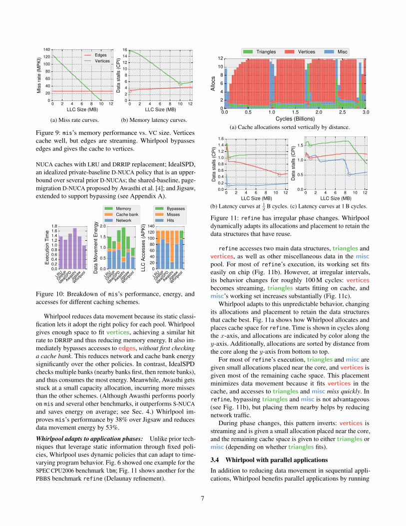
Whirlpool benefits from bypassing: Whirlpool decides
whether to bypass VCs by modifying the latency curve. Fig. 9
shows how this is done for the PBBS benchmark mis (maxi-
mal independent set). Whirlpool changes Jigsaw’s memory
latency model to model bypassing for VCs accessed by a
single thread. Specifically, the total latency curve at a VC
size of zero excludes the cache access latency. This is the
only change needed, as the partitioning algorithm will then
only allocate space if doing so reduces data movement vs.
bypassing.
mis has two pools, vertices and edges. Vertices cache
well, but edges do not. Whirlpool gives the full cache to
vertices and bypasses edges. This is only possible because
of Whirlpool’s static classification, which quickly identifies
edges so they can be bypassed. Jigsaw does not separate
accesses to vertices and edges, so it cannot allocate capacity
specifically to vertices and it must always check the cache
to maintain coherence.
Fig. 10 analyzes mis’s performance, data movement en-
ergy, and LLC accesses. We compare Whirlpool against S-
6
0 2 4 6 8 10 12
LLC Size (MB)
0
20
40
60
80
100
120
140
Mis
s r
ate
(M
PK
I)
Edges
Vertices
(a) Miss rate curves.
0 2 4 6 8 10 12
LLC Size (MB)
0
2
4
6
8
10
12
14
16
Data
sta
lls (
CP
I)(b) Memory latency curves.
Figure 9: mis’s memory performance vs. VC size. Vertices
cache well, but edges are streaming. Whirlpool bypasses
edges and gives the cache to vertices.
NUCA caches with LRU and DRRIP replacement; IdealSPD,
an idealized private-baseline D-NUCA policy that is an upper-
bound over several prior D-NUCAs; the shared-baseline, page-
migration D-NUCA proposed by Awasthi et al. [4]; and Jigsaw,
extended to support bypassing (see Appendix A).
LRU
DRRIP
Idea
lSPD
Awas
thi
Jigs
aw
Whirlp
ool
0.00.20.40.60.81.01.21.41.61.8
Execution T
ime
LRU
DRRIP
Idea
lSPD
Awas
thi
Jigs
aw
Whirlp
ool
0.0
0.5
1.0
1.5
2.0
Data
Movem
ent E
nerg
y
Memory
Cache bank
Network
LRU
DRRIP
Idea
lSPD
Awas
thi
Jigs
aw
Whirlp
ool
0
20
40
60
80
100
120
140
LLC
Accesses (
AP
KI)
Bypasses
Misses
Hits
Figure 10: Breakdown of mis’s performance, energy, and
accesses for different caching schemes.
Whirlpool reduces data movement because its static classi-
fication lets it adopt the right policy for each pool. Whirlpool
gives enough space to fit vertices, achieving a similar hit
rate to DRRIP and thus reducing memory energy. It also im-
mediately bypasses accesses to edges, without first checking
a cache bank. This reduces network and cache bank energy
significantly over the other policies. In contrast, IdealSPD
checks multiple banks (nearby banks first, then remote banks),
and thus consumes the most energy. Meanwhile, Awasthi gets
stuck at a small capacity allocation, incurring more misses
than the other schemes. (Although Awasthi performs poorly
on mis and several other benchmarks, it outperforms S-NUCA
and saves energy on average; see Sec. 4.) Whirlpool im-
proves mis’s performance by 38% over Jigsaw and reduces
data movement energy by 53%.
Whirlpool adapts to application phases: Unlike prior tech-
niques that leverage static information through fixed poli-
cies, Whirlpool uses dynamic policies that can adapt to time-
varying program behavior. Fig. 6 showed one example for the
SPEC CPU2006 benchmark lbm; Fig. 11 shows another for the
PBBS benchmark refine (Delaunay refinement).
0.0 0.5 1.0 1.5 2.0 2.5 3.0
Cycles (Billions)
0
2
4
6
8
10
12
Allo
cs
Triangles Vertices Misc
(a) Cache allocations sorted vertically by distance.
0 2 4 6 8 10 12
LLC Size (MB)
0.0
0.2
0.4
0.6
0.8
1.0
1.2
1.4
1.6
Data
sta
lls (
CP
I)
(b) Latency curves at 1
2B cycles.
0 2 4 6 8 10 12
LLC Size (MB)
0.0
0.5
1.0
1.5
Data
sta
lls (
CP
I)
(c) Latency curves at 1 B cycles.
Figure 11: refine has irregular phase changes. Whirlpool
dynamically adapts its allocations and placement to retain the
data structures that have reuse.
refine accesses two main data structures, triangles and
vertices, as well as other miscellaneous data in the misc
pool. For most of refine’s execution, its working set fits
easily on chip (Fig. 11b). However, at irregular intervals,
its behavior changes for roughly 100 M cycles: vertices
becomes streaming, triangles starts fitting on cache, and
misc’s working set increases substantially (Fig. 11c).
Whirlpool adapts to this unpredictable behavior, changing
its allocations and placement to retain the data structures
that cache best. Fig. 11a shows how Whirlpool allocates and
places cache space for refine. Time is shown in cycles along
the x-axis, and allocations are indicated by color along the
y-axis. Additionally, allocations are sorted by distance from
the core along the y-axis from bottom to top.
For most of refine’s execution, triangles and misc are
given small allocations placed near the core, and vertices is
given most of the remaining cache space. This placement
minimizes data movement because it fits vertices in the
cache, and accesses to triangles and misc miss quickly. In
refine, bypassing triangles and misc is not advantageous
(see Fig. 11b), but placing them nearby helps by reducing
network traffic.
During phase changes, this pattern inverts: vertices is
streaming and is given a small allocation placed near the core,
and the remaining cache space is given to either triangles or
misc (depending on whether triangles fits).
3.4 Whirlpool with parallel applications
In addition to reducing data movement in sequential appli-
cations, Whirlpool benefits parallel applications by running
7
tasks close to their data. Whirlpool makes small changes to
task-parallel runtimes, letting it rapidly benefit many applica-
tions with minimal programmer burden.
Conventional work-stealing: Work-stealing [13] is the
most widely-used scheduling technique for task-parallel
programs. Each thread has a queue of ready tasks, to which
it enqueues and dequeues work. When a thread runs out of
work, it tries to steal tasks from a randomly-selected thread’s
queue. Work-stealing makes task enqueues and dequeues
cheap and achieves good load balance, but, over time, each
core ends up accessing data used by many tasks, hurting
locality. Since work-stealing causes poor reference locality,
D-NUCAs alone cannot achieve a good data placement [11].
For example, as shown in Fig. 13, Jigsaw performs the same
as S-NUCA because most data is accessed from multiple cores
and mapped to the single process-level VC.
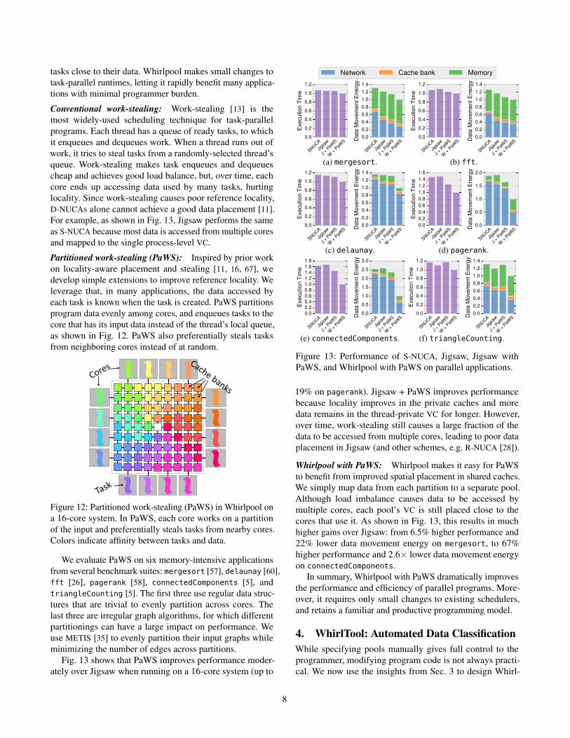
Partitioned work-stealing (PaWS): Inspired by prior work
on locality-aware placement and stealing [11, 16, 67], we
develop simple extensions to improve reference locality. We
leverage that, in many applications, the data accessed by
each task is known when the task is created. PaWS partitions
program data evenly among cores, and enqueues tasks to the
core that has its input data instead of the thread’s local queue,
as shown in Fig. 12. PaWS also preferentially steals tasks
from neighboring cores instead of at random.
Figure 12: Partitioned work-stealing (PaWS) in Whirlpool on
a 16-core system. In PaWS, each core works on a partition
of the input and preferentially steals tasks from nearby cores.
Colors indicate affinity between tasks and data.
We evaluate PaWS on six memory-intensive applications
from several benchmark suites: mergesort [57], delaunay [60],
fft [26], pagerank [58], connectedComponents [5], and
triangleCounting [5]. The first three use regular data struc-
tures that are trivial to evenly partition across cores. The
last three are irregular graph algorithms, for which different
partitionings can have a large impact on performance. We
use METIS [35] to evenly partition their input graphs while
minimizing the number of edges across partitions.
Fig. 13 shows that PaWS improves performance moder-
ately over Jigsaw when running on a 16-core system (up to
Network Cache bank Memory
SNUCA
Jigs
aw
J +
PaWS
W +
PaW
S0.0
0.2
0.4
0.6
0.8
1.0
1.2
Execution T
ime
SNUCA
Jigs
aw
J +
PaWS
W +
PaW
S0.0
0.2
0.4
0.6
0.8
1.0
1.2
1.4
Data
Movem
ent E
nerg
y
(a) mergesort.
SNUCA
Jigs
aw
J +
PaWS
W +
PaW
S0.0
0.2
0.4
0.6
0.8
1.0
1.2
Execution T
ime
SNUCA
Jigs
aw
J +
PaWS
W +
PaW
S0.0
0.2
0.4
0.6
0.8
1.0
1.2
1.4
Data
Movem
ent E
nerg
y
(b) fft.
SNUCA
Jigs
aw
J +
PaWS
W +
PaW
S0.0
0.2
0.4
0.6
0.8
1.0
1.2
Execution T
ime
SNUCA
Jigs
aw
J +
PaWS
W +
PaW
S0.0
0.2
0.4
0.6
0.8
1.0
1.2
1.4
Data
Movem
ent E
nerg
y
(c) delaunay.
SNUCA
Jigs
aw
J +
PaWS
W +
PaW
S0.0
0.2
0.4
0.6
0.8
1.0
1.2
1.4
1.6
Execution T
ime
SNUCA
Jigs
aw
J +
PaWS
W +
PaW
S0.0
0.5
1.0
1.5
2.0
Data
Movem
ent E
nerg
y
(d) pagerank.
SNUCA
Jigs
aw
J +
PaWS
W +
PaW
S0.00.20.40.60.81.01.21.41.61.8
Execution T
ime
SNUCA
Jigs
aw
J +
PaWS
W +
PaW
S0.0
0.5
1.0
1.5
2.0
2.5
3.0
Data
Movem
ent E
nerg
y
(e) connectedComponents.
SNUCA
Jigs
aw
J +
PaWS
W +
PaW
S0.0
0.2
0.4
0.6
0.8
1.0
1.2
Execution T
ime
SNUCA
Jigs
aw
J +
PaWS
W +
PaW
S0.0
0.2
0.4
0.6
0.8
1.0
1.2
1.4
Data
Movem
ent E
nerg
y
(f) triangleCounting.
Figure 13: Performance of S-NUCA, Jigsaw, Jigsaw with
PaWS, and Whirlpool with PaWS on parallel applications.
19% on pagerank). Jigsaw + PaWS improves performance
because locality improves in the private caches and more
data remains in the thread-private VC for longer. However,
over time, work-stealing still causes a large fraction of the
data to be accessed from multiple cores, leading to poor data
placement in Jigsaw (and other schemes, e.g. R-NUCA [28]).
Whirlpool with PaWS: Whirlpool makes it easy for PaWS
to benefit from improved spatial placement in shared caches.
We simply map data from each partition to a separate pool.
Although load imbalance causes data to be accessed by
multiple cores, each pool’s VC is still placed close to the
cores that use it. As shown in Fig. 13, this results in much
higher gains over Jigsaw: from 6.5% higher performance and
22% lower data movement energy on mergesort, to 67%
higher performance and 2.6× lower data movement energy
on connectedComponents.
In summary, Whirlpool with PaWS dramatically improves
the performance and efficiency of parallel programs. More-
over, it requires only small changes to existing schedulers,
and retains a familiar and productive programming model.
4. WhirlTool: Automated Data Classification
While specifying pools manually gives full control to the
programmer, modifying program code is not always practi-
cal. We now use the insights from Sec. 3 to design Whirl-
8
Tool, a profile-guided tool that automatically classifies data
into pools. WhirlTool works on unmodified binaries, often
matches and sometimes outperforms our manual classifica-
tion, and introduces small overheads. WhirlTool is publicly
available at http://people.csail.mit.edu/sanchez.
WhirlTool
Analyzer
Whirlpool
Allocator
WhirlTool
RuntimeCallpoint-to-
pool map
Per-callpoint
miss curves
WhirlTool
Profiler
malloc()
pool_malloc()
Application
Figure 14: WhirlTool overview.
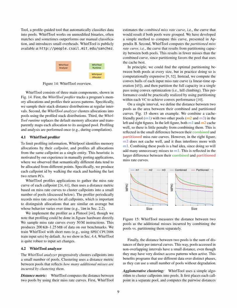
WhirlTool consists of three main components, shown in
Fig. 14. First, the WhirlTool profiler tracks a program’s mem-
ory allocations and profiles their access patterns. Specifically,
we sample their stack distance distributions at regular inter-
vals. Second, the WhirlTool analyzer clusters allocations into
pools using the profiled stack distributions. Third, the Whirl-
Tool runtime replaces the default memory allocator and trans-
parently maps each allocation to its assigned pool. Profiling
and analysis are performed once (e.g., during compilation).
4.1 WhirlTool profiler
To limit profiling information, Whirlpool identifies memory
allocations by their callpoint, and profiles all allocations
from the same callpoint as a single entity. This heuristic is
motivated by our experience in manually porting applications,
where we observed that semantically different data tend to
be allocated from different points. Specifically, we produce
each callpoint id by walking the stack and hashing the last
two return PCs.
WhirlTool profiles applications to gather the miss rate
curve of each callpoint [24, 61], then uses a distance metric
based on miss rate curves to cluster callpoints into a small
number of pools (discussed below). The profiler periodically
records miss rate curves for all callpoints, which is important
to distinguish allocations that are similar on average but
whose behavior varies over time (e.g., lbm in Sec. 2.2).
We implement the profiler as a Pintool [44], though we
note that profiling could be done in Jigsaw hardware directly.
We sample miss rate curves every 50 M instructions. This
produces 200 KB–1.25 MB of data on our benchmarks. We
train WhirlTool with short runs (e.g., using SPEC CPU2006
train input sets) by default. As we show in Sec. 4.4, WhirlTool
is quite robust to input set changes.
4.2 WhirlTool analyzer
The WhirlTool analyzer progressively clusters callpoints into
a small number of pools. Clustering uses a distance metric
between pools that reflects how many additional misses are
incurred by clustering them.
Distance metric: WhirlTool computes the distance between
two pools by using their miss rate curves. First, WhirlTool
estimates the combined miss rate curve, i.e., the curve that
would result if both pools were grouped. We have developed
a simple method to compute this curve, presented in Ap-
pendix B. Second, WhirlTool computes the partitioned miss
rate curve, i.e., the curve that results from partitioning capac-
ity between both pools. This results in fewer misses than the
combined curve, since partitioning favors the pool that uses
the cache best.
In principle, we could find the optimal partitioning be-
tween both pools at every size, but in practice doing so is
computationally expensive [9, 52]. Instead, we compute the
convex hulls of each input miss rate curve (a linear-time op-
eration [45]), and then partition the full capacity in a single
pass using convex optimization (i.e., hill climbing). This per-
formance could be practically realized by using partitioning
within each VC to achieve convex performance [10].
On a single interval, we define the distance between two
pools as the area between their combined and partitioned
curves. Fig. 15 shows an example. We combine a cache-
friendly pool (m1) with two other pools (m2 and m3) in the
left and right figures. In the left figure, both m1 and m2 cache
well, so there is little penalty from combining them. This is
reflected in the small difference between their combined and
partitioned miss rate curves. However, in the right figure,
m3 does not cache well, and it thus interferes more with
m1. Combining these pools is a bad idea, since doing so will
add many unnecessary misses to m1. This is reflected in the
larger difference between their combined and partitioned
miss rate curves.
Size
MP
KI
Size
MP
KI
m1 m2 m3 Combined Partitioned
Figure 15: WhirlTool measures the distance between two
pools as the additional misses incurred by combining the
pools vs. partitioning them separately.
Finally, the distance between two pools is the sum of dis-
tances of their per-interval curves. This way, pools accessed in
non-overlapping intervals have a small distance, even though
they may have very distinct access patterns when active. This
benefits programs that use different data over distinct phases,
as they can use a small number of pools without degradation.
Agglomerative clustering: WhirlTool uses a simple algo-
rithm to cluster callpoints into pools. It first places each call-
point in a separate pool, and computes the pairwise distances
9
-2
0
2
4
6
8
10
12
14
16
Sp
ee
du
p v
s J
igsa
w (
%)
bzi
p2
gcc
mcf
milc
zeus
cact
us
lesl
ie
sople
x
gem
s
libqntm lbm
om
net
ast
ar
sphin
x3
xala
nc
BFS
MIS
MS
T
SA
ST
dela
unay
dic
t
hull
isort
matc
hin
gneig
hbors ray
refin
e
rem
Dups
setC
ove
r
sort
38 38 38
2 pools 3 pools 4 pools
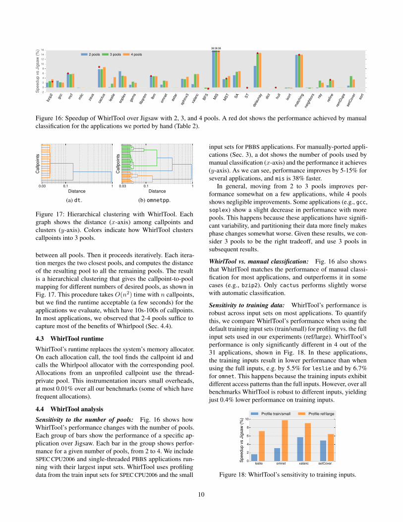
Figure 16: Speedup of WhirlTool over Jigsaw with 2, 3, and 4 pools. A red dot shows the performance achieved by manual
classification for the applications we ported by hand (Table 2).
0.03 0.1 1
Distance
Callp
oin
ts
(a) dt.
0.03 0.1 1
Distance
Callp
oin
ts
(b) omnetpp.
Figure 17: Hierarchical clustering with WhirlTool. Each
graph shows the distance (x-axis) among callpoints and
clusters (y-axis). Colors indicate how WhirlTool clusters
callpoints into 3 pools.
between all pools. Then it proceeds iteratively. Each itera-
tion merges the two closest pools, and computes the distance
of the resulting pool to all the remaining pools. The result
is a hierarchical clustering that gives the callpoint-to-pool
mapping for different numbers of desired pools, as shown in
Fig. 17. This procedure takes O(n2) time with n callpoints,
but we find the runtime acceptable (a few seconds) for the
applications we evaluate, which have 10s-100s of callpoints.
In most applications, we observed that 2-4 pools suffice to
capture most of the benefits of Whirlpool (Sec. 4.4).
4.3 WhirlTool runtime
WhirlTool’s runtime replaces the system’s memory allocator.
On each allocation call, the tool finds the callpoint id and
calls the Whirlpool allocator with the corresponding pool.
Allocations from an unprofiled callpoint use the thread-
private pool. This instrumentation incurs small overheads,
at most 0.01% over all our benchmarks (some of which have
frequent allocations).
4.4 WhirlTool analysis
Sensitivity to the number of pools: Fig. 16 shows how
WhirlTool’s performance changes with the number of pools.
Each group of bars show the performance of a specific ap-
plication over Jigsaw. Each bar in the group shows perfor-
mance for a given number of pools, from 2 to 4. We include
SPEC CPU2006 and single-threaded PBBS applications run-
ning with their largest input sets. WhirlTool uses profiling
data from the train input sets for SPEC CPU2006 and the small
input sets for PBBS applications. For manually-ported appli-
cations (Sec. 3), a dot shows the number of pools used by
manual classification (x-axis) and the performance it achieves
(y-axis). As we can see, performance improves by 5-15% for
several applications, and mis is 38% faster.
In general, moving from 2 to 3 pools improves per-
formance somewhat on a few applications, while 4 pools
shows negligible improvements. Some applications (e.g., gcc,
soplex) show a slight decrease in performance with more
pools. This happens because these applications have signifi-
cant variability, and partitioning their data more finely makes
phase changes somewhat worse. Given these results, we con-
sider 3 pools to be the right tradeoff, and use 3 pools in
subsequent results.
WhirlTool vs. manual classification: Fig. 16 also shows
that WhirlTool matches the performance of manual classi-
fication for most applications, and outperforms it in some
cases (e.g., bzip2). Only cactus performs slightly worse
with automatic classification.
Sensitivity to training data: WhirlTool’s performance is
robust across input sets on most applications. To quantify
this, we compare WhirlTool’s performance when using the
default training input sets (train/small) for profiling vs. the full
input sets used in our experiments (ref/large). WhirlTool’s
performance is only significantly different in 4 out of the
31 applications, shown in Fig. 18. In these applications,
the training inputs result in lower performance than when
using the full inputs, e.g. by 5.5% for leslie and by 6.7%
for omnet. This happens because the training inputs exhibit
different access patterns than the full inputs. However, over all
benchmarks WhirlTool is robust to different inputs, yielding
just 0.4% lower performance on training inputs.
leslie omnet xalanc setCover0
2
4
6
8
10
Sp
ee
du
p v
s J
igsa
w (
%)
Profile train/small Profile ref/large
Figure 18: WhirlTool’s sensitivity to training inputs.
10
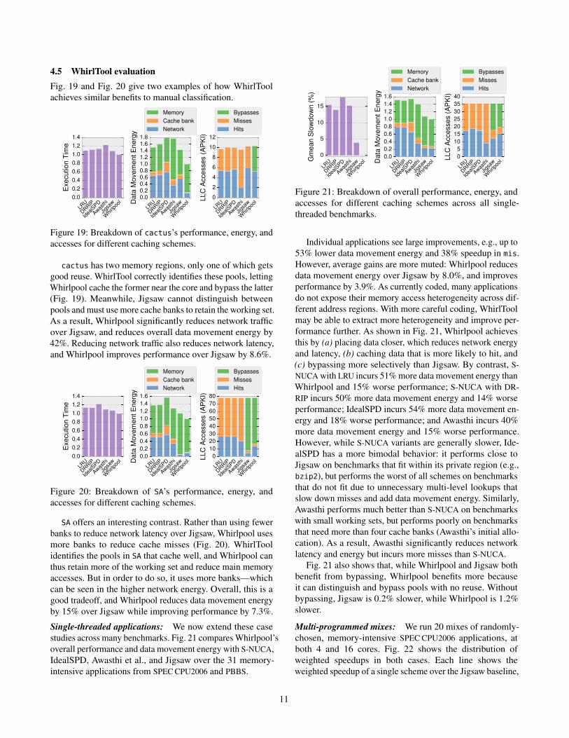
4.5 WhirlTool evaluation
Fig. 19 and Fig. 20 give two examples of how WhirlTool
achieves similar benefits to manual classification.
LRU
DRRIP
Idea
lSPD
Awas
thi
Jigs
aw
Whirlp
ool
0.0
0.2
0.4
0.6
0.8
1.0
1.2
1.4
Execution T
ime
LRU
DRRIP
Idea
lSPD
Awas
thi
Jigs
aw
Whirlp
ool
0.00.20.40.60.81.01.21.41.61.8
Data
Movem
ent E
nerg
y
Memory
Cache bank
Network
LRU
DRRIP
Idea
lSPD
Awas
thi
Jigs
aw
Whirlp
ool
0
2
4
6
8
10
12
LLC
Accesses (
AP
KI)
Bypasses
Misses
Hits
Figure 19: Breakdown of cactus’s performance, energy, and
accesses for different caching schemes.
cactus has two memory regions, only one of which gets
good reuse. WhirlTool correctly identifies these pools, letting
Whirlpool cache the former near the core and bypass the latter
(Fig. 19). Meanwhile, Jigsaw cannot distinguish between
pools and must use more cache banks to retain the working set.
As a result, Whirlpool significantly reduces network traffic
over Jigsaw, and reduces overall data movement energy by
42%. Reducing network traffic also reduces network latency,
and Whirlpool improves performance over Jigsaw by 8.6%.
LRU
DRRIP
Idea
lSPD
Awas
thi
Jigs
aw
Whirlp
ool
0.0
0.2
0.4
0.6
0.8
1.0
1.2
1.4
Execution T
ime
LRU
DRRIP
Idea
lSPD
Awas
thi
Jigs
aw
Whirlp
ool
0.0
0.2
0.4
0.6
0.8
1.0
1.2
1.4
1.6
Data
Movem
ent E
nerg
y
Memory
Cache bank
Network
LRU
DRRIP
Idea
lSPD
Awas
thi
Jigs
aw
Whirlp
ool
0
10
20
30
40
50
60
70
80
LLC
Accesses (
AP
KI)
Bypasses
Misses
Hits
Figure 20: Breakdown of SA’s performance, energy, and
accesses for different caching schemes.
SA offers an interesting contrast. Rather than using fewer
banks to reduce network latency over Jigsaw, Whirlpool uses
more banks to reduce cache misses (Fig. 20). WhirlTool
identifies the pools in SA that cache well, and Whirlpool can
thus retain more of the working set and reduce main memory
accesses. But in order to do so, it uses more banks—which
can be seen in the higher network energy. Overall, this is a
good tradeoff, and Whirlpool reduces data movement energy
by 15% over Jigsaw while improving performance by 7.3%.
Single-threaded applications: We now extend these case
studies across many benchmarks. Fig. 21 compares Whirlpool’s
overall performance and data movement energy with S-NUCA,
IdealSPD, Awasthi et al., and Jigsaw over the 31 memory-
intensive applications from SPEC CPU2006 and PBBS.
LRU
DRRIP
Idea
lSPD
Awas
thi
Jigs
aw
Whirlp
ool
0
5
10
15
Gm
ean S
low
dow
n (
%)
LRU
DRRIP
Idea
lSPD
Awas
thi
Jigs
aw
Whirlp
ool
0.0
0.2
0.4
0.6
0.8
1.0
1.2
1.4
1.6
Data
Movem
ent E
nerg
y
Memory
Cache bank
Network
LRU
DRRIP
Idea
lSPD
Awas
thi
Jigs
aw
Whirlp
ool
0
5
10
15
20
25
30
35
40
LLC
Accesses (
AP
KI)
Bypasses
Misses
Hits
Figure 21: Breakdown of overall performance, energy, and
accesses for different caching schemes across all single-
threaded benchmarks.
Individual applications see large improvements, e.g., up to
53% lower data movement energy and 38% speedup in mis.
However, average gains are more muted: Whirlpool reduces
data movement energy over Jigsaw by 8.0%, and improves
performance by 3.9%. As currently coded, many applications
do not expose their memory access heterogeneity across dif-
ferent address regions. With more careful coding, WhirlTool
may be able to extract more heterogeneity and improve per-
formance further. As shown in Fig. 21, Whirlpool achieves
this by (a) placing data closer, which reduces network energy
and latency, (b) caching data that is more likely to hit, and
(c) bypassing more selectively than Jigsaw. By contrast, S-
NUCA with LRU incurs 51% more data movement energy than
Whirlpool and 15% worse performance; S-NUCA with DR-
RIP incurs 50% more data movement energy and 14% worse
performance; IdealSPD incurs 54% more data movement en-
ergy and 18% worse performance; and Awasthi incurs 40%
more data movement energy and 15% worse performance.
However, while S-NUCA variants are generally slower, Ide-
alSPD has a more bimodal behavior: it performs close to
Jigsaw on benchmarks that fit within its private region (e.g.,
bzip2), but performs the worst of all schemes on benchmarks
that do not fit due to unnecessary multi-level lookups that
slow down misses and add data movement energy. Similarly,
Awasthi performs much better than S-NUCA on benchmarks
with small working sets, but performs poorly on benchmarks
that need more than four cache banks (Awasthi’s initial allo-
cation). As a result, Awasthi significantly reduces network
latency and energy but incurs more misses than S-NUCA.
Fig. 21 also shows that, while Whirlpool and Jigsaw both
benefit from bypassing, Whirlpool benefits more because
it can distinguish and bypass pools with no reuse. Without
bypassing, Jigsaw is 0.2% slower, while Whirlpool is 1.2%
slower.
Multi-programmed mixes: We run 20 mixes of randomly-
chosen, memory-intensive SPEC CPU2006 applications, at
both 4 and 16 cores. Fig. 22 shows the distribution of
weighted speedups in both cases. Each line shows the
weighted speedup of a single scheme over the Jigsaw baseline,
11
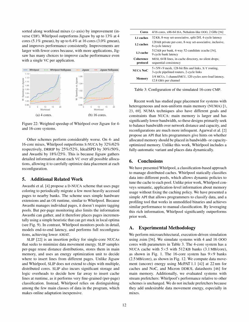
sorted along workload mixes (x-axis) by improvement (in-
verse CDF). Whirlpool outperforms Jigsaw by up to 13% at 4
cores (5.1% gmean), by up to 6.4% at 16 cores (3.0% gmean),
and improves performance consistently. Improvements are
larger with fewer cores because, with more applications, Jig-
saw has many choices to improve cache performance even
with a single VC per application.
Whirlpool Whirlpool-NoBypass Jigsaw Jigsaw-NoBypass
0 5 10 15 20
Workload
0.98
1.00
1.02
1.04
1.06
1.08
1.10
1.12
1.14
W. S
peedup v
s J
igsaw
(a) 4 cores.
0 5 10 15 20
Workload
0.98
1.00
1.02
1.04
1.06W
. S
peedup v
s J
igsaw
(b) 16 cores.
Figure 22: Weighted speedup of Whirlpool over Jigsaw for 4-
and 16-core systems.
Other schemes perform considerably worse. On 4- and
16-core mixes, Whirlpool outperforms S-NUCA by 32%/62%
respectively, DRRIP by 25%/52%, IdealSPD by 30%/50%,
and Awasthi by 18%/25%. This is because Jigsaw gathers
detailed information about each VC over all possible alloca-
tions, allowing it to carefully optimize data placement at each
reconfiguration.
5. Additional Related Work
Awasthi et al. [4] propose a D-NUCA scheme that uses page
coloring to periodically migrate a few most heavily accessed
pages to nearby banks. The scheme uses simple hardware
extensions and an OS runtime, similar to Whirlpool. Because
Awasthi manages individual pages, it doesn’t require tagging
pools. But per-page monitoring also limits the information
Awasthi can gather, and it therefore places pages incremen-
tally using a simple heuristic that can get stuck in local optima
(see Fig. 9). In contrast, Whirlpool monitors pools in detail,
models end-to-end latency, and performs full reconfigura-
tions, achieving lower AMAT.
SLIP [22] is an insertion policy for single-core NUCAs
that seeks to minimize data movement energy. SLIP samples
per-page reuse distance distributions, stores them in main
memory, and uses an energy optimization unit to decide
where to insert lines from different pages. Unlike Jigsaw
and Whirlpool, SLIP does not extend to chips with multiple,
distributed cores. SLIP also incurs significant storage and
logic overheads to decide how far away to insert cache
lines at runtime, as it performs very fine-grained (per-page)
classification. Instead, Whirlpool relies on distinguishing
among the few main classes of data in the program, which
makes online adaptation inexpensive.
Cores 4/16 cores, x86-64 ISA, Nehalem-like OOO, 2 GHz [56]
L1 caches 32 KB, 8-way set-associative, split D/I, 4-cycle latency
L2 caches128 KB private per-core, 8-way set-associative, inclusive,
6-cycle latency
L3 cache512 KB per bank, 4-way 52-candidate zcache [54],
9 cycle bank latency
Coherence
protocol
MESI, 64 B lines, in-cache directory, no silent drops;
sequential consistency
NUCA NoC5×5/9×9 mesh, 128-bit flits and links, X-Y routing,
3-cycle pipelined routers, 2-cycle links
Memory1/4 MCUs, 1 channel/MCU, 120 cycles zero-load latency,
12.8 GB/s per channel
Table 3: Configuration of the simulated 16-core CMP.
Recent work has studied page placement for systems with
heterogeneous and non-uniform main memory (NUMA) [1,
23, 69]. NUMA techniques also have different goals and
constraints than NUCA: main memory is larger and has
significantly lower bandwidth, so these designs primarily seek
to balance bandwidth over network distance and capacity, and
reconfigurations are much more infrequent. Agarwal et al. [2]
propose an API that lets programmers give hints on whether
allocated memory should be placed in bandwidth- or capacity-
optimized memory. Unlike this work, Whirlpool includes a
fully-automatic variant and places data dynamically.
6. Conclusions
We have presented Whirlpool, a classification-based approach
to manage distributed caches. Whirlpool statically classifies
data into different pools, which allows dynamic policies to
tune the cache to each pool. Unlike prior work, Whirlpool con-
veys semantic, application-level information about memory
usage without fixing the caching policy. We have presented a
simple API that allows programmers to classify data, and a
profiling tool that works in unmodified binaries and achieves
similar performance to manual classification. By leveraging
this rich information, Whirlpool significantly outperforms
prior work.
A. Experimental Methodology
We perform microarchitectural, execution-driven simulation
using zsim [56]. We simulate systems with 4 and 16 OOO
cores with parameters in Table 3. The 4-core system has a
NUCA cache with 5×5 with 512 KB banks (3.1 MB/core),
as shown in Fig. 1. The 16-core system has 9×9 banks
(2.5 MB/core), as shown in Fig. 12. We compute data move-
ment (uncore) energy using McPAT 1.1 [42] at 22 nm for
caches and NoC, and Micron DDR3L datasheets [46] for
main memory. Additionally, we evaluated systems with
stream prefetchers: Whirlpool’s performance relative to other
schemes is unchanged. We do not include prefetchers because
they add undesirable data movement energy, especially in
mixes.
12
We compare Whirlpool with D-NUCA and S-NUCA con-
figurations. Jigsaw and Whirlpool both use latency-aware ca-
pacity allocation and trading data placement [11]. For private-
baseline D-NUCAs, we model an idealized shared-private
D-NUCA scheme, IdealSPD, which we grant additional ca-
pacity. In IdealSPD, each core has a private 1.5 MB L3 that
replicates the 3 closest NUCA banks, followed by a fully-
provisioned directory and an exclusive, S-NUCA L4. L4 banks
act as a victim cache and are accessed in parallel with the di-
rectory to minimize latency. IdealSPD upper-bounds D-NUCA
schemes that partition the LLC between private and shared re-
gions, as private (L3) regions do not reduce the capacity of the
shared (L4) region. Herrero et al. [30] show that this idealized
scheme always outperforms several state-of-the-art private-
baseline D-NUCA schemes that include shared-private parti-
tioning, selective replication, and adaptive spilling (DCC [29],
ASR [6], and ECC [30]), often significantly (up to 30%). For
shared-baseline D-NUCAs, we compare against Awasthi et
al. [4], discussed in Sec. 5. We have implemented Awasthi
as proposed, sweeping implementation parameters αA, αB
to find the values that perform best. Other shared-baseline
D-NUCAs use placement heuristics that compare unfavor-
ably to Awasthi and Whirlpool; e.g., R-NUCA [28] achieves
6.8%/7.2% lower performance than Awasthi on 4-/16-core
mixes of SPEC CPU2006.
We use SPEC CPU2006 and PBBS [60] apps. In single-
program experiments, SPEC apps are executed for 10 B in-
structions after fast-forwarding 20 B instructions, and PBBS
apps are fast-forwarded to the start of their region of inter-
est, and run for the full region. We consider the applica-
tions with >5 L2 MPKI: 15 from SPEC CPU2006 (bzip2,
gcc, mcf, milc, zeusmp, cactusADM, leslie3d, soplex,
GemsFDTD, libquantum, lbm, astar, omnetpp, sphinx3, and
xalancbmk) and 16 from PBBS (all but nbody).
We also simulate mixes of single-threaded SPEC CPU2006
apps, using a fixed-work methodology similar to prior
work [9, 31, 33]: we run random mixes with 1 B instruc-
tions per app after fast-forwarding for 20 B instructions. All
apps are kept running until all finish 1 B instructions, and we
only consider the first 1 B instructions of each app.
B. Modeling Combined Miss Rate Curves
As discussed in Sec. 4, WhirlTool’s distance metric needs to
estimate the combined miss rate curve of several callpoints.
Several prior models predict shared cache interference [15, 17,
25, 66], but these are somewhat complex and computationally
expensive. We instead develop a simpler model that lets
WhirlTool rapidly estimate the effect of combining pools.
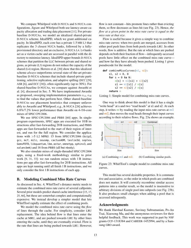
We model the combined miss rate curve using the flow
of lines through the cache. For simplicity, consider LRU
replacement. The idea behind flow is that lines enter the
cache at MRU, and are pushed towards LRU by other lines
entering the cache, until they are eventually evicted. Flow is
the rate that lines are being pushed towards LRU. However,
flow is not constant—hits promote lines rather than evicting
them, so flow decreases as lines hit (see Fig. 23). Hence, the
flow at a given point in the miss rate curve is equal to the
miss rate at that size.
Flow is useful because it gives a simple way to combine
miss rate curves: when two pools are merged, accesses from
either pool push lines from both pools towards LRU. In other
words, flow is additive. But the rate at which lines are pushed
depends on both their fraction of flow—infrequently-accessed
pools have little effect on the combined miss rate curve—
and how far they have already been pushed. Listing 1 gives
pseudocode for the model.
def combineMissCurves(m1, m2):
s1, s2 = 0, 0
for s = 0 to N:
m[s] = m1[s1] + m2[s2]
s1 += m1[s1] / m[s]
s2 += m2[s2] / m[s]
return m
Listing 1: Simple model for combining miss rate curves.
One way to think about this model is that it has a single
“write head” at s and two “read heads” at s1 and s2. At each
step, it writes m by reading the input miss rate curves at m1
and m2, then moves the read heads through their input curves
according to their relative flows. Fig. 23a shows an example.
Size
Mis
s R
ate
(a) Combining m1 and m2.
Size
Mis
s R
ate
(b) Combining similar pools.
m1 m2 Combined
Figure 23: WhirlTool’s simple model to combine miss rate
curves.
This model has several desirable properties. It is commuta-
tive and associative, so the order in which pools are combined
does not matter. It will correctly recombine similar access
patterns into a similar result, so the model is insensitive to
arbitrary divisions of single pool into subpools (see Fig. 23b).
It also produces small changes when adding a pool that is
accessed infrequently.
Acknowledgments
We thank Harshad Kasture, Suvinay Subramanian, Po-An
Tsai, Xiaosong Ma, and the anonymous reviewers for their
helpful feedback. This work was supported in part by NSF
grants CCF-1318384 and CAREER-1452994, and by a Sam-
sung GRO award.
13
References
[1] N. Agarwal, D. Nellans, M. O’Connor, S. W. Keckler, and
T. F. Wenisch, “Unlocking bandwidth for GPUs in CC-NUMA
systems,” in Proc. HPCA-21, 2015.
[2] N. Agarwal, D. Nellans, M. Stephenson, M. O’Connor, and
S. W. Keckler, “Page Placement Strategies for GPUs within
Heterogeneous Memory Systems,” in Proc. ASPLOS-XX, 2015.
[3] K. Aingaran, D. Smentek, T. Wicki, S. Jairath, G. Konstadini-
dis, S. Leung et al., “M7: Oracle’s Next-Generation Sparc
Processor,” IEEE Micro, no. 2, 2015.
[4] M. Awasthi, K. Sudan, R. Balasubramonian, and J. Carter, “Dy-
namic hardware-assisted software-controlled page placement
to manage capacity allocation and sharing within large caches,”
in Proc. HPCA-15, 2009.
[5] S. Beamer, K. Asanovic, and D. Patterson, “The GAP bench-
mark suite,” arXiv:1508.03619 [cs.DC], 2015.
[6] B. M. Beckmann, M. R. Marty, and D. A. Wood, “ASR: Adap-
tive selective replication for CMP caches,” in Proc. MICRO-39,
2006.
[7] B. M. Beckmann and D. A. Wood, “Managing wire delay in
large chip-multiprocessor caches,” in Proc. MICRO-37, 2004.
[8] N. Beckmann, “Design and analysis of spatially-partitioned
shared caches,” Ph.D. dissertation, Massachusetts Institute of
Technology, 2015.
[9] N. Beckmann and D. Sanchez, “Jigsaw: Scalable software-
defined caches,” in Proc. PACT-22, 2013.
[10] N. Beckmann and D. Sanchez, “Talus: A Simple Way to
Remove Cliffs in Cache Performance,” in Proc. HPCA-21,
2015.
[11] N. Beckmann, P.-A. Tsai, and D. Sanchez, “Scaling Dis-
tributed Cache Hierarchies through Computation and Data
Co-Scheduling,” in Proc. HPCA-21, 2015.
[12] K. Beyls and E. D’Hollander, “Generating cache hints for
improved program efficiency,” J. Syst. Architect., vol. 51, no. 4,
2005.
[13] R. D. Blumofe and C. E. Leiserson, “Scheduling multithreaded
computations by work stealing,” J. ACM, vol. 46, no. 5, 1999.
[14] J. Brock, X. Gu, B. Bao, and C. Ding, “Pacman: Program-
assisted cache management,” in Proc. ISMM, 2013.
[15] D. Chandra, F. Guo, S. Kim, and Y. Solihin, “Predicting inter-
thread cache contention on a chip multi-processor architecture,”
in Proc. HPCA-11, 2005.
[16] Q. Chen, M. Guo, and H. Guan, “LAWS: locality-aware work-
stealing for multi-socket multi-core architectures,” in Proc.
ICS, 2014.
[17] X. E. Chen and T. M. Aamodt, “A first-order fine-grained
multithreaded throughput model,” in Proc. HPCA-15, 2009.
[18] Z. Chishti, M. D. Powell, and T. Vijaykumar, “Optimizing
replication, communication, and capacity allocation in CMPs,”
in Proc. ISCA-32, 2005.
[19] S. Cho and L. Jin, “Managing distributed, shared L2 caches
through OS-level page allocation,” in Proc. MICRO-39, 2006.
[20] S. Coleman and K. S. McKinley, “Tile size selection using
cache organization and data layout,” in Proc. PLDI, 1995.
[21] W. J. Dally, “GPU Computing: To Exascale and Beyond,” in
Supercomputing ’10, Plenary Talk, 2010.
[22] S. Das, T. M. Aamodt, and W. J. Dally, “SLIP: reducing wire
energy in the memory hierarchy,” in Proc. ISCA-42, 2015.
[23] M. Dashti, A. Fedorova, J. Funston, F. Gaud, R. Lachaize,
B. Lepers et al., “Traffic management: a holistic approach to
memory placement on NUMA systems,” in Proc. ASPLOS-
XVIII, 2013.
[24] C. Ding and Y. Zhong, “Predicting whole-program locality
through reuse distance analysis,” in Proc. PLDI, 2003.
[25] D. Eklov, D. Black-Schaffer, and E. Hagersten, “StatCC: a
statistical cache contention model,” in Proc. PACT-19, 2010.
[26] M. Frigo, C. E. Leiserson, and K. H. Randall, “The Implemen-
tation of the Cilk-5 Multithreaded Language,” in Proc. PLDI,
1998.
[27] X. Gu, T. Bai, Y. Gao, C. Zhang, R. Archambault, and C. Ding,
“P-OPT: Program-directed optimal cache management,” in
Proc. LCPC-21, 2008.
[28] N. Hardavellas, M. Ferdman, B. Falsafi, and A. Ailamaki,
“Reactive NUCA: near-optimal block placement and replication
in distributed caches,” in Proc. ISCA-36, 2009.
[29] E. Herrero, J. González, and R. Canal, “Distributed cooperative
caching,” in Proc. PACT-17, 2008.
[30] E. Herrero, J. González, and R. Canal, “Elastic cooperative
caching: an autonomous dynamically adaptive memory hierar-
chy for chip multiprocessors,” in Proc. ISCA-37, 2010.
[31] A. Hilton, N. Eswaran, and A. Roth, “FIESTA: A sample-
balanced multi-program workload methodology,” Proc. MoBS,
2009.
[32] A. Jaleel, W. Hasenplaugh, M. Qureshi, J. Sebot, S. Steely Jr,
and J. Emer, “Adaptive insertion policies for managing shared
caches,” in Proc. PACT-17, 2008.
[33] A. Jaleel, K. B. Theobald, S. C. Steely Jr, and J. Emer, “High
performance cache replacement using re-reference interval
prediction (RRIP),” in Proc. ISCA-37, 2010.
[34] N. P. Jouppi, “Improving direct-mapped cache performance
by the addition of a small fully-associative cache and prefetch
buffers,” in Proc. ISCA-17, 1990.
[35] G. Karypis and V. Kumar, “A fast and high quality multilevel
scheme for partitioning irregular graphs,” SIAM J. Sci. Comput.,
vol. 20, no. 1, 1998.
[36] S. W. Keckler, W. J. Dally, B. Khailany, M. Garland, and
D. Glasco, “GPUs and the future of parallel computing,” IEEE
Micro, no. 5, 2011.
[37] C. Kim, D. Burger, and S. W. Keckler, “An adaptive, non-
uniform cache structure for wire-delay dominated on-chip
caches,” in Proc. ASPLOS-X, 2002.
[38] R. Komuravelli, M. D. Sinclair, M. Kotsifakou, P. Srivastava,
S. V. Adve, and V. S. Adve, “Stash: Have your scratchpad and
cache it too,” in Proc. ISCA-42, 2015.
[39] M. D. Lam, E. E. Rothberg, and M. E. Wolf, “The cache
performance and optimizations of blocked algorithms,” in Proc.
ASPLOS-IV, 1991.
14
[40] D. Lea, “A memory allocator,” http://gee.cs.oswego.edu/dl/
html/malloc.html, 2000.
[41] J. Leverich, H. Arakida, A. Solomatnikov, A. Firoozshahian,
M. Horowitz, and C. Kozyrakis, “Comparing memory systems
for chip multiprocessors,” in Proc. ISCA-34, 2007.
[42] S. Li, J. H. Ahn, R. D. Strong, J. B. Brockman, D. M. Tullsen,
and N. P. Jouppi, “McPAT: an integrated power, area, and
timing modeling framework for multicore and manycore archi-
tectures,” in Proc. MICRO-42, 2009.
[43] J. Lira, C. Molina, and A. González, “LRU-PEA: A smart
replacement policy for non-uniform cache architectures on
chip multiprocessors,” in Proc. ICCD, 2009.
[44] C.-K. Luk, R. Cohn, R. Muth, H. Patil, A. Klauser, G. Lowney
et al., “Pin: building customized program analysis tools with
dynamic instrumentation,” in Proc. PLDI, 2005.
[45] A. A. Melkman, “On-line construction of the convex hull of
a simple polyline,” Information Processing Letters, vol. 25,
no. 1, 1987.
[46] Micron, “1.35V DDR3L power calculator (4Gb x16 chips),”
2013.
[47] T. C. Mowry, M. S. Lam, and A. Gupta, “Design and evaluation
of a compiler algorithm for prefetching,” in Proc. ASPLOS-V,
1992.
[48] S. Palanca, V. Pentkovski, S. Tsai, and S. Maiyuran, “Method
and apparatus for implementing non-temporal stores,” 2001,
US Patent 6,205,520.
[49] G. Pekhimenko, T. Huberty, R. Cai, O. Mutlu, P. B. Gibbons,
M. Kozuch et al., “Exploiting compressed block size as an
indicator of future reuse,” in Proc. HPCA-21, 2015.
[50] P. Petoumenos, G. Keramidas, and S. Kaxiras, “Instruction-
based reuse-distance prediction for effective cache manage-
ment,” in Proc. SAMOS, 2009.
[51] M. K. Qureshi, “Adaptive spill-receive for robust high-
performance caching in CMPs,” in Proc. HPCA-15, 2009.
[52] M. K. Qureshi and Y. N. Patt, “Utility-based cache partitioning:
A low-overhead, high-performance, runtime mechanism to
partition shared caches,” in Proc. MICRO-39, 2006.
[53] S. Rusu, H. Muljono, D. Ayers, S. Tam, W. Chen, A. Martin
et al., “Ivytown: A 22nm 15-core enterprise Xeon R© processor
family,” in Proc. ISSCC, 2014.
[54] D. Sanchez and C. Kozyrakis, “The ZCache: Decoupling ways
and associativity,” in Proc. MICRO-43, 2010.
[55] D. Sanchez and C. Kozyrakis, “Vantage: Scalable and efficient
fine-grain cache partitioning,” in Proc. ISCA-38, 2011.
[56] D. Sanchez and C. Kozyrakis, “ZSim: fast and accurate mi-
croarchitectural simulation of thousand-core systems,” in Proc.
ISCA-40, 2013.
[57] D. Sanchez, R. M. Yoo, and C. Kozyrakis, “Flexible architec-
tural support for fine-grain scheduling,” in Proc. ASPLOS-XV,
2010.
[58] N. Satish, N. Sundaram, M. M. A. Patwary, J. Seo, J. Park,
M. A. Hassaan et al., “Navigating the maze of graph analytics
frameworks using massive graph datasets,” in Proc. SIGMOD,
2014.[59] J. Shalf, S. Dosanjh, and J. Morrison, “Exascale computing
technology challenges,” in Proc. High Performance Computing
for Computational Science (VECPAR), 2010.
[60] J. Shun, G. E. Blelloch, J. T. Fineman, P. B. Gibbons, A. Kyrola,
H. V. Simhadri et al., “Brief announcement: the problem based
benchmark suite,” in Proc. SPAA, 2012.
[61] D. K. Tam, R. Azimi, L. B. Soares, and M. Stumm,
“RapidMRC: approximating L2 miss rate curves on commod-
ity systems for online optimizations,” in Proc. ASPLOS-XIV,
2009.
[62] G. Tyson, M. Farrens, J. Matthews, and A. R. Pleszkun,
“A modified approach to data cache management,” in Proc.
MICRO-28, 1995.
[63] Z. Wang, K. McKinley, A. L. Rosenberg, and C. C. Weems,
“Using the compiler to improve cache replacement decisions,”
in Proc. PACT-11, 2002.
[64] M. E. Wolf and M. S. Lam, “A data locality optimizing
algorithm,” in Proc. PLDI, 1991.
[65] C.-J. Wu, A. Jaleel, W. Hasenplaugh, M. Martonosi, S. C.
Steely Jr, and J. Emer, “SHiP: signature-based hit predictor for
high performance caching,” in Proc. MICRO-44, 2011.
[66] X. Xiang, B. Bao, C. Ding, and Y. Gao, “Linear-time modeling
of program working set in shared cache,” in Proc. PACT-20,
2011.
[67] R. M. Yoo, C. J. Hughes, C. Kim, Y.-K. Chen, and
C. Kozyrakis, “Locality-aware task management for unstruc-
tured parallelism: A quantitative limit study,” in Proc. SPAA,
2013.
[68] M. Zhang and K. Asanovic, “Victim replication: Maximizing
capacity while hiding wire delay in tiled chip multiprocessors,”
in Proc. ISCA-32, 2005.
[69] S. Zhuravlev, S. Blagodurov, and A. Fedorova, “Addressing
shared resource contention in multicore processors via schedul-
ing,” in Proc. ASPLOS-XV, 2010.
15