Whirlpool scenario of quintessence in thenon-minimal coupled scalar field cosmology

Orest Hrycyna and Marek Szyd lowski

Department of Theoretical Physics, Faculty of Philosophy, The John Paul IICatholic University of Lublin, Al. Rac lawickie 14, 20-950 Lublin, Poland

Astronomical Observatory, Jagiellonian University, Orla 171, 30-244 Krakow,Poland

Mark Kac Complex Systems Research Centre, Jagiellonian University, Reymonta4, 30-059 Krakow, Poland

September 17, 2009

Talk based on the following papers:

• Marek Szydlowski and Orest Hrycyna Scalar field cosmologyin the energy phase-space – unified description of dynamicsJCAP01(2009)039, arXiv:0811.1493 [astro-ph]

• Orest Hrycyna and Marek Szydlowski Twister quintessencescenario arXiv:0906.0335 [astro-ph]

Introduction

In the model under consideration we assume the spatially flat FRWuniverse filled with the non-minimally coupled scalar field andbarotropic fluid with the equation of the state coefficient wm. Theaction assumes following form

S =1

2

∫d4x√−g

(1

κ2R−ε

(gµν∂µφ∂νφ+ξRφ2

)−2U(φ)

)+Sm,

(1)where κ2 = 8πG , ε = +1,−1 corresponds to canonical andphantom scalar field, respectively, the metric signature is

(−,+,+,+), R = 6(

aa + a

a

)is the Ricci scalar, a is the scale

factor and a dot denotes differentiation with respect to thecosmological time and U(φ) is the scalar field potential function.Sm is the action for the barotropic matter part.

The dynamical equation for the scalar field we can obtain from thevariation δS/δφ = 0

φ+ 3Hφ+ ξRφ+ εU ′(φ) = 0, (2)

and energy conservation condition from the variation δS/δg = 0

E = ε1

2φ2 + ε3ξH2φ2 + ε3ξH(φ2) + U(φ) + ρm −

3

κ2H2. (3)

Then conservation conditions read3

κ2H2 = ρφ + ρm, (4)

H = −κ2

2

[(ρφ + pφ) + ρm(1 + wm)

](5)

where the energy density and the pressure of the scalar field are

ρφ = ε1

2φ2 + U(φ) + ε3ξH2φ2 + ε3ξH(φ2), (6)

pφ = ε1

2(1− 4ξ)φ2 − U(φ) + εξH(φ2)− ε2ξ(1− 6ξ)Hφ2 −(7)

ε3ξ(1− 8ξ)H2φ2 + 2ξφU ′(φ). (8)

Dynamical variables

In what follows we introduce the energy phase space variables

x ≡ κφ√6H

, y ≡κ√

U(φ)√3H

, z ≡ κ√6φ, (9)

which are suggested by the conservation condition

κ2

3H2ρφ +

κ2

3H2ρm = Ωφ + Ωm = 1 (10)

or in terms of the newly introduced variables

Ωφ = y 2 + ε[(1− 6ξ)x2 + 6ξ(x + z)2

]= 1− Ωm. (11)

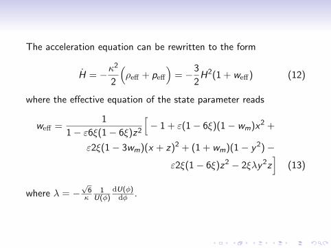
The acceleration equation can be rewritten to the form

H = −κ2

2

(ρeff + peff

)= −3

2H2(1 + weff) (12)

where the effective equation of the state parameter reads

weff =1

1− ε6ξ(1− 6ξ)z2

[− 1 + ε(1− 6ξ)(1− wm)x2 +

ε2ξ(1− 3wm)(x + z)2 + (1 + wm)(1− y 2)−

ε2ξ(1− 6ξ)z2 − 2ξλy 2z]

(13)

where λ = −√

6κ

1U(φ)

dU(φ)dφ .

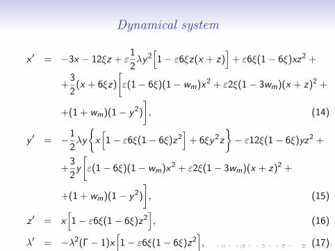
Dynamical system

x ′ = −3x − 12ξz + ε1

2λy 2

[1− ε6ξz(x + z)

]+ ε6ξ(1− 6ξ)xz2 +

+3

2(x + 6ξz)

[ε(1− 6ξ)(1− wm)x2 + ε2ξ(1− 3wm)(x + z)2 +

+(1 + wm)(1− y 2)

], (14)

y ′ = −1

2λy

x[1− ε6ξ(1− 6ξ)z2

]+ 6ξy 2z

− ε12ξ(1− 6ξ)yz2 +

+3

2y

[ε(1− 6ξ)(1− wm)x2 + ε2ξ(1− 3wm)(x + z)2 +

+(1 + wm)(1− y 2)

], (15)

z ′ = x[1− ε6ξ(1− 6ξ)z2

], (16)

λ′ = −λ2(Γ− 1)x[1− ε6ξ(1− 6ξ)z2

], (17)

where Γ =d2U(φ)

dφ2 U(φ)(dU(φ)dφ

)2 and prime denotes differentiation with

respect to time τ defined as

ddτ

=[1− ε6ξ(1− 6ξ)z2

] dd ln a

. (18)

If λ is constant then we obtain the scaling potential exp (λφ) andthe basic system reduces to the 3-dimensional autonomousdynamical system in the case of the model with the barotropicmatter. In the case without the matter the dynamical system is a2-dimensional autonomous one.

We will assume the following form of the function Γ(λ)

Γ(λ) = 1− α

λ2(19)

where α is an arbitrary constant and for which we can simplyeliminate one of the variables namely z given by the relation

z(λ) = −∫

dλλ2(Γ(λ)− 1

) =λ

α+ const (20)

and we take the integration constant as equal to zero.

From equation (19) and the definition of the function Γ we cansimply calculate the form of the potential function

U(φ) = U0 exp

[− κ2

6

(α

2φ2 + βφ

)]= U0 exp

[− (φ+ γ)2

](21)

where β is the integration constant. As we can see the dynamics ofthe model does not depend on the value of this parameter. In sucha case we are exploring the solutions in the very rich family ofpotential functions.

Following the Hartman-Grobman theorem the system can be wellapproximated by the linear part of the system around anon-degenerate critical point. Then stability of the critical point isdetermined by eigenvalues of a linearization matrix only. In Table 1we have gathered critical points appearing in whirlpool scenariotogether with the eigenvalues of the linearization matrix calculatedat those points.

Table: The location and eigenvalues of the critical points in whirlpool scenario

weff location eigenvalues

1. 13

x∗1 = 0, y∗1 = 0, (λ∗1 )2 = α2

ε6ξl1 = −6ξ, l2 = 12ξ, l3 = 6ξ(1− 3wm)

2. wm x∗2 = 0, y∗2 = 0, λ∗2 = 0 l1,3 = − 34

(1− wm)“

1±r

1− 163ξ 1−3wm

(1−wm)2

”, l2 = 3

2(1 + wm)

3. −1 x∗3 = 0, (y∗3 )2 = 1, λ∗3 = 0 l1,3 = − 12

“3±√

9 + ε2α− 48ξ”, l2 = −3(1 + wm)

The critical point of a saddle type which represents the radiationdominated universe weff = 1/3 is (x∗1 = 0, y∗1 = 0, (λ∗1)2 = α2

ε6ξ ) andthe linearized solutions in the vicinity of this critical point are

x1(a) =1

2− 3wm

[x

(i)1 −

1

α(1− 3wm)(λ

(i)1 − λ

∗1)]a−1 +

+(1− 3wm)[x

(i)1 +

1

α(λ

(i)1 − λ

∗1)]a1−3wm

, (22)

y1(a) = y(i)1 a2, (23)

λ1(a) = λ∗1 −α

2− 3wm

[x

(i)1 −

1

α(1− 3wm)(λ

(i)1 − λ

∗1)]a−1 −

−[x

(i)1 +

1

α(λ

(i)1 − λ

∗1)]a1−3wm

. (24)

In the case of canonical scalar field ε = +1 this critical point existsonly if ξ > 0 and for the phantom scalar field ε = −1 if ξ < 0.

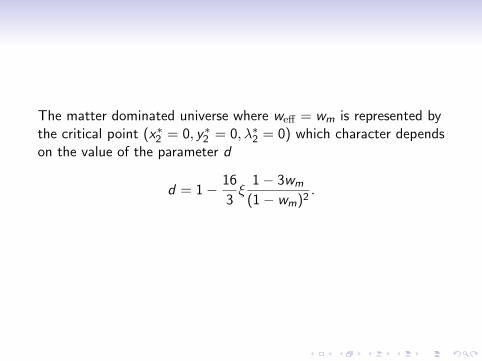
The matter dominated universe where weff = wm is represented bythe critical point (x∗2 = 0, y∗2 = 0, λ∗2 = 0) which character dependson the value of the parameter d

d = 1− 16

3ξ

1− 3wm

(1− wm)2.

For d > 0 the critical point is of a saddle type and the linearizedsolutions are in the form

x2(a) = a− 3

4 (1−wm)

2√

d

[(1+√

d)

[x

(i)2 + 1

α34

(1−wm)(1−√

d)λ(i)2

]a−

34 (1−wm)

√d−

−(1−√

d)

[x

(i)2 + 1

α34

(1−wm)(1+√

d)λ(i)2

]a

34 (1−wm)

√d

], (25)

y2(a) = y(i)2 a

32 (1+wm), (26)

λ2(a) = − 2αa− 3

4 (1−wm)

3(1−wm)√

d

[[x

(i)2 + 1

α34

(1−wm)(1−√

d)λ(i)2

]a−

34 (1−wm)

√d−

−[x

(i)2 + 1

α34

(1−wm)(1+√

d)λ(i)2

]a

34 (1−wm)

√d

]. (27)

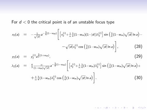
For d < 0 the critical point is of an unstable focus type

x2(a) = − 1√|d|

a−34 (1−wm)

[[x

(i)2 + 1

α34

(1−wm)(1−|d |)λ(i)2

]sin(

34

(1−wm)√|d | ln a

)−

−√|d |x(i)

2 cos(

34

(1−wm)√|d | ln a

)], (28)

y2(a) = y(i)2 a

32 (1+wm), (29)

λ2(a) = 43

α

(1−wm)√|d|

a−34 (1−wm)

[[x

(i)2 + 1

α34

(1−wm)λ(i)2

]sin(

34

(1−wm)√|d | ln a

)+

+ 1α

34

(1−wm)λ(i)2 cos

(34

(1−wm)√|d | ln a

)]. (30)

The final critical point represents the deSitter universe withweff = −1 is (x∗3 = 0, (y∗3 )2 = 1, λ∗3 = 0) its character depends onthe value of ∆ = 9 + ε2α− 48ξ.

For ∆ > 0 the critical point is of a stable node type and thelinearized solutions in the vicinity of this type critical points are

x3(a) =a−

32

2√

∆

(3 +

√∆)[x

(i)3 +

1

2α(3−

√∆)λ

(i)3

]a−√

∆2 −

−(3−√

∆)[x

(i)3 +

1

2α(3 +

√∆)λ

(i)3

]a√

∆2

, (31)

y3(a) = y∗3 + (y(i)3 − y∗3 )a−3(1+wm), (32)

λ3(a) = −αa−32

√∆

[x

(i)3 +

1

2α(3−

√∆)λ

(i)3

]a−√

∆2 −

−[x

(i)3 +

1

2α(3 +

√∆)λ

(i)3

]a√

∆2

. (33)

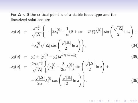
For ∆ < 0 the critical point is of a stable focus type and thelinearized solutions are

x3(a) =a−

32√|∆|

−[3x

(i)3 +

1

α(9 + εα− 24ξ)λ

(i)3

]sin

(√|∆|2

ln a

)+

+x(i)3

√|∆| cos

(√|∆|2

ln a

), (34)

y3(a) = y∗3 + (y(i)3 − y∗3 )a−3(1+wm), (35)

λ3(a) =2αa−

32√

|∆|

(x

(i)3 +

3

2αλ

(i)3

)sin

(√|∆|2

ln a

)+

+

√|∆|

2αλ

(i)3 cos

(√|∆|2

ln a

). (36)

The solutions of the linearized system in the vicinity of each criticalpoint xi (a), yi (a) and λi (a) can be used to constrain the modelparameters thorough the cosmological data from variouscosmological epochs. For example, the parameters for the solutiondescribing radiation dominated universe (1) can be constrainedfrom CMB data, and the solutions (3) describing the currentaccelerating expansion of the universe through the SN Ia data.Therefore one can estimate the parameters of the variability withredshift of true w(a) (see Fig.2). It is possible because we have thelinearization of exact formula in different epochs.

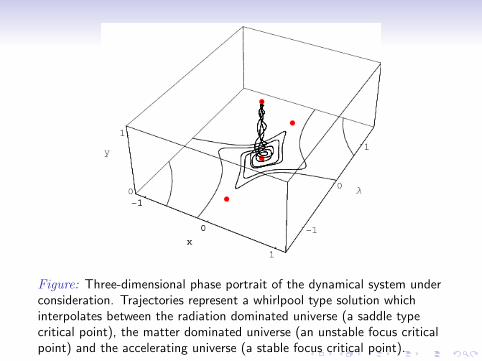
Figure: Three-dimensional phase portrait of the dynamical system underconsideration. Trajectories represent a whirlpool type solution whichinterpolates between the radiation dominated universe (a saddle typecritical point), the matter dominated universe (an unstable focus criticalpoint) and the accelerating universe (a stable focus critical point).

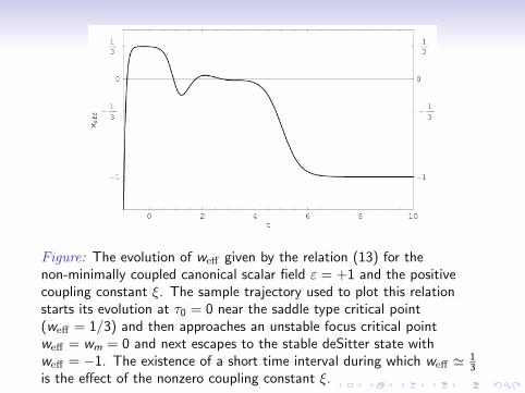
Figure: The evolution of weff given by the relation (13) for thenon-minimally coupled canonical scalar field ε = +1 and the positivecoupling constant ξ. The sample trajectory used to plot this relationstarts its evolution at τ0 = 0 near the saddle type critical point(weff = 1/3) and then approaches an unstable focus critical pointweff = wm = 0 and next escapes to the stable deSitter state withweff = −1. The existence of a short time interval during which weff ' 1

3is the effect of the nonzero coupling constant ξ.

The presented possibility of appearing whirlpool type quintessencescenario is not restricted to the considered case of the Γ(λ)function (19). One can easily show that such a scenario will bealways possible if only the following functions calculated at thecritical points

f (λ∗) = (λ∗)2(Γ(λ∗)− 1) = const,df (λ)

dλ|λ∗ = f ′(λ∗) = const

are finite.

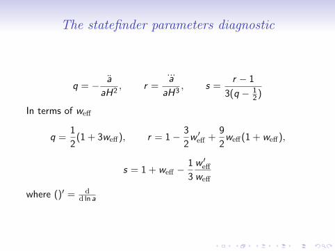
The statefinder parameters diagnostic

q = − a

aH2, r =

...a

aH3, s =

r − 1

3(q − 12 )

In terms of weff

q =1

2(1 + 3weff), r = 1− 3

2w ′eff +

9

2weff(1 + weff),

s = 1 + weff −1

3

w ′eff

weff

where ()′ = dd ln a

Figure: The time evolution of statefinder parameters (q, r) for whirlpoolscenario and different initial conditions. The red dots represent the valuesof (q, r) parameters for (from left) weff = −1, weff = 0, and weff = 1/3.The probing trajectories start with initial conditions close to the radiationdominated universe, then go to the point representing matter dominateduniverse and finally end in the deSitter state.

Conclusions

• We pointed out the presence of the new interesting solutionfor the non-minimally coupled scalar field cosmology which wecalled the whirlpool solution (because of the shape of thecorresponding trajectory in the phase space).

• This type of the solution is very interesting because in thephase space it represents the 3-dimensional trajectory whichinterpolates different stages of evolution of the universe,namely, the radiation dominated, dust filled and acceleratinguniverse.

• We found linearized solutions around all these intermediatephases, and hence, parameterizations for weff(a) in differentepochs of the universe history.

• It is interesting that the presented structure of the phasespace is allowed only for non-zero value of coupling constant,therefore it is a specific feature of the non-minimally coupledscalar field cosmology.