who benefits from the earned income tax credit? incidence among

DI

SC

US

SI

ON

P

AP

ER

S

ER

IE

S

Forschungsinstitut zur Zukunft der ArbeitInstitute for the Study of Labor

Who Benefi ts from the Earned Income Tax Credit? Incidence among Recipients, Coworkers and Firms

IZA DP No. 4960

May 2010

Andrew Leigh

Who Benefits from the

Earned Income Tax Credit? Incidence among Recipients,

Coworkers and Firms

Andrew Leigh Australian National University

and IZA

Discussion Paper No. 4960 May 2010

IZA

P.O. Box 7240 53072 Bonn

Germany

Phone: +49-228-3894-0 Fax: +49-228-3894-180

E-mail: [email protected]

Any opinions expressed here are those of the author(s) and not those of IZA. Research published in this series may include views on policy, but the institute itself takes no institutional policy positions. The Institute for the Study of Labor (IZA) in Bonn is a local and virtual international research center and a place of communication between science, politics and business. IZA is an independent nonprofit organization supported by Deutsche Post Foundation. The center is associated with the University of Bonn and offers a stimulating research environment through its international network, workshops and conferences, data service, project support, research visits and doctoral program. IZA engages in (i) original and internationally competitive research in all fields of labor economics, (ii) development of policy concepts, and (iii) dissemination of research results and concepts to the interested public. IZA Discussion Papers often represent preliminary work and are circulated to encourage discussion. Citation of such a paper should account for its provisional character. A revised version may be available directly from the author.

IZA Discussion Paper No. 4960 May 2010

ABSTRACT

Who Benefits from the Earned Income Tax Credit? Incidence among Recipients, Coworkers and Firms*

How are hourly wages affected by the Earned Income Tax Credit? Using variation in state EITC supplements, I find that a 10 percent increase in the generosity of the EITC is associated with a 5 percent fall in the wages of high school dropouts and a 2 percent fall in the wages of those with only a high school diploma, while having no effect on the wages of college graduates. Given the large increase in labor supply induced by the EITC, this is consistent with most reasonable estimates of the elasticity of labor demand. Although workers with children receive a much larger EITC than childless workers, and the effect of the credit on labor force participation is larger for those with children, the hourly wages of both groups are similarly affected by an EITC increase. As a check on this strategy, I also use federal variation in the EITC across gender-age-education groups, and find that those demographic groups that received the largest EITC increases also experienced a drop in their hourly wages, relative to other groups. JEL Classification: H22, H23, J22, J30 Keywords: taxation incidence, labor supply, simulated instrument Corresponding author: Andrew Leigh Research School of Economics Australian National University Canberra ACT 0200 Australia E-mail: [email protected]

* I am grateful to Anthony Atkinson, Jonathan Borck, David Cutler, David Ellwood, Doug Geyser, Richard Holden, Caroline Hoxby, Christopher Jencks, Lawrence Katz, Jeffrey Liebman, Adam Looney, Alexandre Mas, Casey Mulligan, Shanna Rose, Justin Wolfers, two anonymous referees, and seminar participants at Harvard University, the Public Policy Institute of California, the Society of Labor Economists annual conference, and Tufts University for helpful comments and suggestions. Thanks also to Raj Chetty, Dan Feenberg, Nicholas Johnson, Adam Looney, and Jesse Shapiro for advice in compiling federal and state policy parameters. Jenny Chesters and Susanne Schmidt provided outstanding research assistance.

2

1. Introduction The Earned Income Tax Credit (EITC) is the largest cash assistance program for low-wage workers in the United States. In 2008, federal EITC claims were projected to total $42.9 billion, with state EITC claims amounting to around $1.9 billion.1 But is the EITC a successful redistributive policy? Standard economic theory suggests that the effect of a tax change will be shared between employer and employee. If the EITC drives down gross wages, then an analysis that ignores wage changes will overestimate the impact of the policy on poverty and inequality. Substantial changes in EITC policy parameters over the past two decades provide a useful opportunity to estimate the incidence of the credit. Understanding how wages respond to the EITC is also relevant for the study of taxation incidence more generally.

Targeted at low-wage workers, the EITC has focused on achieving two major goals: distributing income towards low-wage workers, and increasing labor force participation rates. But there is most likely a tension between these objectives. If the EITC induces a net increase in labor supply, then unless labor demand is perfectly elastic, the equilibrium wage will fall (the impact of the EITC on wages is an echo of its effect on labor supply). Furthermore, if EITC-eligible and EITC-ineligible employees compete in the same labor market, a fall in the equilibrium wage will affect both groups. On net, ineligible workers will therefore be worse off than if the EITC had not been increased.

Perhaps because of these complications, the incidence of the EITC is an under-explored area. Reviewing the body of research on the EITC, Hotz and Scholz (2003) concluded: “We can think of no major EITC-related topic that has not had at least some attention from serious scholars, possibly with the exception of the economic incidence of the credit.”2 While the effect of the EITC on labor supply is well-documented, its impact on economic inequality is less clear. If gross wages fall with the introduction of an EITC, the policy will have less impact on post-tax inequality than if wages are unaffected.

Previous studies on the EITC have shown that the policy had a positive effect on the labor force participation of single women (see for example Eissa and Liebman 1996; Meyer and Rosenbaum 2001; Meyer 2002), and a small negative effect on the labor supply of low-skilled married women (Eissa and Hoynes

1 Federal data from Kuney and Levitis (2007). State EITCs are estimated by multiplying federal EITC claims for a state by its state EITC rate in 2008. I follow Kuney and Levitis (2007) in scaling the total down by a factor of 0.9, to account for underclaiming and for the fact that some credits are non-refundable. 2 Other valuable reviews of the EITC literature include Hoffman and Seidman (2002), Meyer and Holtz-Eakin (2002), and Eissa and Hoynes (2006).

3

2004). Using variation in state EITC supplements over the period 1985-1994, Neumark and Wascher (2001) found that an increase in a state’s EITC supplement significantly increased the household’s gross earned income.

The increases in employment induced by the EITC were sufficiently large that standard estimates of the elasticity of labor demand would lead one to expect considerable impacts on wages. For example, Meyer (2002) pointed out that in 1990-1997 (a period when the federal EITC was increased considerably), the employment of single mothers without a high school degree rose 22 percent. Suppose this increase was a pure supply shift, and these workers were not substitutable for other employees. Since the wage change is inversely proportional to the elasticity of labor demand, an elasticity of labor demand of -0.5 suggests that such an increase in labor supply should have led to a 44 percent reduction in the hourly wages of single mothers without a high school degree. The wage fall for this group would be lower if these workers are substitutable for other workers (since other employees would then share in the wage reduction). The wage fall for this group would also be lower if the elasticity of labor demand was larger (i.e. below -0.5).

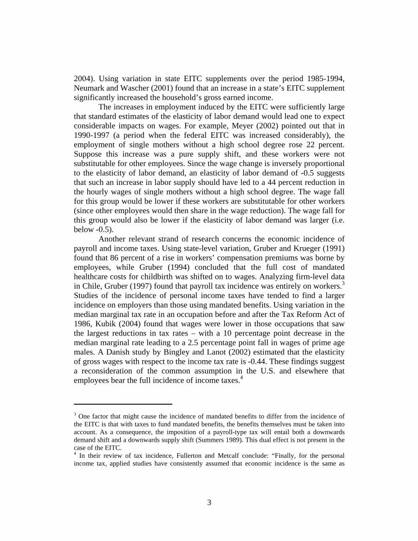
Another relevant strand of research concerns the economic incidence of payroll and income taxes. Using state-level variation, Gruber and Krueger (1991) found that 86 percent of a rise in workers’ compensation premiums was borne by employees, while Gruber (1994) concluded that the full cost of mandated healthcare costs for childbirth was shifted on to wages. Analyzing firm-level data in Chile, Gruber (1997) found that payroll tax incidence was entirely on workers.3 Studies of the incidence of personal income taxes have tended to find a larger incidence on employers than those using mandated benefits. Using variation in the median marginal tax rate in an occupation before and after the Tax Reform Act of 1986, Kubik (2004) found that wages were lower in those occupations that saw the largest reductions in tax rates – with a 10 percentage point decrease in the median marginal rate leading to a 2.5 percentage point fall in wages of prime age males. A Danish study by Bingley and Lanot (2002) estimated that the elasticity of gross wages with respect to the income tax rate is -0.44. These findings suggest a reconsideration of the common assumption in the U.S. and elsewhere that employees bear the full incidence of income taxes.4

3 One factor that might cause the incidence of mandated benefits to differ from the incidence of the EITC is that with taxes to fund mandated benefits, the benefits themselves must be taken into account. As a consequence, the imposition of a payroll-type tax will entail both a downwards demand shift and a downwards supply shift (Summers 1989). This dual effect is not present in the case of the EITC. 4 In their review of tax incidence, Fullerton and Metcalf conclude: “Finally, for the personal income tax, applied studies have consistently assumed that economic incidence is the same as

4

Two other studies (both drafted subsequently to this one) have estimated the impact of EITCs on wages. Focusing on a 1999 increase in the British EITC, Azmat (2006) found that for male recipients, 35 percent of the incidence of the credit is on the employer, and for female employees, the incidence is entirely on the employee. Azmat (2006) also found evidence of some spillover, with modest wage falls for non-recipient coworkers. Analyzing U.S. data from the 1990s, and restricting the sample to single women, Rothstein (2008) used a simulated instrument approach to estimate the impact of the federal EITC on hourly wages, exploiting variation across percentiles in the hourly wage distribution (an approach that adapts Di Nardo et al. 1996). Rothstein concluded that every $1 of EITC payments causes the wages of eligible workers to fall by $0.30 and the wages of ineligible workers to fall by $0.43.

In this paper, I use two strategies to estimate the effect of the EITC on gross wages. The first strategy exploits variation in state EITCs, under which certain states opted to ‘top up’ the federal EITC payment by as much as 75 percent. Using this source of variation, I find that a 10 percent increase in the generosity of the EITC is associated with a 5 percent drop in hourly wages for high school dropouts and a 2 percent fall in wages for those with only a high school diploma. The effect on hourly wages is similar for those with and without children, suggesting that what matters most is the mean eligibility in an individual’s labor market, not an individual’s own eligibility. As a check on these results, I approach the problem using an entirely different strategy – exploiting variation in the federal EITC across gender-age-education cells. Results from these specifications are consistent with the state-based results, suggesting that increasing the federal EITC also causes labor supply to rise and real hourly wages to fall.

The remainder of this paper is organized as follows. Section 2 reviews the structure and development of federal and state EITCs. Section 3 presents a simple model of the relationship between EITC rates and wages. Section 4 considers the net effect of changes in the EITC on hourly wages, using variation in state EITC supplements. Section 5 presents a different empirical specification – exploiting variation in the federal EITC across demographic groups. The final section concludes. 2. EITC structure and history Introduced in 1975, and significantly expanded in the late 1980s and 1990s, the EITC augments the earnings of low-wage workers. Based on family income, the credit has a phase-in range (in which the payment rises with earnings), a flat area statutory incidence – on the taxpayer – even though this assumption has never been tested” (2002, 29).

5

(in which the dollar value of the credit remains constant), and a phase-out range (in which the value of the credit diminishes until the credit phases out entirely). Prior to 1994, the credit was unavailable for taxpayers without dependent children, and remains substantially more generous for taxpayers with children.

Figure 1: Federal EITC Schedule - 2002

0

500

1000

1500

2000

2500

3000

3500

4000

4500

0 5000 10000 15000 20000 25000 30000 35000Annual Family Income ($)

EITC

pay

men

t ($)

Two children

One child

No children

Figure 1 shows the 2002 EITC parameters for families with no children, one child, and two or more children. In 2002, the maximum EITC payment for families with two children ($4140) was eleven times the size of the maximum payment for families with no children ($376). Table 1 shows the complete federal EITC rate schedule since 1984. Figure 2 shows the effect of the EITC on the budget constraint for one particular case – an unmarried taxpayer with one child in 2002.

The main strategy employed in this paper is to analyze state EITCs over the period 1989-2002. During this era, sixteen states (primarily in the Midwest and Northeast) and the District of Columbia implemented some form of state EITC supplement. Some provide a more generous state EITC supplement for larger families, and most are refundable for taxpayers with zero liability. All but one state EITC operated as a simple top-up to the federal EITC, such that the effective EITC rate was τ = (federal EITC rate)(1+state EITC supplement).5 For

5 The only state with an EITC not based on the federal credit is Indiana. In 1999-2002, Indiana had an EITC that was not based on the federal credit, but applied to families with children where

6

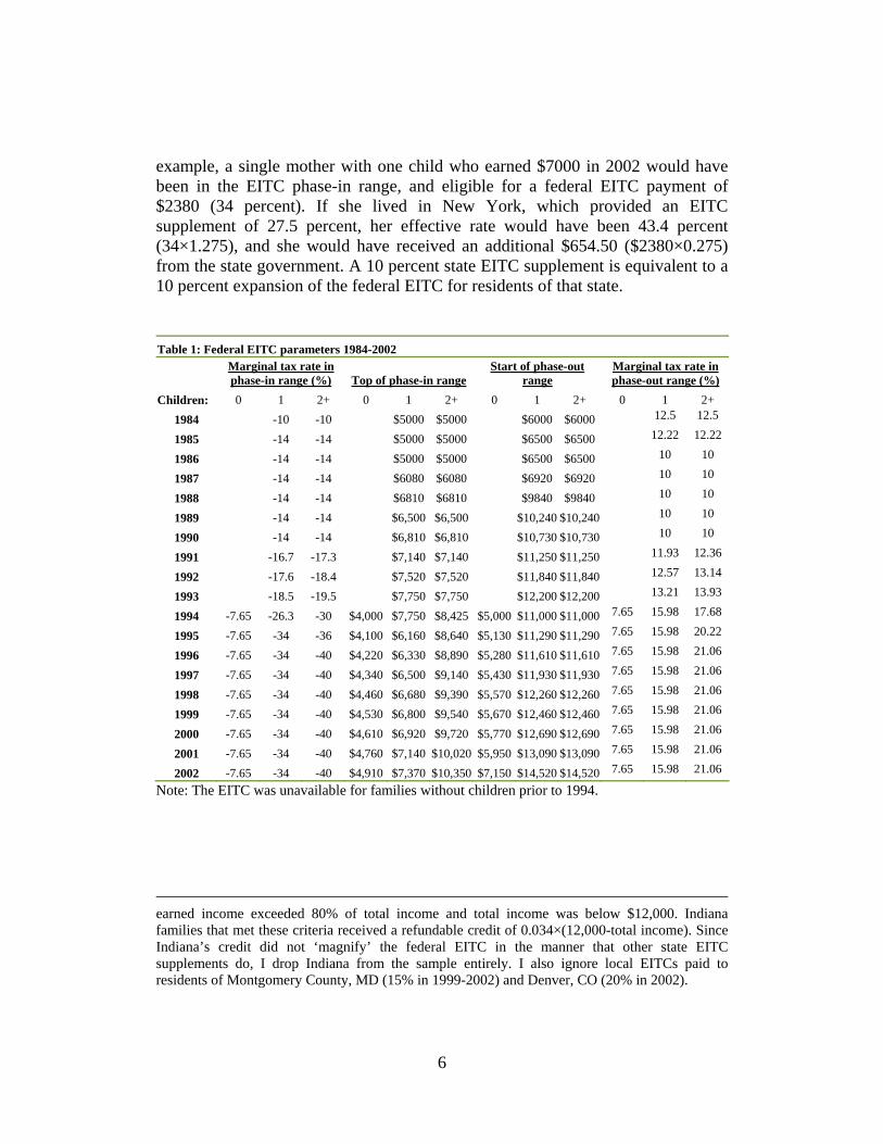
example, a single mother with one child who earned $7000 in 2002 would have been in the EITC phase-in range, and eligible for a federal EITC payment of $2380 (34 percent). If she lived in New York, which provided an EITC supplement of 27.5 percent, her effective rate would have been 43.4 percent (34×1.275), and she would have received an additional $654.50 ($2380×0.275) from the state government. A 10 percent state EITC supplement is equivalent to a 10 percent expansion of the federal EITC for residents of that state. Table 1: Federal EITC parameters 1984-2002

Marginal tax rate in phase-in range (%) Top of phase-in range

Start of phase-out range

Marginal tax rate in phase-out range (%)

Children: 0 1 2+ 0 1 2+ 0 1 2+ 0 1 2+ 1984 -10 -10 $5000 $5000 $6000 $6000 12.5 12.5

1985 -14 -14 $5000 $5000 $6500 $6500 12.22 12.22

1986 -14 -14 $5000 $5000 $6500 $6500 10 10

1987 -14 -14 $6080 $6080 $6920 $6920 10 10

1988 -14 -14 $6810 $6810 $9840 $9840 10 10

1989 -14 -14 $6,500 $6,500 $10,240 $10,240 10 10

1990 -14 -14 $6,810 $6,810 $10,730 $10,730 10 10

1991 -16.7 -17.3 $7,140 $7,140 $11,250 $11,250 11.93 12.36

1992 -17.6 -18.4 $7,520 $7,520 $11,840 $11,840 12.57 13.14

1993 -18.5 -19.5 $7,750 $7,750 $12,200 $12,200 13.21 13.93

1994 -7.65 -26.3 -30 $4,000 $7,750 $8,425 $5,000 $11,000 $11,000 7.65 15.98 17.68

1995 -7.65 -34 -36 $4,100 $6,160 $8,640 $5,130 $11,290 $11,290 7.65 15.98 20.22

1996 -7.65 -34 -40 $4,220 $6,330 $8,890 $5,280 $11,610 $11,610 7.65 15.98 21.06

1997 -7.65 -34 -40 $4,340 $6,500 $9,140 $5,430 $11,930 $11,930 7.65 15.98 21.06

1998 -7.65 -34 -40 $4,460 $6,680 $9,390 $5,570 $12,260 $12,260 7.65 15.98 21.06

1999 -7.65 -34 -40 $4,530 $6,800 $9,540 $5,670 $12,460 $12,460 7.65 15.98 21.06

2000 -7.65 -34 -40 $4,610 $6,920 $9,720 $5,770 $12,690 $12,690 7.65 15.98 21.06

2001 -7.65 -34 -40 $4,760 $7,140 $10,020 $5,950 $13,090 $13,090 7.65 15.98 21.06

2002 -7.65 -34 -40 $4,910 $7,370 $10,350 $7,150 $14,520 $14,520 7.65 15.98 21.06

Note: The EITC was unavailable for families without children prior to 1994.

earned income exceeded 80% of total income and total income was below $12,000. Indiana families that met these criteria received a refundable credit of 0.034×(12,000-total income). Since Indiana’s credit did not ‘magnify’ the federal EITC in the manner that other state EITC supplements do, I drop Indiana from the sample entirely. I also ignore local EITCs paid to residents of Montgomery County, MD (15% in 1999-2002) and Denver, CO (20% in 2002).

7

$0

$5,000

$10,000

$15,000

$20,000

$25,000

$30,000

$35,000

$40,000

Annual earnings

Annual hours

Figure 2: Budget Constraint - Single Taxpayer with One Child in 2002

Without EITCWith EITC

slope = w

slope = w

Assumes a single taxpayer with one child and no investment income, earning $10 per hour. Calculations based on Taxsim, and ignore all other taxes and credits. Note that the phase-in rate is negative, and phase-out rate is positive.

slope = w(1-phase-in rate)

slope = w(1-phase-out rate)

Table 2 provides details on state EITC supplements. While a few states provided EITC supplements in the 1980s, most were implemented in the mid to late 1990s. Johnson (2001) notes three factors that were important in the growth of state EITCs. First, under the Personal Responsibility and Work Opportunity Reconciliation Act of 1996, states were permitted to draw upon TANF block grants to partially fund an EITC. Second, welfare lobby groups pushed strongly for EITCs during this period. And third, state budget surpluses made EITCs fiscally feasible (indeed, Colorado and Maryland made expansions of their state EITCs contingent upon state revenue growth). States that enacted EITCs during the period 1989-2002 tended to be those in which Democrats won a higher share of the vote.6

6 In the 1992-2000 Presidential elections, Democrats won 57% of the vote in states that enacted an EITC between 1989 and 2002, but 51% of the vote in states that did not enact an EITC over this period (this is true whether Indiana is included or excluded).

Table 2: State EITC supplements 1984-2002 (%) State: CO DC IA IL KS MA MD ME MN MN NJ NY OK OR RI VT WI WI WI # of children: 1+ 0 1+ 1+ 1 2 3+

1984 30 30 30 1985 30 30 30 1986 22.21 1987 23.46 1988 22.96 23 1989 22.96 25 5 25 75 1990 5 22.96 28 5 25 75

1991 6.5 10 10 27.5 28 5 25 75

1992 6.5 10 10 27.5 28 5 25 75 1993 6.5 15 15 27.5 28 5 25 75

1994 6.5 15 15 7.5 27.5 25 4.4 20.8 62.5

1995 6.5 15 15 10 27.5 25 4 16 50

1996 6.5 15 15 20 27.5 25 4 14 43

1997 6.5 10 15 15 20 5 27.5 25 4 14 43

1998 6.5 10 10 10 15 25 20 5 27 25 4 14 43 1999 8.5 6.5 10 10 10 25 25 20 5 26.5 25 4 14 43

2000 10 10 6.5 5 10 10 15 5 25 25 10 22.5 5 26 32 4 14 43

2001 10 25 6.5 5 10 15 16 5 33 33 15 25 5 25.5 32 4 14 43

2002 0 25 6.5 5 15 15 16 5 33 33 17.5 27.5 5 5 25 32 4 14 43

Refundable? Y Y N N Y Y Y N Y Y Y Y Y N N Y Y Y Y Notes: 1. Maryland also had a non-refundable EITC of 50% for families with children from 1987-2002. 2. ‘Children’ is the number of children the taxpayer had to have in order to be eligible for the state EITC supplement. It is left blank if the

supplement applied irrespective of the taxpayer’s number of children. 3. Supplement is the percentage top-up of the federal EITC payment provided by the state. I ignore local EITCs implemented by Montgomery

County, MD and Denver, CO. 4. In 1999-2002, Indiana had an EITC which was not based on the federal EITC, and I therefore drop respondents from Indiana in those years.

9

Unlike payroll taxation rates, which are directly visible to employers, a worker’s EITC entitlement is essentially unobserved by employers. To determine eligibility, an employer would need to know the worker’s number of children, their estimated annual earnings from all jobs, and (if the worker is married) their spouse’s estimated annual earnings. This situation contrasts with the U.K., where the default payment option for the Working Families Tax Credit is via the pay packet, and both employers and workers can observe the value of the credit on a month-by-month basis. Although U.S. EITC recipients can also receive the credit in their pay packet, this option is utilized by fewer than 1 percent of recipients (U.S. Treasury 2003). 3. Modeling EITC incidence How should we expect the EITC to affect hourly wages?7 To model this, I assume a single labor market with one equilibrium wage and no other taxes. Suppose that there are two types of employees – those who are eligible for the EITC and those who are ineligible, and that each group is identical (this assumption will be relaxed later). Assume that employees place the same valuation on the EITC as they do on post-tax earnings.8 Using a standard semi-log formulation for labor supply, tax changes affect labor supply in two ways – through the marginal tax rate (the substitution effect) and through virtual income (the income effect). Consider first the marginal tax rate effect. Assuming EITC-induced changes in wages have no effect on prices, we can write the relationship between the post-tax wage (w) and the pre-tax wage (W) as:

( )τ−= 1Ww (1)

Taking natural logs of both sides, and differentiating:

ττ−

−=1d

WdW

wdw (2)

7 In this section, I model EITC recipients as responding to their marginal EITC rate. However, one might also imagine situations in which employees respond to their average rate, or even respond as though the EITC was a lump-sum reward for working. These non-standard models are explored in more detail in Leigh (2004). 8 Within a rational framework, this will be true only if the discount rate and the interest rate both equal zero. However, Romich and Weisner (2000) posit a behavioral model, suggesting that most recipients prefer to receive the EITC annually rather than monthly because it acts as a form of forced savings, allowing them to accumulate for durable goods purchases.

10

Note that τ is expressed as a marginal tax rate, so it will be negative in the EITC phase-in range, and positive in the EITC phase-out range. Now, recalling the relationship between total labor supply (LS), the uncompensated elasticity of labor supply (ηS), and the post-tax wage:

wdw

LdL

SS

S η≡ (3)

Equation (3) can be rewritten in terms of the pre-tax wage and the

marginal tax rate:

⎟⎠⎞

⎜⎝⎛

−−=

ττη

1d

WdW

LdL

SS

S (4)

Next, it is necessary to take account of the impact that virtual income has

on labor supply. Virtual income is defined as V≡(Y+U)-T-(1-τ)Y, where τ is the marginal tax rate, Y is annual earned income, T is total tax liability (note that tax liability will be negative for EITC recipients), and U is unearned income. This simplifies to V= τY-T+U. Where ζ is the income elasticity, we can add in the virtual income effect:

VdVd

WdW

LdL

SS

S ζττη +⎟

⎠⎞

⎜⎝⎛

−−=

1 (5)

At this point, models of tax incidence typically assume that taxation

revenue is returned to households in a lump sum fashion, and therefore that the income effect is zero. For payroll taxes and regular personal income taxes, this may be a reasonable assumption. However, because a negative income tax is a net transfer from the government to the individual (rather than the other way around), income effects are likely to be important. Moreover, while income and substitution effects operate in the same direction with positive income tax rates, the phase-in and phase-out rates of the EITC are such that income and substitution effects may operate in opposite directions.

If all employees are ineligible for the EITC, the change in labor supply will be:

WdW

LdL

SS

S η= (6)

11

If some fraction θ of the workforce is eligible for the EITC, the change in labor supply can be expressed as:

( )WdW

VdVd

WdW

LdL

SSS

S ηθζττηθ −+

⎭⎬⎫

⎩⎨⎧

+⎟⎠⎞

⎜⎝⎛

−−= 1

1 (7)

Assuming that eligible and ineligible workers are perfectly substitutable,

the relationship between total labor demand (LD), the elasticity of labor demand (ηD), and the pre-tax wage will be:

⎟⎠⎞

⎜⎝⎛≡

WdW

LdL

DD

D η (8)

Setting the change in labor supply equal to the change in labor demand

shows how the equilibrium wage will be affected by the introduction or expansion of a tax credit:

⎟⎟⎟⎟

⎠

⎞

⎜⎜⎜⎜

⎝

⎛

−

−−=

DS

S VdVd

WdW

ηη

ζττη

θ 1 (9)

Generalizing to a continuum of types with different marginal tax rates and

virtual incomes, equation (9) can be rewritten in terms of the average marginal EITC rate ( τ ) and the average virtual income ( V ):

DS

S VVdd

WdW

ηη

ζττη

−

−−= 1 (10)

Assuming that the elasticity of labor demand is negative, the elasticity of

labor supply is positive, and the income elasticity is negative, we can predict the effect on wages for the three regions of the EITC (recall that all eligibles are assumed to be identical, and therefore are in the same region of the EITC): • Phase-in region: The substitution effect will increase labor supply and reduce

wages, while the income effect will reduce labor supply and increase wages – so the net effect is indeterminate;

• Flat region: The substitution effect is zero, while the income effect will reduce labor supply and increase wages – so the net effect is an increase in wages;

12

• Phase-out region: The substitution effect and the income effect will both reduce labor supply and increase wages – so the net effect is an increase in wages.

(As noted above, most empirical studies of the impact on labor supply have found that the effect on the phase-in region dominates, and therefore that EITC expansions increase labor supply.) Note that under standard assumptions, the effect of the EITC on pre-tax hourly wages does not depend upon employers discerning whether employees are eligible or ineligible.9 The EITC simply causes a shift in labor supply, which then has a corresponding impact on the equilibrium wage. This wage change is inversely proportional to the elasticity of labor demand, such that dW/W=(dLS/LS)/ηD. For example, if the elasticity of labor demand is below -1 (as is often found in the immigration literature), then a policy that boosts labor supply by 1 percent will reduce wages by less than 1 percent.10 If the elasticity of labor demand is around -0.3 (as has been found in studies of the aggregate employment-wage elasticity), then a policy that boosts labor supply by 1 percent will reduce wages by 3.3 percent.11 And if the elasticity of labor demand is around -0.1 (as is often found in the minimum wage literature), then a policy that boosts labor supply by 1 percent will reduce wages by 10 percent.12 The less employment

9 This general rule might not hold in situations where employers had some information about workers’ EITC eligibility. For example, employers might seek to lower wages differentially if there was a prevailing belief that it would be ‘unfair’ for eligibles and ineligibles to have their wages change by the same amount (Bewley 2004). Another possibility is that employers wish to minimize job turnover, and therefore prefer to reduce wages for eligibles rather than ineligibles, since an indiscriminate wage reduction would cause the after-tax wage of some ineligibles to fall below their reservation wage, and they would therefore quit. 10 I have been unable to locate a meta-analysis in the immigration literature that summarizes the implied elasticity of labor demand, but one can obtain estimates by inverting the wage elasticity (this is inexact because wage elasticities typically hold marginal costs constant, while labor demand elasticities typically hold output constant). One oft-cited study is Borjas (2003), whose estimate of the wage elasticity (-0.3 to -0.4) implies a labor demand elasticity of approximately -2.5 to -3.3. Longhi et al. (2005) summarize 18 papers and conclude that the mean effect on wages of a 1 percentage point increase in migrant share is -0.119. Assuming that a 1 percentage point increase in migrant share increases labor supply by 1 percent, this translates into a labor demand elasticity of approximately -8.4. 11 Summarizing 28 published estimates from labor demand, production function and cost function studies, Hamermesh (1987) concluded that in developed economies in the 1960s to the 1980s, the aggregate long-run constant-output labor-demand elasticity lay in the range -0.15 to -0.50. 12 Among the most comprehensive surveys of labor demand elasticities in the minimum wage literature are Brown et al. (1982) and Neumark and Wascher (2007), which both include a substantial number of estimates around -0.1.

13

changes in response to an exogenous wage shock, the more wages will change in response to an exogenous labor supply shock.13 4. Exploiting variation from state EITCs The main strategy used in this paper to determine the incidence of the EITC is to exploit variation over time in state EITCs. In effect, this analysis estimates the change in labor market conditions when a state increases (or decreases) its EITC supplement. Econometrically, using state EITCs as a source of identification of labor market effects relies upon three main assumptions. The first is that the timing of state governments’ decisions to raise or lower the EITC is exogenous with respect to the state economy and other state policies. In section 4.1, I test whether state EITCs are associated with economic conditions and with various state policies. The second assumption is that each state can be regarded as a self-contained labor market, and that changes in EITCs do not induce interstate migration. This issue is addressed in section 4.4, in the context of compositional changes. The third assumption is that state EITCs have the same behavioral impact as the federal credit, an issue that I address in section 5 with a different identification strategy.

Since state EITC rates simply act as a supplement to the federal program, they should magnify the overall impact of the EITC on wages. However, because state EITC supplements augment the federal EITC by a fixed fraction, their impact will be larger in years when the federal EITC was more generous. It is therefore necessary to form a measure of the generosity of a state’s EITC in a given year. Because some states provide different EITC supplements according to family size, the generosity measure is a weighted average of the maximum EITC benefit available to a family with one child, two children and three or more children. The weights are simply derived from the approximate distribution of family sizes among those who have children, being 0.4 for one-child and two-child families, and 0.2 for three-child families: ρst = ln[0.4(Maximum 1-child EITC benefit)st + 0.4(Maximum 2-child EITC benefit)st + 0.2(Maximum 3-child EITC benefit)st]

13 The estimates in this paper are based on the labor markets of 1989-2002 (section 4) and 1984-2002 (section 5). The average unemployment rate in these periods is comparable to the mean in the postwar era. I am not aware of any work suggesting a relationship between the elasticity of labor demand and the business cycle, but there is some evidence that the labor supply elasticity is modestly counter-cyclical (see e.g. Gourio and Noual 2006). To the extent that my results are primarily driven by policy variation at a time of strong (weak) growth, this will understate (overstate) the expected labor supply impact in ordinary times.

14

I also test the robustness of these results to using an alternative measure of generosity: the maximum EITC benefit for a family with one child.

Figures 3-5 provide a visual sense of the econometric analysis to follow. In Figure 3, I plot for each state the change in the maximum EITC against the change in employment for high school dropouts. Since EITCs are more generous for workers with children than for those without children, the graphs show separate panels for each group. To ensure a sufficient sample size at the state-year level, the charts compare employment and wage rates in 1989-90 and 2001-02. The results suggest that, on average, increases in state EITC rates were associated with increases in employment for high school dropouts with children, but not for high school dropouts without children. In Figure 4, I repeat this exercise, looking at log weekly hours, and again find a larger increase in labor supply among high school dropouts with children. In Figure 5, I focus on hourly wages. In this case, both high school dropouts with children and those without children saw their hourly wages fall. This accords with the model in section 3: the employment changes occur only among adults with children, but the wage effects operate through the equilibrium wage, so affect those with and without children.

ME

NHVT

MA

RI

CT

NY

NJ

PAOHIL

MI

WI

MN

IA

MOND

SDNE

KSDE

MD

DCVAWV

NC

SCGAFLKYTNAL

MSARLA OK

TXMTIDWY

CO

NM

AZUT

NVWA

OR

CA

AK

HI

-.20

.2C

hang

e in

par

ticip

atio

n ra

te

.5 .6 .7 .8 .9Change in log EITC generosity

With Children

ME

NHVT

MA

RI

CT

NYNJPA

OH

ILMI

WI

MN

IAMO

ND

SD

NE

KS

DE

MD

DCVAWV

NCSC

GA

FL

KY

TN

AL

MS

AR

LA

OK

TXMT

ID

WY

CO

NM

AZ

UT

NV

WA

ORCAAK

HI

-.20

.2C

hang

e in

par

ticip

atio

n ra

te


Without Children

Charts show high school dropouts only. Change is from 1989/90 to 2001/02.Regression lines are weighted by sample size.

Figure 3: State EITCs and Employment

15

ME

NHVT

MA

RI

CT

NY

NJPA

OH

ILMI

WI

MN

IA

MO

ND

SDNE KS

DE

MD

DC

VA

WV

NC

SC

GA

FL

KYTNAL

MS

ARLA

OKTX

MT

ID

WY

CO

NM

AZUT

NV

WA

OR

CA

AK

HI

-.40

.4C

hang

e in

log

wee

kly

hour

s


With Children

ME

NH

VTMA

RI

CT

NYNJ

PA

OH

ILMIWI

MN

IA

MO

ND

SD

NE

KS

DE

MD DCVAWV

NCSC

GAFL

KY

TN

AL

MS

AR

LA

OK

TX

MT

ID

WY

CO

NM

AZUTNV

WA

ORCAAK

HI

-.40

.4C

hang

e in

log

wee

kly

hour

s


Without Children


Figure 4: State EITCs and Log Hours

MENH VT

MARI

CT

NYNJ

PAOH ILMI

WI

MN

IA

MO

ND

SD

NE

KS

DE MD DC

VA

WV

NCSCGA

FLKYTN

ALMS

AR

LA

OK

TX

MTID

WY

CO

NM

AZ

UT

NVWA ORCA

AK

HI

-.40

.4C

hang

e in

log

hour

ly w

age


With Children

MENH VT

MARI

CT

NYNJPA

OH

IL

MI

WIMN

IA

MO

ND

SD

NEKS

DE

MD

DCVAWVNCSCGA

FL

KY

TNAL

MS

AR

LA

OKTX

MT

IDWY

CONM

AZUTNV

WA

OR

CAAKHI

-.40

.4C

hang

e in

log

hour

ly w

age


Without Children


Figure 5: State EITCs and Hourly Wages

16

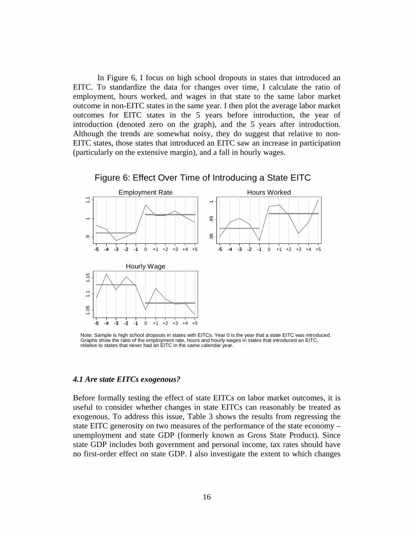
In Figure 6, I focus on high school dropouts in states that introduced an EITC. To standardize the data for changes over time, I calculate the ratio of employment, hours worked, and wages in that state to the same labor market outcome in non-EITC states in the same year. I then plot the average labor market outcomes for EITC states in the 5 years before introduction, the year of introduction (denoted zero on the graph), and the 5 years after introduction. Although the trends are somewhat noisy, they do suggest that relative to non-EITC states, those states that introduced an EITC saw an increase in participation (particularly on the extensive margin), and a fall in hourly wages.

.91

1.1

-5-5 -4-4 -3-3 -2-2 -1-1 0 +1 +2 +3 +4 +5

Employment Rate

.98

.99

1

-5-5 -4-4 -3-3 -2-2 -1-1 0 +1 +2 +3 +4 +5

Hours Worked

1.05

1.1

1.15

-5-5 -4-4 -3-3 -2-2 -1-1 0 +1 +2 +3 +4 +5

Hourly Wage

Note: Sample is high school dropouts in states with EITCs. Year 0 is the year that a state EITC was introduced.Graphs show the ratio of the employment rate, hours and hourly wages in states that introduced an EITC,relative to states that never had an EITC in the same calendar year.

Figure 6: Effect Over Time of Introducing a State EITC

4.1 Are state EITCs exogenous? Before formally testing the effect of state EITCs on labor market outcomes, it is useful to consider whether changes in state EITCs can reasonably be treated as exogenous. To address this issue, Table 3 shows the results from regressing the state EITC generosity on two measures of the performance of the state economy – unemployment and state GDP (formerly known as Gross State Product). Since state GDP includes both government and personal income, tax rates should have no first-order effect on state GDP. I also investigate the extent to which changes

17

in the EITC coincided with other state policies, by including in the regression the real minimum wage, three variables measuring welfare reform and generosity, the top state income tax rate, and variables indicating whether the state had introduced each of three electronic filing programs. Results are presented for two specifications – one in which the dependent variable is the current EITC level, and one in which the dependent variable is the EITC level in the next year. Both specifications include state and year fixed effects.

Only a handful of coefficients are significant at the 10 percent level, and none are significant at the 5 percent level. Only one variable – state GDP – is significantly related to state EITC generosity in both the contemporaneous and lagged regressions. On average, a 1 percent increase in state GDP is associated with a 0.1 percentage point increase in the state EITC supplement. This indicates that fast-growing states are more likely to introduce EITC supplements or raise their EITC supplements. To the extent that state GDP growth is positively correlated with wage growth, this suggests that failing to control for state GDP might lead to an overestimate of the share of the EITC received by the employee.

Table 3: Are state EITCs exogenous with respect to state economic performance? Dependent variable: Log Maximum

EITC in year t Log Maximum EITC in year

t+1 Log state GDP per capita 0.111* 0.090* [0.057] [0.050] Unemployment rate 0.04 0.055 [0.228] [0.226] Log real minimum wage 0.013 -0.016 [0.092] [0.097] Maximum AFDC/TANF benefit for a family of 3 -0.037* -0.019 [0.020] [0.021] Implemented welfare reform? 0.002 0.004 [0.008] [0.008] Obtained an AFDC waiver? -0.014 -0.015* [0.009] [0.009] Top state income tax rate -0.597 -1.251* [0.573] [0.702] State electronic filing program? -0.008 -0.006 [0.015] [0.014] State TeleFiling program? 0.009 0.009 [0.008] [0.009] Federal-state electronic filing program? 0.006 0.007 [0.015] [0.015] Observations 700 650 R-squared 0.98 0.98

Source: Author’s calculations, based on data from the 1989-2002 Current Population Surveys. Notes:

18

1. ***, **, and * denote significance at the 1%, 5%, and 10% levels respectively. Robust standard errors, clustered at the state level, in brackets. All specifications include state fixed effects and year fixed effects. I drop Indiana, since it had a state EITC that was not based on the federal credit.

2. Log maximum EITC is a weighted average of the maximum EITC benefit available to a family with one child (weight=0.4), two children (weight=0.4), and three or more children (weight=0.2).

Among the policy variables, I find that a 1 percent fall in welfare

generosity is associated with a 0.04 percent increase in the EITC (significant only in the contemporaneous specification). By contrast, when states were granted a federal waiver to experiment with provisions of the Aid to Families with Dependent Children program (AFDC), their state EITC supplement tended to fall by about 2 percentage points (significant only in the lagged specification). Since experimenting with AFDC typically involved making it harder to receive welfare, it is difficult to reconcile these two results, but it should be noted that they are significant in different specifications, and only at the 10 percent level.14

I also find that states with more generous EITCs tend to have lower top income tax rates: a 1 percentage point income tax rate cut is associated with a 1.3 percentage point rise in the value of the state’s EITC the following year (significant only in the lagged specification). This suggests that state policymakers tended to raise the EITC the year after they cut the top state tax rate. To the extent that lowering the top tax rate increased work incentives, this suggests that failing to control for it might lead me to overestimate the impact of state EITC supplements on boosting labor supply and reducing hourly wages. However, as with the welfare policy measures, the top tax rate is only significant at the 10 percent level.

To deal with the possibility that other factors are affecting state EITC rates, the labor supply and wage regressions control for all the policy variables listed in Table 3. As a robustness check, I also separately re-estimate the wage regressions controlling for state GDP.

14 Although these coefficients do not imply a strong relationship between state welfare policy and state EITCs, it is useful to acknowledge the sign of the potential bias that would arise if state policymakers tended to replace benefits for the non-working poor with in-work benefits. To the extent that cutting welfare raises the incentive to work, failing to adequately control for a fall in welfare generosity would lead me to overestimate the impact of state EITC supplements on boosting labor supply and reducing hourly wages.

19

4.2 State EITCs and labor supply Since the effect of the EITC on wages is an echo of the effect of the EITC on labor supply, it is useful to first estimate the effect of EITC generosity on labor supply.15 This involves estimating the following regression: LSist = α + βρst + δXist + πZst + ζs + λkt + εist (11)

where LS is a measure of labor supply (participation or log hours), ρ is the log of the maximum value of the EITC (weighted across family types), X is a set of demographic characteristics for the individual and their spouse, Z is a vector of time-varying state characteristics (the unemployment rate, the minimum wage, the top marginal state tax rate on wage income, welfare generosity, dummies for whether the state had ever obtained an AFDC waiver, implemented welfare reform, and for three types of e-filing programs), and ζ are state fixed effects. In specifications that pool individuals with and without children (Panels A and D), λ represents two vectors of year fixed effects – one for individuals with children, and one for individuals without children. This is a more stringent restriction than merely including one set of year dummies, since it allows time effects to operate differently for individuals with and without children. In specifications that include only parents, or only childless individuals (Panels B, C, E, and F), λ are simply year fixed effects. Standard errors are clustered at the state level, to take account of serial correlation (Bertrand et al. 2004).

Since few states provided EITC supplements during the 1980s, I restrict the sample to the 14-year period 1989-2002.16 Data are from the Current Population Survey Merged Outgoing Rotation Group, with the sample restricted to those aged 25-55 and not self-employed. Summary statistics and details on variable construction may be found in the Data Appendix.

Table 4 shows the relationship between the EITC and labor supply across different skill groups, with and without children. Panels A-C show the impact of the EITC on the extensive margin (employment), while panels D-F measure the impact on the intensive margin (log hours). The employment effect is estimated

15 As noted in section 3, the wage effects will depend not only upon whether the individual receives the EITC, but also whether his or her coworkers are EITC-eligible. I therefore estimate wage regressions using variation across states (rather than across eligible and ineligible workers). For ease of comparison, I use the same approach when estimating labor supply effects. (For the same reason, I do not estimate IV regressions in which state EITCs are used to instrument for an individual’s own EITC, since the wage effects are not confined to EITC-eligible individuals.) 16 Determining the appropriate point to begin the sample is necessarily somewhat arbitrary. The numbers of states with EITCs during the 1980s were: 1984-86: 1, 1987: 2, 1988: 3, 1989: 4 (note that these figures count Maryland’s non-refundable 50% EITC, which is not shown in Table 2).

20

using a linear probability model.17 Panel A shows that on the extensive margin, boosting the EITC has a significant positive effect on labor force participation, with the effect being strongest among low-skilled individuals. Decomposing this effect into its impact on individuals with and without children shows that the effect is stronger among adults with children. For all parents, a 10 percent rise in EITC generosity boosts the probability of employment by 0.6 percentage points. Most of this effect is concentrated among high school dropouts with children, for whom raising the EITC by 10 percent increases participation by 1.9 percentage points, and high school graduates with children, for whom boosting the EITC by 10 percent increases participation by 0.7 percentage points. There is no significant relationship between EITC generosity and employment among college graduates with children, nor for childless adults.

On the intensive margin, the effect of increasing the EITC is again positive and significant for all workers combined (Panel D). Separately analyzing the effect on parents (Panel E) shows that raising the generosity of the EITC by 10 percent leads to a 0.7 percent increase in log hours. Disaggregating the effect by skill groups, however, the effect on the hours worked of parents appears to be concentrated in the higher-skill groups. The absence of an observed hours effect among high school dropouts with children could be due to workers not being able to perfectly control their hours. It might also be due to compositional changes – if those who enter the labor market work fewer hours than those already in the labor force, this will bring down the average number of hours for that group, making it more difficult to discern the impact on the intensive margin.

For childless workers as a group, there is no significant effect on hours worked. However, disaggregating this category by education suggests that a more generous EITC has a significant negative effect on hours for childless workers with a high school diploma, and a significant positive effect on hours for childless college graduates. A plausible explanation for the impact on childless high school graduates is that the EITC lowered their hourly wages, causing some to reduce their hours. The impact on childless college graduates remains something of a mystery, perhaps explained by complementarities between low-skilled workers with children and high-skilled workers without children.

17 Results are very similar if a probit model is used instead.

21

Table 4: How do state EITC supplements affect labor supply? (1) (2) (3) (4) All adults High school

dropouts High school

diploma only College

graduates Dependent variable: Whether employed

Panel A: Adults with and without children Log maximum EITC

0.033*** 0.090* 0.042** 0.008

[0.012] [0.046] [0.019] [0.022] Observations 1,376,795 168,762 490,189 372,441 R-squared 0.10 0.13 0.06 0.06 Fraction EITC-eligible

14% 34% 17% 4%

Panel B: Adults with children Log maximum EITC

0.065*** 0.194*** 0.073** 0.023

[0.024] [0.067] [0.031] [0.030] Observations 651,754 78,007 232,900 173,488 R-squared 0.15 0.20 0.12 0.14 Fraction EITC-eligible

25% 57% 30% 6%

Panel C: Adults without children Log maximum EITC

-0.001 -0.010 0.000 -0.013


4% 10% 5% 2%

Dependent variable: Log hours per week Panel D: Workers with and without children Log maximum EITC

0.037* -0.042 0.011 0.095***


9% 25% 12% 3%

Panel E: Workers with children Log maximum EITC

0.071*** -0.032 0.071*** 0.112***


18% 46% 23% 5%

22

Table 4 (continued): How do state EITC supplements affect labor supply? (1) (2) (3) (4) All adults High school



graduates Dependent variable: Log hours per week

Panel F: Workers without children Log maximum EITC

0.010 -0.052 -0.041** 0.081**


2% 5% 2% 1%

Source: Author’s calculations, based on data from the 1989-2002 Current Population Surveys. Notes: 1. ***, **, and * denote significance at the 1%, 5%, and 10% levels respectively. Robust

standard errors, clustered at the state level, in brackets. Panels A-C include employed and non-employed respondents. Panels D-F include only employed respondents.

2. Log maximum EITC is a weighted average of the maximum EITC benefit available to a family with one child (weight=0.4), two children (weight=0.4), and three or more children (weight=0.2).

3. Employment is estimated using a linear probability model. 4. All specifications include the following demographic controls: age, age2, sex, race dummies,

sex-race interactions, education dummies, and the same characteristics for the spouse. All regressions include state fixed effects, child fixed effects (0, 1, 2, or 3), and a separate set of year fixed effects for respondents with children and respondents without children. The regressions also include the following time-varying state controls: annual state unemployment rate, the log real minimum wage (the greater of the state and federal minimum wage in the interview month), the top marginal state tax rate on wage income, the log real maximum AFDC/TANF benefit for a family with one adult and two children, a dummy if the state had ever been granted an AFDC waiver, a dummy for whether the state had implemented welfare reform, and separate indicators for whether the state had an e-filing program, a TeleFiling program, or a federal-state e-filing program.

5. Fraction EITC-eligible is calculated only for those respondents who were interviewed in the March CPS, and denotes the share of respondents whose family income would allow them to receive the EITC if they worked. (Note that non-employed respondents can be ‘EITC-eligible’ under this definition if their family income puts them in the relevant range.)

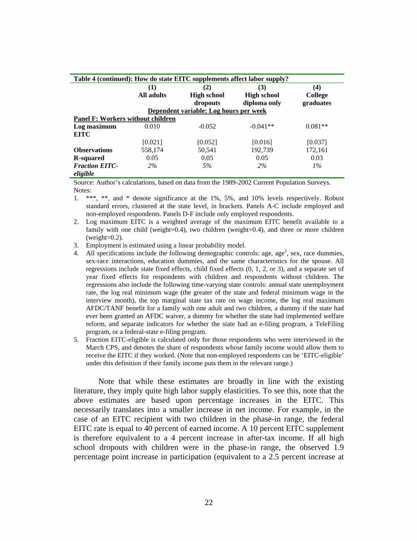
Note that while these estimates are broadly in line with the existing

literature, they imply quite high labor supply elasticities. To see this, note that the above estimates are based upon percentage increases in the EITC. This necessarily translates into a smaller increase in net income. For example, in the case of an EITC recipient with two children in the phase-in range, the federal EITC rate is equal to 40 percent of earned income. A 10 percent EITC supplement is therefore equivalent to a 4 percent increase in after-tax income. If all high school dropouts with children were in the phase-in range, the observed 1.9 percentage point increase in participation (equivalent to a 2.5 percent increase at

23

the mean) would imply a participation elasticity with respect to net income of 0.6. Since many high school dropouts with children are not in the phase-in range, 0.6 must be a lower bound for the true participation elasticity. Such a large elasticity implies that state EITCs led to a substantial increase in the labor supply of low-skilled workers, which is important to bear in mind when considering the effect on hourly wages. 4.3 State EITCs and hourly wages To determine the impact of changes in EITC generosity, I estimate a similar regression to equation (11), but with the dependent variable being the real pre-tax hourly wage w, which is deflated by the monthly CPI: ln(w)ist = α + βρst + δXist + πZst + ζs + λkt + εist (12)

Table 5 shows the result from estimating this equation. Across the entire adult workforce, a 10 percent increase in the generosity of the EITC is associated with a 1 percent fall in hourly wages – a substantial drop, given that only 9 percent of adult workers were eligible for the EITC. Across skill groups, raising the EITC is associated with a significant wage reduction for the low-skilled, but has no effect on high-skill wages, suggesting that the wage effect is due to the policy itself, rather than extraneous factors. The effect is large and significant: when the generosity of the EITC is increased by 10 percent, wages for high school dropouts fall by 5 percent, and wages for those with only a high school diploma fall by 2 percent. (Below, I discuss the possibility that these changes are driven by compositional shifts.)

Is the effect of the EITC to reduce wages to a larger extent for workers with children than childless workers? As has been demonstrated, the EITC is substantially more generous for employees with children, and the effect on labor force participation is significantly higher for this group. If workers with children are not close substitutes for childless workers, the wage effect of a boost in all EITC rates should be much more pronounced for parents than for childless employees. Alternatively, if parents and childless workers are close substitutes, one might expect that an increase in the generosity of the EITC will have the same effect on the wages of workers with and without children.

24

Table 5: How do state EITC supplements affect hourly wages? Dependent variable: Log real hourly wage (1) (2) (3) (4) All adults High school



graduates Panel A: With and without children Log maximum EITC

-0.121* -0.488*** -0.221*** 0.008


9% 25% 12% 3%

Panel B: With children Log maximum EITC

-0.156** -0.595*** -0.202** -0.048


18% 46% 23% 5%

Panel C: Without children Log maximum EITC

-0.092 -0.410*** -0.239*** 0.057


2% 5% 2% 1%

Source: Author’s calculations, based on data from the 1989-2002 Current Population Surveys. Notes: 1. ***, **, and * denote significance at the 1%, 5%, and 10% levels respectively. Robust standard

errors, clustered at the state level, in brackets. 2. Log maximum EITC is a weighted average of the maximum EITC benefit available to a family

with one child (weight=0.4), two children (weight=0.4), and three or more children (weight=0.2). 3. All specifications include the following demographic controls: age, age2, sex, race dummies, sex-

race interactions, education dummies, and the same characteristics for the spouse. All regressions include state fixed effects, child fixed effects (0, 1, 2, or 3), and a separate set of year fixed effects for respondents with children and respondents without children. The regressions also include the following time-varying state controls: annual state unemployment rate, the log real minimum wage (the greater of the state and federal minimum wage in the interview month), the top marginal state tax rate on wage income, the log real maximum AFDC/TANF benefit for a family with one adult and two children, a dummy if the state had ever been granted an AFDC waiver, a dummy for whether the state had implemented welfare reform, and separate indicators for whether the state had an e-filing program, a TeleFiling program, or a federal-state e-filing program.

4. Fraction EITC-eligible is calculated only for those respondents who were interviewed in the March CPS.

25

Panels B and C of Table 5 show the effect of increasing the generosity of the EITC on the hourly wages of workers with and without children. As the bottom row of each panel shows, the fraction of workers eligible for the EITC is much higher among those with children than those without. Yet for the two lowest skill groups, an EITC increase has a similar effect on the wages of workers with and without children. For high school dropouts, the wage drop associated with a 10 percent increase in the EITC is slightly greater for those with children (-6 percent) than for those without children (-4 percent). For those with only a high school diploma, the reduction in wages is approximately the same for those with and without children (-2 percent). This is quite consistent with standard models, which suggest that a negative income tax that induces a labor supply shock should affect all workers in that industry, not just those who receive the negative income tax.18

In Table 6, I present five robustness checks. Because state EITC supplements have been shown to be positively related to state GDP, Panel A includes a control for log state GDP per capita. Although the coefficient on state GDP is positive and significant in most specifications, the coefficient on the EITC remains very close to the preferred specification (Table 5, Panel A). Panel B of Table 6 estimates the results using only states that had an EITC at some point during the period 1989-2002, omitting states that never had an EITC. This has the advantage that the results are estimated only from differences in timing within the states that adopted an EITC at some point, and not from differences between EITC states and non-EITC states. Again, the coefficients in this specification are very close to those in the preferred specification.

In effect, the control group in the main specification is comprised of all states that never had an EITC, weighted in proportion to their population. Another approach is to give a higher weight to those states whose economies more closely tracked those of the EITC states in the period 1984-88 (when very few states had EITCs). This is done by employing the ‘synthetic control’ approach of Abadie and Gardeazabal (2003) and Abadie et al. (2007). Using data for 1984-88, I create a weighted set of ‘control states’ (the group of states that never had an EITC) with the weights being constructed so that the control states most closely approximate the treatment states (the states that had an EITC at some point in the period 1989-2002).19 For example, the synthetic control for Vermont is comprised of 29%

18 This fall in the equilibrium wage may have led to a drop in labor supply for ineligibles. Such an effect suggests that studies which use ineligibles as a control group may overestimate the treatment effect of the EITC. 19 This strategy is implemented using code available from Alberto Abadie’s website. For each of the 18 treatment states (those that ever had an EITC), I create a vector of weights using data for 1984-88, with the outcome variable being mean log hourly wages and predictor variables being

26

California and 71% Utah, while the synthetic control for Massachusetts is made up of 54% Connecticut, 28% Hawaii, and 18% New Hampshire. Simply pooling the control group (non-EITC states) effectively aggregates control states in proportion to state population. Under that approach, the control states that receive the most weight are California, Texas, and Florida. When the control states are aggregated using the synthetic control approach, the control states that receive the most weight are California, South Dakota, and Delaware. Panel C of Table 6 shows the results from this specification, which demonstrates that using the synthetic control approach makes virtually no difference to the results.

Another potential concern is that in some states, EITC supplements were non-refundable, which would likely have had less impact on labor supply (and therefore on wages) than refundable EITC supplements. In Panel D of Table 6, I drop states with non-refundable EITCs. Doing this has very little impact on the results. The final robustness check in Table 6 is to use an alternative measure of EITC generosity: the maximum EITC benefit for a family with one child. In Panel E, this is used in place of the weighted EITC measure. Once again, the coefficients and statistical significance remain very close to the preferred specification (Panel A of Table 5).20 log per-capita state GDP, the annual state unemployment rate, the log real minimum wage, the top marginal state tax rate on wage income, and the log real maximum AFDC/TANF benefit for a family with one adult and two children. Each vector of weights for a treatment state denotes the set of control states (those that never had an EITC) that most closely match the treatment state’s economic performance in 1984-88. These 18 vectors of weights for the treatment states are then combined into a single vector of weights by aggregating them in proportion to the population in each treatment state. Thus a control state receives a higher weight (a) the more closely its economy tracked that of a treatment state in 1984-88, and (b) the larger the population of the treatment state that it tracked. For example, the control state of Utah receives the highest weight when creating a set of synthetic controls for the treatment state of Maine. But when the weights are aggregated up, all the weights for smaller treatment states like Maine receive less weight than those for larger treatment states like New York. Standard errors are bootstrapped by randomly varying the weights given to the predictor variables in the pre-intervention period. I am grateful to Caroline Hoxby for suggesting this approach. 20 In Leigh (2004), I carry out two further robustness checks. First, I control for EITC generosity in the current and past year (accounting for the possibility that wages are sticky, or employees are slow to perceive the credit), and find that there is no lag between the EITC increase and the real wage fall (Figure 6 also provides visual confirmation of this). Second, I interact EITC generosity with the minimum wage (to account for the possibility that minimum wages act as a floor on the wage effect), and find that minimum wages have little impact on the incidence of the credit.

27

Table 6: State EITC supplements and hourly wages – robustness checks Dependent variable: Log real hourly wage Sample is workers with and without children (1) (2) (3) (4) All adults High school



graduates Panel A: Controlling for state GDP Log maximum EITC

-0.121** -0.481*** -0.217*** 0.006

[0.048] [0.122] [0.062] [0.039] Log state GDP per capita

0.273*** 0.168 0.265*** 0.312***

[0.052] [0.130] [0.060] [0.036] Observations 1,043,708 94,899 364,098 313,606 R-squared 0.32 0.2 0.19 0.15 Panel B: Omitting states that never had an EITC Log maximum EITC

-0.155* -0.417** -0.275*** -0.045

[0.078] [0.169] [0.085] [0.075] Observations 348,537 26,585 117,494 118,994 R-squared 0.30 0.18 0.17 0.14 Panel C: Synthetic control approach Log maximum EITC -0.102 -0.451*** -0.211** 0.018 [0.069] [0.147] [0.083] [0.055] Observations 1,043,708 94,899 364,098 313,606 R-squared 0.32 0.19 0.17 0.13 Panel D: Omitting states with non-refundable EITCs Log maximum EITC

-0.119* -0.474*** -0.221*** 0.002

[0.065] [0.136] [0.077] [0.058] Observations 993,303 91,209 347,763 296,996 R-squared 0.32 0.2 0.19 0.14 Panel E: Using maximum one-child EITC as the measure of EITC generosity Log maximum EITC

-0.120* -0.504*** -0.220*** 0.011

[0.066] [0.126] [0.076] [0.058] Observations 1,043,708 94,899 364,098 313,606 R-squared 0.32 0.2 0.19 0.14


standard errors, clustered at the state level, in brackets. 2. In Panels A to D, log maximum EITC is a weighted average of the maximum EITC benefit

available to a family with one child (weight=0.4), two children (weight=0.4), and three or more children (weight=0.2). In Panel E, log maximum EITC is the maximum EITC benefit available to a family with one child.

3. All specifications include the following demographic controls: age, age2, sex, race dummies, sex-race interactions, education dummies, and the same characteristics for the spouse. All

28

regressions include state fixed effects, child fixed effects (0, 1, 2, or 3), and a separate set of year fixed effects for respondents with children and respondents without children. The regressions also include the following time-varying state controls: annual state unemployment rate, the log real minimum wage (the greater of the state and federal minimum wage in the interview month), the top marginal state tax rate on wage income, the log real maximum AFDC/TANF benefit for a family with one adult and two children, a dummy if the state had ever been granted an AFDC waiver, a dummy for whether the state had implemented welfare reform, and separate indicators for whether the state had an e-filing program, a TeleFiling program, or a federal-state e-filing program.

4. The synthetic control approach follows Abadie and Gardeazabal (2003) and Abadie et al. (2007). For each of the 18 treatment states (those that ever had an EITC), I create a vector of weights using data for 1984-88, with the outcome variable being mean log hourly wages, and predictor variables being log per-capita state GDP, the annual state unemployment rate, the log real minimum wage, the top marginal state tax rate on wage income, and the log real maximum AFDC/TANF benefit for a family with one adult and two children. Each vector of weights for a treatment state denotes the set of control states (those that never had an EITC) that most closely match the treatment state’s economic performance in 1984-88. These 18 vectors of weights for the treatment states are then combined into a single vector of weights by aggregating them in proportion to the population in each treatment state. For all control state observations, these ‘synthetic control weights’ are then multiplied by the regular CPS population weights.

While it is difficult to precisely estimate the above effects in dollar terms,

these results suggest that the wage fall probably exceeds the full value of the credit. Recalling that the federal EITC is never higher than 40 percent, a 10 percent increase in the EITC cannot be worth more than 4 percent of the pre-tax wage. So if a 10 percent increase in the EITC leads to a 5 percent fall in pre-tax wages, the worker’s after-tax hourly wage will not rise as a result of the EITC. In the case of poor households with children, Neumark and Wascher (2001) found that state EITCs were associated with a rise in gross income for households with children: suggesting that the increase in labor supply offset the fall in wages. However, it is quite possible that poor households without children saw a fall in their gross income, since the EITC did not increase their labor supply, but nonetheless reduced their hourly wages.

Is this result consistent with standard labor demand elasticities? One way to check this is to compare the estimated labor supply effects (Table 4) and wage effects (Table 5). For simplicity, I focus only on the extensive margin, ignoring the impact of the EITC on hours worked. Recall from Panel A of Table 4 that a 10 percent increase in the EITC boosted participation of high school dropouts by 0.9 percentage points (1.5 percent at the mean participation rate), while in Panel A of Table 5, the same 10 percent increase in the EITC caused hourly wages of high school dropouts to fall by 5 percent. Using the formula dW/W=(dLS/LS)/ηD, this implies a labor demand elasticity of -0.3, which is consistent with estimates from aggregate studies, slightly above the standard estimates in the minimum wage literature, and below estimates from the immigration literature.

29

Note that while I have described this hourly wage impact as large, it would be larger still if the labor demand elasticity was closer to zero. For example, a labor demand elasticity of -0.1 implies that a 1.5 percent increase in labor supply would lead to a 15 percent fall in hourly wages. Viewed in this light, the hourly wage effect observed here is lower than many labor demand elasticities from the minimum wage literature would lead us to expect. The observed hourly wage effects should not be at all surprising, given the large labor supply effects induced by the EITC. 4.4 How might compositional changes affect these estimates? One concern with the above hourly wage estimates is that the fall in average wages may reflect a change in the composition of the workforce, rather than a fall in wages for existing workers. For example, if those induced to enter the workforce by an increase in the EITC are less able than the average employee with the same level of education, they would most likely be paid less than the average for an employee of their education level. An increase in the EITC would therefore cause the mean wage to fall, but without affecting those who were already in the workforce.

The most straightforward way to see that compositional changes are not driving the wage effects is to compare the effect of an EITC increase on workers with children (whose labor supply increased significantly), and workers without children (whose labor supply did not increase very much). Were the effect purely a compositional one, the wage effect would be much larger for workers with children. Yet as can be seen from a comparison of Panels B and C of Table 5, the wage effect is quite similar for both groups.

Another way to estimate the extent of the compositional effect is to carry out a bounds analysis (Manski 1995), assuming that all those who were induced by the EITC to enter the labor market earned precisely the minimum wage. As above, recall from Table 4 that a 10 percent increase in the EITC boosted participation of high school dropouts by 0.9 percentage points, or 1.5 percent at the mean participation rate (again, I ignore the impact on hours worked). In states that had an EITC supplement at any point during the interval 1989-2002, the minimum wage was 53 percent of the mean wage for high school dropouts. If all new entrants earned only the minimum wage, this would have lowered the average wage of dropouts by approximately 0.8 percent (0.53×0.015). By contrast, the estimates in Table 5 suggest that the overall impact of a 10 percent increase in the EITC was to cause hourly wages of high school dropouts to fall by 5 percent. Thus compositional changes can explain at most one-sixth of the total wage drop.

30

Intuitively, it should make sense that the compositional effects can account for only a small share of the overall impact. The compositional effect of adding another x percent of new workers who earn half the average wage will be to reduce the mean wage by approximately 0.5x. But the effect of moving down the labor demand curve will be to reduce the mean wage by x/ηD. For the compositional effect to dominate the labor demand effect, it would have to be the case that ηD<-2, which is below the estimates of the labor demand elasticity that have been found in aggregate studies and in the minimum wage literature.

Finally, it is worth noting that one channel through which compositional effects might operate is interstate migration. Given that overall compositional impacts are small, the portion due to interstate migration must be smaller still. This is consistent with most studies of welfare migration, which find small or zero effects of benefit generosity on migration decisions (see the review in Brueckner, 2000, and Cushing-Daniels, 2004). The assumption of states as self-contained labor markets appears reasonable, at least for the purpose of analyzing the effect of the EITC. 5. Using variation in the federal EITC across demographic groups While exploiting state variation in the EITC has certain advantages, it is useful to see whether the effects are qualitatively similar using an entirely different source of variation. In this section, I focus only on variation in the federal EITC, testing how wages are affected by the average federal EITC parameters in an employee’s gender-age-education cell (which I refer to as a ‘demographic group’). In the previous section, exploiting state variation in EITC rates, I assumed that states can be regarded as distinct labor markets. By contrast, this strategy assumes that demographic groups can be regarded as separate labor markets. To the extent that this assumption does not hold – in other words that labor supply is elastic across demographic groups – this will attenuate the estimated effects of the EITC. (For example, if employers cannot substitute a male high school graduate aged 30-34 for a female high school dropout aged 25-29, then the labor supply across these two groups can be regarded as inelastic. Conversely, if the two groups are perfect substitutes, labor supply across them is perfectly elastic.)

In using the share of people in a demographic group who are eligible for the federal EITC, my approach also differs from standard tax incidence models, which use the individual’s own tax parameters. The theoretical model in section 3 supports such an approach: a negative income tax that induces a rise in labor supply should reduce equilibrium wages for both eligibles and ineligibles. Merely applying a standard tax incidence model would not capture the effect of the EITC on the wage of ineligibles.

31

To define an individual’s demographic group, I assume that employees’ wages depend upon their gender, age and education. Dividing the adult population into 2 gender groups, 6 five-year age groups and 4 education groups, I construct a total of 48 gender-age-education groupings (see Data Appendix for details).21 In each case, I assume that labor supply is inelastic across demographic groups. In the previous section, the sample covered 1989-2002 (since few states had EITCs prior to 1989). Here, I extend the sample slightly to span 1984-2002, which has the advantage of taking into account the increase in the EITC that was part of the Tax Reform Act of 1986.

Since the actual share of people in a demographic group who are EITC-eligible is endogenous with respect to labor supply, it is necessary to create a measure that captures exogenous variation in the federal EITC. I therefore construct a simulated instrument for the EITC rate (in the spirit of Currie and Gruber 1996). To estimate the share of people in a demographic group eligible for the federal EITC, I use the 1 percent sample of the 1990 census to calculate precise measures of family structure and income distribution (by centile) within each demographic group. For each of the years 1984-2002, I calculate the actual earnings of taxpayers at the 1st centile, 2nd centile, and so on, using the March CPS. Holding constant the family structure and income distribution within each demographic group, I can then assign a dollar income to each type of family in each demographic group. Using the National Bureau of Economic Research’s Taxsim program, I then calculate for each demographic group and year the fraction of EITC-eligible employees (see Data Appendix for details). These tax rates are a simulated instrument for the actual share of EITC-eligible employees within a given demographic group.

For example, given the income and family composition of 25-29 year old female high school dropouts in the 1990 census, the simulated instrument implies that the federal EITC expansion of the 1990s would have led the share of 25-29 year old female high school dropouts receiving the EITC to grow from 27 percent in 1984 to 50 percent in 2002. Similarly, given the income and family composition of 45-49 year old male college graduates in the 1990 census, the simulated instrument implies that the share of 45-49 year old male college graduates receiving the EITC should have risen from 1 percent in 1984 to 4 percent in 2002. These changes are identified from the interaction between federal EITC parameters and the characteristics of the demographic group in 1990.

There are a number of benefits to adopting such an approach. First, it accords with the theoretical model in section 3 and with the findings from variation in state EITC supplements in section 4. Second, using the census 1

21 The results are not especially sensitive to these particular gender-age-education groupings.

32

percent sample to determine family structure and income distribution within a demographic group provides much more precise measures than the CPS. Third, using a different dataset to construct the simulated instrument eliminates the possibility of correlation between the error in the wage equation and in the tax rate. And fourth, by using average EITC parameters rather than the individual’s own parameters, I need not assume – as most of the previous literature has done – that an employee’s marital status and number of children is exogenous with respect to the generosity of the EITC.22

In what follows, I focus on the share of people in a given demographic group who are EITC-eligible (results for the average and marginal EITC rates are set out in Leigh 2004). As in the previous section of the paper, I first test whether increasing the share of workers in a demographic group who are eligible for the EITC has an effect on employment or hours worked, and then whether it has an impact on hourly wages. Formally, I estimate the following regressions: LSjt = α + β(%EITC)jt + θj + λt + εjt (13) ln(W)jt = α + β(%EITC)jt + θj + λt + εjt (14)

where LS is a measure of the average labor supply in demographic group j in year t, W is average log real hourly wages, %EITC is a simulated instrument for the fraction eligible in a demographic group, θ is a fixed effect for the employee’s demographic group (i.e. their gender-age-education cell), and λ is a vector of year fixed effects. Results are estimated at the demographic group × year level (but are similar if estimated at the individual level). I estimate both a reduced-form regression, in which the key independent variable is the predicted fraction eligible (using the simulated instrument), and an instrumental variable regression, in which the actual share who are EITC-eligible is instrumented with the predicted share.

22 Ellwood (2000) finds only minimal effects of the EITC on marriage rates, but some impact on cohabitation patterns, suggesting that the impact of the EITC on family structure might have become more apparent since then. Baughman and Dickert-Conlin (2003) estimate that a 10 percentage point increase in the maximum EITC benefit increases the probability of non-white women having a first child or an additional child by 0.3 percent, while having no effect on the childbearing decisions of white women.

33

Table 7: Using federal EITC variation across gender-age-education cells (1)

Reduced Form (2) IV

Panel A: Dependent variable is share employed Predicted share EITC-eligible 0.016 [0.088] Actual share EITC-eligible 0.019 [0.105] Observations 912 912 R-squared 0.98 0.97 Panel B: Dependent variable is average log hours worked per week Predicted share EITC-eligible 0.035 [0.046] Actual share EITC-eligible 0.043 [0.056] Observations 912 912 R-squared 0.97 0.97 Panel C: Dependent variable is average log real hourly wage Predicted share EITC-eligible -0.853*** [0.158] Actual share EITC-eligible -1.037*** [0.198] Observations 912 912 R-squared 0.99 0.98


standard errors in brackets. Standard errors are clustered at the gender-age-education cell level.

2. Predicted share EITC-eligible is based upon taking the income and family type distribution in a given gender-age-education cell in the 1990 census, and applying it to the tax parameters in a given year. See Data Appendix for details.

3. IV specification instruments the actual share EITC-eligible with the predicted share EITC-eligible. The first-stage regression is identical in each stage, with an F-test on the excluded instrument of 137.50 (P<0.01) and a partial R-squared on the excluded instrument of 0.33. The R-squared reported for the IV specifications is the centred R-squared on the second-stage regression.

4. All specifications are estimated using data aggregated to the gender-age-education cell × year level, and include gender-age-education cell fixed effects and year fixed effects.

Table 7 shows the results of these regressions. Where the dependent

variable is employment (Panel A), this specification indicates that a 10 percentage point rise in the share of workers in a demographic group that are EITC-eligible increases participation by 0.2 percentage points, but the effect is not statistically significant in either the reduced form or IV specification. In Panel B, I use log hours as the dependent variable, and find a positive impact of EITC eligibility on hours worked, but the effect is again not statistically significant. Across gender-

34

age-education groups, a 10 percentage point increase in share EITC-eligible leads to a statistically insignificant 0.4 percent rise in hours worked. Panel C uses log hourly wages as the dependent variable. In this specification, a 10 percentage point increase in the share of EITC-eligible workers leads to a statistically significant 9 percent fall in hourly wages in the reduced form specification, and a 10 percent wage fall in the IV specification. This is shown graphically in Figure 7, which plots the change from 1984-85 to 2001-02. In general, the results from these specifications are consistent with the (more precisely estimated) results from the previous section: a rise in the EITC increases labor supply, which in turn leads to a reduction in hourly wages.23

23 Note that the measure of EITC generosity differs in the state specification (section 4) and the federal specification (section 5). The state specification uses as the key independent variable the maximum EITC payment in a state and year, while the federal specification uses as the key independent variable the share in a demographic group who are EITC-eligible in a given year. Both approaches allow for spillover effects on ineligible coworkers, but because the two measures differ, it is difficult to compare magnitudes. One way to reconcile these results is to estimate a regression using state data, but with the key independent variable being the share of workers in a state who are EITC-eligible, instrumented using the maximum EITC payment (and including the same control variables as in Table 5). With log hourly wages as the dependent variable, the coefficient on the share eligible is -1.7, which is statistically significant at the 5 percent level. This is broadly consistent with the corresponding IV specification in Table 7 (a coefficient of -1.0), but suggests that labor supply is more elastic across demographic groups than across state boundaries (as one might expect).

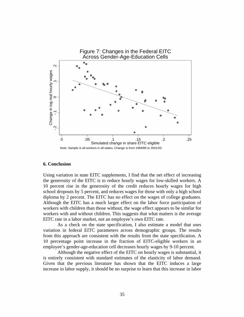
35

-.2-.1

0.1

.2C

hang

e in

log

real

hou

rly w

ages

0 .05 .1 .15 .2 .25Simulated change in share EITC eligible

Note: Sample is all workers in all states. Change is from 1984/85 to 2001/02.

Figure 7: Changes in the Federal EITCAcross Gender-Age-Education Cells

6. Conclusion Using variation in state EITC supplements, I find that the net effect of increasing the generosity of the EITC is to reduce hourly wages for low-skilled workers. A 10 percent rise in the generosity of the credit reduces hourly wages for high school dropouts by 5 percent, and reduces wages for those with only a high school diploma by 2 percent. The EITC has no effect on the wages of college graduates. Although the EITC has a much larger effect on the labor force participation of workers with children than those without, the wage effect appears to be similar for workers with and without children. This suggests that what matters is the average EITC rate in a labor market, not an employee’s own EITC rate.

As a check on the state specification, I also estimate a model that uses variation in federal EITC parameters across demographic groups. The results from this approach are consistent with the results from the state specification. A 10 percentage point increase in the fraction of EITC-eligible workers in an employee’s gender-age-education cell decreases hourly wages by 9-10 percent.

Although the negative effect of the EITC on hourly wages is substantial, it is entirely consistent with standard estimates of the elasticity of labor demand. Given that the previous literature has shown that the EITC induces a large increase in labor supply, it should be no surprise to learn that this increase in labor

36

supply has the effect of reducing hourly wages. As other researchers have shown, boosting the EITC increases the gross income of poor families with children, reflecting the fact that the rise in labor supply more than offsets the fall in hourly wages.

A clear implication of this paper is that the EITC may harm low-skilled workers who are ineligible for the EITC (or receive only a small credit). Because those with and without children will generally be paid the same equilibrium wage, high school dropouts without children probably experience a reduction in their after-tax earnings when the EITC increases. The indirect burden that the EITC imposes on low-income childless adults deserves greater consideration by policymakers. Data Appendix Real hourly wages: To obtain the largest possible cross-section of workers, I use the Current Population Survey Merged Outgoing Rotation Group (CPS MORG), which contains precise data on hourly earnings and comprises around 30,000 individuals per month. For employees paid on an hourly basis, the wage is directly reported. For other workers, hourly earnings are calculated by dividing weekly earnings by usual weekly hours. The sample is restricted to those in the labor force aged 25-55 (workers nearing retirement age sometimes report anomalous earnings). Self-employed workers are excluded, since their hourly earnings are unreliable. Extreme wage observations – those in which employees reported earning less than half the federal minimum wage, or more than 100 times the federal minimum wage – are excluded. Wages are converted into 2002 dollars using the monthly CPI. Children: From 1984 onwards, it is possible to determine the respondent’s family type and number of children from the CPS. From 1984-1993, and from November 1999-2002, the number of children is drawn from the MORG sample. Unfortunately, from January 1994 until October 1999, the basic monthly CPS (from which the MORG sample is drawn) did not ask respondents for their number of children. For this period, therefore, the MORG records for January 1994 to October 1999 were merged with the March CPS records for the same years (no other supplementary surveys included this question), resulting in a successful merge rate of around 80 percent. Note that the March survey is used only for the purpose of determining the respondent’s number of children – hourly earnings are still derived from the MORG file. Sample weights are adjusted so that the years 1994-1999 are not under-weighted in the regressions.

37

EITC parameters: Federal EITC parameters from Internal Revenue Service, Individual Income Tax Return (form 1040), various years. State EITC supplements for early years from Neumark and Wascher (2001), and for recent years from Nicholas Johnson of the Center on Budget and Policy Priorities. Real State GDP per capita: From Bureau of Economic Analysis, Regional Economic Accounts (http://www.bea.gov/). Converted to current dollars using the annual national CPI. State unemployment rate: From Bureau of Labor Statistics, Local Area Unemployment Statistics (www.bls.gov/data/). Real minimum wage: The greater of the state and federal minimum wage then prevailing, converted into 2002 dollars using the annual national CPI. Data supplied by Raj Chetty and Jesse Shapiro. State tax rate: The top marginal state tax rate on income earned from wages, from the NBER’s Taxsim related files page (www.nber.org/~taxsim). Real maximum welfare benefit: The maximum AFDC/TANF benefit available for a family of three (one adult and two children) with no income, as at December of that year, converted into 2002 dollars using the annual CPI. In states where benefits vary by region, the figure is for the region with the largest caseload. Figures for Hawaii are for families on welfare for more than two months (a more generous benefit is initially available). Figures for New Mexico do not include housing subsidy. Figures for Wisconsin are for families not headed by a disabled adult. Figures for Nevada are for families without foster children. Data for 1989-1998 supplied by Adam Looney, and figures for 1999-2002 from annual TANF reports, produced by the Department of Health and Human Services, Office of Family Assistance (www.acf.hhs.gov/programs/ofa/indexar.htm). Welfare reform: A dummy indicating whether the state had implemented TANF by the end of that year. It equals 0 for all states in 1989-95, and 1 for all states from 1998-2002. Data for all years from Adam Looney. Aid for Dependent Children program waiver: A dummy indicating whether the state had ever received an AFDC waiver (as at the end of that year). No states received waivers prior to 1992. Since AFDC has now been abolished, states are coded with the same value in 1998-2002 as they had in 1997. Data for all years from Adam Looney.

38

State Electronic Filing Program: A dummy indicating whether the state had introduced an electronic filing program, sourced from Kopczuk and Pop-Eleches (2007). State TeleFiling Program: A dummy indicating whether the state had introduced a program allowing taxpayers to file by telephone, sourced from Kopczuk and Pop-Eleches (2007). Federal-State Electronic Filing Program: A dummy indicating whether the state was part of the federal-state electronic filing program, sourced from Kopczuk and Pop-Eleches (2007). Variation in the federal EITC across demographic groups: I construct 48 gender-age-education groups, collapsing the sample into 2 genders, 6 age groups (25-29, 30-34, 35-39, 40-44, 45-49, 50-55), and 4 education groups (high school dropouts with 11 or fewer years of schooling, high school graduates with exactly 12 years of schooling, some college with 13-15 years of schooling, and college graduates with 16 or more years of schooling). The procedure for calculating EITC parameters for each gender-age-education cell (‘demographic group’) is as follows. First, I take all employed adults (aged 25-55) from the 1990 census 1 percent sample (Ruggles et al. 2008). Across all adults in the sample, I calculate an overall income distribution and assign each person to an income centile (1 to 100), based on their family income. Next, for each demographic group, I calculate the fraction of people in six family types – married with 0, 1, or 2+ children, and single with 0, 1, or 2+ children. For each family type within each demographic group, I then calculate the fraction of employees at each income centile. For each demographic group, I now have 606 parameters – the full centile income distribution for each of the six family types, and a single number denoting the share of each family type in that demographic group. To apply the EITC parameters to the prevailing tax rules, it is necessary to know the national income distribution in a given year. To determine this, I use the family income distribution among adults aged 25-55, as reported in the following year’s March CPS (since the March CPS asks about earnings in the previous year). Combining this data with the demographic group-level family and income distribution from the 1990 census, I assign earnings to each centile. This information is then entered into the NBER Taxsim program, which calculates the relevant tax parameters. I assume that all family income is wage earnings, that there are no other government transfers, and that married couples file jointly. The resulting tax parameters are then averaged up by demographic group, weighted by the share of each centile and family type.

39

Appendix Table 1: Summary Statistics for State EITC Specifications Mean SD N Main variables Employed 0.781 0.413 1376795 Log hours 3.662 0.307 1048490 Log real hourly wage 2.769 0.541 1043708 Log maximum EITC 0.018 0.278 1376795 State controls Log state GDP per capita 10.397 0.164 1376795 Unemployment rate 0.057 0.015 1376795 Log real minimum wage 1.678 0.074 1376795 Maximum AFDC benefit 6.100 0.436 1376795 Welfare reform 0.423 0.494 1376795 AFDC waiver 0.396 0.489 1376795 Top marginal state tax rate 0.052 0.032 1376795 State electronic filing program 0.487 0.500 1376795 State TeleFiling program 0.254 0.436 1376795 Federal-State electronic filing program 0.361 0.480 1376795 Individual controls Male 0.484 0.500 1376795 Age 38.819 8.549 1376795 Black 0.119 0.324 1376795 Hispanic 0.092 0.289 1376795 Other non-white 0.043 0.203 1376795 High school dropout 0.129 0.335 1376795 High school only 0.347 0.476 1376795 College educated 0.272 0.445 1376795 Number of children 0.856 1.052 1376795 Married 0.685 0.464 1376795 Note: Sample covers 1989-2002, including all adults aged 25-55 and not self-employed with non-missing covariates (as used in Table 4, Panel A, Column 1). Specifications where the dependent variable is log hours or hourly wages are restricted to those in employment. See Data Appendix for variable definitions. Appendix Table 2: Summary Statistics for Federal EITC Specifications Mean SD N Employed 0.757 0.150 912 Log hours 3.647 0.091 912 Log real hourly wage 2.691 0.321 912 Share EITC-eligible in demographic group 0.150 0.119 912 Note: Sample covers 1984-2002, including all adults aged 25-55 and not self-employed with non-missing covariates. Data are aggregated to the gender-age-education cell × year level. See Data Appendix for variable definitions.

40

References Abadie, A. and J. Gardeazabal. 2003. “Economic Costs of Conflict: A Case

Study of the Basque Country”, American Economic Review 93(1): 113-132. Abadie, A., A. Diamond, and J. Hainmueller. 2007. “Synthetic Control Methods

for Comparative Case Studies: Estimating the Effect of California's Tobacco Control Program”, NBER Technical Working Paper No. 335, Cambridge, MA: NBER.

Azmat, G. 2006. “The Incidence of an Earned Income Tax Credit: Evaluating the

Impact on Wages in the UK”, CEP Discussion Paper 724, Centre for Economic Performance, London School of Economics and Political Science, London, UK.

Baughman, R. and S. Dickert-Conlin. 2003. “Did Expanding the EITC Promote

Motherhood?”, American Economic Review 93(2): 247-251. Bertrand, M., E. Duflo, and S. Mullainathan. 2004. “How Much Should We Trust

Differences-in-Differences Estimates?”, Quarterly Journal of Economics 119(1): 249-275.

Bewley, T. 2004. “Fairness, Reciprocity, and Wage Rigidity”, IZA Discussion Paper 1137, Bonn: IZA.

Bingley, P. and G. Lanot. 2002. “The Incidence of Income Tax on Wages and Labour Supply”, Journal of Public Economics 83(2): 173-194.

Borjas, G. 2003. “The labor demand curve is downward sloping: reexamining the impact of immigration on the labor market”, Quarterly Journal of Economics 118(4): 1335-1374.

Brown, C., C. Gilroy, and A. Kohen. 1982. “The Effect of the Minimum Wage on Employment and Unemployment”, Journal of Economic Literature 20(2): 487-528.

Brueckner, J. 2000. “Welfare Reform and the Race to the Bottom: Theory and Evidence”, Southern Economic Journal 66: 505-525.

Currie, J. and J. Gruber. 1996. “Health insurance eligibility, utilization of medical care, and child health”, Quarterly Journal of Economics 111(2): 431-466.

41

Cushing-Daniels, B. 2004. “Migration in the US: What Role Welfare?”, mimeo, Gettysburg, PA: Gettysburg College.

Di Nardo, J., N. Fortin, and T. Lemieux. 1996. “Labor Market Institutions and the Distribution of Wages, 1973-1992: A Semiparametric Approach”, Econometrica 64(5): 1001-1044.

Eissa, N. and H. Hoynes. 2004. “Taxes and the Labor Market Participation of

Married Couples: The Earned Income Tax Credit”, Journal of Public Economics 88(9-10): 1931-1958.

Eissa, N. and H. Hoynes. 2006. “Behavioral Responses to Taxes: Lessons from

the EITC and Labor Supply”, in J. Poterba (ed.), Tax Policy and the Economy. Vol. 20, Cambridge, MA: MIT Press, 74-110.

Eissa, N. and J. Liebman. 1996. “Labor Supply Response to the Earned Income

Tax Credit”, Quarterly Journal of Economics 111(2): 605-637. Ellwood, D. 2000. “The Impact of the Earned Income Tax Credit and Social

Policy Reforms on Work, Marriage, and Living Arrangements”, National Tax Journal 53: 1063-1106.

Fullerton, D. and G. Metcalf. 2002. “Tax Incidence”, in A.J. Auerbach and M.

Feldstein (eds.), Handbook of Public Economics. Vol. 4, Oxford: Elsevier, 1787-1872.

Gourio, F. and P. Noual. 2006. “The Marginal Worker and the Aggregate Elasticity of Labor Supply”, mimeo, Boston, MA: Boston University.

Gruber, J. 1994. “The Incidence of Mandated Maternity Benefits”, American Economic Review 84(3): 622-641.

Gruber, J. 1997. “The Incidence of Payroll Taxation: Evidence from Chile”, Journal of Labor Economics 15(3, Pt 2), S72-S101.

Gruber, J. and A. Krueger. 1991. “The Incidence of Mandated Employer-Provided Insurance: Lessons from Workers’ Compensation Insurance”, in D. Bradford (ed.), Tax Policy and the Economy 5. Cambridge, MA: MIT Press, 111-143.

42

Hamermesh, D.S. 1987. “The demand for labor in the long run”, in O. Ashenfelter and R. Layard (eds.), Handbook of Labor Economics. Vol. 1, New York: North Holland/Elsevier, 429-471.

Hoffman, S. and L. Seidman. 2002. Helping Working Families: The Earned Income Tax Credit. Washington, DC: W.E. Upjohn Institute.

Hotz, V. and J. Scholz. 2003. “The Earned Income Tax Credit”, in R. Moffitt (ed.), Means-Tested Transfer Programs in the United States. Chicago, IL: University of Chicago Press, chapter 3.

Johnson, N. 2001. A Hand Up: How State Earned Income Tax Credits Help Working Families Escape Poverty in 2001. Washington, DC: Center on Budget and Policy Priorities.

Kopczuk, W. and K. Pop-Eleches. 2007. “Electronic Filing, Tax Preparers and Participation in the Earned Income Tax Credit”, Journal of Public Economics 91(7-8): 1351-1367.

Kubik, J. 2004. “The Incidence of Personal Income Taxation: Evidence from the Tax Reform Act of 1986”, Journal of Public Economics 88(7-8): 1567-1588.

Kuney, S. and J. Levitis. 2007. “How Much Would a State Earned Income Credit Cost in 2008?”, Washington, DC: Center on Budget and Policy Priorities, February 7.

Leigh, A. 2004. “Who Benefits from the Earned Income Tax Credit? Incidence Among Recipients, Coworkers and Firms”, Australian National University CEPR Discussion Paper 494, Canberra: ANU.

Longhi, S., P. Nijkamp, and J. Poot. 2005. “A Meta-Analytic Assessment of the Effect of Immigration on Wages”, Journal of Economic Surveys 19(3): 451-477.

Manski, C. 1995. Identification Problems in the Social Sciences. Cambridge, MA: Harvard University Press.

Meyer, B. 2002. “Labor Supply at the Extensive and Intensive Margins: The EITC, Welfare, and Hours Worked”, American Economic Review 92(2): 373-379.

43

Meyer, B. and D. Holtz-Eakin. (Eds.) 2002. Making Work Pay: The Earned Income Tax Credit and Its Impact on America's Families. New York, NY: Russell Sage Foundation.

Meyer, B. and D. Rosenbaum. 2001. “Welfare, the Earned Income Tax Credit, and the Labor Supply of Single Mothers”, Quarterly Journal of Economics 116: 1063-1114.

Neumark, D. and W. Wascher. 2001. “Using the EITC to Help Poor Families: New Evidence and a Comparison with the Minimum Wage”, National Tax Journal 54: 281-318.

Neumark, D. and W. Wascher. 2007. “Minimum Wages and Employment”, Foundations and Trends in Microeconomics 3(1-2): 1-182.

Romich, J. and T. Weisner. 2000. “How Families View and Use the EITC: Advance Payment versus Lump Sum Delivery”, National Tax Journal 53: 1245-1264.

Rothstein, J. 2008. “The Unintended Consequences of Encouraging Work: Tax Incidence and the EITC”, mimeo, Princeton, NJ: Princeton University.

Ruggles, S., M. Sobek, T. Alexander, C.A. Fitch, R. Goeken, P.K. Hall, M. King, and C. Ronnander. 2008. Integrated Public Use Microdata Series: Version 4.0 [Machine-readable database]. Minneapolis, MN: Minnesota Population Center. Available at http://usa.ipums.org/usa/

Summers, L. 1989. “Some Simple Economics of Mandated Benefits”, American Economic Review 79(2): 177-183.

United States Treasury. 2003. “Taxpayers Were Assessed Additional Tax for Advance Earned Income Credit Payments Not Received”, Publicly released memorandum. Ref No. 2003-40-126.

who benefits from the earned income tax credit? incidence among

Documents