Who Holds Cash? And Why?

Calvin Schnure”

January 1998

.

“ Economist, Federal Reserve Board. I am grateful to Jim Bohn, Craig Furfine, Jeff Marquardt,

Athanasios Orphanides and Karl Whelan for comments. The views expressed in this paper are those of theauthor and do not reflect the views of the Board of Governors or the staff of the Federal Resetve System. Email:schnurec@frb. gov.

Who Holds Cash? And Why?

The existing literature on investment and cash flow has tended to take the financialcharacteristics of firms as exogenously given, and then relate these characteristics to firminvestment behavior. We turn this approach on its head and take real characteristics of the

firm as given and examine patterns of cash holdings using firm-level data on nonfinancial firmsfrom COMPUSTAT. First we establish stylized facts about cash holdings, then investigate

possible motivations for firm behavior.

Cash holdings range widely, and are systematically related to firm size, industry andwhether or not the firm has borrowed in the public bond market. Cross-sectional regressionsindicate that cash holdings are positively correlated with proxies for agency problems,suggesting that firms that cannot borrow easily due to these agency problems hold greater cashstocks–perhaps as a cushion to prevent shortfalls in cash flow from impinging on investment.

While at first glance this may appear to support the argument that credit marketfrictions are responsible for the high correlation between cash flow and investment, the dataon cash holdings prove useful in focussing more closely on firms likely to become constrained.Previous research has identified firms without access to public bond markets as those mostlikely to face cash flow constraints; this group makes up about 85 percent of theCOMPUSTAT universe. However, cash holdings appear to be correlated with agencyproxies only for the very high cash holding firms, especially small firms. The group ofafflicted firms appears to be far smaller than suggested by other studies, less than one-quarterof the COMPUSTAT firms.

Introduction

Why do firms hold stocks of liquid assets? Firms that invest in cash (including bank

accounts) and securities while they have outstanding short-term debt incur a substantial cost,

as the spread between the interest they pay on their own borrowings and the rate they receive..

on investments can be quite large. This paper examines holdings of cash and securities (“cash”

for short) by nonfinancial firms. Previous research on the demand for liquid assets by

nonfinancial firms has been almost exclusively related to monetary aggregates, using aggregate

data to investigate money demand functions (see Barr and Cuthbertson (1992) for an example

and further references). In cent rast, we are concerned with cross-sectional variation in the

demand for liquid asset holdings by nonfinancial firms.

The literature on investment and cash flow has tended to take the financial

characteristics of firms as exogenously given, and then relate these characteristics to firm

investment behavior. We turn this approach on its head and take real characteristics of the

firm as given and examine patterns of cash holdings using firm-level data on nonfinancial firms

from COMI?USTAT. First we establish stylized facts about cash holdings, then investigate

possible motivations for firm behavior.

Cash holdings range widely, and are systematically related to firm size, industry, and

whether or not the firm has borrowed in the public bond market. Cross-sectional regression

analysis indicates that cash holdings are positively correlated with proxies for agency

problems, and suggests that firms that cannot borrow easily due to these agency problems

hold greater cash stocks--perhaps as a cushion to prevent shortfalls in cash flow from

impinging on investment.

This finding links this paper with the literature on the relationship between cash flow

and investment (for example, Fazzari, Hubbard and Petersen (1988); Hoshi, Kashyap and

Scharfstein (1991); Cummins, Hassett and Oliner (1997)). While at first glance our results

may appear to support the argument that credit market frictions are responsible for the high ‘--

correlation between cash flow and investment, the data on cash holdings prove useful in

focussing more closely on firms likely to become financially constrained. Some researchers

have identified firms without access to public bond markets as those most likely to face cash

flow constraints (Whited (1992); Gilchrist and Himmelberg (1995)); this group makes up

about 85 percent of the COMPUSTAT universe. However, the correlation between cash

holdings and agency proxies is driven by a subset of firms with very high cash holdings, which

exceed one quarter or even one half of the firm’s total assets. The group of afflicted firms

appears to be a far smaller subset of the total than suggested by previous research,

corresponding to between 10 and 25 percent of all COMPUSTAT firms.

This paper is organized as follows: the next section presents basic descriptive statistics

on cash holdings, and relates them to other characteristics of the firm, including size and

whether the firm has issued public bond debt. Section II develops a model of a firm’s choice

of cash holdings, given a (firm-specific) probability of being credit constrained at some date in

the future. Section III presents regression results of cash holdings of manufacturing firms.

Section IV concludes.

I. Who holds cash?

Table 1 presents the basic pattern of cash holdings among nonfinancial firms listed in

2

COMPUSTAT.l The vast majority of the firms in this sample are relatively small, with total

assets below $250 million. The median firm in this bottom size group holds cash equal to 10

percent of its total assets. The distribution of cash holdings has a huge upper tail, however:

the firm at the 90 percentile holds cash comprising 60 percent of total assets. These small

firms have relatively low leverage, with stockholders’ equity exceeding half of total assets for

the median firm.

Better access to credit markets, economies of scale in cash management, less volatile

cash flows and other factors contribute to a strong size effect in cash ratios. Cash stocks

relative to total assets decline for larger firms, falling to 4 percent for the median firm in the

$250 million to $500 million asset class, to as low as 2 percent or below for median firms in

the top size groups. The upper tail also diminishes as one moves to larger size groups. Cash

ratios at the 90th percentile drop sharply, to the 20 percent range for firms up to $1 billion in

assets, and around 10 percent for median firms in the largest size groups. However, the

distribution remains rather skewed even for the biggest firms, with firms at the 90th percentile

of the top size group having a cash ratio more than five times as large as that of the median

firm. Chart 1 graphs cash ratios for firms, by size deciles.

Cash holdings show a similar pattern when firms are grouped by bond rating, shown

in the lower panel of Table 1. Firms without a rating--which are mainly firms in the smaller

two size categories in the top panel--have relatively high cash ratios, 8 percent of assets at the

median and 55 percent at the 90th percentile. The median firm with debt rated below

Data are very similar if we restrict the sample to manufacturing firms only.

3

investment grade has a 4 percent ratio (I9 percent at the 90th percentile), while the median

investment grade firm has a 2 percent ratio (11 percent at the 90th percentile).

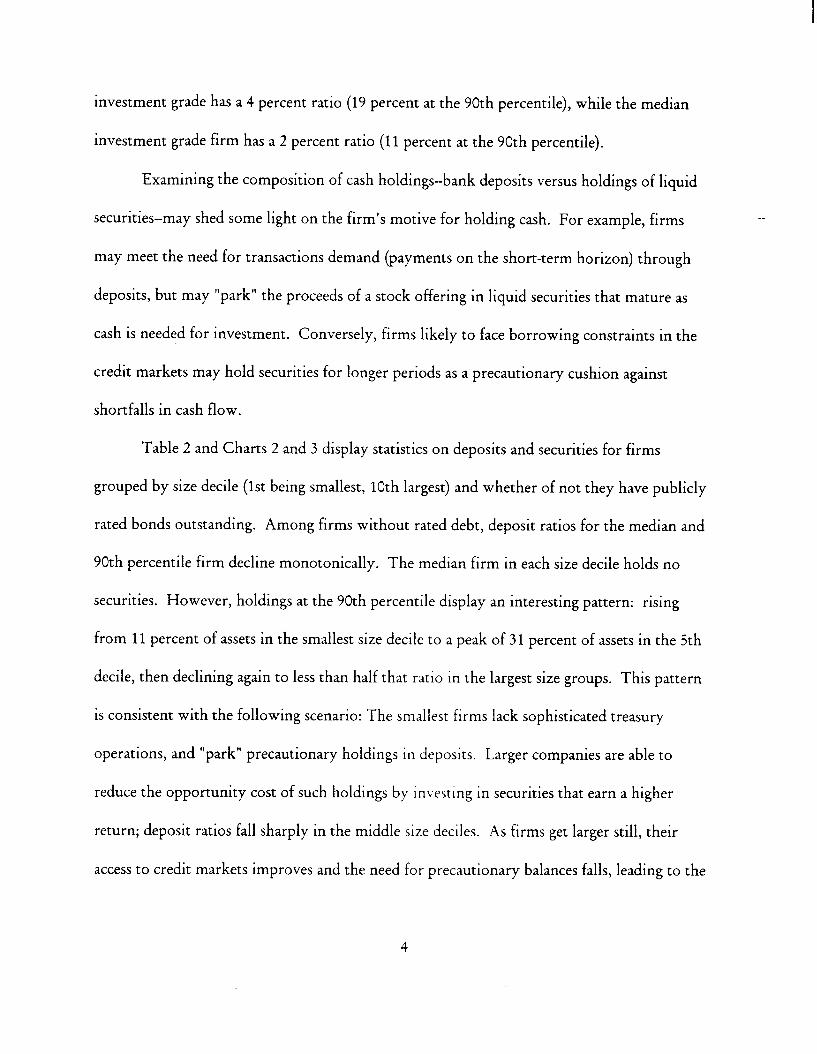
Examining the composition of cash holdings-bank deposits versus holdings of liquid

securities--may shed some light on the firm’s motive for holding cash. For example, firms

may meet the need for transactions demand (payments on the short-term horizon) through

deposits, but may “park” the proceeds of a stock offering in liquid securities that mature as

cash is needed for investment. Conversely, firms likely to face borrowing constraints in the

credit markets may hold securities for longer periods as a precautionary cushion against

shortfalls in cash flow.

Table 2 and Charts 2 and 3 display statistics on deposits and securities for firms

grouped by size decile (lst being smallest, IOth largest) and whether of not they have publicly

rated bonds outstanding. Among firms without rated debt, deposit ratios for the median and

90th percentile firm decline monotonically. The median firm in each size decile holds no

securities. However, holdings at the 90th percentile display an interesting pattern: rising

from 11 percent of assets in the smallest size decile to a peak of 31 percent of assets in the 5th

decile, then declining again to less than half that ratio in the largest size groups. This pattern

is consistent with the following scenario: The smallest firms lack sophisticated treasury

operations, and “park” precautionary holdings in deposits. Larger companies are able to

reduce the opportunist y cost of such holdings by investing in securities that earn a higher

return; deposit ratios fall sharply in the middle size deciles. As firms get larger still, their

access to credit markets improves and the need for precautionary balances falls, leading to the

drop in securities holdings relative to total assets.2

There are no firms with public debt ratings in the bottom half of the sample, and very

few in the 5th (4 firms) or 6th (I4 firms) size deciles (middle and bottom of Table 2, and

Charts 4 and S). The ratio of deposits to assets declines only slightly for median firms in

larger groups. Furthermore, firms with rated debt have far lower securities holdings relative

to total assets than do unrated firms. At the 90th percentile, these holdings are 5 percent of

assets or less (both investment grade and junk-rated firms), compared with doubledigit

holdings at the upper tail of unrated firms. This corroborates the observation that unrated

firms may use securities as a precautionary balance to insure against credit constraints that

may become binding in the future. Firms that have accessed public debt markets in the past

are less likely to face such constraints, and therefore have less need to hold securities.3

To explore one possible explanation of the upper tail of firms with very high cash

holdings, Table 3 shows stock issuance in the current and previous year’ as a percent of total

assets, for firms ranked by liquidity decile. In the groups of firms with low cash holdings,

very few had any stock issuance at all: in each of the bottom 6 groups, 75 percent or more of

z It is interesting to note that there are a number of firms (100) in the largest size

decile, with total assets greater than $1.5 billion, that do not have public debt outstanding.

3 The unusually large tail in Chart 5, deciles 5 and 6, results from there being very few

firms with public debt in these size categories. These may be firms that have recently issued

debt and are parking the proceeds in securities.

4 I examine two years of stock issuance because firms tend to maintain high cash

balances for a number of years after a major stock offering. Data for current-year issuanceonly show a similar pattern but lower totals; including more years has little effect on the data.

5

firms reported figures of 3 percent of total assets or less.s

Stock proceeds become a more important source of cash for those firms with large

holdings of liquid assets. Two-year issuance as a percentage of assets jumps in the final two

groups, to 15 and 52 percent, respectively, at the 75th percentile. Stock issuance appears to

account for a substantial fraction of firms with very liquid balance sheets. However, this

explains only a portion of the large upper tail of cash holdings, as these firms represent

perhaps five percent of the total sample (25 percent of the top liquidity decile equals 2.5

percent of the total sample). One possible explanation is that these are precautionary cash

balances held by firms that may face borrowing constraints if cash flow should faker. The

next section develops a simple model of a firm that chooses its level of cash holdings based on

the probability that it will be unable to borrow in the future.

II. A simple model of demand for cash holdings.

Let us consider a simple two-period model of a firm with an investment project, which

requires an investment at time t= 1; has uncertain cash flows at t= 1; and a (known)

probability that it may be unable to borrow if cash flow is less than that required to complete

the investment project. Cash flows at t = 1 are assumed to be drawn from a uniform

distribution between a lower limit, CF~, and an upper limit, CF~.

The project is always worth undertaking; however, the firm may not be able to reveal

to lenders that this is the case, and will be forced to forego a positive net present value project

5 The COMPUSTAT variable, “Sale of Common and Preferred Stock”, includes the

exercise of executive stock options. Many of these very small positive figures, therefore, maynot represent any source of cash to the firm, but rather the exercise of such options.

6

if it does not have sufficient cash resources and it is unable to borrow. To avoid this outcome,

the firm may borrow at t = O and hold a precautionary balance of cash to fund investment at

t= 1. However, it earns zero interest on cash holdings (this is a simplification for expositional

purposes; ail that is necessary is for thereto be an opportunity cost of holding cash– a spread “-”

between the rate the firm pays on its debt and what it earns on its investments). The notation

used is as follows:

c= cash stocks held by the firm at t = O, borrowed long-term

r . interest rate paid on debt

CF = cash flow at t= 1. CF “ U[CF ~,CFJ

I . investment required at t = 1

Y= payoff of project at t = 2 if firm makes investment I at t = 1

P . Pr{firm is unable to borrow at t = 1)

To summarize the time line:

t=o: the firm may borrow long-term (due at t= 2) at an interest rate r. There are no

restrictions on borrowing at t = O; that is, the firm could borrow up to the entire

amount I needed for investment at t = 1.

t=l: the firm realizes cash flow CF “ U[CF~, CF J. There are three possible outcomes:

(1) If C + CF > I, then the firm makes investment I out of cash on hand.

(2) If C + CF < I, then the firm may borrow additional funds, I-C-CF. However,

(3) there is a chance P that the firm will be unable to borrow, even though the project

has a strictly positive net present value. In this case, the firm must abandon the

project.

t=2: repay debt; if the firm made investment I at t = 1, receive project payoff Y. The firm

may or may not have cash balances remaining from the cash flow at t = 1.

The value to the firm from outcome (1) is

1. Vl= Y+ C+ CF-I-C*(l+r)2

The firm receives the project’s value, plus what remains of the cash holdings and cash flow

after having made investment I. Of course, it must repay what it borrowed, plus interest for

two periods. The probability of this outcome occurring is a function of the distribution of

cash flows, which are distributed uniformly:

2. Prl = Pr{CF > I -C} = (CF~ - (1-C)) /(CF~ - CFJ.

Similarly, for outcome (2),

3. V2 = Y- C*(l+r)2 -(1- CF-C)*(l+r)

The firm receives the project’s payoff, but no cash remains on its books. In addition to

repaying C borrowed at t = O, it must also repay the additional (I - CF - C) that it borrowed at

t= 1. (I have assumed for simplicit y that it can borrow at the same interest rate). Outcome (2)

occurs with probability

4. Pr2 = Pr{CF < I - C and not constrained} = (1-P) *(I - C - CFJ/(CF~ - CFJ

Finally, the payoff and probability of being constrained at t = 1:

5. VJ = CF + C- C*(l+r)2

The firm does not get the project’s final payoff, as it was unable to fund investment I.

However, it still has the cash from t = O and the cash flow from t = 1, minus the repayment of

debt. The chance of this outcome occurring is

6. Pr, = Pr{CF < I - C and constrained} = P*(I - C - CFJ/(CF~ - CFJ

8

Note that holding more cash increases Prl, the chance that resources on hand will be

sufficient to complete investment I, and reduces Pr2 (and PrJ, the likelihood that the firm will

need to borrow (but may be unable to do so). This shifts probability y mass toward the higher-

payoff outcome and reduces the risk of being forced to abandon the project. However, higher “

cash holdings reduce all values in each state by increasing interest expenses. The tradeoff

between these two forces leads to an optimal level of cash holdings, which will be derived

below.

The expected value of the project, V, is

7. V = Vl*Prl + Vz*Prz + VJ*Prl

where expectations are taken conditional on cash flow being above or below the amount

needed to complete the investment:

8. E{CF I CF + C > I} = (CF~ + (I - C))/2

9. E{CFI CF + C < I} = ((I -C) + CFJ/2

Taking expectations and rearranging, we get

10. V = C’(?4 - (l+r)2 ) + (CF~ + 1)/2

+ (Y - I + (CF~ - CFJ/2 )*Prl

+ (Y - I + r*(C + CF~ - 1)/2)*Pr,

It is straightforward (but tedious) to differentiate and solve for the optimal cash holdings to

maximize the expected value of the project:

11. C* = [(CF~ - CFJ*(l - (1+ r)’) + P’*(Y -I) - r;’-(CF, - 1)’-(1 - P)]/(r’+(l-P)

The optimal cash holdings behave as one might expect. The derivative with respect to

P is positive, indicating that cash holdings will be higher the more likely the firm will be

9

unable to borrow at t= 1.6 The intuition behind this result is simple: the greater the risk a

firm will miss out on a valuable project because it is unable to borrow, the more cash it will

hold to ensure that it will not need to borrow (outcome 1). Furthermore, desired cash

holdings fall as the interest rate r (and thus the opportunity cost of holding cash) rises. In

addition, other things held equal, cash holdings will be higher the greater the payoff Y of the

project, as the firm does not want to forego a profitable project.

III. Regression results

Table 4 presents cross section regressions of the ratio of cash and securities holdings to

total assets of manufacturing firms. All regressions include dummy variables for 2-digit SIC

industries; the industry dummies are significantly different from zero and explain quite a bit

of the cross sectional pattern of cash ratios. Industries with low cash holdings include textiles,

lumber and wood products, primary metals and fabricated metals (SIC industries 22,24,33

and 34); high cash holders tend to be from high-tech sectors, like manufacturers of industrial

and commercial machinery, computer equipment, electronic and other electrical equipment,

measuring instruments and photographic goods and, especially, chemicals and allied products

(SIC industries 35,36,38 and 28).

Column 1 reports a regression of cash ratio on size’ and a dummy for whether the firm

has publicly rated debt. As might be expected from the previous tables, both have negative

b The sign may reverse in the perverse case where r approaches 1 and profitability of

the project is low relative to the range of cash flows.

7 These regressions use Iog(assets), as the size effect is nonlinear: a $10 million increasein total assets tends to have a much larger effect on cash ratios of a $100 million firm than on a

$1 billion firm. Regressions using linear assets produce a similar but somewhat weaker result.

10

coefficients-cash ratios are lower for larger firms, and those with access to public debt

markets, although the coefficient on public debt is not very precisely estimated (t = -1 .27).

Capital expenditures and research and development have often been used as proxies for

asymmetric information and agency problems. Firms with high capital expenditures may be

thought to be involved in clearly defined projects that outside investors can easily verify,

reducing information asymmetries and project-switching risks (see Myers and Majluf (1984)

for a discussion of the possible effects of asymmetric information and project switching risk).

In contrast, R&D-intensive projects almost by definition generate information asymmetries, as

it is difficult to verify progress, and the act of revealing information to the market may benefit

the firm’s competitors and reduce the value of the project. The probability of being credit

constrained is negatively related to capital expenditures and positively related to R&D

expenditures.

Column 2 provides support for the precautionary balance model of liquid asset

holdings. The coefficients on capital expenditures and R&D have the expected signs, and are

statistically different from zero. Moreover, the effect is economically important: all else

equal, $100 dollar increase in capital expenditures would be associated with $62 less cash

holdings, and a similar increase in R&D expenditures would boost cash holdings by $62.

Note also that the coefficient on public debt is now statistically significant, and the size of the

coei%cient-having issued public debt reduces the cash ratio by 4 percent of total assets--is in

line with the data presented in table 1.

The regression in Column 3 includes stock issuance. As may have been anticipated

from table 3, stock issuance boosts cash holdings, but has little effect on the other coefficients.

11

For some firms in the sample, acquisitions area major use of cash, and firms perhaps build

cash stockpiles in anticipation of making future acquisitions. Column 4 provides support for

this notion, as the coefficient on acquisitions is economically significant (cash holdings are $36

lower for every $100 of acquisition expenditure) and statistically significant.

Given the large upper tail in the distribution of cash holdings, it is natural to wonder

how much these results in support of the precautionary balance hypothesis are influenced by

the outliers in the upper tail of the liquidity distribution. Table s repeats the previous set of

regressions, but includes variables interacted with a dummy that takes on a value of 1 if cash

holdings exceed 25 percent of total assets, and zero otherwise.8’ 9

Across all regressions, the size effect derives entirely from the high-cash firms. That is,

after controlling for having borrowed in public debt markets, there is little discernible size

effect for most firms, except for the disappearance of the upper tail of high-cash holders as

firm size increases. Furthermore, capital expenditures appear to have no effect on liquid asset

holdings of low-cash firms (the coefficient is the wrong sign and is not statistically different

8 Table 6 repeats this exercise with a higher threshold of 40 percent, with very similarresults.

g Note that there maybe a sample selection problem with these regressions if positiveerrors in a firm’s cash holdings make it more likely to be classified as “high cash”, inducing acorrelation between the dummy variable and the errors. This would cause an upward bias inthe intercept*HI term, and slope coefficients would be biased toward zero. However,alternative criteria for splitting the sample--size, industry, public debt issuance, or fitted values

of cash holdings from the regressions in Table 4--provide another means of testing theprecautionary balance hypothesis without inducing such a correlation. Results of regressions

based on these sample splits are quite similar to those presented in Tables s and 6, suggestingthat the selection problem described above is not severe, and that the precautionary balanceresults are robust to alternative specifications.

12

from zero). However, the coefficient on capital expenditures of high-cash holders is twice as

large as in previous regressions, with t-statistics in excess of 10.

These results are consistent with the following scenario: while there is quite a bit of

cross-sectional variation of capital expenditures, it only “matters” for firms with a fairly high ‘-

probability of being unable to borrow. These firms can be identified by their high

(precautionary) cash balances. Within the group of firms facing potential borrowing

constraints, higher capital expenditures are correlated with a significant reduction in cash

balances. That is, moral hazard proxies obtain all of their effect in the cross sectional

regressions on the full set of firms mainly by the extreme effects of a few outliers, the high-

cash firms.

There is a similar effect with R&D expenditures. The coefficient on R&D is still

positive and is significantly different from zero. However, the additional effect of high-cash

holders is much larger, suggesting that R&D has an influence two to three times as strong on

the high-cash holders as on the rest of the sample (.19 + .11 = .30 z 3 x .11). Likewise, the

coefficients on stock issuance and acquisitions are much greater, and statistically significant,

for the high cash firms.

IV. Conclusion

Cash and securities holdings of nonfinancial firms range widely, and are systematically

related to firm size, industry and to whether or not the firm has borrowed in the public bond

market. Liquid asset holdings are also positively related to certain sources and uses of funds,

in particular, stock issuance (source, positively) and acquisitions expenditures (use, negatively).

Furthermore, cash holdings are positively correlated with proxies for agency problems,

13

suggesting that firms that cannot borrow easily due to these agency problems hold greater cash

stocks--perhaps as a cushion to prevent shortfalls in cash flow from impinging on investment.

While at first glance this may appear to support the argument that credit market

frictions are responsible for the high correlation between cash flow and investment, the data ‘-

on cash holdings prove useful in focussing more closely on firms likely to become constrained.

Previous research has identified firms without access to public bond markets as those most

likely to face cash flow constraints; this group makes up about 85 percent of the

COMPUSTAT universe. However, cash holdings appear to be correlated with agency

proxies only for the very high cash holding firms, especially small firms. The group of

afflicted firms appears to be far smaller than suggested by other studies, less than one-quarter

of the COMPUSTAT firms.

14

References

Barr, David G., and Keith Cuthbertson, 1992, “Company sector liquid asset holdings:

A systems approach,” Journa[ of Money, Credit, and Banking, 83-97.

Cummins, Jason, Kevin Hassett, and Steve Oliner, 1997, “Investment spending,

internal funds and observable expectations of profits. ”

Fazzari, Steven, R. Glenn Hubbard, and Bruce Petersen, 1988, “Financing constraints

and corporate investment, ” Brookings Papers on Economic Activity, 141-195.

Gilchrist, Simon, and Charles P. Himmelberg, 1995, “Evidence on the role of cash

flow for investment,” journal of Monetary Economics 36,541-572.

Hoshi, Takeo, Anil Kashyap, and David Scharfstein, 1991, “Corporate structure,

liquidity, and investment: Evidence from Japanese industrial groups,” Quartedy]ournal of

Economics 56, 33-60.

Myers, Stewart, and Nicholas Majluf, 1984, “Corporate financing and investment

decisions when firms have information that investors do not have,” Journal of Financial

Economics, 187-221.

Whited, Toni M., 1992, “Debt, liquidity constraints, and corporate investment:

Evidence from panel data,” Journal of Finance 47, 1425-1470.

15

Table 1

All nonfinancial firms, 1995Basic Statistics on the sample

By Size

Number Cash/ Equity/

of Total Assets (%) Total Assets (%)

Total Assets Firms median 90th P median

<250 M 4708 10 60 55

250 M - 500 M 612 4 27 42

500 M- lB 484 3 21 40

lB - 5B 631 2 15 38

5B - 10B 126 1 10 33

> 10B 136 2 11 32

By Bond Rating

Number Total Assets Cash/ Equity/of median Total Assets (0/0) Total Assets (%)

Rating Firms ($ million) median 90th P median

Not Rated 5501 45 8 55 53

Junk bond 530 602 4 19 25

Inv. Grade 666 2752 2 11 37

1

Table 2By Size and Rating

No Rated Bonds OutstandingSize

Decile Cash/TA Deposits/TA Securities/TAmed P90 med P90 med P90

Smallest23456789Largest

Decile

12 6911 6411 6314 69

9 646 466 385 303 23

2 25

10 578 488 438 416 355 284 244 213 17

2 13

0000000000

Below-investment Grade Bond Rating

1123243031221612

8

14

Cash/TA DeDosits/TA Securities/TAmed P90 med P90 med P90

7 6 27 4 22 0 98 3 21 3 16 0 39 4 17 3 15 0 5

Largest 4 16 3 14 0 5

Investment Grade Bond Rating

Decile Cash/TA Deposits/TA Securities/TAmed P90 med P90 med P90

.

7 3 25 3 19 3 58 3 20 2 10 0 39 2 10 2 9 0 1

Largest 2 10 2 8 0 2

Table 3

Stock Issuance as a percentage of total assetsTwo-year cumulative stock issuance divided by total assets, ranked by deciles of cash/total

assets.

Liquidity 25th 75th 90thDecile Percentile Median Percentile Percentile

Lowest cash holdings o 0 2 132 0 0 3 113 0 0 3 144 0 0 2 105 0 0 2 206 0 1 3 227 0 1 6 218 o~l 6 329 0 2 15 44Highest cash holdings 1 7 52 100

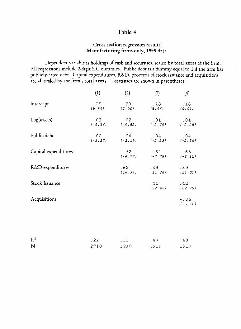
Table 4

Cross section regression results

Manufacturing firms only, 1995 data

Dependent variable is holdings of cash and securities, scaled by total assets of the firm.

All regressions include 2-digit SIC dummies. Public debt is a dummy equal to 1 if the firm has “-”

publicly-rated debt. Capital expenditures, R&D, proceeds of stock issuance and acquisitionsare all scaled by the firm’s total assets. T-statistics are shown in parentheses.

(1) (2) (3) (4)

Intercept

Log(assets)

Public debt

Capital expenditures

R&D expenditures

Stock Issuance

Acquisitions

R2

N

25 23 18 18(;. 89) (;. 00) (~.g6) (;. 01)

-.03 -.02 -.01 -.01(-9.36) (-4.82) (-2. 79) (-.2..28)

-.02 -.04 -.04 -.04(-1.27) (-2.19) (-.2.33) (-2.54)

-.62 -.64 -.68(-6.77) (-7.78) (-8.31)

.62 39 .39(16.34) ~11.-26) (11.07)

41 .42~Z.48) (22 . 79)

-.36(-5.16)

.22

2718

.33 .47

1910 1910

.48

1910

Table 5Cross section regression results

Manufacturing firms only, 1995 dataVariables are the same as in the previous table, except the inclusion of regressors

interacted with a dummy= 1 if the firm’s cash holdings exceed 25 percent of total assets. T-.statistics are shown in parentheses.

Intercept

Intercept *HI

Log(assets)

Log(assets)>:HI

Public debt

Capital expenditures

Capital expenditures*HI

R&D expenditures

R&D expenditures*HI

Stock Issuance

Stock Issuance*HI

Acquisitions

Acquisitions*HI

R2

N

(1)

06i4.40)

57~33 . 84)

-.001(-0.79)

-.04(-9. 74)

-.02(-.? .07)

.76

2718

(2)

04;2.20)

52;24.41)

-.001(-0.47)

-.02(-4.05)

-.03(-.? .50)

11;l. 87)

-1.20(-10.17)

11i2.95)

19;4.15)

(3)

04~2.36)

.42(20. 71)

001iO.48)

-.004(-1.06)

-.02(-.?.42)

10L .79)

-1.27(-11.70)

10;2. 79)

11~2. 64)

05;2.13)

18i6.48)

.79 .82

1910 1910

(4)

.05(2.45)

42~20. 85)

001~O.63)

-.004(-0.86)

-.02(-.?.43)

.09(1. 58)

-1.30(-11.97)

10;2. 81)

10;2.36)

06;.2.23)

19i6.57)

-.08(-1.66)

-.29(-3 00)

.821910

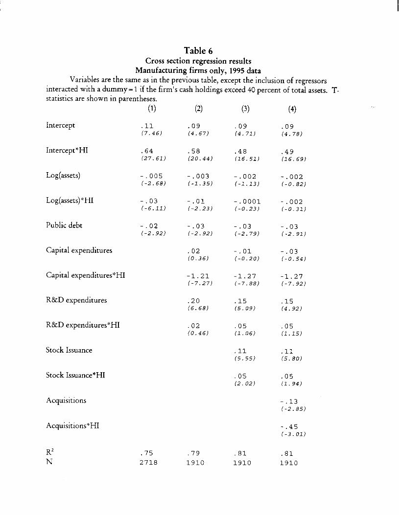
Table 6Cross section regression results

Manufacturing firms only, 1995 dataVariables are the same as in the previous table, except the inclusion of regressors

interacted with a dummy= 1 if the firm’s cash holdings exceed 40 percent of total assets. T-

statistics are shown in parentheses.

Intercept

Intercept *HI

Log(assets)

Log(assets)*HI

Public debt

Capital expenditures

Capital expenditures*HI

R&D expenditures

R&D expenditures*HI

Stock Issuance

Stock Issuance*HI

Acquisitions

Acquisitions*HI

R2N

(1)

11~7.46)

64;27. 61)

-.005(-2.68)

-.03(-6.11)

-.02(-.2.92)

.75

2718

(2)

09~4 . 67)

58;20. 44)

-.003(-1.35)

-.01(-.2’ ..23)

-.03(-.?.9.2)

0210.36)

-1.21(-7.27)

20;6. 68)

02iO.46)

(3)

09;4. 71)

.48(16.51)

-.002(-1.13)

-.0001(-0.23)

-.03(-2. 79)

-.01(-0.20)

-1.27(-7.88)

15;5. 09)

.05(1.06)

11;5.55)

05;2. 02)

.79 .81

1910 1910

(4)

09~4. 78)

49i16. 69)

-.002(-0.82)

-.002(-0.31)

-.03(-2.91)

-.03(-0.54)

-1.27(-7.92)

15;4.92)

05;1.15)

11;5.80)

05;1.94)

-.13(-2.85)

-.45(-3.01)

.81

1910

Chart 1

~~

Tcash ard–Securities to Total AssetsAllnonfinancial firms, by size groups

Sma

Largest firms

Chart 2

I

I Cash to Total-1By size group, firms without public debt I

1

0.8

0.6

0.4

0.2

0

_-i

/

Sma

Largest firms

.

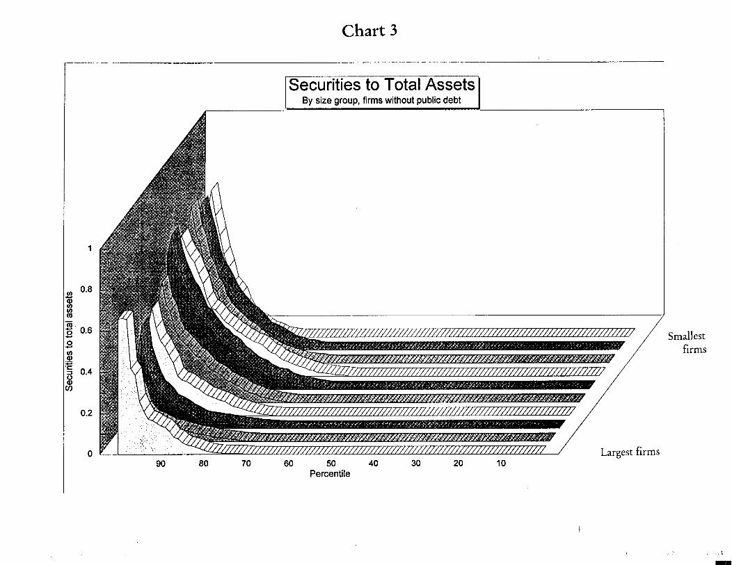
Chart 3

Securities to Total AssetsBy size group, firms without public debt

7’/

Largest

Smallestfirms

firms90 80 70 60 50 40 30 20 10

Percentile

,.. ..$

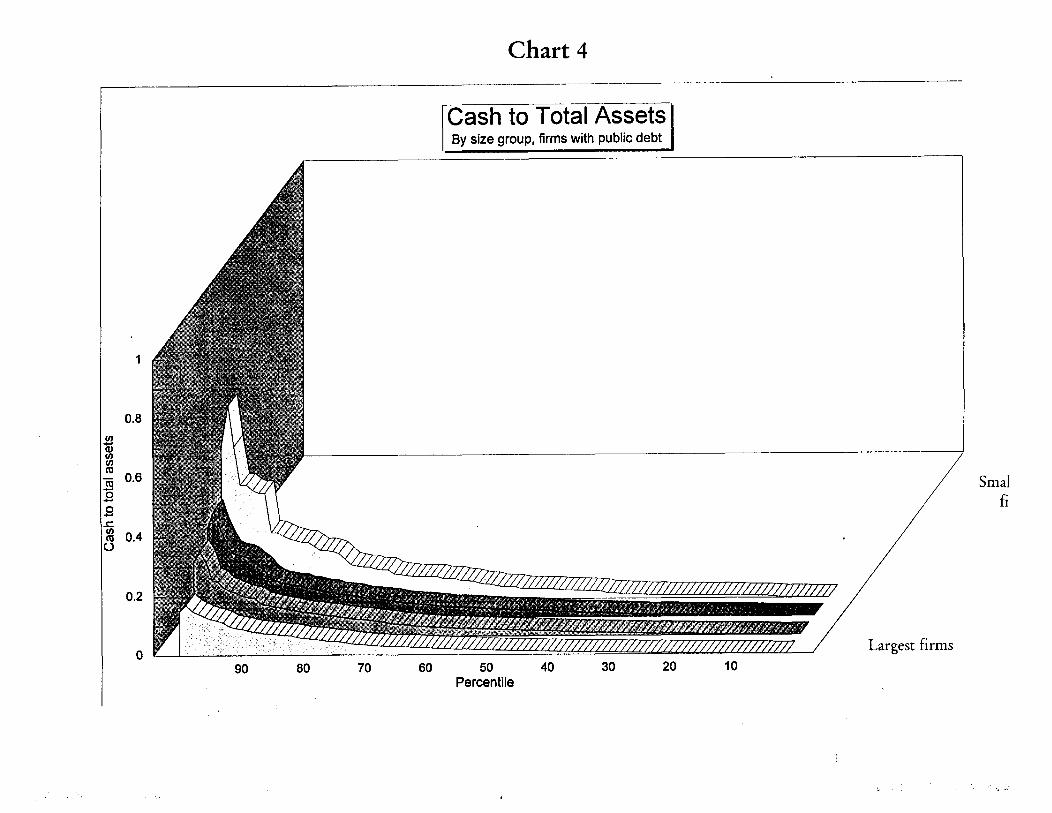
chart 4———. .—

1

0.8

0.6

0.4

0.2

0

ICash to Total A-]By size group, firms with public debt

90 80 70 60 50 40 30 20 10

Percentile

Largest firms

Smallest

firms

.,,.,,.,!. . .. A(

m

Chart 5

. .

—— .. .. .

~ecurities to Total-1By size group, firms with public debt I

1

0.8

0.6

0.4

0.2

090 80 70 60 50 40 30 20 10

Percentile

/

fi:

/

ms

Smallestfirms

-