who supports portable assessment caps: the role of lock-in, mobility and tax share

Regional Science and Urban Economics 41 (2011) 173–186

Contents lists available at ScienceDirect

Regional Science and Urban Economics

j ourna l homepage: www.e lsev ie r.com/ locate / regec

Who supports portable assessment caps: The role of lock-in, mobility and tax share

Ron Cheung a,⁎, Chris Cunningham b

a Department of Economics, Oberlin College, 233 Rice Hall, 10 N. Professor St., Oberlin, OH 44074, USAb Federal Reserve Bank of Atlanta, 1000 Peachtree Street, Atlanta, GA 30309, USA

⁎ Corresponding author. Tel.: +1 440 775 8971; fax:E-mail addresses: [email protected] (R. Cheung)

(C. Cunningham).1 Nagy (1997) does not find an effect on mobility.

0166-0462/$ – see front matter © 2011 Elsevier B.V. Aldoi:10.1016/j.regsciurbeco.2011.01.001

a b s t r a c t
a r t i c l e i n f o
Article history:Received 1 September 2010Received in revised form 29 December 2010Accepted 5 January 2011Available online 15 January 2011

JEL classification:H71R23

Keywords:Property taxVotingAssessment capLock-inMobilityLocal public financeLocal political economy

Popular support for property assessment caps has been explained as attempts to protect long-time homeowners and to constrain local public expenditures. However, in the absence of a binding cap on millage rates,an assessment limit simply lowers the tax share of low-mobility homeowners at the expense of high-mobilityhomeowners. A recent amendment in Florida made existing exemptions portable, lowering the tax share ofhigh mobility households and raising the tax share of low mobility households. Examining vote share byprecinct, we find that more mobile households support portability but that precincts with larger exemptionsdo not. We also find evidence that voters understood how the amendment impacts their tax share. Support forportability is higher when a city has many out-of-state and thus “exemption-less” immigrants and support islower when mobility in the rest of the tax jurisdiction is high. These findings suggest that voters alterassessment rules to minimize their own tax share.

+1 440 775 6978., [email protected]

2 When combinedreduce local revenusupport these limitaefficiency rather thaHowever, these exp2001;Hoyt et al., 200to be inversely correlpuzzle is why votersutilized by local govePape (2008) suggesinterests and thus ssuggests it is residen

3 Ferreira (2007)permitted counties tchoice whether to alassessment cap is tr

l rights reserved.

© 2011 Elsevier B.V. All rights reserved.

with a cap on millage rates, an assessment cap can significantlyes and expenditures (Downes, 1992; Figlio, 1997). Voters maytions because they believe they will improve local governmentn reduce public services (Citrin, 1979; Ladd and Wilson, 1982).

1. Introduction

Since California voters' approval of Proposition 13 in 1978, fifteenstates have limited the growth in property assessments (Hoyt et al.,2009). The tax protection afforded by such caps may induce house-holds to over-stay in their current home (Bogart, 1990; Stohs et al.,2001; Wasi and White, 2005; Ferreira, 2007).1 If housing matchquality diminishes over time, then this “lock-in” effect fromassessment caps will generate an aggregate welfare loss (O'Sullivanet al., 1995, 1999) and could induce additional construction at theurban fringe (Wassmer, 2008). The leading explanations for popularsupport for property assessment caps are that they are intended toconstrain local public expenditures or to protect long-time home

owners.2 However, in Florida, where an assessment cap has been inplace since 1995, few cities have tax rates near the cap, discountingthe first hypothesis. Then in 2008, voters passed a novel amendmentto make the existing exemption portable, calling the secondhypothesis into question and providing the subject for our empiricalanalysis.3

ectations are often not realized (Doyle, 1994; Figlio and Rueben,9). In addition, voters' estimation of government efficiency appearsatedwith their personal tax liabilities (Cutler et al., 1999). A relateduse state referenda to constrain a revenue source that is primarilyrnment. The common explanation is agency failure: Anderson andt that current voters do not trust future voters to guard theireek institutional barriers to future taxes, while Vigdor (2004)ts of other cities in the same state that voters guard against.examines an amendment to California's Proposition 13 thato port the exemptions of residents 55 and over. Counties had alow the portability or not. Oregon has a system in place where theansferrable to new owner, but it is not portable.

http://dx.doi.org/10.1016/j.regsciurbeco.2011.01.001

mailto:[email protected]

mailto:[email protected]

http://dx.doi.org/10.1016/j.regsciurbeco.2011.01.001

http://www.sciencedirect.com/science/journal/01660462

6 Note that for long time homesteaders, assessed value will continue to rise even ascurrent property value declines. In a time of declining house prices, the assessed valuewill gradually catch up with current market value. This is mandated by the provisionsof SOH.

7 Florida is a relative latecomer among the states in passing a property taxlimitation. Shadbegian (1998) points out that by 1992, half the states had passed somelimitation measure. However, some of the states passed measures that did not limitannual assessment increases, which made it possible for local jurisdictions to overridethe limitation by inflating assessed values, while others directly capped revenue andforced jurisdictions to reset the millage rate.

8 Popular press cited large families that had outgrown their starter homes andretired empty-nesters who wanted to downsize, but neither group could afford to paythe additional property taxes that would come with a new house.

174 R. Cheung, C. Cunningham / Regional Science and Urban Economics 41 (2011) 173–186

By treating newly purchased homes in the same way as currentlyowned homes, the amendment ameliorates the lock-in effect but atthe expense of administrative complexity, greater horizontal inequitybetween recent and longtime homeowners and a faster erosion of theproperty tax base. While the original assessment cap passed withpopular support, there was even greater support for the mobility-enhancing amendment. The portability provision is unusual because itimpacts not only a household's current and future property taxliability and thus the finances of its current city, but also the assessedvalue of any city the household may move to in the future. Formerly,cities were able to rely on a certain amount of turnover in the marketto reset the tax base back to market prices; now the base will only berestored when a first-time or out-of-state homebuyer makes apurchase. In addition, in-state migrants from other parts of Floridacan erode the local tax base faster if they port large exemptions intodistricts that have not experienced much appreciation. Thus, after theportability amendment, local governments must reduce their expen-ditures, raise other taxes or fees, tax non-protected property, or raisethe millage rate, which was almost never constrained.4 Rationalvoters thus had to balance their potential tax savings after a moveagainst potentially higher immediate taxes or fewer public goods.

To explain support for the portability amendment, we combinestatewide assessor property records with precinct level election dataand 2000 census block group data. We predict the share of yes votesbasedon themobility rate and theexisting tax savings (the “taxwedge”)from the existing assessment cap, controlling for average demographiccharacteristics, mean income and partisanship. Despite amendmentsupporters' claims that it would result in a tax reduction for owner-occupied property, we do not find higher support for the measure inprecincts with a greater share of homesteaded property. Nor wassupport explained by the average size of a homeowner's current taxexemption, even though an existing exemption is a necessary conditionfor lock-in to occur. Instead, we find that precincts with more mobilehouseholds, and ones more mobile relative to other households in thesame tax jurisdiction, were more likely to support portability. Inaddition, when examining inter-tax district migration, supportincreases when a jurisdiction has high rates of in-migration fromother states but decreases with high rates of in-state migrants. Thesefindings are consistentwith voters understanding themechanics of howportability affects their property tax shares. We believe that voters'behavior was motivated less by immediate tax savings and more by anattempt to shift the burden of financing government back to low-mobility households and especially to new homeowners in Florida.

Section 2 details the original Save Our Homes exemption and theproposed portability amendment. Section 3 lays out the theoreticalframework. In Section 4, we describe the econometric specificationand the dataset, and we explain how we construct our independentvariables of interest. Section 5 presents the initial results for the effectof mobility and wedge on support for portability. Section 6 looks formore sophisticated voter behavior by introducing a measure ofrelative mobility within the city and decomposing types of in-migration. There is a brief conclusion.

2. Institutional detail

Since 1980, Florida law has exempted the first $25,000 of marketvalue from assessment on a homeowner's primary residence or“homestead.”5 In 1995, 54% of Florida voters approved changing the

4 Florida law limits the municipality property tax rate to 10 mills. In 2008,calculations by the authors show that of 388 municipalities, the median municipalmillage rate is 4.1 mills. The municipality at the 95th percentile has a millage rate of7.7 mills, comfortably below the cap.

5 In addition to the standard $25,000 homestead exemption, there is also a $500exemption for a disabled homeowner, a $500 exemption for a widow or widower anda $5000 exemption for a disabled veteran. Beginning in 1997, local jurisdictions cangrant exemptions to senior citizens (Section 193.155(1), F.S.).

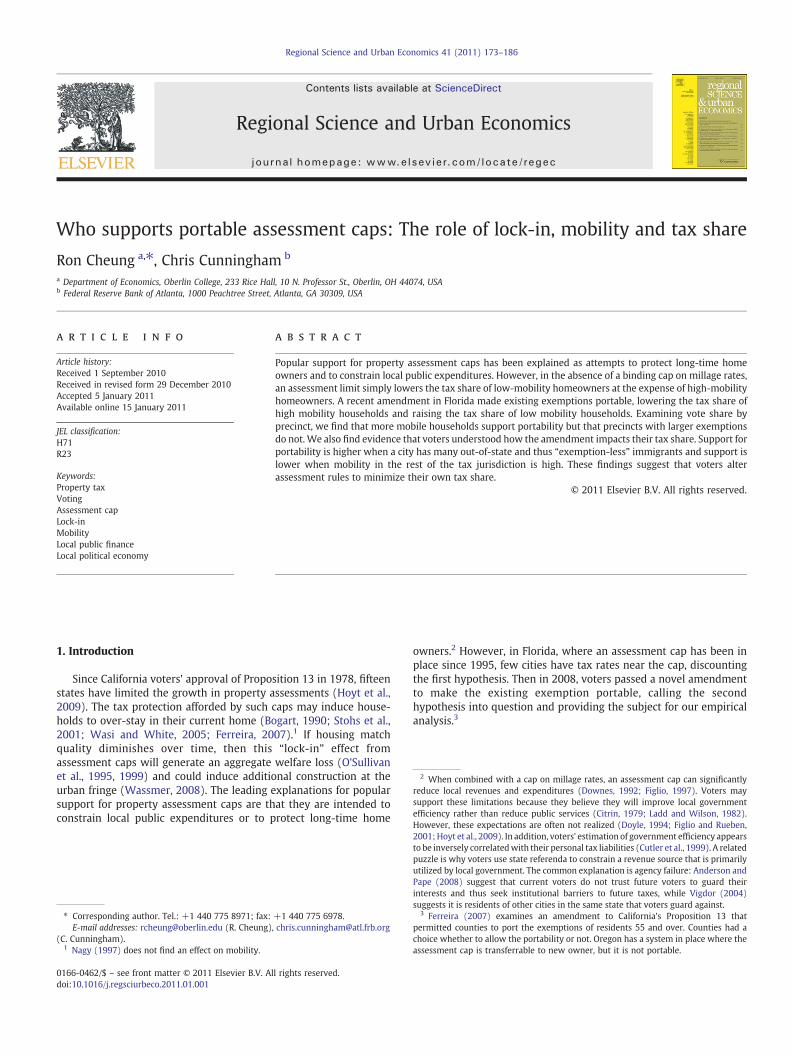
state's constitution with the “Save Our Homes” (SOH) amendmentwhich capped yearly increases in assessed value to the lesser of threepercent or the rate of inflation (based on the CPI for urbanconsumers). Fig. 1 shows the growing “wedge” between market andassessed values that resulted. The light bars represent the annualcapped increase in property values for every year since SOH'sinception. In most years, the inflation rate (based on the previousyear) represents the binding cap. For comparison, the dark bars showthe annualized appreciation in the FHFA house price index. After a fewinitial years of low appreciation, many parts of Florida enjoyedextraordinary house price appreciation. For instance, house pricesincreased by 130 and 108% in Miami and Tampa, respectively,between 1995 and April 2008 (Case–Shiller repeat sales index).Fig. 1b demonstrates how the assessment cap results in a long-heldproperty having nearly half of its value untaxed. The dashed linerepresents the market value of a house that was bought on December31, 1994, and that enjoys the statewide appreciation rate. The solidline represents the assessed value of this house as long as it is notbought or sold. Thanks to Save Our Homes, by 2008, the wedge(vertical distance between the two lines) represents 47% of themarket value of the house and is exempt from property tax.6

The motivation for altering SOH, like that for Proposition 13 inCalifornia and similar measures to cap the growth in assessments, wasthat the assessed value of a property reset to themarket price upon sale,significantly increasing the property tax bill for the new owners.7 Thefear of losing the benefit of a large untaxed wedge was thought to lockfamilies into their existing homes.8 This fear of constraints on mobility,combined with the popular perception that property taxes were toohigh, created support to reform SOH.9 On January 29, 2008, 64% ofFloridians voted to approve “Amendment 1.” The law went into effectfor 2008 property taxes and had four provisions: (1) the homesteadexemption doubled to $50,000 for non-school taxes; (2) the home-owner's tax wedge was made “portable” to other homes within thestate; (3) a $25,000 tangible personal property exemptionwasprovidedto businesses; and (4) assessment growth on non-homesteadedproperty, including rental properties, second homes and commercialproperties, was capped at 10% per year (excluding school taxes). The$25,000 increase in the exemption adds some modest progressivity tothe property tax but is small relative to the average value of houses inthe state. The business exemption on personal property was thought tobequitemodest, and the10%caponnon-homesteadassessment growthdoes not appear to lower future non-homestead taxes.10 In summary,most of the benefits of Amendment 1 were expected to be conferred toowners of homestead property. The portability provision generatesroughly half of these savings and is at the center of our analysis.11 Thus,

9 Charlie Crist, who was elected governor of Florida in 2006, campaigned on aplatform of property tax reform. Prior to the passage of the amendment, the governorand the legislature enacted a rollback of 2007 property taxes to 2006 levels, reducingtax revenues by $15 billion.10 In 2006, the statewide average millage rate (including municipal and countytaxes) was 18.47 or less than 2% of just value, Florida's Property Tax Study InterimReport, Legislative Office of Economic and Demographic Research February 15, 2007.11 A pre-reform analysis conducted by Florida TaxWatch projected that over 80% oftax relief would go to homestead property. Briefings, Florida TaxWatch, January 2008.

-10%

-5%

0%

5%

10%

15%

20%

25%

30%

1995 1996 1997 1998 1999 2000 2001 2002 2003 2004 2005 2006 2007 2008

SOH Assessed Value Increase OFHEO House Price Index Increase

$-

$50,000

$100,000

$150,000

$200,000

$250,000

$300,000

$350,000

1995 1996 1997 1998 1999 2000 2001 2002 2003 2004 2005 2006 2007 2008

SOH Assessed Value Market Value

a

b

Fig. 1. a. Comparison of yearly increase in assessed value allowed by save our homes and yearly increase in FHFA state house price index. b. Comparison of assessed value andmarketvalue of a hypothetical home*.* This graph is based upon the following assumptions: (1) A house is bought for $100,000 on December 31, 1994; (2) It is homesteaded and is notbought or sold thereafter; and (3) Its value appreciates at the same rate as the statewide FHFA house price index.

175R. Cheung, C. Cunningham / Regional Science and Urban Economics 41 (2011) 173–186

we will refer to Amendment 1 as “the portability amendment”throughout the text.

The universal statewide portability of the assessment wedge isunique among the states. If one moves into a home of greater value,the total value of the wedge from the past home is transferred to thenew home up to a maximum portable cap of $500,000. An examplemay be useful. If a homeowner purchased a home in 1994 for$100,000 that by 2008 has a just value of $270,000 and an assessedvalue of $140,000, then thewedge betweenmarket price and assessedprice is $130,000. If the homeowner moves up to a home with a justvalue of $300,000, then without portability the assessed value of thenew house is $300,000.12 With portability, the assessed value isreduced to $170,000 ($300,000–$130,000).13 This assessed valuewould then rise subject to the yearly cap. A homeowner who insteadchooses to buy a cheaper house would get to keep the tax wedgepercentage of the former house. For example, if the new home

12 Local taxes would then be levied on the assessed value less the original exemptionof $25,000 available to all homesteaders. For clarity, we can ignore this in the example.13 Note that these values were not chosen randomly but instead conform to the stateaverage appreciation rate and caps from Fig. 1a.

were worth $230,000, the new assessed value would be $110,740(230,000×(130,000/270,000)).

Voters confronted a difficult calculation of projected benefits andcosts in deciding whether or not to support the referendum.14 In thenext section, we review how changes in the method of assessmentwould change the taxes of different types of voters and thus theirsupport for the portability amendment.

3. The property tax under different assessment regimes

An individual voter's tax bill, T, before an assessment limit can beexpressed as:

T = τ V−25Kð Þ ð1Þ

where τ is the jurisdiction's property tax (millage) rate, V is theassessed value of the house and all homes receive a standard $25,000

14 Many county appraisers have found it necessary to post instructions on theirwebsites explaining to homeowners how to calculate their portable benefits. Anexample is found on the Leon County Property Appraiser's website: http://www.leonpa.org/documents/portability.pdf.

http://www.leonpa.org/documents/portability.pdf

http://www.leonpa.org/documents/portability.pdf

Fig. 2. Lock-in effect of assessment cap and portability on housing consumption. Note: To highlight the impact of the wedge between market and assessed values in this figure weshow the current budget when inflation is greater than 3% (the nominal cap in assessment growth) which generates a discontinuity for consumption of the current home. A similargraph with real house price appreciation above the inflation cap would pivot the budget line in similarly stranding the household in the current home.

16 An alternative diagram with real house price inflation would be similar but wouldshift the budget set in for any housing consumption other than the current one.17 There is still a kink in the budget set from the differential treatment of a “trade-up”or a “trade-down.”18 And, if bequests are to be considered, heirs are satisfied as well.19 They must also make some judgment as to the trajectory of future house prices. If


exemption.15Without Save Our Homes, V is also themarket value.Wecall this assessment regime the “initial regime.” The introduction ofthe original SOH legislation in 1995 capped the growth in assessedvalue at the lesser of inflation or 3%. Thus, the tax T was the millagerate multiplied by the difference between the lesser of the cappedvalue or the market price and the basic exemption:

T = τ min V�;V

� �−25K

� �: ð2Þ

The difference between a home's market value and assessed valueis the assessment wedge, W, which we define as max(V−V

–, 0). Prior

to the portability amendment, moving to a new house resets W tozero. We call this assessment regime the “SOH regime.”

The amendment doubles the initial homestead exemption andintroduces wedge portability. If purchasing a home of greater value,the wedge is the nominal exemption on the previous home, and, iftrading down, the wedge is capped at the ratio of the previousexemption to market value. Introducing subscripts, the annualproperty tax paid on the first home purchased after the portabilityamendment, T1, depends on the accumulated wedge on the previoushome, W0.

T1 =τ1 V1−W0ð Þ−50KÞ if V1 ≥ V0

τ1 V1 1−W0

V0

� �� −50KÞ if V1 b V0

8><>:

9>=>; ð3Þ

We refer to this last assessment regime as the “portability regime.”Under all three regimes, we can then express the consumption of allother goods, x, as a function of current income less the property tax:

x = y−T: ð4Þ

The lock-in effect created by the original Save Our Homes can beillustrated by Fig. 2. Assume that the average inflation rate exceedsthree percent throughout. A household obtains utility from housing

15 Here and throughout the paper, the “jurisdiction” refers to the city if a householdlives in an incorporated area and to the county if the household lives in anunincorporated area.

and from non-housing consumption, which are represented on thevertical and horizontal axes respectively. The $25,000 (and later,$50,000) flat homestead exemptions are suppressed for clarity. Thefigure shows the budget constraints corresponding to the three taxregimes. Initially, in the absence of a property tax exemption, thebudget set is ab, and the optimal consumption level is h0. The SOHassessment cap generates a discontinuous budget set, (ab⋃c), wherethe owner can consume above the budget line, at point c, byremaining in the current house.16 This differential treatment ofcurrent and future homes can generate a lock-in effect that may lowersocial welfare (O'Sullivan et al., 1999). Passage of the portabilityamendment shifts the budget set out to acd, as the accumulatedwedge from a previous home can be used to increase non-housingconsumption reducing much of the lock-in effect.17 Since the shift ofthe budget set is clearly related to the size of the homeowner'saccumulated wedge, our first hypothesis is as follows:

Hypothesis 1. Support for the portability amendment increases withwedge size.

However, an existing assessment wedge is a necessary, but notsufficient condition for households to experience a lock-in effect. Ifhomeowners are happy with their current residence, then theportability feature benefits them not at all.18 We adopt the O'Sullivanet al.'s (1995) framework, where housing mobility is driven bydecaying housing match quality and households move when thecurrent flow of housing services provides insufficient utility subjectto the fixed cost of moving.19 SOH can be thought of as simply a taxon the number of moves a household makes over their lifetime, aseach move resets one's assessment to the market price and raise theirlifetime property tax.

house prices continue to fall as they had in the year before the portability amendment,then the value of the wedge to be ported will decline over time. On the other hand, iflong-run house prices return to their previous trend of increasing faster than inflation,then a voter would need to consider the value of accumulated wedges in future homes.

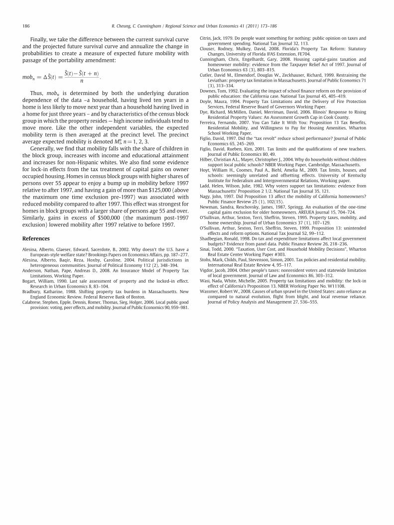
Fig. 3. Lifetimemobility and after-tax consumption under different assessment regimes. Note: B2 and B3 are the life time budget sets under the conventional assessment cap, SOH andwhen accumulated wedges are portable. B2′ and B3′ are the same budget sets when the millage rate is increased to hold revenue constant across regimes. It is the fact that rates mustrise (or expenditures fall) that produces a tension between high and low mobility households affecting support for the portability amendment.


We illustrate this in Fig. 3 by graphing the permanent budget setwhen households consume only mobility and after-tax consumption.Each move incurs transactions costs, such as the commissions on thesale of a previous home. Were mobility costless, this figure would be aflat line ending at life time income. The initial budget set is denotedmr. Passage of SOH steepens the budget set, to pr, as lower mobilityreduces the life-time tax burden and allows greater non-mobilityconsumption. Passage of the portability amendment shifts the budgetset out to ps, which is parallel to the pre-SOH line. Thus householdswith a low taste for mobility (a low rate of decay in match quality)benefit more under a SOH regime and households with a high taste formobility benefit more from portability. This gives rise to a mobility-related hypothesis.

Hypothesis 2. Support for the portability amendment increases withhousehold mobility.

So far we have failed to offer any reason from a homeowner'sbudget standpoint to oppose Save Our Homes or the portabilityamendment. However, over time, Save Our Homes erodes ajurisdiction's base of assessed value. Portability further erodes thebase because portability allows new movers to the jurisdiction toimmediately reduce their assessed value below the market value ofthe new home. Jurisdictions that formerly relied on householdmobility to reset assessed values to market values will find their taxbase shrink (or fail to grow), forcing local governments to: increasethe millage rate; increase some other taxes or fees; reduce publicservices; or pursue some combination of the above.

Much of the literature on assessment caps dwells on voters desireto limit expenditures and many opponents claimed it would harmpublic services.20 However, in Florida some form of rate increaseseems an equally plausible response. First, as the nominal cap on themillage rate is not binding, local governments can respond by simplyincreasing the tax rate. Florida voters may, in fact, anticipate such apolicy response as county assessors are compelled by the state's Truth

20 Two examples of anti-amendment headlines appeared in the Miami Herald in themonths leading up to the vote: “New Florida Residents Target Save Our Homes”(January 27, 2008) and “Tax Reform to Mean More Budget Cuts.” (November 29,2007).

in Millage Act (passed in 1980) to mail each property owner the “roll-back” millage rate on the homeowner's tax bill — the rate that wouldleave revenue unchanged net of new construction.21 We examine thetax share implications when revenue, Rj is held constant byendogenizing the tax rate, τi. In Fig. 3, a higher millage rate wouldpull the entire budget frontier in. We represent this effect by thebudget constraints nq and mr for the SOH and portability regimes,respectively. Whether one is better off under SOH or portabilitydepends on one's lifetime mobility. Households with low mobilityattain a higher indifference curve under budget constraint nq thanunder mr, and so they oppose the portability amendment; theopposite is true for high mobility households.

To see this more clearly, note that in the case when revenue is heldconstant, a household's tax liability is determined by the property'sshare of the total assessed value in the jurisdiction (the tax base), Bj:

T =VBjRj: ð5Þ

The greater the Bj, the smaller are the individual's tax share andtax. However, Bj, is just the sum of the market values of all taxableparcels in the jurisdiction, less total wedges:

Ti =Vi−Wi

∑Vn−∑WnRj: ð6Þ

The portability amendment, therefore, alters how ∑Wn erodesthe tax base.While the amendment increases a household's wedge forthe next home, lowering tax share then, it can raise the tax burden inthe current home, as other movers port their wedges and shrink thedenominator in Eq. (6). More precisely, note that the ∑Wn can bedisaggregated into the sum of wedges of non-migrants (stayers), less

21 When property prices were rising, this rate would tend to fall; however, given therecent correction in house prices, the roll-back rate in many cities exceeds the actualrate. In addition to putting the portability amendment on the ballot, the 2007legislature forced local governments to rescind recent increases in property taxrevenue (lowering future non-school tax revenue between 3 and 9% for mostmunicipalities) and made the existing roll-back rate the statutory rate (Clouser andMulkey, 2008).

image of Fig.�3

23 Before taking the log, we add a 0.01 so as not to exclude the several precincts thatvoted 0% in favor of the amendment. Removing these precincts from the sample didnot change the results qualitatively.24 We do not expect that the three counties dropped to distort our results greatly.They are small: Union, Sumter and Santa Rosa counties have 2007 estimatedpopulations of 14,991, 72,246 and 147,044, respectively (US Census Bureau).25 Assessors use standard appraisal techniques (comparables and replacement costvaluation) to determine the just value. In addition, there is a state requirement that ahome be physically inspected at least once every five years.26 We exclude multifamily residences (but not townhomes) for three reasons:(1) there appears to be a lack of uniformity in how assessors report these properties to


the wedges that sellers take with them, plus the wedges buyers portinto their new homes:

Ti =Vi−Wi

∑Vn− ∑Wstayersn −∑Wseller

n + ∑Wbuyern

� �Rj: ð7Þ

Under Save Our Homes but before portability, the reset provisionset Wn

buyer to zero. However, after portability, Wnbuyer will be non-zero

if the purchaser previously sold a home with an exemption in Florida.Thus, the portability amendment can raise or lower homeowners'lifetime tax burden depending not just on their own mobility, but onthe mobility of other households in the city. Holding a voter's ownmobility constant, higher mobility by other households in thejurisdiction raises the lifetime tax burden and should lower supportfor portability:

Hypothesis 3. Support for the portability amendment falls as the rateof mobility in the rest of the tax jurisdiction increases.

The ability to port wedges across jurisdictions introduces a finalelementof complexity into the voter's decision. If amigrant possessing alarge wedge in one Florida city moves to another city that hasexperienced less appreciation, it will raise the assessment share of theexisting residents in the destination city, holding others' mobilityconstant. This concernwas voiced at the time of the vote by some northFlorida counties, who feared an influx of south Florida residents portinglargewedges and thus forcingbudget cuts or rate hikes. Voters generallymay have responded to this concern, as electoral support for theportability amendment was much lower in relatively affordable northFlorida than in expensive south Florida. The impact of different types ofmobility can be summarized in the fourth empirical hypotheses:

Hypothesis 4. Support for the portability amendment increases asthe relative size of migrant wedges falls.

The balance of the paper tests these four alternative hypothesesempirically.

4. Data

This study combines precinct-level vote shares for the portabilityamendment with parcel level information on market and assessedproperty value, homestead status and date of purchase. We describethem in detail in this section.

4.1. Election data

The unit of analysis is the election precinct, whose boundaries aredetermined by each of the 67 counties in Florida. The smallest countyin our sample has 8 precincts, while the largest county has 711. Theportability amendment appeared on the ballot in the January 29,2008, presidential primary election. All voters had the opportunity tovote on the amendment, and registered Democrats and Republicansalso got to vote for a presidential candidate.22 We obtained from theFlorida Department of Elections the complete statement of votes atthe precinct level. We supplemented this with GIS data of the 2008election precincts from the Department of Elections for each county. Itwas not possible to obtain election results from Union County andSumter County, so these counties were not included in our analysis.

22 We note that the winner of the Democratic primary could not receive anyconvention delegates because of a party sanction for moving the vote forward.Republican candidates received half their assigned delegates. Also, none of the leadingDemocratic candidates campaigned in Florida. Thus, Democratic turnout may havebeen depressed. We attempt to correct for political differences among precincts insome of our specifications later on.

Our dependent variable denoted yi, is ln((number of yes votesdivided by the total number of votes)×100+0.01).23 There wereother notable races on the ballot, and not all voters cast a vote for oragainst the portability amendment. When the votes were counted,however, it was a clear victory for portability. Out of 67 counties, 53had majorities in favor. There were counties that supported theamendment throughout the state, but support was especially strongin south Florida. Miami-Dade, Palm Beach and Broward counties eachvoted about 70% in favor. Supporting counties ranged widely fromsmall to large. In contrast, counties where a majority of votersopposed the amendment generally were small and rural. Two notableexceptions were Duval County (Jacksonville) and Leon County(Tallahassee), large counties that both voted majority no.

4.2. Property data from county assessor files

To develop a measure of the tax savings that can be expected, weobtain property-level data from the Florida Department of Revenue's2007 tax roll. This is a complete listing of all parcels (residential andcommercial) and is compiled from county assessors. Santa RosaCounty was dropped from the analysis because variable names couldnot be reconciled with the standardized names used in other counties.This leaves 64 counties and 6475 precincts in our sample.24

Key to our analysis is the homeowners' existing Save Our Homes“wedge,” the difference between the home's market value and itsassessed value, both of which are reported for every parcel. Countyassessors are required to update a home's market (or just) valueyearly, not only to account for market appreciation, but also for anyadditional improvements that may have been made on the parcel.25

The wedge,W, is simply the difference between the just value and theassessed value. We then determine the precinct of each parcel andcalculate the median wedge, Wi, value of that precinct for all singlefamily, owner-occupied properties.26 We also determine the share ofproperty in the precinct that is currently claiming a homesteadexemption.

4.3. Homeowner mobility

We expect that a household that would like to move but have alarge wedge would support the portability amendment to escape thelock-in effect. While we do not observe taste for mobility directly, wecan identify neighborhoods that appear to have faster turnover. Weposit that people living in neighborhoods whose previous residentshave exhibited shorter tenureswould also have shorter occupancies—or would, but for the lock-in effect of Save Our Homes. We alsoattempt to model mobility and predict the expected mobility ofcurrent residents. These measures are described below.

The property level data from the assessors contain the years of thelatest and the second most recent sale of each parcel in the state.Dividing 1 by the average number of years between the most recent

the state; (2) a high degree of reporting error can arise from condo conversions; and(3) some counties appear to aggregate across units to create a single parcel levelvariable. We are also concerned about the high degree of sub-leasing and numberinvestment properties within condo buildings. It is not clear to us whether a condoowner, even one currently (and honestly) claiming a homestead exemption on acondo unit would behave more like a homeowner or as a potential landlord whenvoting.


and the second most recent sale yields a measure of “churn” in theprecinct. We also construct an expected mobility measure byestimating a richly specified semi-parametric hazard model of theprevious and current owners' duration in the home and then predictthe share of homeowners likely to move in the next 1–3 years. Aricher discussion of the expected mobility measure is provided inAppendix A.

Finally, we also rely on the U.S. Census, which asks whether aperson occupied the same residence in 1995 as they did in 2000. Fromthis question we obtain the percentage of each census block groupthat moved within the last five years. We average this measure (andall other census derived block group values described later) byprecinct. As a precinct usually includes more than one block group,and block group boundaries are often not coterminous with precinctboundaries, we weight each block group by its share of the totalnumber of housing units within the precinct.27

A concern in our specification is the inherent simultaneitybetween wedge size and mobility: a homeowner with low mobilityis likely to have built up a substantial wedge by not moving. Weensure identification by relying on lagged values in estimating churnand census mobility measures. In estimating the hazard-derivedmobility, we control for the wedge but exclude it whenwe predict thecurrent owner's duration in the home.

4.4. Other covariates

We control for socioeconomic and demographic factors that mayinfluence the likelihood of voting for the portability amendment,specifically block group level characteristics from the 2000 census:percent non-Hispanic white, percent in various age groups, percentcollege-educated, median household income, median income squaredand the percentage of the housing units that is renter-occupied.28 Inthe same way as the census mobility rate is defined, each housingparcel is assigned the characteristics of the block group within whichit is located. Then, the precinct average of this value is calculated,weighting by share of housing units. We also include GIS-determineddistance to the nearest central business district (CBD) and include adummy if the precinct is located in a central city of the MSA.

Voters may also be governed by ideology andmay have turned outin different numbers because of the disparate treatment of Republicanand Democratic contests. The Florida Senate has available 2000presidential election data disaggregated to the block group level. Wetherefore assign to each parcel in our tax roll the percentage of votescast in the previous open presidential election for Al Gore in that blockgroup. We then take a weighted average (as above) to create aprecinct level variable.29

Finally, there are institutional and cultural differences betweenFlorida counties, and so we include a full set of dummy variables forthe 64 counties. County fixed effects are especially important for tworeasons: (1) property appraisal and tax collection are done at thecounty level, and (2) Florida school districts are coterminous with

27 To elaborate, we create a measure of lot density defined as block group populationin 2000 divided by the number of single family lots and then multiply this value by thesingle family parcels retained from our calculation of the wedge and mobility. Thus, ablock group makes a large contribution to the precinct mean mobility if it has a lot ofparcels in common with the precinct and/or it contains a lot of multifamily housing. Ifthere is no multifamily present, then the weight is simply based on the block group'sshare of total parcels in the precinct. We believe this weighting scheme is superior toone based simply on the coverage ratio of precinct area and block group area; aprocedure often employed when a finer unit of analysis (parcel) is unavailable.28 We also tried specifications with additional covariates including poverty rate.These do not substantively affect the results and are not reported here.29 While results of the Gore vs. Bush election are available by election precinct, theyare based on 2000 election precinct boundaries, which are not necessarily the same as2008 precincts. There is some concern as to the extent of vote misreporting, but webelieve that any under vote should be largely uniform within counties and can thus beabsorbed by county fixed effects.

counties, and a large portion of a homeowner's tax bill goes to thecounty to pay for schools. With the fixed effects, we are able to controlfor different assessment methods, practices and county publicamenity levels. We are thus identifying the impact of tax wedge andmobility on votes across precincts and tax jurisdictions within eachcounty. Table 1 provides summary statistics of the key variables in theanalysis.

5. Analysis

To test our hypotheses, we first estimate a reduced-form linearregression of share of yes votes at the election precinct level oncurrent tax wedges, measures of expected mobility and a set ofcontrols.

The formal specification is:

yi = XiΦ + β1 + Wi + θ1Mi + μi ð8Þ

where yi is the log share of yes votes in the precinct, Xi is the vector ofcontrol variables (which include a full set of county fixed effects),Wi isthe median size of the tax wedge, Mi is a measure of average mobilityand an error term, ui. First, to test Hypothesis 1, we test the nullhypothesisH01: β1=0, the size of themedianwedge did not affect theshare voting yes. Our alternative hypothesis is that precincts with alarger median wedge between market and assessed values will votefor the right to port those tax savings to a new home (Ha1: β1N0).Similarly, to test Hypothesis 2, we test the null hypothesis: H0-2:θ1=0, that the average mobility of a household does not affect theprecinct's share voting yes. The alternative is that precincts withhigher mobility will vote for the right to port those tax savings to anew home (Ha-2: θ1N0).

5.1. Simple mobility measures

Estimation results using simple measures of mobility are reportedin Table 2. All specifications in this table include a set of county fixedeffects, and standard errors are robust to heteroskedasticity. We beginby looking at the median wedge, W. In the simplest regression(Column 1) with no other covariates except county fixed effects, W issignificant and positive as expected, suggesting that the portability ofthe wedge is attractive to precincts with high potential tax benefits.However, the magnitude of the parameter on W is small: increasingthe wedge by $70,000 (the equivalent of increasing the wedge by onestandard deviation) raises the yes share vote by 1.4%. For the precinctwith the mean yes share of 63%, this translates to barely onepercentage point increase. However, this is the only specification inwhich W positively and significantly raises the yes share.

Column 2 provides the parameter estimates after the inclusion of arich set of additional control variables. The yes vote share in a precinctfalls with educational attainment. Living in the central city reduces thelikelihood of support. The precinct's share of non-Hispanic whites andmedian income are insignificant. Precincts with a high share of veryyoung and elderly persons have lower levels of support for theportability amendment. This may reflect greater reliance on the localpublic services that would suffer if portability were to impact localbudgets.

After inclusion of the covariates, the estimated coefficient of W isstatistically non-significant. Given that a positive wedge is anecessary, but not sufficient, condition for Hypothesis 1, we find thesmall and non-significant parameter estimates on the wedge variablestriking and suggestive that support for the portability amendmentmay have been driven by other considerations.

Columns 3 and 4 show that mobility plays an important role indetermining support for portability. The churn measure is positiveand significant, so that precincts with shorter ownership spells aremore likely to support the amendment. The magnitude of the churn

Table 1Summary statistics of variables used.

(1) Full samplea (2) Restricted samplea

Mean S.D. Mean S.D.

Share of votes “yes” (percentage points) 63.1 (12.17) 62.3 (12.22)Wedge in $1000s (market price–capped price) 48.773 (70.043) 0.619 (0.676)Measures of mobility

Moved in the last 5 years (census) 0.501 (0.120) 0.505 (0.126)Moved into district from out of state 0.160 (0.052) 0.154 (0.041)Moved into district from out of county 0.089 (0.053) 0.085 (0.051)Churn (1/previous owner's duration) 0.190 (0.603) 0.195 (0.761)Relative churn — churn/churn in other precincts in tax jurisdiction 1.02 (0.300) 1.02 (0.300)1-yr expected mobility 0.071 (0.013) 0.071 (0.012)2-yr expected mobility (annualized) 0.059 (0.011) 0.059 (0.010)3-yr expected mobility (annualized) 0.055 (0.010) 0.055 (0.009)

Educational attainmentSome college 0.286 (0.065) 0.287 (0.065)Bachelor's deg. 0.145 (0.088) 0.145 (0.088)Graduate deg. 0.083 (0.065) 0.0834 (0.067)

Age compositionAge 0–4 0.056 (0.022) 0.058 (0.021)Age 5–14 0.127 (0.047) 0.129 (0.047)Age 15–17 0.037 (0.014) 0.038 (0.015)Age 18–24 0.076 (0.052) 0.079 (0.058)Age 65 and above 0.189 (0.142) 0.180 (0.142)

Other controlsMedian income (log) 44.0 (19.3) 43.9 (18.7)Non-Hispanic white (percent) 69.5 (27.4) 66.3 (28.7)Share receiving homestead exemption 0.558 (0.221) 0.219 (0.219)Share voting for Gore in 2000 general on 0.507 (0.169) 0.524 (0.176)Racial concentration-tax district 0.40 (0.17) 0.44 (0.15)Racial dissimilarity 49.62 (48.64) 51.53 (43.49)Dummy — central city 0.20 (0.38) 0.44 (0.15)Distance — CBD 12.9 (11.8) 11.4 (8.9)

Observations 6371 3968

a The full sample is the set of all precincts in the 64 counties. The restricted sample is the set of the precincts located in jurisdictions that have 25 or more precincts.


suggests that a one standard-deviation increase in churn increases theyes share by 0.44 percentage points at the mean. The census measureof mobility implies a much larger effect.30 Increasing the 5-yearmobility rate by one standard deviation increases the share yes voteby 2.49 percentage points at the mean. These estimates providesupport for Hypothesis 2.

Column 5 includes both the wedge and the churn measures.Despite the likely correlation between wedge and mobility, includingboth variables does not alter either coefficient estimate. Finally, notevery parcel receives the homestead exemption, usually because it is asecond home or a vacation residence. Column 6 includes thepercentage of the precinct receiving the homestead exemption. Thesign for this variable is negative but non-significant, which may seemcounterintuitive given how favorably homestead property is treatedunder portability. However, with the exception of renters (which wecontrol for) non-homestead property owners are unlikely to be voters.If the property owner could not claim the homestead exemption, it'sunlikely they'd be eligible to vote. Thus, owners in low-homesteadareas may support the measure because there is a large pool of non-homestead property to shoulder the tax burden.31 However, anyshifting would necessarily occur at the city or county level, not theprecinct, so we introduce some additional jurisdiction variables andtest for such tax-share shifting considerations in Section 6.

30 Note that while the census mobility definition encompasses renters who move aswell as owners, we control for the level of renters in the precinct separately.31 On the other hand, the marginal buyer in low-homestead areas may be a non-homesteader and a current resident seeking to maintain their property value couldoppose the portability amendment for the same reason childless couples supportschool bonds (Hilber and Mayer, 2004). We argue that most of the advantage ofshifting the burden onto non-homestead properties occurred with the original SaveOur Homes, and so the extra gain of shifting the portability cost is likely to be secondorder small.

5.2. Predicted mobility measures

Table 3 reports the regression results from specifications incorpo-rating the hazard-derived measures of mobility. Again, mobility seemsto play an important role in support for the portability amendment.Whether we include ameasure of expectedmobility 1, 2, or 3 years intothe future (Columns 1, 2 and 3), the estimated parameter is significantand positive.32 The magnitudes are in line with the census mobilitymeasures; increasing the 1-year expectedmobility rate by one standarddeviation increases the yes share by 0.30 percentage points at themean.The impact is about four times greater for two-year mobility. However,the coefficient estimate on wedge size remains non-significant.

Now, if expected future house price appreciation is modest, then anexisting wedge and future mobility is necessary for portability to lowerfuture taxes. In Column 4, we interact wedge size and predicted 1-yearmobility. The (wedge×mobility) interaction is positive and significantat the five percent level. This suggests that mobile households with alarger tax wedge were more likely to support the portabilityamendment. These results lend further support for Hypothesis 2.

Finally, we control for underlying political ideology to guard againstconcerns about the irregular Democratic and Republican primaries.Column 6 of Table 2 includes the percentage of the precinct thatsupported Al Gore in the 2000 presidential election. The estimatedcoefficient is negative and highly statistically significant. To the extent

32 The standard errors may suffer from a generated-regressor problem as theexpected mobility measures were created by predicting the survival in the home ofeach property owner and then averaging this value for each precinct. There is no readyanalytical method for correcting the errors when the first stage is estimated at a lowerlevel of analysis. Experiments with bootstrapping the errors for two randomly drawncounties did not appear to grow our estimated standard errors, however any attemptto employ this strategy for the entire state would be very computationally intensive.Instead we treat Table 3 as a robustness check of the churn and census mobilitymeasures.

33 This measure is defined in Alesina et al. (2004) as 1−∑i

groupið Þ2 where groupi is

the share of the population in the tax district that is non-Hispanic white, non-Hispanic

black and Hispanic, respectively.34 We also consider the possibility that voters do not perceive the overall racialcomposition of their city or town but instead look only at their immediatesurroundings so we create an alternative measure: racial heterogeneity at the censustract level. Again, because these indices are calculated at a geographical level differentfrom the precinct, we weight the indices at our unit of analysis. Qualitative resultsfrom these measures are not significantly different, and so they are not reported here,although they are available from the authors.

Table 2Determinants of vote share — wedge and simple mobility measures. Dependent variable=ln([Yes votes/(Yes+No)]×100+0.01).

(1) (2) (3) (4) (5) (6)

Wedge Additional controls Churn Census 5-year mobility Wedge+churn +Share with homestead exemption

Wedge (just — assessed value) 0.0002** 0.00004 0.00003 −0.0001+

(0.0001) (0.0001) (0.0001) (0.00007)Churn 0.012** 0.012** 0.014**

(0.003) (0.002) (0.003)Census mobility rate 0.316**

(0.076)% with homestead exemption 0.105

(0.072)Some college −0.067 −0.063 −0.129 −0.065 −0.112

(0.111) (0.111) (0.104) (0.112) (0.112)Bachelor's deg. 0.269 0.283 0.182 0.281 0.260

(0.224) (0.230) (0.221) (0.227) (0.219)Graduate deg. −0.470** −0.472** −0.470** −0.479** −0.461**

(0.179) (0.175) (0.171) (0.181) (0.179)Age 0 to 4 −0.782+ −0.781+ −1.400** −0.780+ 0.860+

(0.412) (0.412) (0.447) (0.412) (0.443)Age 5 to 14 −0.271 −0.240 −0.091 −0.244 −0.256

(0.241) (0.245) (0.260) (0.242) (0.237)Age 15 to 17 −0.820 −0.685 0.103 −0.694 −0.895

(0.742) (0.740) (0.805) (0.748) (0.800)Age 18 to 24 −0.095 −0.074 −0.164+ −0.075 −0.082

(0.090) (0.090) (0.089) (0.091) (0.093)Age 65 and above −0.165** −0.122** −0.097* −0.123** −0.145**

(0.043) (0.044) (0.048) (0.044) (0.047)Median income 0.001 0.0004 0.0003 0.0004 0.0001

(0.002) (0.002) (0.002) (0.002) (0.002)Median income2 1.90e−6 2.42e−6 2.68e−6 2.38e−6 4.77e−6

(8.00e−6) (8.29e−6) (8.11e−6) (8.24e−6) (9.27e−6)Non-Hispanic white 0.0006 0.0007 0.0008 0.0007 0.0007

(0.0005) (0.0005) (0.0005) (0.0005) (0.0005)% Renters −0.0002 −0.0002 −0.001+ −0.0002 −3.42e−6

(0.0005) (0.0005) (0.0006) (0.001) (0.0005)Precinct located in central city −0.034** −0.033** −0.025* −0.033** −0.033**

(0.012) (0.012) (0.012) (0.012) (0.012)Distance to CBD −9.28e−7 −0.0001 0.0001 −0.00004 −0.00002

(0.001) (0.001) (0.001) (0.001) (0.001)Constant 3.853** 4.006** 3.984** 3.874** 3.987** 3.961**

(0.032) (0.071) (0.067) (0.079) (0.072) (0.065)Observations 6473 6471 6428 6471 6428 6428R-squared 0.211 0.222 0.221 0.227 0.222 0.223

All specifications include county fixed effects. For scaling purposes, wedge is measured in $1000s. Robust standard errors in parentheses. +Significant at 10% level; *Significant at 5%level; **Significant at 1% level.


that the variable represents a relatively liberal precinct, this resultsuggests that voters on the political left are less likely to supportportability. Still, controlling for ideology does not change our parameterestimates for wedge or mobility.

Alternatively, voters may have expected local governments tomaintain revenues by raising taxes on other types of property.

5.3. Presence of racial and ethnic heterogeneity

We now expand the specification to accommodate alternativeexplanations of voter behavior. Leading up to the amendment,proponents claimed that it would lower taxes, while many opponentsof the measure claimed it would adversely affect the budgets ofmunicipal and county governments. This suggests that both proponentsand opponents may have expected local governments to respond toportability, in part, by cutting expenditures. Examining countygovernment data, Alesina et al. (2002) find evidence that racialheterogeneity may lower expenditures on public goods because votersare less able to identify with likely recipients or because likelybeneficiaries find it harder to form political coalitions across ethniclines. Voters may care more about the tax savings and individualbenefits of portability if they do not support the redistributive effects oflocal public services that benefit racial or ethnic groups other than their

own. We formulate two measures of dissimilarity, both based on therace categories from the Census. The first is a measure of racialheterogeneity that is the probability that two randomly drawnindividuals in a municipality will be of a different race.33 The second isthe coefficient of dissimilarity that measures the degree of segregationacross a municipality for any given level of racial heterogeneity in thepopulation. A larger value suggests that blacks and Latinos are moregeographically concentrated within the jurisdiction.34

The first two columns of Table 4 present the estimates. Controllingfor share non-Hispanic white at the precinct level, Column 1 shows thatmore heterogeneous cities were less likely to support the portabilityamendment which in inconsistent with more heterogeneous

35 Dye et al. (2006), for instance, show that the residential assessment cap in Illinoisresulted in higher tax bills for commercial property owners and residents ineligible forthe cap. See Bradbury (1988) and Calabrese et al. (2006) for similar evidence fromMassachusetts.36 There is of course a potentially off-setting consideration. Current homesteaders arepotential sellers to non-homesteaders. If the marginal buyer of homes in a givenneighborhood is likely to be a snow-bird (non-homestead recipient) the current votermay oppose the portability amendment for fear of jeopardizing their home values.However, this effect is likely to be small and second order.

Table 3Robustness check/alternative measures of mobility/controls for partisanship. Dependent variable=ln([Yes votes/(Yes+No)]×100+0.01).

(1) (2) (3) (4) (5)

Expected mobility Wedge×mobility Political indicator

1-year 2-year 3-year

Wedge −0.0001 −0.0001 −0.00001 −0.0002+ −0.0001(0.0001) (0.0001) (0.00004) (0.0001) (0.0001)

1-yr exp. mobility 0.375** 0.338* 0.343**(0.129) (0.132) (0.131)

2-yr exp. mobility 1.399**(0.530)

3-yr exp. mobility 0.093(0.177)

Wedge×1-yr mobility 0.001* 0.001*(0.0004) (0.0004)

Vote for Gore −0.264**(0.030)

% with homestead exemption 0.036 0.107 −0.054* 0.038 0.018(0.053) (0.081) (0.022) (0.054) (0.055)

Some college −0.078 −0.084 −0.095+ −0.077 0.007(0.100) (0.106) (0.052) (0.100) (0.103)

Bachelor's deg. −0.078 0.367+ 0.133 0.160 0.216(0.100) (0.206) (0.126) (0.138) (0.139)

Graduate deg. −0.553** −0.520** −0.582** −0.558** −0.417*(0.167) (0.177) (0.138) (0.167) (0.165)

Age 0–4 −0.342 −0.697* −0.120 −0.332 −0.285(0.220) (0.347) (0.196) (0.218) (0.215)

Age 5–14 −0.358+ −0.265 −0.567** −0.336 −0.122(0.214) (0.234) (0.114) (0.218) (0.216)

Age 15–17 −1.270+ −1.163 −0.704** −1.237+ −1.035(0.746) (0.785) (0.267) (0.742) (0.752)

Age 18–24 −0.147* −0.167** −0.124* −0.130* −0.074(0.064) (0.063) (0.061) (0.064) (0.062)

Age 65 and above −0.167** −0.166** −0.135** −0.161** −0.072+

(0.037) (0.039) (0.031) (0.036) (0.040)Median income 0.002 −0.001 0.004** 0.002 −0.0003

(0.001) (0.003) (0.001) (0.001) (0.001)Median income2 −3.09e−6 8.20e−6 −0.0001** −4.76e−6 5.25e−6

(5.86e−6) (9.79e−6) (3.47e−6) (5.46e−6) (5.98e−6)Non-Hispanic white 0.001** 0.001** 0.001** 0.001** −0.0001

(0.0002) (0.0003) (0.0002) (0.0002) (0.0002)% Renters −0.0001 −0.0003 −0.0001 −0.0001 −0.0004+

(0.0002) (0.004) (0.0002) (0.0002) (0.0002)Precinct located in −0.020* −0.022* −0.030** −0.021** −0.017*central city (0.008) (0.087) (0.005) (0.008) (0.0007)Distance to CBD 0.001+ 6.18e−6 0.001* 0.001+ 0.001+

(0.001) (0.001) (0.0004) (0.001) (0.001)Constant 3.898** 3.757** 3.969** 3.895** 4.077**

(0.072) (0.113) (0.066) (0.072) (0.076)Observations 6338 6307 6274 6338 6338R-squared 0.382 0.265 0.541 0.382 0.392

All specifications include county fixed effects. For scaling purposes, wedge is measured in $1000s. Robust standard errors in parentheses. +Significant at 10% level; *Significant at 5%level; **Significant at 1% level.


population being more tax averse. However, Column 2 finds thatcontrolling for a given level of racial and ethnic heterogeneity, precinctsinmore segregated townsweremore likely to support portability. This isexpected and suggests that cities that are a priori less receptive topotentially redistributive public services (as indicated by their level ofsegregation) are more likely to favor the tax cutting potential of theportability amendment. We take the combined findings as mixedevidence that voters expected portability to actually lower expendi-tures. In any case, these additional controls donot reduce themagnitudeor significanceof themobilitymeasure ormake the coefficient onwedgesize positive.

5.4. Presence of non-homestead and non-residential property

The portability rule affected only homesteaded residential proper-ties. Thus, homesteaded voters may have been more willing to supportportability if they believed that revenue loss from their declining

assessments would be made up by higher taxes on non-homestead ornon-housing property.35 Thus, one explanation for the non-significantparameter estimates on share homestead in the previous regressions isthat a high homestead rate suggests that there are fewer otherproperties that can shoulder the tax burden.36 In Column 3 of Table 4,we include the share of the jurisdiction's tax base that is currentlyreceiving a homestead exemption. Our prior is that a high jurisdictionhomestead rate should lower support while a high precinct homestead

Table 4Curbing expenditure vs. shifting the tax burden? Dependent variable=ln([Yes votes/(Yes+No)]×100+0.01).

(1) (2) (3) (4)

Tax jurisdiction racialheterogeneity

Tax jurisdiction racialdissimilarity

Share of tax base coveredby homestead exemption

Share of tax base byproperty class

Wedge (just — assessed value) −0.0001 −0.00004 −0.00004 −0.00004(0.0001) (0.0001) (0.0001) (0.0001)

Churn 0.012** 0.011** 0.011** 0.011**(0.002) (0.002) (0.002) (0.002)

% with homestead exemption 0.048 0.051 0.035 0.047(0.076) (0.076) (0.067) (0.069)

Vote for Al Gore in 2000 −0.211* −0.203* −0.206* −0.228**(0.089) (0.090) (0.087) (0.077)

Racial heterogeneity (tax jurisdiction) −0.177* −0.202** −0.180** −0.144**(0.072) (0.073) (0.053) (0.044)

Racial dissimilarity (tax jurisdiction) 0.0001** 0.001** 0.0004**(0.0001) (0.0001) (0.0001)

Share of jurisdictions tax basea covered by• Homestead exemption 0.124 −0.107

(0.130) (0.103)• Residential (inclusive of homesteads) 0.516*

(0.213)• Commercial 0.457

(0.293)• Industrial 0.366

(0.372)Constant 4.233** 4.224** 4.187** 3.930**

(0.106) (0.107) (0.115) (0.209)Observations 6393 6393 6393 6393R-squared 0.276 0.279 0.280 0.289

All specifications include county fixed effects and all demographic controls. For scaling purposes, wedge is measured in $1000s. Robust standard errors, clustered at the jurisdictionlevel, in parentheses. +Significant at 10% level; *Significant at 5% level; **Significant at 1% level.

a Excluded category is agricultural, which is assessed based on current use.


rate increases support because it entails a large number of householdsthat could benefit fromportability.37However, the estimated parameteron jurisdiction homestead rate is positive, though not statisticallydifferent from zero. In Column 4, we include three newmeasures of thetax base of the precinct's jurisdiction: the share of the jurisdictional taxbase that is residential, commercial and industrial.38 The estimate on theshare of homesteaded residential land (−0.107+0.516=0.409) is notsignificantly different from share commercial or industrial. It also is notstatistically different from the share of non-homestead residential land.Thesefindings suggest that voters did not expect their local governmentto offset the portability amendment by raising taxes on non-residentialproperties.39

6. Migration and relative mobility

The reason homestead property owners could be ambivalent aboutthe portability amendment is that while they can port an exemptionat some time in the future, so can other homeowners. The ultimate taxburden hinges on their mobility, but also the mobility of fellowresidents. Citizens living in a city where there are many migrantscoming in from other parts of Florida may expect these migrants toput pressure on local expenditures while not contributing to the taxbase— thus dampening support for tax portability. On the other hand,residents living in townswith high rates of migration from out of state

37 Though not shown, Table 4 includes as a regressor the share renting from the 2000census, so we believe the share non-homestead is capturing ownership of secondhomes, a large component of the housing market in Florida.38 These do not add up to 1 because of additional tax base categories such asinstitutional and agricultural property. Agricultural land under Florida's Greenbelt lawis taxed based on current use and is generally difficult to tax.39 This may be because the shifting of the burden onto non-homesteaded propertieswas mostly done at the SOH adoption stage, rather than at the portability amendmentstage. However this is simply a speculation as we do not attempt to test for it in theanalysis.

can rely on these “wedge-less” buyers to reset the assessed value andslow the erosion of the tax base even after the passage of portability.

We augment our reduced-form linear regression equation withadditional measures derived from Eqs. (6) and (7) in Section 3:

yi = XiΦ + β1 + Wi + θ1Mi + I′jγ + θ2 +Mi

Mj+ ej + μ i: ð9Þ

Where Ij is a vector of types of in-migrants to the tax jurisdiction

andMi

Mj, the ratio of mobility in the precinct over jurisdiction average

mobility.Column 1 of Table 5 provides the baseline result for this analysis.

We return to the 2000 census measure of tax jurisdiction (city-level)mobility and precinct level mobility to be consistent with the census-derived migration variables discussed below. This specification alsoincludes all of the jurisdiction tax-base sharemeasures from Column 4of Table 4. While precincts with high rates of mobility are more likelyto support the portability amendment, controlling for precinct (own)mobility, voters in high-mobility jurisdictions do not appear to bemore likely to support the amendment.

However, in Column 2 of Table 5, we include out-of-state mobilityinto the jurisdiction. Cities with a large share of out-of-state (and thuswedge-less) in-migrants are significantly more likely to supportportability. A one-standard-deviation increase in the share ofresidents from out-of-state increases support for the amendment by2.7 percentage points. Given the large magnitude of this coefficientcompared to the previously estimated coefficients, we believe thisevidence is consistent with the tax shifting hypothesis. At the sametime, the parameter estimate on jurisdiction mobility which nowcaptures the effect of in-state migration is negative and significant.Residents in cities with high rates of in-state migration can expect theassessed value of land to grow more slowly as wedges start to be

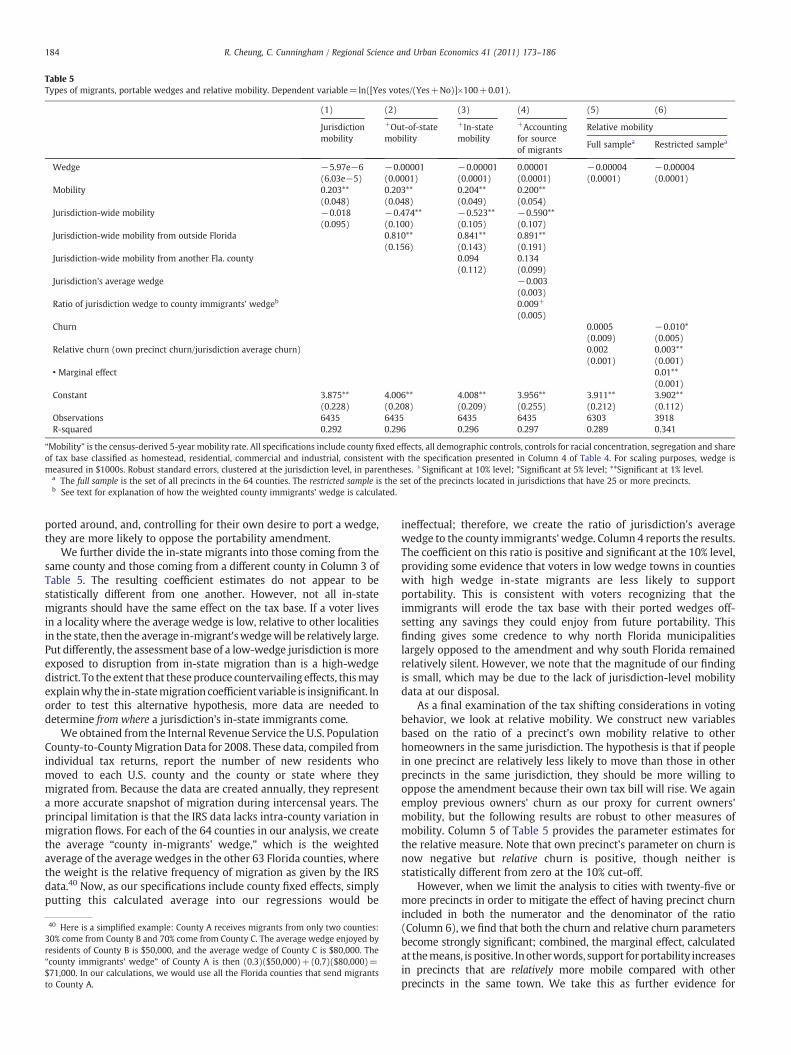
Table 5Types of migrants, portable wedges and relative mobility. Dependent variable=ln([Yes votes/(Yes+No)]×100+0.01).

(1) (2) (3) (4) (5) (6)

Jurisdictionmobility

+Out-of-statemobility

+In-statemobility

+Accountingfor sourceof migrants

Relative mobility

Full samplea Restricted samplea

Wedge −5.97e−6 −0.00001 −0.00001 0.00001 −0.00004 −0.00004(6.03e−5) (0.0001) (0.0001) (0.0001) (0.0001) (0.0001)

Mobility 0.203** 0.203** 0.204** 0.200**(0.048) (0.048) (0.049) (0.054)

Jurisdiction-wide mobility −0.018 −0.474** −0.523** −0.590**(0.095) (0.100) (0.105) (0.107)

Jurisdiction-wide mobility from outside Florida 0.810** 0.841** 0.891**(0.156) (0.143) (0.191)

Jurisdiction-wide mobility from another Fla. county 0.094 0.134(0.112) (0.099)

Jurisdiction's average wedge −0.003(0.003)

Ratio of jurisdiction wedge to county immigrants' wedgeb 0.009+

(0.005)Churn 0.0005 −0.010*

(0.009) (0.005)Relative churn (own precinct churn/jurisdiction average churn) 0.002 0.003**

(0.001) (0.001)• Marginal effect 0.01**

(0.001)Constant 3.875** 4.006** 4.008** 3.956** 3.911** 3.902**

(0.228) (0.208) (0.209) (0.255) (0.212) (0.112)Observations 6435 6435 6435 6435 6303 3918R-squared 0.292 0.296 0.296 0.297 0.289 0.341

“Mobility” is the census-derived 5-year mobility rate. All specifications include county fixed effects, all demographic controls, controls for racial concentration, segregation and shareof tax base classified as homestead, residential, commercial and industrial, consistent with the specification presented in Column 4 of Table 4. For scaling purposes, wedge ismeasured in $1000s. Robust standard errors, clustered at the jurisdiction level, in parentheses. +Significant at 10% level; *Significant at 5% level; **Significant at 1% level.

a The full sample is the set of all precincts in the 64 counties. The restricted sample is the set of the precincts located in jurisdictions that have 25 or more precincts.b See text for explanation of how the weighted county immigrants' wedge is calculated.


ported around, and, controlling for their own desire to port a wedge,they are more likely to oppose the portability amendment.

We further divide the in-state migrants into those coming from thesame county and those coming from a different county in Column 3 ofTable 5. The resulting coefficient estimates do not appear to bestatistically different from one another. However, not all in-statemigrants should have the same effect on the tax base. If a voter livesin a locality where the average wedge is low, relative to other localitiesin the state, then the average in-migrant'swedgewill be relatively large.Put differently, the assessment base of a low-wedge jurisdiction is moreexposed to disruption from in-state migration than is a high-wedgedistrict. To the extent that theseproduce countervailing effects, thismayexplainwhy the in-statemigration coefficient variable is insignificant. Inorder to test this alternative hypothesis, more data are needed todetermine from where a jurisdiction's in-state immigrants come.

We obtained from the Internal Revenue Service the U.S. PopulationCounty-to-CountyMigration Data for 2008. These data, compiled fromindividual tax returns, report the number of new residents whomoved to each U.S. county and the county or state where theymigrated from. Because the data are created annually, they representa more accurate snapshot of migration during intercensal years. Theprincipal limitation is that the IRS data lacks intra-county variation inmigration flows. For each of the 64 counties in our analysis, we createthe average “county in-migrants' wedge,” which is the weightedaverage of the average wedges in the other 63 Florida counties, wherethe weight is the relative frequency of migration as given by the IRSdata.40 Now, as our specifications include county fixed effects, simplyputting this calculated average into our regressions would be

40 Here is a simplified example: County A receives migrants from only two counties:30% come from County B and 70% come from County C. The average wedge enjoyed byresidents of County B is $50,000, and the average wedge of County C is $80,000. The“county immigrants' wedge” of County A is then (0.3)($50,000)+(0.7)($80,000)=$71,000. In our calculations, we would use all the Florida counties that send migrantsto County A.

ineffectual; therefore, we create the ratio of jurisdiction's averagewedge to the county immigrants' wedge. Column 4 reports the results.The coefficient on this ratio is positive and significant at the 10% level,providing some evidence that voters in low wedge towns in countieswith high wedge in-state migrants are less likely to supportportability. This is consistent with voters recognizing that theimmigrants will erode the tax base with their ported wedges off-setting any savings they could enjoy from future portability. Thisfinding gives some credence to why north Florida municipalitieslargely opposed to the amendment and why south Florida remainedrelatively silent. However, we note that the magnitude of our findingis small, which may be due to the lack of jurisdiction-level mobilitydata at our disposal.

As a final examination of the tax shifting considerations in votingbehavior, we look at relative mobility. We construct new variablesbased on the ratio of a precinct's own mobility relative to otherhomeowners in the same jurisdiction. The hypothesis is that if peoplein one precinct are relatively less likely to move than those in otherprecincts in the same jurisdiction, they should be more willing tooppose the amendment because their own tax bill will rise. We againemploy previous owners' churn as our proxy for current owners'mobility, but the following results are robust to other measures ofmobility. Column 5 of Table 5 provides the parameter estimates forthe relative measure. Note that own precinct's parameter on churn isnow negative but relative churn is positive, though neither isstatistically different from zero at the 10% cut-off.

However, when we limit the analysis to cities with twenty-five ormore precincts in order to mitigate the effect of having precinct churnincluded in both the numerator and the denominator of the ratio(Column 6), we find that both the churn and relative churn parametersbecome strongly significant; combined, the marginal effect, calculatedat themeans, is positive. Inotherwords, support forportability increasesin precincts that are relatively more mobile compared with otherprecincts in the same town. We take this as further evidence for

Appendix Table 1Summary of parameter estimates from 66 Cox proportional hazard models of mobility.a

Meanparameterestimate

Positiveb Notsignificantb

Negativeb

Education (share)c

Some college 0.071 24 26 16Bachelors 0.462 28 30 8Graduate degree −0.074 22 34 10

Age distributionShare of pop 5–14 yrs old −0.008 13 30 23Share of pop 15–17 yrs old −1.797 9 27 30Share of pop 18–24 yrs old 0.668 14 32 20Share of pop 65+ yrs old −0.002 12 31 23Income (000s) 0.013 19 33 14Income2 −0.0002 14 33 19Share non-Hispanic 0.0001 17 35 14Distance to CBD −0.001 15 29 22Capital gains (000s)d −0.002 5 24 37

Federal capital gains parametersDummy spell completed pre-97 −1.318 0 3 63Share population over age 55 −0.0002 17 17 32Share population over age55×pre-97

0.0003 35 17 14

Dummy: gainN125K 0.034 29 18 19Dummy: gainN125K×pre-97 −0.642 0 6 60capgainovr125k_pre97age55 0.0001 22 23 21Dummy: gainN500K 0.019 18 27 21Dummy: gainN125K×post-97 −0.201 3 20 43

a Residence spell is defined as the time, in years, between the purchase and sale ofthe home by the previous owner or purchase year and 2008 for the current owner.

b Significance based on a 5-percent cut-off using a two tailed test.c All variables relating to age, education and income are drawn from 2000 census


Hypothesis 4, that voters understand the fundamental shifting in taxburdens that portability would provide. Under the original Save OurHomes provisions, long-stayers could expect the tax burden to slowlyshift to high-mobility households. The portability amendment reversesthat effect and, assuming it leads to an increase in the millage rate orother taxes, causes the tax-share of long duration residents to rise. Thus,the portability amendment acted as away for high-mobility householdsto shift the burden back to the low-mobility ones, and the voting resultsare consistent with this view.

7. Conclusion

While many states have introduced property assessment caps,Florida's Amendment 1 is the first law to allow all owners to port theirexempted value. This policy shift may significantly improve themobility of homeowners and increase the efficient matching ofhomeowners to homes, but at the expense of further horizontalinequity. It is also hard to reconcile the strong support for both theoriginal cap and the portability amendment with a desire to rewardlow or high mobility residence. Also, we find only weak evidence thatvoters were attempting to constrain local expenditures, though thesespecifications are at best an indirect test.

We explore voter support for portability by regressing precinct-level voting data from the portability referendum on the assessmentwedge formed by the difference between the just value and theassessed value of a house and various measures of householdmobility, socioeconomic, geographic and political variables. We findevidence that voters with ex ante high mobility were more likely tosupport the portability amendment but the size of the existing wedgewas not an important determinant. We also found that support washigher in tax districts whose in-migrants were “wedge-less” andsupport was lower when themobility rate in the rest of the tax districtwas higher. However, support was affected by the share of non-homestead properties, perhaps because these properties were alreadytaxed at the revenue maximizing rate. Our results are more consistentwith voters attempting to lower their tax share at the expense offuture Florida home owners.

Acknowledgements

We are grateful to Brad Huff at Florida State University for GISassistance. This paper has benefited from comments from participantsat seminars at the Federal Reserve Board of Governors, Georgia StateUniversity, the University of Melbourne, the University of Adelaideand Florida State University and session participants at the AnnualNational Tax Association and the North American Regional ScienceAssociation meetings. All errors are our own.

Appendix A. Creating a measure of expected mobility

The specification for the hazard of moving function is:

h tð Þ = h0 tð Þ exp X′β� �

where the baseline hazard, h0(t), is estimated non-parametrically andthen shifted proportionally by changes in a vector of covariates X. Weinclude in X Census 2000 controls for the block group that theproperty is located in: income and income squared; share ofpopulation that is non-Hispanic white; educational attainment; andshare of population in the following age groups: 0–4, 5–13, 14–17, 18–24, 25–64, and 64 plus. We also include the property's distance fromthe CBD as a control.41 Building on the work of Sinai (2000), Newman

41 These additional covariates, for the most part, appear in the main voting equationas well, and so they are described in greater detail in the “Other Covariates” section ofthe paper.

and Reschovsky (1987) and Cunningham and Engelhardt (2008), wealso include the following variables to account for lock-in effectsgenerated by the federal treatment on capital gains in owner occupiedhousing: occupancy spell completed before 1997; capital gain inexcess of $125,000; (occupancy spell completed before 1997×capitalgain in excess of 125,000); occupancy spell completed after 1997; and(occupancy spell completed after 1997×capital gain in excess of$500,000). We run each model separately by county yielding 64separate regression estimates. Some summary statistics of theparameter estimates for the county regressions are presented inAppendix Table 1. The full set of coefficient estimates is available fromthe authors upon request.

Using the estimated hazard functions and the coefficient estimateson the covariates, we calculate for each house the survival probabilitythat the current owner will remain in the house (in other words, weignore the previous owners' tenure) and set capital gains to zero topredict survival in the absence of a property tax lock-in effect. Thepredicted survival curve is thus:

S tð Þ = S0 tð Þ exp X′ β� �

where the non-parametrically fitted baseline survival curve, S tð Þ, isshifted proportionally by the exponeniated independent variablemultiplied by the parameter estimates X′ β. Next we estimate theprobability of the current owner remaining in the home n years intothe future. We do this by moving n years (we do this for n=1, 2 or3 years) down the survival curve and then shifting it by the current setof covariates and parameter estimates (excluding capital gains):

S t + nð Þ = S0 t + nð Þ exp X′β� �

:

block group summary statistics.d Capital gain is either the realized gain: sales price less purchase price or for right

censored spells the difference between purchase price and assessor determined “justvalue.”


Finally, we take the difference between the current survival curveand the projected future survival curve and annualize the change inprobabilities to create a measure of expected future mobility withpassage of the portability amendment:

mobn = Δ S tð Þ = S tð Þ− S t + nð Þn

:

Thus, mobn is determined by both the underlying durationdependence of the data –a household, having lived ten years in ahome is less likely to move next year than a household having lived ina home for just three years – and by characteristics of the census blockgroup inwhich the property resides— high income individuals tend tomove more. Like the other independent variables, the expectedmobility term is then averaged at the precinct level. The precinctaverage expected mobility is denoted Mn

i, n=1, 2, 3.Generally, we find that mobility falls with the share of children in

the block group, increases with income and educational attainmentand increases for non-Hispanic whites. We also find some evidencefor lock-in effects from the tax treatment of capital gains on owneroccupied housing. Homes in census block groupswith higher shares ofpersons over 55 appear to enjoy a bump up in mobility before 1997relative to after 1997, and having a gain of more than $125,000 (abovethe maximum one time exclusion pre-1997) was associated withreducedmobility compared to after 1997. This effect was strongest forhomes in block groups with a larger share of persons age 55 and over.Similarly, gains in excess of $500,000 (the maximum post-1997exclusion) lowered mobility after 1997 relative to before 1997.

References

Alesina, Alberto, Glaeser, Edward, Sacerdote, B., 2002. Why doesn't the U.S. have aEuropean-style welfare state? Brookings Papers on Economics Affairs, pp. 187–277.

Alesina, Alberto, Baqir, Reza, Hoxby, Caroline, 2004. Political jurisdictions inheterogeneous communities. Journal of Political Economy 112 (2), 348–394.

Anderson, Nathan, Pape, Andreas D., 2008. An Insurance Model of Property TaxLimitations, Working Paper.

Bogart, William, 1990. Last sale assessment of property and the locked-in effect.Research in Urban Economics 8, 83–104.

Bradbury, Katharine, 1988. Shifting property tax burdens in Massachusetts. NewEngland Economic Review. Federal Reserve Bank of Boston.

Calabrese, Stephen, Epple, Dennis, Romer, Thomas, Sieg, Holger, 2006. Local public goodprovision: voting, peer effects, andmobility. Journal of Public Economics 90, 959–981.

Citrin, Jack, 1979. Do people want something for nothing: public opinion on taxes andgovernment spending. National Tax Journal 32, 113.

Clouser, Rodney, Mulkey, David, 2008. Florida's Property Tax Reform: StatutoryChanges, University of Florida IFAS Extension, FE704.

Cunningham, Chris, Engelhardt, Gary, 2008. Housing capital-gains taxation andhomeowner mobility: evidence from the Taxpayer Relief Act of 1997. Journal ofUrban Economics 63 (3), 803–815.

Cutler, David M., Elmendorf, Douglas W., Zeckhauser, Richard, 1999. Restraining theLeviathan: property tax limitation inMassachusetts. Journal of Public Economics 71(3), 313–334.

Downes, Tom, 1992. Evaluating the impact of school finance reform on the provision ofpublic education: the California case. National Tax Journal 45, 405–419.

Doyle, Maura, 1994. Property Tax Limitations and the Delivery of Fire ProtectionServices, Federal Reserve Board of Governors Working Paper.

Dye, Richard, McMillen, Daniel, Merriman, David, 2006. Illinois' Response to RisingResidential Property Values: An Assessment Growth Cap in Cook County.

Ferreira, Fernando, 2007. You Can Take It With You: Proposition 13 Tax Benefits,Residential Mobility, and Willingness to Pay for Housing Amenities, WhartonSchool Working Paper.

Figlio, David, 1997. Did the “tax revolt” reduce school performance? Journal of PublicEconomics 65, 245–269.

Figlio, David, Rueben, Kim, 2001. Tax limits and the qualifications of new teachers.Journal of Public Economics 80, 49.

Hilber, Christian A.L., Mayer, Christopher J., 2004. Why do households without childrensupport local public schools? NBER Working Paper, Cambridge, Massachusetts.

Hoyt, William H., Coomes, Paul A., Biehl, Amelia M., 2009. Tax limits, houses, andschools: seemingly unrelated and offsetting effects. University of KentuckyInstitute for Federalism and Intergovernmental Relations, Working paper.

Ladd, Helen, Wilson, Julie, 1982. Why voters support tax limitations: evidence fromMassachusetts' Proposition 2 1/2. National Tax Journal 35, 121.

Nagy, John, 1997. Did Proposition 13 affect the mobility of California homeowners?Public Finance Review 25 (1), 102(15).

Newman, Sandra, Reschovsky, James, 1987, Springg. An evaluation of the one-timecapital gains exclusion for older homeowners. AREUEA Journal 15, 704–724.

O'Sullivan, Arthur, Sexton, Terri, Sheffrin, Steven, 1995. Property taxes, mobility, andhome ownership. Journal of Urban Economics 37 (1), 107–129.

O'Sullivan, Arthur, Sexton, Terri, Sheffrin, Steven, 1999. Proposition 13: unintendedeffects and reform options. National Tax Journal 52, 99–112.

Shadbegian, Ronald, 1998. Do tax and expenditure limitations affect local governmentbudgets? Evidence from panel data. Public Finance Review 26, 218–236.

Sinai, Todd, 2000. “Taxation, User Cost, and Household Mobility Decisions”, WhartonReal Estate Center Working Paper #303.

Stohs, Mark, Childs, Paul, Stevenson, Simon, 2001. Tax policies and residential mobility.International Real Estate Review 4, 95–117.

Vigdor, Jacob, 2004. Other people's taxes: nonresident voters and statewide limitationof local government. Journal of Law and Economics 86, 303–312.

Wasi, Nada, White, Michelle, 2005. Property tax limitations and mobility: the lock-ineffect of California's Proposition 13. NBER Working Paper No. W11108.

Wassmer, RobertW., 2008. Causes of urban sprawl in the United States: auto reliance ascompared to natural evolution, flight from blight, and local revenue reliance.Journal of Policy Analysis and Management 27, 536–555.

who supports portable assessment caps: the role of lock-in, mobility and tax share

Documents