why are people bad at detecting randomness? a statistical
TRANSCRIPT

Why Are People Bad at Detecting Randomness? A Statistical Argument
Joseph J. Williams and Thomas L. GriffithsUniversity of California, Berkeley
Errors in detecting randomness are often explained in terms of biases and misconceptions. We proposeand provide evidence for an account that characterizes the contribution of the inherent statisticaldifficulty of the task. Our account is based on a Bayesian statistical analysis, focusing on the fact that arandom process is a special case of systematic processes, meaning that the hypothesis of randomness isnested within the hypothesis of systematicity. This analysis shows that randomly generated outcomes arestill reasonably likely to have come from a systematic process and are thus only weakly diagnostic of arandom process. We tested this account through 3 experiments. Experiments 1 and 2 showed that the lowaccuracy in judging whether a sequence of coin flips is random (or biased toward heads or tails) is dueto the weak evidence provided by random sequences. While randomness judgments were less accuratethan judgments involving non-nested hypotheses in the same task domain, this difference disappearedonce the strength of the available evidence was equated. Experiment 3 extended this finding to assessingwhether a sequence was random or exhibited sequential dependence, showing that the distribution ofstatistical evidence has an effect that complements known misconceptions.
Keywords: randomness, judgment, biases, rational analysis, modeling
Does the admission of four men and one woman to a graduateprogram reflect gender discrimination, or just random variation?Are you more likely to give a good presentation if your lastpresentation went well, or are they independent of each other? Dopeople who take vitamins get sick any less often than people whodo not? People often use the events they observe as data to answerquestions such as these, identifying systematic processes in theworld. Detecting such relationships depends on discriminatingthem from random processes—accurately evaluating which obser-vations are generated by a random versus systematic process.
Unfortunately, people seem to be bad at discriminating randomand systematic processes. An extensive literature documents peo-ple’s misconceptions about randomness and their inaccuracies indetermining whether observations such as binary sequences arerandomly or systematically generated (see reviews by Bar-Hillel &Wagenaar, 1993; Falk & Konold, 1997; Nickerson, 2002). Whenasked to produce random binary sequences (such as heads andtails), people provide excessively balanced numbers of heads andtails, as well as too few repetitions (Wagenaar, 1972). When askedto evaluate whether sequences are random or systematic, peopleoften judge randomly generated sequences as systematically bi-ased toward heads (or tails), and as biased toward repetition.
This pattern of errors is often summarized in terms of analternation bias, whereby people perceive alternations (chang-ing from heads to tails or vice versa) as more indicative ofrandomness than repetitions (repeating a head or tail), so thatsequences with an alternation rate of 0.6 or 0.7 are incorrectlyperceived as “most random” (Falk & Konold, 1997; Lopes &Oden, 1987; Rapoport & Budescu, 1992). This bias influenceswhat is remembered about random sequences (Olivola & Op-penheimer, 2008), and also affects judgments about binarysequences outside of laboratory experiments: The gambler’sfallacy refers to the mistaken belief that systematicity in arandomly generated sequence will be “corrected,” such as rou-lette players’ professed belief that a red result becomes morelikely after a run of black (Kahneman & Tversky, 1972; Tune,1964). More controversially, people also detect hot hand effectslike streaks in sequences of sports outcomes, even when theoutcomes are independent (Alter & Oppenheimer, 2006; Gilov-ich, Vallone, & Tversky, 1985).
The low accuracy of people’s judgments of subjective random-ness has at times been explained as the result of flawed intuitions.Bar-Hillel and Wagenaar (1993) suggested that “people eitheracquire an erroneous concept of randomness, or fail to unlearn it”(p. 388). A related proposal is that people’s reasoning aboutrandomness is not guided by laws of probability, but the heuristicof judging how representative observations are of a random pro-cess (Kahneman & Tversky, 1972)—a judgment of whether theobservations represent the essential characteristics of random data.The concept of local representativeness further proposes thatpeople expect even small samples to closely represent the proper-ties of randomly generated data, although small randomly gener-ated samples often contain structure by chance. Several additionalfactors have been argued to underlie errors in randomness judg-ment: One is that a sequence’s randomness is not judged usingstatistics, but from the subjective difficulty of encoding the se-
This article was published Online First April 22, 2013.Joseph J. Williams and Thomas L. Griffiths, Department of Psychology,
University of California, Berkeley.This work was supported by Air Force Office of Scientific Research
Grants FA9550-07-1-0351 and FA-9550-10-1-0232 to Thomas L. Grif-fiths, and a post-graduate scholarship from the National Science andEngineering Research Council of Canada to Joseph J. Williams.
Correspondence concerning this article should be addressed to Joseph J.Williams, Department of Psychology, University of California, Berkeley,3210 Tolman Hall, MC 1650, Berkeley, CA 94720-1650. E-mail:[email protected]
Thi
sdo
cum
ent
isco
pyri
ghte
dby
the
Am
eric
anPs
ycho
logi
cal
Ass
ocia
tion
oron
eof
itsal
lied
publ
ishe
rs.
Thi
sar
ticle
isin
tend
edso
lely
for
the
pers
onal
use
ofth
ein
divi
dual
user
and
isno
tto
bedi
ssem
inat
edbr
oadl
y.
Journal of Experimental Psychology:Learning, Memory, and Cognition
© 2013 American Psychological Association
2013, Vol. 39, No. 5, 1473–14900278-7393/13/$12.00 DOI: 10.1037/a0032397
1473
quence into chunks (Falk & Konold, 1997), limitations on people’smemory capacities (Kareev, 1992, 1995), and the use of ambigu-ous or misleading instructions (Nickerson, 2002).
In this article, we provide a complementary account of people’spoor performance in assessing randomness, focusing on the inher-ent mathematical difficulty of this task. We empirically evaluatewhether this account explains errors in reasoning about random-ness, over and above those caused by cognitive biases. Building onprevious work that analyzes the statistical challenges posed bydetecting randomness (Lopes, 1982; Lopes & Oden, 1987; Nick-erson, 2002), we show that this task is inherently difficult due tothe nature of the hypotheses that need to be compared. Thisanalysis complements work on judgment biases by precisely spec-ifying the statistical challenges that further contribute to inaccu-racy, even when no biases or processing limitations are present. Italso provides a way to explore the consequences of incorporatingspecific biases into ideal observer models—a property that wedemonstrate by defining a Bayesian model for detecting sequentialdependency in binary sequences that incorporates an alternationbias.
In the remainder of the article, we explore the implications of asimple mathematical analysis of the task of detecting randomness.This model focuses on the abstract statistical problem posed bythis task. Taking this perspective makes it clear that randomprocesses are special cases of systematic processes, meaning thatthey correspond to nested hypotheses. Our analysis shows that thisseverely limits how diagnostic randomly generated data can be, asthese data can always be accounted for by a systematic process.Detecting randomness is thus difficult because it is only possible toobtain weak evidence that an outcome was generated by a randomprocess. This makes a simple prediction: People should performsimilarly on tasks that have similar distributions of evidence, evenwhen they do not involve randomness. We test this predictionthrough three experiments in which people make judgments aboutbinary sequences.
The Statistical Challenge UnderlyingRandomness Judgment
Before we present our mathematical analysis, it is important toclarify what we mean by the ambiguous term “random.” Thepsychological literature on subjective randomness makes the dis-tinction between the randomness of products and the randomnessof processes (e.g., Lopes, 1982). For example, one can assesswhether a particular binary string is a random combination ofsymbols, or evaluate whether a process that generates such binarystrings does so randomly. In this article, our focus is on theevidence that products provide about processes. That is, havingobserved a product, we can examine how much evidence thatproduct provides for having been generated from a random pro-cess. This perspective is consistent with mathematical approachesto defining the randomness of products, which are often implicitlythe consequence of a statistical inference about processes (see,e.g., Li & Vitanyi, 1997).
It remains to define what we mean by a random process. Weassume that random processes generate outcomes from a discreteset with uniform probability. The tasks that we consider thus havethe formal structure of deciding whether two outcomes are ran-dom—in the sense of being equally likely to occur—or systemat-
ic—in that one is more likely than the other. A wide range ofreal-world judgments in different domains and contexts have thisabstract form. We discuss two such judgments. The first concernsthe relative frequency of two events. For example, determiningwhether men and women are equally likely to be admitted to agraduate program, whether two students perform equally well onexams, and whether a coin is fair or biased to heads or tails. Thesecond concerns sequential dependence between successiveevents. When there are two equally likely events, the question iswhether an occurrence of an event is followed by a repetition ofthe event or an alternation to the other event. Judging randomnesstherefore involves assessing whether events are random in beingsequentially independent (the outcomes of repetition and alterna-tion are equally likely) or sequentially dependent (one outcome—e.g., repetition—is more likely than the other). For example, ifthere is no gender bias in graduate admission, is there a relation-ship between the gender of successive admittees? For a fair coin,are subsequent flips random (independent), or does a head (tail) onone flip influence the next?
Consider the first scenario, examining 10 candidates to evaluatewhether admissions are gender neutral—random with respect tobeing male or female. Judgment accuracy could be reduced bymisconceptions about randomness or the use of biased heuristics.But there is also a subtle but significant statistical challenge in thisproblem, which we predict will cause judgment errors even in theabsence of misconceptions and even with unlimited processingresources. If the gender distribution is random, then P(male) is 0.5,whereas if it is systematic, P(male) is somewhere in the range from0 to 1. If six males and four females are admitted, this might seemto provide evidence for a random process. But how strong is theevidence? In fact, six males and four females could also beproduced by a systematically biased process, one in which P(male)is 0.6, or even 0.55 or 0.7. While likely under a random process,the observation can also be explained by a systematic process, andso it is only weakly diagnostic of a random process and leads toinaccuracy. The problem is that a random process is a special casewithin the broad range of systematic processes, leading to anexplanation of people’s poor performance in detecting randomnessthat we refer to as the nested hypothesis account.
Formalizing the Inference Problem
To formally investigate the statistical challenge present in de-tecting randomness, we developed an ideal observer model orrational analysis (in the spirit of Anderson, 1990) of the task. Thisapproach follows previous work by Lopes (1982) and Lopes andOden (1987) in formulating the problem as one that can be ad-dressed using Bayesian inference and signal detection theory. Thisformal framework can be applied to a range of contexts, but for thepurposes of this article, we focus on evaluating whether some dataset d of binary outcomes is random (equiprobable) or systematic(not equiprobable). We discuss this problem in the context ofevaluating whether sequences of coin flips are random or not, atask that affords experimental control and has been extensivelyinvestigated in previous literature. As mentioned above, the modelwe present can be used to address two aspects of randomness: (1)evaluating whether a coin is random in being equally likely to giveheads or tails, versus weighted toward heads over tails (or viceversa), and (2) even if heads and tails are equally likely, evaluating
Thi
sdo
cum
ent
isco
pyri
ghte
dby
the
Am
eric
anPs
ycho
logi
cal
Ass
ocia
tion
oron
eof
itsal
lied
publ
ishe
rs.
Thi
sar
ticle
isin
tend
edso
lely
for
the
pers
onal
use
ofth
ein
divi
dual
user
and
isno
tto
bedi
ssem
inat
edbr
oadl
y.
1474 WILLIAMS AND GRIFFITHS

whether a coin is random in being equally likely to repeat oralternate flips (sequential independence), versus more likely torepeat or to alternate (sequentially dependent).
The hypotheses under consideration are represented as follows:
h0: The data were generated by a random process. For exam-ple, P(heads) � 0.5 or P(repetition) � 0.5.
h1: The data were generated by a systematic process. Forexample, P(heads) (or P(repetition)) follows a uniform dis-tribution between 0 and 1.1
Bayesian inference provides a rational solution to the problem ofevaluating these hypotheses in light of data. In this case, we canwrite Bayes’s rule in its “log odds” form:
logP�h1�d�P�h0�d�
� logP�d�h1�P�d�h0�
� logP�h1�P�h0�
. (1)
This equation says that the relative probability of a random (h0) orsystematic (h1) process after seeing data d (denoted by
logP�h1 � d�P�h0 � d�
) depends on how likely the data d are under a random
process versus a systematic process (logP�d � h1�P�d � h0�
), and how likely
either process was before seeing the data (logP�h1�P�h0�
). For the
purposes of this article, the key term in Equation 1 is the log
likelihood ratio logP�d � h1�P�d � h0�
, which quantifies the strength of ev-
idence the data provide for h1 versus h0.2
To demonstrate the results of taking this approach, we considera case where the observed data consist of 10 outcomes (10 head/tail coin flips or 10 repetitions/alternations). The number of heads(repetitions) in each batch of 10 follows a binomial distribution.For sequences from a random process, the probability of a head(repetition) is 0.5. For systematic processes, it ranges uniformlyfrom 0 to 1. This task is sufficiently specified to compute the loglikelihood ratio introduced in Equation 1, which provides a quan-titative measure of the evidence a data set provides for a randomprocess (see Appendix A for details). We mainly consider the caseof evaluating whether sequences reflect a coin for which heads andtails are equally likely (vs. weighted to one over the other),although the results also apply to the mathematically equivalenttask of evaluating sequential independence in repetitions and al-ternations.
Randomly Generated Data Sets Provide Only WeakEvidence for Randomness
The key results of our ideal observer analysis are presented inFigure 1. Figure 1a shows how likely different data sets of 10 flipsare to be generated by each process, as a function of the number ofheads in the data set. The horizontal axis gives the number of headsand tails in a data set of 10 flips. The vertical axis gives theprobability of a data set being generated, where the black linerepresents P(d | h0) (the probability the data set would be generatedfrom a fair/random coin), and the gray line represents P(d|h1) (theprobability the data set would be generated from a systematically
biased coin). Data sets with little or no systematic bias are likelyto come from a random process (e.g., 5H5T, 6H4T, where the firstnumber refers to the number of heads and the second to the numberof tails), while data sets with a wide range of systematic bias arelikely under a systematic process (e.g., 0H10T to 10H0T).3 How-ever, all of the data sets likely to be generated by a random processare also reasonably likely to come from a systematic process, while
1 Intuitively, it might seem the hypothesis of systematicity should ex-clude the hypothesis of randomness (e.g., P(heads) between 0 and 1 exceptfor 0.5). Representing the hypothesis of systematicity in this way ismathematically equivalent to the current formulation and makes no differ-ence to any of our conclusions.
2 This log likelihood ratio has been used in other mathematical defini-tions of randomness (Griffiths & Tenenbaum, 2001) and has also beenproposed as a measure of the representativeness of an observation relativeto a hypothesis (Tenenbaum & Griffiths, 2001).
3 Note that because such a broad range of data sets are likely under asystematic process, a lower probability must be assigned to each of them.
Figure 1. The statistical challenge posed by randomness detection. Theleft column shows model predictions for the nested problem of randomnessjudgment: discriminating whether events like head/tail flips or repetition/alternation of flips are equiprobable or systematically biased. The rightcolumn shows the model predictions for the non-nested problem of dis-criminating the direction of systematic bias. Plots show the probabilitydistribution over sequences for (a) nested and (b) non-nested hypotheses,the distribution of evidence (measured by the log likelihood ratio or LLR)for each of the (c) nested and (d) non-nested hypotheses, and the receiveroperating characteristic curves produced by a signal detection analysis forthe (e) nested and (f) non-nested discrimination tasks.
Thi
sdo
cum
ent
isco
pyri
ghte
dby
the
Am
eric
anPs
ycho
logi
cal
Ass
ocia
tion
oron
eof
itsal
lied
publ
ishe
rs.
Thi
sar
ticle
isin
tend
edso
lely
for
the
pers
onal
use
ofth
ein
divi
dual
user
and
isno
tto
bedi
ssem
inat
edbr
oadl
y.
1475DETECTING RANDOMNESS

the converse is true for only some systematically generated datasets (e.g., a random process is very unlikely to generate a sequencewith 9H1T). This is because a random process is a special case ofa systematic process (a P(heads) of 0.5 is a point in the range 0 to1): A random process is contained—more formally, nested—in theset of systematic processes.
Recall that the log likelihood ratio (LLR) (logP�d � h1�P�d � h0�
) serves
as a quantitative measure of the relative evidence a data set dprovides for a systematic versus random process. It quantifies therelative probability of the sequence being generated by one process(P(d | h1) for systematic) rather than the other (P(d | h0) for ran-dom), and the amount that the posterior probabilities change as aresult of observing d. Figure 1c shows the distribution of evidence(the distribution of the LLR) for sequences generated from therandom process and sequences from the systematic process.
We explain the construction of these distributions to aid in theirinterpretation. The distribution of the LLR for a random processwas obtained as follows. First, 5,000 sequences of 10 coin flipswere generated from the distribution associated with h0. For eachof the 5,000 sequences the LLR was calculated, and these 5,000LLRs were used to create the relative frequency plot in Figure 1c(h0: black line). The details of calculating the LLR in this case aregiven in Appendix A. In Figure 1c, the horizontal axis displays therange of LLRs different sequences can have (calculated withrespect to the hypotheses about a random versus systematic pro-cess). The vertical axis depicts how likely sequences with theseLLRs are. An analogous procedure was used to construct thedistribution of the LLR for h1: 5,000 sequences were generatedfrom a systematic process (for each sequence, P(heads) was ran-domly sampled from a uniform distribution between 0 and 1), andthe LLRs of all 5,000 sequences were calculated and used to createa relative frequency plot (h1: gray line).
Figure 1c shows that the majority of randomly generated se-quences have small negative LLRs (e.g., the LLR of 5H5T is�1.0). While a negative LLR indicates that the sequence is morelikely to be generated by a random than systematic process, thesize or magnitude of the LLR indicates how much more likely thisis. The greater the magnitude of the LLR for a sequence, thestronger the evidence the sequence provides for one process overthe other. Sequences with LLRs near to zero provide little evidenceas either process is likely to generate them. While there are somesystematically generated sequences with small LLRs, there aremany that have large positive LLRs (e.g., the LLR of 10H0T is4.5) and so provide strong evidence for a systematic process.Throughout this article, the LLR provides a precise quantitativemeasure of the evidence a data set provides for one process versusanother. The results illustrate that one consequence of a randomprocess being nested in a range of systematic processes is thatrandomly generated data can provide only weak evidence for arandom process. As a result, we should expect people to performpoorly when detecting randomness.
Comparison to Non-Nested Hypotheses
Throughout this article, we spell out the distinctive challenges ofjudgments about nested hypotheses (and by extension randomnessjudgments) by comparing them to judgments about non-nestedhypotheses. We examine non-nested hypotheses whose probability
distributions over data sets have a similar shape to one another andonly partially overlap. Such non-nested hypotheses appear morefrequently than nested hypotheses in the tasks typically analyzedby psychologists, and are often assumed in signal detection taskslike deciding whether an item on a memory test is old or new oridentifying a perceptual stimulus in a noisy environment (Green &Swets, 1966).
One judgment about binary outcomes that involves non-nestedhypotheses concerns which outcome the generating process isbiased toward. A simple version of this might compare the hy-potheses that a coin is biased toward heads (h0: P(heads) � 0.3)versus biased toward tails (h1: P(heads) � 0.7).4 Figure 1b showshow likely different sequences of 10 coin flips are under these twoprocesses. Again, the horizontal axis depicts particular sequences(e.g., 2H8T, 4H6T), and the vertical axis gives the probability ofthe sequence being generated by a process biased toward tails (h0:black line) and a process biased toward heads (h1: gray line). Acomparison of the nested hypotheses in Figure 1a and the non-nested hypotheses in Figure 1b reveals key differences. Whilesequences that are likely under both non-nested hypotheses (e.g.,5H5T, 6H4T) are ambiguous, neither process is nested within theother, and so each process can generate sequences that are veryunlikely to come from the other process.
The distribution of LLRs for sequences generated from non-nested hypotheses is shown in Figure 1d and was constructed usinga similar procedure to Figure 1c. First, 5,000 sequences weregenerated from a process biased toward tails (P(heads) � 0.3) and5,000 from a process biased toward heads (P(heads) � 0.7). The
LLR of each sequence was computed as logP�d � h1�P�d � h0�
. It should be
noted that these are not the same probabilities used for the nestedhypotheses, because h0 now represents a bias toward tails insteadof a fair coin (P(heads) � 0.3, not 0.5), and h1 represents a biastoward heads instead of any bias (P(heads) � 0.7, not a uniformdistribution from 0 and 1). The formula for the LLR is provided inAppendix A. The relative frequency plot in Figure 1d shows thedistribution of the sequence LLRs, where the horizontal axisdepicts the LLRs of particular sequences (calculated with respectto the hypotheses of a tail bias vs. head bias), and the vertical axisdepicts how likely sequences with these LLRs are.
Although the LLR of a sequence is calculated with respect todifferent hypotheses in Figures 1c and 1d, the LLR still permits adirect comparison of the strength of the available evidence. TheLLR is valuable as an abstract and context-independent quantifi-cation of the evidence a data set provides in discriminating any twogiven hypotheses. For example, the sequence 5H5T has an LLR of�1.0 with respect to whether the generating coin was fair or biased(and an LLR of 0 with respect to whether it was biased to tails orheads), while the sequence 4H6T has an LLR of �1.7 with respect
4 The conclusions of this analysis are not significantly changed bymanipulating these particular probabilities (e.g., using P(heads) of 0.25 or0.35) as long as it represents a reasonable bias. For example, P(heads) �0.52 is a less plausible representation of participants’ belief that a coin isbiased toward heads than P(heads) � 0.70. Representing bias over auniform interval (e.g., P(heads) ranges uniformly from 0.5 to 1) alsoproduces equivalent results, as is later demonstrated in the model inFigure 2.
Thi
sdo
cum
ent
isco
pyri
ghte
dby
the
Am
eric
anPs
ycho
logi
cal
Ass
ocia
tion
oron
eof
itsal
lied
publ
ishe
rs.
Thi
sar
ticle
isin
tend
edso
lely
for
the
pers
onal
use
ofth
ein
divi
dual
user
and
isno
tto
bedi
ssem
inat
edbr
oadl
y.
1476 WILLIAMS AND GRIFFITHS
to whether the generating coin was biased to tails or heads (and anLLR of �0.8 with respect to whether the coin is fair or biased).
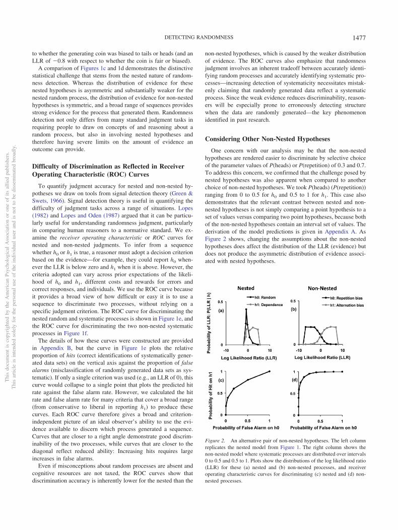
A comparison of Figures 1c and 1d demonstrates the distinctivestatistical challenge that stems from the nested nature of random-ness detection. Whereas the distribution of evidence for thesenested hypotheses is asymmetric and substantially weaker for thenested random process, the distribution of evidence for non-nestedhypotheses is symmetric, and a broad range of sequences providesstrong evidence for the process that generated them. Randomnessdetection not only differs from many standard judgment tasks inrequiring people to draw on concepts of and reasoning about arandom process, but also in involving nested hypotheses andtherefore having severe limits on the amount of evidence anoutcome can provide.
Difficulty of Discrimination as Reflected in ReceiverOperating Characteristic (ROC) Curves
To quantify judgment accuracy for nested and non-nested hy-potheses we draw on tools from signal detection theory (Green &Swets, 1966). Signal detection theory is useful in quantifying thedifficulty of judgment tasks across a range of situations. Lopes(1982) and Lopes and Oden (1987) argued that it can be particu-larly useful for understanding randomness judgment, particularlyin comparing human reasoners to a normative standard. We ex-amine the receiver operating characteristic or ROC curves fornested and non-nested judgments. To infer from a sequencewhether h0 or h1 is true, a reasoner must adopt a decision criterionbased on the evidence—for example, they could report h0 when-ever the LLR is below zero and h1 when it is above. However, thecriteria adopted can vary across prior expectations of the likeli-hood of h0 and h1, different costs and rewards for errors andcorrect responses, and individuals. We use the ROC curve becauseit provides a broad view of how difficult or easy it is to use asequence to discriminate two processes, without relying on aspecific judgment criterion. The ROC curve for discriminating thenested random and systematic processes is shown in Figure 1e, andthe ROC curve for discriminating the two non-nested systematicprocesses in Figure 1f.
The details of how these curves were constructed are providedin Appendix B, but the curve in Figure 1e plots the relativeproportion of hits (correct identifications of systematically gener-ated data sets) on the vertical axis against the proportion of falsealarms (misclassification of randomly generated data sets as sys-tematic). If only a single criterion was used (e.g., an LLR of 0), thiscurve would collapse to a single point that plots the predicted hitrate against the false alarm rate. However, we calculated the hitrate and false alarm rate for many criteria that cover a broad range(from conservative to liberal in reporting h1) to produce thesecurves. Each ROC curve therefore gives a broad and criterion-independent picture of an ideal observer’s ability to use the evi-dence available to discern which process generated a sequence.Curves that are closer to a right angle demonstrate good discrim-inability of the two processes, while curves that are closer to thediagonal reflect reduced ability: Increasing hits requires largeincreases in false alarms.
Even if misconceptions about random processes are absent andcognitive resources are not taxed, the ROC curves show thatdiscrimination accuracy is inherently lower for the nested than the
non-nested hypotheses, which is caused by the weaker distributionof evidence. The ROC curves also emphasize that randomnessjudgment involves an inherent tradeoff between accurately identi-fying random processes and accurately identifying systematic pro-cesses—increasing detection of systematicity necessitates mistak-enly claiming that randomly generated data reflect a systematicprocess. Since the weak evidence reduces discriminability, reason-ers will be especially prone to erroneously detecting structurewhen the data are randomly generated—the key phenomenonidentified in past research.
Considering Other Non-Nested Hypotheses
One concern with our analysis may be that the non-nestedhypotheses are rendered easier to discriminate by selective choiceof the parameter values of P(heads) or P(repetition) of 0.3 and 0.7.To address this concern, we confirmed that the challenge posed bynested hypotheses was also apparent when compared to anotherchoice of non-nested hypotheses. We took P(heads) (P(repetition))ranging from 0 to 0.5 for h0 and 0.5 to 1 for h1. This case alsodemonstrates that the relevant contrast between nested and non-nested hypotheses is not simply comparing a point hypothesis to aset of values versus comparing two point hypotheses, because bothof the non-nested hypotheses contain an interval set of values. Thederivation of the model predictions is given in Appendix A. AsFigure 2 shows, changing the assumptions about the non-nestedhypotheses does affect the distribution of the LLR (evidence) butdoes not produce the asymmetric distribution of evidence associ-ated with nested hypotheses.
Figure 2. An alternative pair of non-nested hypotheses. The left columnreplicates the nested model from Figure 1. The right column shows thenon-nested model where systematic processes are distributed over intervals0 to 0.5 and 0.5 to 1. Plots show the distributions of the log likelihood ratio(LLR) for these (a) nested and (b) non-nested processes, and receiveroperating characteristic curves for discriminating (c) nested and (d) non-nested processes.
Thi
sdo
cum
ent
isco
pyri
ghte
dby
the
Am
eric
anPs
ycho
logi
cal
Ass
ocia
tion
oron
eof
itsal
lied
publ
ishe
rs.
Thi
sar
ticle
isin
tend
edso
lely
for
the
pers
onal
use
ofth
ein
divi
dual
user
and
isno
tto
bedi
ssem
inat
edbr
oadl
y.
1477DETECTING RANDOMNESS
Summary
The ideal observer analysis elucidates the precise nature of theinherent statistical difficulty in detecting randomness—it is anested hypothesis. Discriminating a random process (like P(heads)or P(repetition) of 0.5) from a systematic process (P(heads) orP(repetition) has another value between 0 and 1) is a difficultstatistical task because randomly generated data are also reason-ably likely to have come from systematic processes. Calculatingthe distribution of the LLR of data sets generated by both kinds ofprocesses provides a quantitative measure of the evidence resultingfrom an observation, demonstrating that randomly generated datagive relatively weak evidence for a random process. The paucity ofthis evidence was clear in the comparison to the evidence that canbe provided for a systematic process, and to the evidence providedby data sets from non-nested hypotheses. ROC curves indicatedthat the information available in judging randomness was lowerthan for the other tasks, such that raising correct identifications ofsystematic process would necessitate higher false alarms in incor-rectly judging that randomly generated data set reflected a system-atic process.
Exploring the Source of Errors in HumanRandomness Judgments
Our nested hypothesis account provides a novel proposal forwhy people find detecting randomness difficult. But we needempirical evidence that people’s judgments are actually sensitiveto the statistical measures we present. Moreover, there is clearreason to believe people have misconceptions about randomnessand processing limitations, which may eliminate or overwhelm anyeffects of our statistical measures on judgment.
We conducted three experiments that investigated the extent towhich accuracy and errors depended on the statistical propertieshighlighted in our analysis—the log likelihood ratio, or quantity ofevidence available—versus whether people needed to reason aboutand represent a random process. Our analysis predicts that accu-racy should be primarily a function of the evidence provided by asequence (the LLR), which is highly dependent on whether thehypotheses under consideration are nested. Alternatively, the sta-tistical model we analyzed may fail to accurately capture theevidence available to people, or statistical considerations may playa minimal role if errors are driven largely by people’s difficultiesin conceptualizing and reasoning about randomness.
All three experiments compared the accuracy of judgments in anested condition—discriminating a random from a systematicallybiased process—to judgments in a non-nested condition—discrim-inating two systematic processes. Accuracy is predicted to belower in the nested condition, whether because of (1) people’slimitations in conceptualizing and reasoning about a random pro-cess, and/or (2) the low LLRs or weak evidence available for anested hypothesis—as predicted by our analysis. To evaluate thesepossibilities, we compared the nested and non-nested condition toa critical matched condition. The matched condition used the samejudgment task as the non-nested condition, but the same distribu-tion of evidence as the nested condition. Although people did notneed to reason about a random process, a model was used tostatistically equate the available evidence to that in the nestedcondition. The model’s predictions about the LLR were used to
choose the sequences in the matched condition so they providedexactly as much evidence for discriminating the non-nested hy-potheses as the sequences in the nested condition did for discrim-inating random from systematic processes.
If our nested hypothesis account correctly characterizes thestatistical difficulty people face in detecting randomness, thematched condition should have lower accuracy than the non-nestedcondition. If the model captures the difficulty of the task, thematched condition may even be as inaccurate as the nested. If themodel does not capture difficulty, or these considerations areminimal relevant to other factors, accuracy in the matched condi-tion should not differ from the non-nested and could even begreater. The model can also be evaluated by assessing how well theLLR—the model’s measure of evidence—predicts people’s accu-racy and reaction time in making judgments on particular data sets.The model predicts that judgments on sequences with small LLRs(not very diagnostic) should be near chance and have slow reactiontimes, with the opposite pattern for sequences with large LLRs.
While all the experiments followed this basic logic, the task inExperiments 1 and 2 was deciding if a coin was random (heads andtails equally likely) or biased toward heads/tails. Experiment 3extended the model to the more complex task of deciding whethera coin was random (independent of previous coin flips—repeti-tions or alternations equally likely) or biased toward repetition/alternation, allowing us to investigate whether the nested hypoth-esis account predicts people’s judgment errors even in situations inwhich people have known misconceptions about randomness.
Experiment 1: Judging Randomness in theFrequency of Events
As mentioned above, Experiment 1 examined judgments aboutwhether a coin was random (equally likely to produce heads ortails) or systematically biased (toward heads, or toward tails). Itinvestigated whether our nested hypothesis account provided anaccurate characterization of the source of errors in people’s ran-domness judgments. In the non-nested condition, participantsjudged whether sequences were biased toward heads or tails for 50sequences that covered a range of evidence characteristic of biasedcoins. In the nested condition, participants judged whether a coinwas fair (random) or biased for 50 sequences that covered a rangeof evidence characteristic of fair and biased coins. In the matchedcondition, judgments concerned whether a coin was biased towardheads or tails, but the LLR (our model’s measure of the evidencea sequence provided) was used to select 50 sequences that pro-vided exactly as much evidence for a bias to heads/tails as the 50in the nested condition provided for a fair/biased coin. Althoughthe tasks differed, the distribution of LLRs was thus the same inthe nested and matched conditions.
Method
Participants. Participants were 120 undergraduate students(40 in each of three conditions), participating for course credit.
Materials. The 50 sequences in the nested and non-nestedcondition were chosen to span a range of sequences that wouldbe generated under the nested and non-nested hypotheses. Table1 shows the distribution of LLRs for the sequences in eachcondition, as well as example sequences in each range of LLRs,
Thi
sdo
cum
ent
isco
pyri
ghte
dby
the
Am
eric
anPs
ycho
logi
cal
Ass
ocia
tion
oron
eof
itsal
lied
publ
ishe
rs.
Thi
sar
ticle
isin
tend
edso
lely
for
the
pers
onal
use
ofth
ein
divi
dual
user
and
isno
tto
bedi
ssem
inat
edbr
oadl
y.
1478 WILLIAMS AND GRIFFITHS
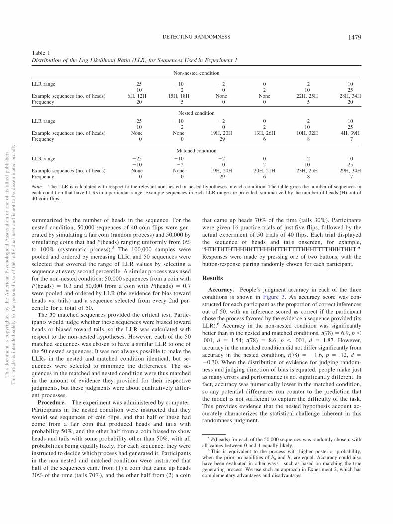
summarized by the number of heads in the sequence. For thenested condition, 50,000 sequences of 40 coin flips were gen-erated by simulating a fair coin (random process) and 50,000 bysimulating coins that had P(heads) ranging uniformly from 0%to 100% (systematic process).5 The 100,000 samples werepooled and ordered by increasing LLR, and 50 sequences wereselected that covered the range of LLR values by selecting asequence at every second percentile. A similar process was usedfor the non-nested condition: 50,000 sequences from a coin withP(heads) � 0.3 and 50,000 from a coin with P(heads) � 0.7were pooled and ordered by LLR (the evidence for bias towardheads vs. tails) and a sequence selected from every 2nd per-centile for a total of 50.
The 50 matched sequences provided the critical test. Partic-ipants would judge whether these sequences were biased towardheads or biased toward tails, so the LLR was calculated withrespect to the non-nested hypotheses. However, each of the 50matched sequences was chosen to have a similar LLR to one ofthe 50 nested sequences. It was not always possible to make theLLRs in the nested and matched condition identical, but se-quences were selected to minimize the differences. The se-quences in the matched and nested condition were thus matchedin the amount of evidence they provided for their respectivejudgments, but these judgments were about qualitatively differ-ent processes.
Procedure. The experiment was administered by computer.Participants in the nested condition were instructed that theywould see sequences of coin flips, and that half of these hadcome from a fair coin that produced heads and tails withprobability 50%, and the other half from a coin biased to showheads and tails with some probability other than 50%, with allprobabilities being equally likely. For each sequence, they wereinstructed to decide which process had generated it. Participantsin the non-nested and matched condition were instructed thathalf of the sequences came from (1) a coin that came up heads30% of the time (tails 70%), and the other half from (2) a coin
that came up heads 70% of the time (tails 30%). Participantswere given 16 practice trials of just five flips, followed by theactual experiment of 50 trials of 40 flips. Each trial displayedthe sequence of heads and tails onscreen, for example,“HTHTHTHTHHHHTTHHHHTTHTTTTHHHTTTTHHHTHHT.”Responses were made by pressing one of two buttons, with thebutton-response pairing randomly chosen for each participant.
Results
Accuracy. People’s judgment accuracy in each of the threeconditions is shown in Figure 3. An accuracy score was con-structed for each participant as the proportion of correct inferencesout of 50, with an inference scored as correct if the participantchose the process favored by the evidence a sequence provided (itsLLR).6 Accuracy in the non-nested condition was significantlybetter than in the nested and matched conditions, t(78) � 6.9, p �.001, d � 1.54; t(78) � 8.6, p � .001, d � 1.87. However,accuracy in the matched condition did not differ significantly fromaccuracy in the nested condition, t(78) � �1.6, p � .12, d ��0.30. When the distribution of evidence for judging random-ness and judging direction of bias is equated, people make justas many errors and performance is not significantly different. Infact, accuracy was numerically lower in the matched condition,so any potential differences run counter to the prediction thatthe model is not sufficient to capture the difficulty of the task.This provides evidence that the nested hypothesis account ac-curately characterizes the statistical challenge inherent in thisrandomness judgment.
5 P(heads) for each of the 50,000 sequences was randomly chosen, withall values between 0 and 1 equally likely.
6 This is equivalent to the process with higher posterior probability,when the prior probabilities of h0 and h1 are equal. Accuracy could alsohave been evaluated in other ways—such as based on matching the truegenerating process. We use such an approach in Experiment 2, which hascomplementary advantages and disadvantages.
Table 1Distribution of the Log Likelihood Ratio (LLR) for Sequences Used in Experiment 1
Non-nested condition
LLR range �25 �10 �2 0 2 10�10 �2 0 2 10 25
Example sequences (no. of heads) 6H, 12H 15H, 18H None None 22H, 25H 28H, 34HFrequency 20 5 0 0 5 20
Nested condition
LLR range �25 �10 �2 0 2 10�10 �2 0 2 10 25
Example sequences (no. of heads) None None 19H, 20H 13H, 26H 10H, 32H 4H, 39HFrequency 0 0 29 6 8 7
Matched condition
LLR range �25 �10 �2 0 2 10�10 �2 0 2 10 25
Example sequences (no. of heads) None None 19H, 20H 20H, 21H 23H, 25H 29H, 34HFrequency 0 0 29 6 8 7
Note. The LLR is calculated with respect to the relevant non-nested or nested hypotheses in each condition. The table gives the number of sequences ineach condition that have LLRs in a particular range. Example sequences in each LLR range are provided, summarized by the number of heads (H) out of40 coin flips.
Thi
sdo
cum
ent
isco
pyri
ghte
dby
the
Am
eric
anPs
ycho
logi
cal
Ass
ocia
tion
oron
eof
itsal
lied
publ
ishe
rs.
Thi
sar
ticle
isin
tend
edso
lely
for
the
pers
onal
use
ofth
ein
divi
dual
user
and
isno
tto
bedi
ssem
inat
edbr
oadl
y.
1479DETECTING RANDOMNESS

Model predictions: Degree of belief. Figure 4 shows theproportion of people choosing h1 for each of the 50 sequences, aswell as the posterior probability of h1 according to the model’sanalysis of the judgment—the precise degree of belief in h1 that iswarranted by the evidence the data provide.7 The sequences areordered from left to right by increasing LLR. The key patternillustrated in Figure 4 is that there is a striking quantitative corre-spondence between the proportion of people who choose a processand the model’s degree of belief in that process, according to theLLR of the data set. The correlations for the non-nested, nested,and matched conditions are, respectively, r(48) � .99, .94, and .92,providing compelling evidence that the model accurately capturesthe statistical difficulty in detecting randomness.
Model predictions: Reaction time. All reaction time analy-ses were carried out on data that were first scaled for outliers(reaction times greater than 10 s were replaced by a value of 10 s).Reaction time data confirm the pattern of difficulty in judgments:People were faster to make judgments in the non-nested conditionthan either the nested condition, t(78) � 2.5, p � .02, d � 0.56, ormatched condition, t(78) � 2.7, p � .01, d � 0.60, althoughreaction time for the matched condition was not significantlydifferent from the nested condition, t(78) � �0.33, p � .74, d ��0.07.
Reaction time was also analyzed as a function of individualsequences (or rather, their LLRs) to obtain detailed model predic-tions. There was a clear linear relationship between the time peopleneeded to make a judgment about a sequence and the magnitude ofthe evidence that sequence provided (the size of the LLR). Thecorrelations between the time to make an inference from a se-quence and the absolute value of the LLR of the sequence werer(48) � �.82 (non-nested), �.84 (nested), and �.75 (matched).The smaller the magnitude of the LLR, the longer the time to makea judgment, the larger the LLR, the quicker an inference was made.The close match between data and model illustrates that thesequences which provide only weak evidence are the sequencesthat people find inherently difficult to evaluate and spend moretime processing.
Discussion
Experiment 1 provided evidence for the nested hypothesis ac-count. Although judgments about a random process (fair coin)were less accurate than similar task judgments about non-nestedhypotheses (head/tail bias), this was due to the weak evidence
available rather than people’s erroneous intuitions about random-ness. The matched condition required judgments about non-nestedhypotheses, eliminating the role of biases about randomness inerroneous judgments. But it also equated the amount of evidencesequences provided to the evidence available in the nested condi-tion. This eliminated the significant differences, so that the nestedand matched conditions were equally accurate. These results sug-gest that judgments about randomness are more inaccurate thanjudgments about two kinds of systematic processes not only be-cause they involve reasoning about randomness, but because judg-ments about randomness are judgments about nested hypotheses.
Across a range of sequences, the proportion of people whojudged a random process to be present closely tracked the rationaldegree of belief an ideal observer would possess based on thestatistical evidence available. There was also a close correspon-dence between the strength of evidence and the difficulty ofmaking a judgment, as measured by reaction time. The resultssuggest that the assumptions of the model about how processes arementally represented and related to data provides a good accountof participants’ difficulty and errors in judging randomness, byclosely capturing the uncertainty in the evidence available. Inparticular, the high correlations between model and data suggestthat people are very sensitive to the evidence a sequence providesfor a process and are good at judging how likely it is that aparticular process generated a sequence.
The proportion of people selecting a particular process corre-sponded closely to the posterior probability of this process. Thiskind of “probability matching” might seem inconsistent with theassumption of rationality behind our model: The rational actionshould be to deterministically select the process that has highestposterior probability. There are several possible explanations forwhy this is not the case. Even if the evidence available is constantacross participants, the particular criterion each uses for a judg-
7 The model assumes that h0 (a random process) and h1 (a systematicprocess) are equally likely a priori (the instructions provided to participantsalso indicate that this is the case), and so the posterior probability depends
only on the LLR: It is equal to1
1�e�LLR.Figure 3. Judgment accuracy as a function of task and evidence inExperiment 1. Error bars represent one standard error.
Figure 4. Results of Experiment 1, showing the proportion of peoplereporting that a sequence was generated by h1 and the posterior probabilityof h1 for that sequence. h1 represented a systematically biased process forthe nested condition and a bias to heads for the symmetric and matched.Sequences are ordered by increasing evidence for h1. LLR � log likelihoodratio.
Thi
sdo
cum
ent
isco
pyri
ghte
dby
the
Am
eric
anPs
ycho
logi
cal
Ass
ocia
tion
oron
eof
itsal
lied
publ
ishe
rs.
Thi
sar
ticle
isin
tend
edso
lely
for
the
pers
onal
use
ofth
ein
divi
dual
user
and
isno
tto
bedi
ssem
inat
edbr
oadl
y.
1480 WILLIAMS AND GRIFFITHS
ment may vary. Also, participants do not necessarily have directaccess to a quantitative measure of the evidence in a stimulus, butmay process a noisy function of this evidence. As the evidencebecomes stronger, both an ideal observer’s confidence and partic-ipants’ correct responses increase, because they are sensitive to thesame statistical information, even if different procedures or pro-cesses map this information to a particular judgment. Vulkan(2000) and Shanks, Tunney, and McCarthy (2002) have providedfurther discussion of issues relating to this kind of probabilitymatching.
Experiment 2: Dissociating Random Processes andNested Hypotheses
One reason Experiment 1 provided support for our nested hy-pothesis account was that the nested and matched conditions wereequally accurate despite differing in whether participants had toreason about randomness. But a drawback of this difference is thatthe comparison of the nested condition to the matched (and non-nested) condition does not isolate being nested as a critical feature,as opposed to involving reasoning about randomness. Experiment2 addressed this issue by extending Experiment 1 in two ways.
The first was that the nested judgment was compared to ajudgment that was both non-nested and required reasoning about arandom process. This random non-nested condition required dis-criminating a random coin (P(heads) � 0.5) from a biased cointhat produced heads 80% of the time. Although this conditionalso requires detecting a random process, the nested modelpredicts a more informative distribution of evidence and higheraccuracy since the hypothesis of randomness is not nestedwithin the alternative hypothesis. The matched condition wassimilarly adapted to provide a more direct comparison to thenested condition by using the random non-nested judgmenttask, but statistically matching the evidence to that in the nestedcondition, which we now label the random nested condition.
The second extension was that we included two conditions thatallowed us to independently manipulate whether participants madejudgments about random (vs. only systematic) processes, andwhether the judgments were nested (vs. non-nested). The system-atic non-nested condition did not require reasoning about a randomprocess, but was chosen to be statistically similar to the randomnon-nested condition. It required discrimination of a process withP(heads) � 0.4 from one with P(heads) � 0.7. The systematicnested condition was statistically similar to the random nestedcondition. It required evaluating whether a sequence was generatedby a systematically biased coin with P(heads) � 0.4 or a biasedcoin with P(heads) between 0 and 1.
The result of these two extensions is a 2 (judgment: requires vs.does not require consideration of a random process) � 2 (statisticalstructure: nested vs. non-nested) design. Our nested hypothesisaccount predicts a main effect of statistical structure—where ac-curacy is lower for nested than non-nested hypotheses—but noeffect of whether the judgment involves consideration of a randomprocess. Alternatively, if the involvement of random processes iswhat makes a task hard, accuracy should be lower wheneverpeople have to use their concept of randomness or apply a heuristicin evaluating a random process. Finally, if the statistical structureof the task is irrelevant, we should see no difference between thenested and non-nested judgments.
Two further changes were made to complement Experiment 1.To more directly target intuitions about randomness, participantsin the random conditions were instructed to judge whether asequence reflected a random coin. Experiment 1 framed the task asidentifying whether the coin had a 50% probability of heads, whichwas logically equivalent but may not have directly tapped intu-itions about randomness. Also, Experiment 1 selected sequenceswith a broad range of LLRs and so had to use the ideal observermodel to assess accuracy. Experiment 2 chose the sequences toreflect the distribution associated with each of the generatingprocesses, keeping track of which sequences were generated fromeach process so that this information could be used in scoringresponses. Using both of these methods for selecting sequencesand scoring accuracy ensures that our findings are not an artifact ofany particular method.
Method
Participants. Participants were 90 undergraduate studentswho participated for course credit and 110 members of the generalpublic recruited through Amazon Mechanical Turk (http://www.mturk.com) who received a small amount of financial compensa-tion. Participants were randomly allocated to condition, resultingin 40 participants in each of five conditions.
Materials. The systematic non-nested (P(heads) � 0.4 vs.0.7), random non-nested (P(heads) � 0.5 vs. 0.8), systematicnested (P(heads) � 0.4 vs. [0, 1]), and random nested (P(heads) �0.5 vs. [0, 1]) conditions each presented 50 sequences of 40 coinflips, 25 from each process. Sequences were selected so that theirfrequencies reflected their probability under the correspondingprocess. For example, if P(heads) � 0.5, the probability of asequence with 20 heads is 0.125, and so there were three sequenceswith 20 heads (0.125 � 25 � 3.125). For the matched condition,the 50 sequences were selected so that the LLRs with respect to therandom non-nested judgment (P(heads) of 0.5 vs. 0.8) were assimilar as possible to the LLRs in the random nested condition.
Procedure. Participants were informed that they would seesequences of heads and tails that were generated by differentprocesses and that they would judge what the generating processwas. For each condition, they were informed what the relevant pro-cesses were and told that half of the coins came from each process.For example, in the random nested condition, they were told that halfof the sequences came from a coin that is random—has 50% prob-ability of heads—and half from a coin that has an 80% probability ofheads. Each trial displayed the sequence onscreen, for example,“HHTHTHTHTHHHHTTHHHHTTHTTTTHHHTTTTHHHTHHT.”The order of the flips in a sequence was randomized on eachpresentation. Responses were made on the keyboard. To familiar-ize participants with the task, they had a practice phase of makingjudgments about 16 sequences of just five flips. The actual exper-iment required judgments for 50 sequences of 20 flips.
Results and Discussion
Accuracy was calculated in two ways. First, as in Experiment 1,an inference was scored as correct if the participant chose theprocess favored by the evidence a sequence provided (its LLR).Second, an inference was scored as correct if it corresponded to theprocess whose distribution was used to generate the sequence.
Thi
sdo
cum
ent
isco
pyri
ghte
dby
the
Am
eric
anPs
ycho
logi
cal
Ass
ocia
tion
oron
eof
itsal
lied
publ
ishe
rs.
Thi
sar
ticle
isin
tend
edso
lely
for
the
pers
onal
use
ofth
ein
divi
dual
user
and
isno
tto
bedi
ssem
inat
edbr
oadl
y.
1481DETECTING RANDOMNESS
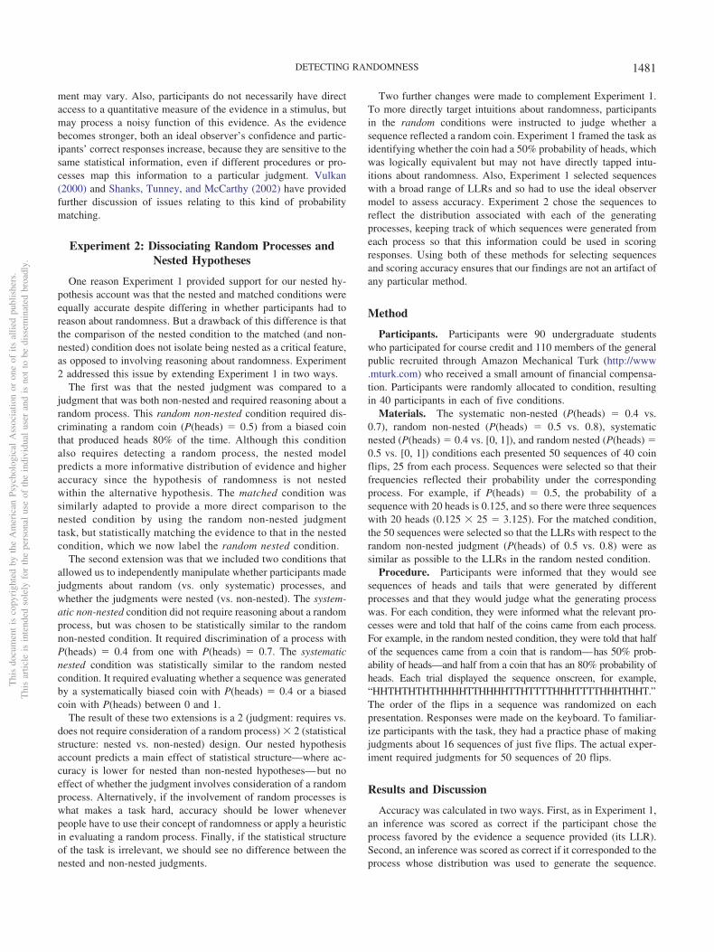
Both of these measures gave the same pattern of results, and to beconsistent throughout the article, we report the first. Figure 5shows accuracy for all five conditions: systematic non-nested,random non-nested, systematic nested, random nested, andmatched. Figure 6 shows the proportion of people who chose h1 foreach of the 50 sequences, along with the model predictions—theposterior probability of h1 for each of those sequences.
Comparison of random non-nested, random nested, andmatched judgments. Although both conditions involved a judg-ment about a random process, accuracy was significantly lower inthe random nested condition than the random non-nested condi-tion, t(78) � �4.67, p � .001, d � 1.04. This reflects theparticular challenge of discriminating nested hypotheses. To testwhether this was due to weaker evidence in the random nestedcondition, the matched condition judged whether a sequence wasfrom a coin with P(heads) � 0.5 or 0.8, but only for sequenceswith LLRs matched to those in the random nested condition.Accuracy in the matched condition was also significantly lowerthan the random non-nested condition, t(78) � �4.61, p � .001,d � 1.03, but did not differ significantly from the random nestedcondition, t(78) � 0.09, p � .93, d � 0.02. This replicates thefinding from Experiment 1 that a weaker distribution of evidencewas responsible for errors in randomness judgment, which isunderscored by the better accuracy in reasoning about a randomprocess when it was not nested.
Judgment as a function of whether a process is randomand/or nested. Accuracy in the systematic non-nested, randomnon-nested, systematic nested, and random nested conditions wasanalyzed in a 2 (random vs. systematic) � 2 (nested vs. non-nested) analysis of variance (ANOVA). Judgments that involvednested hypotheses were significantly less accurate than judgmentsabout non-nested hypotheses, F(1, 195) � 65.22, p � .001. How-ever, there was no effect of whether a judgment involved reasoningabout a random or systematic process, F(1, 195) � 1, p � .94.These results support our nested hypothesis account of errors inrandomness judgment, with whether hypotheses were nested hav-ing a bigger effect than whether people had to reason about arandom process.
The interaction between the two factors in the ANOVA was notsignificant, F(1, 195) � 3.56, p � .06. Accuracy in the systematicnon-nested condition did not differ significantly from accuracy in
the random non-nested condition, t(78) � �0.28, p � .78, d ��0.06. Accuracy in the systematic nested condition did not differsignificantly from the random non-nested condition, t(78) � 1.79,p � .08, d � 0.4, and if anything the trend was for it to be lower.
The proportion of people reporting that a particular processgenerated a sequence was closely predicted by the posterior prob-ability of that process under the model. The correlations for eachcondition were systematic non-nested, r(48) � .96; systematicnested, r(48) � .84; random non-nested, r(48) � .95; randomnested, r(48) � .84; and matched, r(48) � .86. Reaction time datawere not analyzed because many participants conducted the ex-periment online, preventing accurate measurement of reactiontimes for all participants. Across a range of tasks, the ideal ob-server analysis provided a compelling account of people’s judg-ments, in terms of the evidence available in evaluating nested,random, and systematic processes.
Experiment 3A: Evaluating Randomness VersusSequential Dependence
Experiments 1 and 2 provided support for our nested hypothesisaccount, showing that people’s errors in detecting randomness areat least partially due to the statistical structure of the task. Exper-iment 3 was designed to test the predictions of our account in adifferent kind of randomness judgment. The task was judgingwhether successive coin flips were random in being independent ofeach other or exhibited systematic sequential dependency, with theprobability of repetition (and alternation) being other than 50%.The conceptions of randomness and reasoning strategies peopleuse in this task may differ from Experiments 1 and 2, but the taskstill shares the key statistical property of evaluating nested hypoth-
Figure 5. Judgment accuracy as a function of task and evidence inExperiment 2. Error bars represent one standard error.
Figure 6. Results of Experiment 2, showing the proportion of peoplereporting that a sequence was generated by h1 and posterior probability ofh1 under the model. h1 represented a systematically biased process for thenested conditions and a bias to heads for the symmetric and matchedconditions. Sequences are ordered by increasing evidence for h1. LLR �log likelihood ratio.
Thi
sdo
cum
ent
isco
pyri
ghte
dby
the
Am
eric
anPs
ycho
logi
cal
Ass
ocia
tion
oron
eof
itsal
lied
publ
ishe
rs.
Thi
sar
ticle
isin
tend
edso
lely
for
the
pers
onal
use
ofth
ein
divi
dual
user
and
isno
tto
bedi
ssem
inat
edbr
oadl
y.
1482 WILLIAMS AND GRIFFITHS

eses. Extending our mathematical analysis to this task also pro-vides an opportunity to show how it can be used to integratestatistical inference with cognitive biases, as there is ample evi-dence that people have misleading intuitions about sequentialdependency. Specifically, people demonstrate an alternation bias,believing that sequences with many alternations (e.g., alternatingfrom heads to tails) are more random than sequences with manyrepetitions (e.g., repeating heads or tails), and that repetitions aremore likely to reflect systematic processes (Bar-Hillel & Wage-naar, 1993; Falk & Konold, 1997).
People’s alternation bias is illustrated in Figure 7 (data fromFalk & Konold, 1997, Experiment 3). Apparent randomness rat-ings are plotted as a function of how likely the sequence is toalternate. The alternation bias is obvious when human judgmentsare compared to the model that we used in the mathematicalanalysis presented earlier in the article. From this point on, welabel this the uniform model because it assumes that all systematicprocesses are equally likely. The model ratings of randomnessshown in Figure 7 were computed by evaluating the LLR asequence provides and scaling it to the same range as humanjudgments. Although the uniform model captures the generaltrend, it fails to capture human ratings of alternating sequences asmore random than repeating sequences.
To test whether the statistical structure of the task makes acontribution to errors above and beyond documented cognitivebiases, we defined a new biased model that incorporates an alter-nation bias. This model shows how an ideal observer may entertainmisleading hypotheses that do not match the structure of the world,but still be sensitive to the evidence that observations provide forthose hypotheses. The biased model replaced the assumption thatall systematic processes were equally likely with an assumptionthat systematic processes were more likely to be repeating than tobe alternating. As we consider in the General Discussion, differentapproaches could be taken, but our goal was simply to capture thebias accurately enough to test the key prediction about nestedhypotheses. The assumption that systematic processes are morelikely to be repeating than alternating was captured by defining abeta distribution rather than a uniform distribution over P(repeti-tion). The mathematical details of how the parameters of thisdistribution were selected are presented in Appendices A and C,but in Experiment 3A, they were chosen to capture the magnitudeof the alternation bias in data from Falk and Konold’s (1997)
Experiment 3. In Experiment 3B, the parameters were then chosento capture the alternation bias demonstrated by participants inExperiment 3A, so that our findings would not be an artifact of aspecific parameter choice. Figure 7 shows that the biased modelbetter captures people’s judgments about the relative randomnessof repetitions and alternations.
Even when the alternation bias is incorporated into the model,the random process is still nested in a range of systematic pro-cesses. Replicating our ideal observer analysis with the biasedinstead of uniform model produces the same results: Randomlygenerated data have weaker LLRs and should lead to more errors,in addition to those caused by the alternation bias. As in previousexperiments, nested, matched, and non-nested conditions werecompared. However, in contrast to previous experiments, partici-pants in the nested condition were simply informed that the coincame from a “random” or “non-random” process and were givenno information about these processes. Because the judgment reliesonly on people’s intuitions about what “random” and “non-random” means, this provided a strong test of whether our nestedhypothesis account truly characterizes the challenges in humanreasoning about randomness.
Method
Participants. Participants were 120 undergraduate students(40 in each of three conditions) who received course credit.
Materials. Sequences were selected using a similar method toExperiment 1. However, the number of flips was reduced to 20,and all sequences used exactly 10 heads and 10 tails, consistentwith previous research (Falk & Konold, 1997).
For nested sequences, 50,000 sequences were generated bysimulating a random coin with independent flips (P(repetition) �0.5). Another 50,000 sequences were generated by simulating acoin that was biased to repetition or alternation (P(repetition)ranged uniformly from 0 to 1).8 The LLR of each sequence wascomputed under the biased model, all sequences were pooled andordered by increasing LLR, and 50 sequences were selected bychoosing one at each 2nd percentile.
For non-nested sequences, 50,000 sequences were generated bysimulating a coin biased to repeat (P(repetition) ranged uniformlyfrom 0.5 to 1) and 50,000 by simulating a coin biased to alternate(P(repetition) ranged uniformly from 0 to 0.5). The LLR of eachsequence was computed (relative to the non-nested hypotheses ofa bias to repetition or alternation), the sequences were pooled andordered, and 50 sequences that spanned the range of LLRs wereselected.
For matched sequences, the LLRs in the nested condition wereused to select two sets of 25 matched sequences. In matching theLLRs of the first set of 25 matched sequences, positive LLRsprovided evidence for repetition, while in the second set, positiveLLRs provided evidence for alternation. The distribution of theLLRs for the nested sequences was not symmetric around zero
8 Although the model assumes the representation of a systematic processis biased toward repetitions, the generation of systematic sequences did notreflect this bias to ensure that the sequences would be representative ofactual random and systematic processes. However, the biased model wasused to compute the LLR and determine how much evidence a sequenceprovided for a random process.
Figure 7. Human and model randomness ratings for binary sequencespresented by Falk and Konold (1997). The uniform model assumes thatrepetitions and alternations are judged equally systematic, whereas thebiased model assumes that repetitions are more systematic than alterna-tions.
Thi
sdo
cum
ent
isco
pyri
ghte
dby
the
Am
eric
anPs
ycho
logi
cal
Ass
ocia
tion
oron
eof
itsal
lied
publ
ishe
rs.
Thi
sar
ticle
isin
tend
edso
lely
for
the
pers
onal
use
ofth
ein
divi
dual
user
and
isno
tto
bedi
ssem
inat
edbr
oadl
y.
1483DETECTING RANDOMNESS

(ranging from �0.8 to �4.0), so this control ensured that thematched sequences provided the same overall amount of evidencefor repetition and alternation, guarding against possible asymme-tries in judgment. The 25 LLRs used in the matched condition stillspanned the full range of evidence: They were obtained by aver-aging every two successive LLRs in the nested condition (i.e., theLLRs of the 1st and 2nd sequences, 3rd and 4th, and so on up tothe 49th and 50th).
Procedure. Participants were informed that they would seesequences of heads and tails that were generated by differentcomputer simulated processes, and that their job would be to inferwhat process was responsible for generating each sequence. In thenon-nested and matched conditions, participants were instructedthat about half the sequences were generated by computer simu-lations of a coin that tends to repeat its flips (go from heads toheads or tails to tails) and the other half by simulations of a cointhat tends to change its flips (go from heads to tails or tails toheads). In the nested condition, participants were simply told thathalf the sequences were generated by computer simulations of arandom process and that half were generated by simulations of anon-random process. Participants received a practice phase wherethey made judgments about 16 sequences of just five flips, tofamiliarize them with the task. They then provided judgments for50 sequences of 20 flips. Each trial displayed the sequence ofheads and tails onscreen.
Results and Discussion
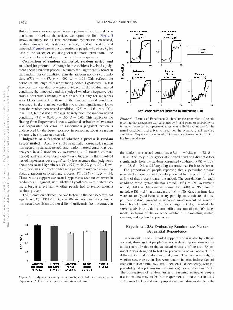
Accuracy for each condition is shown in Figure 8. As in Exper-iment 1, accuracy was significantly higher in the non-nested con-dition than the nested and matched conditions, t(78) � 6.61, p �.0001, d � 1.48; t(78) � 7.48, p � .0001, d � 1.67. However,there was no significant difference between the matched andnested conditions, t(78) � �1.35, p � .18, d � �0.3. Once theevidence that the sequence provides was equated to that of se-quences in the nested condition, the difficulty of judging whethera sequence was biased to alternate and repeat was not significantlydifferent from judging whether it was random or not. People facea double challenge in randomness judgments. Not only do mis-conceptions like the alternation bias reduce accuracy, but theinherent statistical limitations on the evidence available for anested random process also generate errors.
Figure 9 shows the posterior probability of h1 under the modeland the proportion of participants choosing h1, across all threeconditions. The proportion of participants choosing the hypothesis
closely tracked the degree of an optimal reasoner’s belief in thathypothesis. The correlations between the model predictions andhuman judgments were r(48) � .96 (non-nested), .87 (nested), and.79 (matched). People’s uncertainty and errors closely tracked therational degree of belief a reasoner should have based on theevidence a sequence provided. This is particularly noteworthybecause people were not told the nature of the random and sys-tematic processes and had to rely on their intuitions about “ran-dom” and “non-random” processes. There were no significantdifferences across conditions in the time to make judgments aboutsequences (all ps � 0.64; all ds � 0.10). The correlations betweenthe absolute value of the LLR and reaction times were r(48) ��.52 (non-nested), �.68 (nested), and �.23 (matched). Reactiontime may have been less informative because the range of LLRswas smaller than previous experiments.
Experiment 3B: Gaining a Closer Match toHuman Biases
Experiment 3A assumed that the alternation bias was similar tothat in Falk and Konold’s (1997) experiment, but these populationsand tasks may differ in significant ways. An informative compar-ison relies on the model representing similar hypotheses to peoplein a particular task. Our goal in Experiment 3B was to ensure thatthe results were not dependent on the particular model and param-eters used to capture the alternation bias in Experiment 3A. Just asExperiment 3A constructed a biased model to account for thealternation bias in Falk and Konold’s data, Experiment 3B repli-cated Experiment 3A using a model constructed to account for thealternation bias shown by participants in Experiment 3A by infer-ring the parameters that capture the randomness judgments made
Figure 9. Experiments 3A (top three panels) and 3B (bottom two panels):Proportion of people reporting that a sequence was generated by h1, andposterior probability of h1 under the model. h1 represented a sequentiallydependent process biased to repeat or alternate for the nested condition, anda bias to repeat flips for the symmetric and matched conditions. Sequencesare ordered by increasing evidence for h1. LLR � log likelihood ratio.
Figure 8. Judgment accuracy as a function of task and evidence inExperiment 3A. Error bars represent one standard error.
Thi
sdo
cum
ent
isco
pyri
ghte
dby
the
Am
eric
anPs
ycho
logi
cal
Ass
ocia
tion
oron
eof
itsal
lied
publ
ishe
rs.
Thi
sar
ticle
isin
tend
edso
lely
for
the
pers
onal
use
ofth
ein
divi
dual
user
and
isno
tto
bedi
ssem
inat
edbr
oadl
y.
1484 WILLIAMS AND GRIFFITHS
by these participants. The same procedure was used as in Exper-iment 3A, and the details are reported in Appendix C. While thenew parameters differed from those in Experiment 3A, the size ofthe alternation bias was similar to that found by Falk and Konold.Changing the model parameters did not influence the non-nestedcondition, so only the nested and matched conditions were repli-cated.
Method
Participants. Participants were 80 undergraduate students (40in each condition) who received course credit.
Materials. The procedure used to generate sequences wasidentical to that of Experiment 2, except that new parameters wereused for the biased model.
Procedure. The procedure was identical to Experiment 2.
Results and Discussion
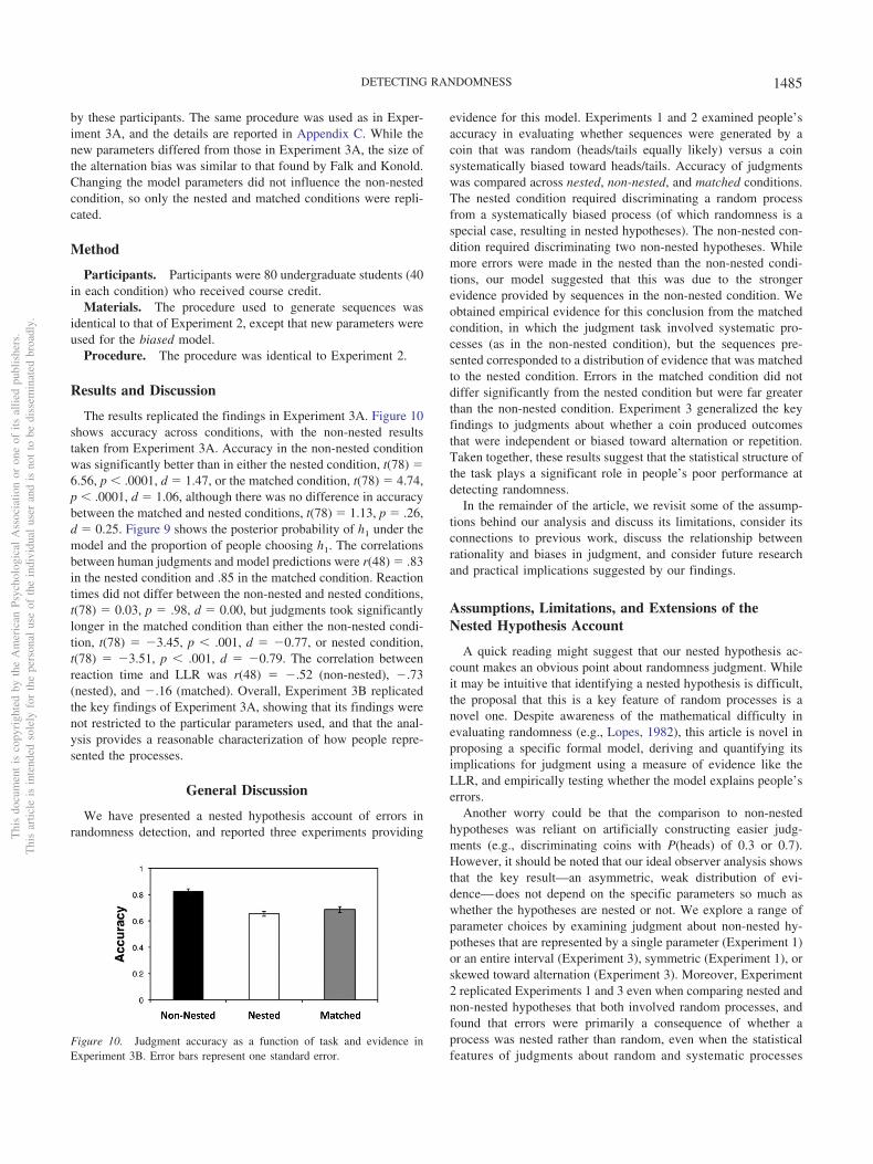
The results replicated the findings in Experiment 3A. Figure 10shows accuracy across conditions, with the non-nested resultstaken from Experiment 3A. Accuracy in the non-nested conditionwas significantly better than in either the nested condition, t(78) �6.56, p � .0001, d � 1.47, or the matched condition, t(78) � 4.74,p � .0001, d � 1.06, although there was no difference in accuracybetween the matched and nested conditions, t(78) � 1.13, p � .26,d � 0.25. Figure 9 shows the posterior probability of h1 under themodel and the proportion of people choosing h1. The correlationsbetween human judgments and model predictions were r(48) � .83in the nested condition and .85 in the matched condition. Reactiontimes did not differ between the non-nested and nested conditions,t(78) � 0.03, p � .98, d � 0.00, but judgments took significantlylonger in the matched condition than either the non-nested condi-tion, t(78) � �3.45, p � .001, d � �0.77, or nested condition,t(78) � �3.51, p � .001, d � �0.79. The correlation betweenreaction time and LLR was r(48) � �.52 (non-nested), �.73(nested), and �.16 (matched). Overall, Experiment 3B replicatedthe key findings of Experiment 3A, showing that its findings werenot restricted to the particular parameters used, and that the anal-ysis provides a reasonable characterization of how people repre-sented the processes.
General Discussion
We have presented a nested hypothesis account of errors inrandomness detection, and reported three experiments providing
evidence for this model. Experiments 1 and 2 examined people’saccuracy in evaluating whether sequences were generated by acoin that was random (heads/tails equally likely) versus a coinsystematically biased toward heads/tails. Accuracy of judgmentswas compared across nested, non-nested, and matched conditions.The nested condition required discriminating a random processfrom a systematically biased process (of which randomness is aspecial case, resulting in nested hypotheses). The non-nested con-dition required discriminating two non-nested hypotheses. Whilemore errors were made in the nested than the non-nested condi-tions, our model suggested that this was due to the strongerevidence provided by sequences in the non-nested condition. Weobtained empirical evidence for this conclusion from the matchedcondition, in which the judgment task involved systematic pro-cesses (as in the non-nested condition), but the sequences pre-sented corresponded to a distribution of evidence that was matchedto the nested condition. Errors in the matched condition did notdiffer significantly from the nested condition but were far greaterthan the non-nested condition. Experiment 3 generalized the keyfindings to judgments about whether a coin produced outcomesthat were independent or biased toward alternation or repetition.Taken together, these results suggest that the statistical structure ofthe task plays a significant role in people’s poor performance atdetecting randomness.
In the remainder of the article, we revisit some of the assump-tions behind our analysis and discuss its limitations, consider itsconnections to previous work, discuss the relationship betweenrationality and biases in judgment, and consider future researchand practical implications suggested by our findings.
Assumptions, Limitations, and Extensions of theNested Hypothesis Account
A quick reading might suggest that our nested hypothesis ac-count makes an obvious point about randomness judgment. Whileit may be intuitive that identifying a nested hypothesis is difficult,the proposal that this is a key feature of random processes is anovel one. Despite awareness of the mathematical difficulty inevaluating randomness (e.g., Lopes, 1982), this article is novel inproposing a specific formal model, deriving and quantifying itsimplications for judgment using a measure of evidence like theLLR, and empirically testing whether the model explains people’serrors.
Another worry could be that the comparison to non-nestedhypotheses was reliant on artificially constructing easier judg-ments (e.g., discriminating coins with P(heads) of 0.3 or 0.7).However, it should be noted that our ideal observer analysis showsthat the key result—an asymmetric, weak distribution of evi-dence—does not depend on the specific parameters so much aswhether the hypotheses are nested or not. We explore a range ofparameter choices by examining judgment about non-nested hy-potheses that are represented by a single parameter (Experiment 1)or an entire interval (Experiment 3), symmetric (Experiment 1), orskewed toward alternation (Experiment 3). Moreover, Experiment2 replicated Experiments 1 and 3 even when comparing nested andnon-nested hypotheses that both involved random processes, andfound that errors were primarily a consequence of whether aprocess was nested rather than random, even when the statisticalfeatures of judgments about random and systematic processes
Figure 10. Judgment accuracy as a function of task and evidence inExperiment 3B. Error bars represent one standard error.
Thi
sdo
cum
ent
isco
pyri
ghte
dby
the
Am
eric
anPs
ycho
logi
cal
Ass
ocia
tion
oron
eof
itsal
lied
publ
ishe
rs.
Thi
sar
ticle
isin
tend
edso
lely
for
the
pers
onal
use
ofth
ein
divi
dual
user
and
isno
tto
bedi
ssem
inat
edbr
oadl
y.
1485DETECTING RANDOMNESS

were closely matched (e.g., judging whether P(heads) � 0.5 orP(heads) � 0.4 vs. P(heads) ranging between 0 and 1).
The modeling assumption that people represent systematic biasin the occurrence of events as uniformly distributed (evaluatingfair vs. biased coins, Experiments 1 and 2) and systematic depen-dencies as more likely to repeat than alternative (Experiment 3)matched the current experimental results, but these and otherassumptions of the current modeling framework can certainly beimproved. For example, future modeling and empirical work couldmore precisely characterize the nature of people’s beliefs about thedistribution of systematic processes across different contexts.
Relationship to Previous Work
The rational analysis of randomness detection that we havepresented uses tools and ideas that have appeared in previousresearch. Lopes (1982) advocated using Bayesian inference andsignal detection theory as part of a formal treatment of subjectiverandomness. Lopes and Oden (1987) took this idea one stepfurther, calculating the predictions of Bayesian inference for hy-potheses corresponding to random and systematic processes, andcomparing these predictions to human performance. Griffiths andTenenbaum (2001) also presented a Bayesian treatment of subjec-tive randomness, using the log likelihood ratio to define the ran-domness of a stimulus.
Building on this prior work, our analysis also makes a signifi-cant novel contribution. Lopes and Oden (1987) only comparedhypotheses that identified specific parameter values for randomand systematic processes, focusing on systematic processes with aP(repetition) of 0.2 or 0.8. The models they presented thus did notactually have nested hypotheses, and they were consequently un-able to explore the role that this factor plays in randomnessjudgments. Interestingly, one of the factors that they manipulatedin their experiment was whether participants were informed of theparameter values of the systematic process that they were sup-posed to be contrasting against randomness. Participants who wereuninformed were faced with the task of reasoning about nestedhypotheses, and performed worse than participants who wereinformed about the nature of the systematic process in exactly theway that our account would predict.
Griffiths and Tenenbaum (2001) defined Bayesian models ofsubjective randomness that did have nested hypotheses, but fo-cused on modeling performance in tasks related to subjectiverandomness in general rather than contrasting this performancewith other related tasks. Our focus in this article has been onexplaining why we should expect people to perform poorly inrandomness detection compared with other judgment tasks, lead-ing us to emphasize the distinction between nested and non-nestedhypotheses and to explore its consequences in detail.
The Roles of Rationality and Biases inRandomness Judgments
In using ideal observer models to understand how people eval-uate randomness, we are not making a strong claim that people arerational, or arguing that biases are not involved in randomnessperception. Rather, we use these rational models as the basis forthe claim that there may be factors that combine with biases tomake the identification of random processes especially challeng-
ing. The biased model used in Experiments 3A and 3B demon-strated that an ideal observer analysis may provide a valuable toolfor investigating which aspects of judgment reflect biases andwhich stem from inherent statistical challenges. In this model, weused existing results concerning the kinds of biases that peoplehave about randomness to inform our assumptions about whatform systematic processes might take, so that we could evaluatewhat an ideal observer with these beliefs would infer and whatchallenges they would face.
Future modeling work may also identify ways in which partic-ular heuristics and biases have developed to mitigate statisticalchallenges such as inherently weak evidence. If a learner benefitsgreatly from discovering true systematicity and pays little cost formisclassifying a random process as systematic, the rational con-sequence of a cost-benefit utility analysis may be the heuristic useof a liberal criterion that correctly classifies most systematic pro-cesses but also misclassifies many random processes as systematic.The human bias to “irrationally see meaning in randomness” maybe an adaptive strategy in general that overcomes statistical limi-tations on evidence, but in isolated judgments has the surfaceappearance of an irrational phenomenon.
Our formal analyses focused on the fact that the data generatedfrom nested hypotheses provides inherently weak evidence,whether or not the prior probabilities of particular hypothesesvaried. This leaves open a number of interesting questions aboutthe effect of manipulating prior probabilities or beliefs. One pos-sibility is that the accuracy of randomness judgments may beespecially jeopardized when people have strong and misleadingbeliefs in systematicity, for example, believing a particular causalrelationship exists between an unproven medicinal supplement andhealth. Even for a completely rational agent, changing strong priorbeliefs requires that the data provide strong evidence—which isprecisely what randomly generated data do not provide.
Weak Evidence, Processing Limitations, andImproving Judgment
The statistical properties of the problem of detecting random-ness may have implications for other aspects of people’s reasoningabout chance. Some research on illusory correlation (Jennings,Amabile, & Ross, 1982; Redelmeier & Tversky, 1996) proposesthat people erroneously detect structure by selectively attending tothe subset of available data that provide evidence for structure andignoring the data that provide evidence for randomness. It may bethat processing limitations mean that people are not able to utilizethe many observations relevant to computing or inferring a corre-lation.
If processing limitations force people to consider only a subsetof the data, a rational solution would be to utilize the diagnosticdata that provide the most evidence. In many contexts (such asinferences about non-nested hypotheses) the same inference willbe reached more quickly and with less computation than using theentire data set. But a randomly generated data set will contain alarge amount of weak evidence for randomness and (by chance) asmall amount of stronger evidence for structure. While consideringall observations might provide evidence for randomness, selec-tively attending to the elements of a randomly generated data setthat provide strong evidence (which are data points providingevidence for a systematic process, given that most data points
Thi
sdo
cum
ent
isco
pyri
ghte
dby
the
Am
eric
anPs
ycho
logi
cal
Ass
ocia
tion
oron
eof
itsal
lied
publ
ishe
rs.
Thi
sar
ticle
isin
tend
edso
lely
for
the
pers
onal
use
ofth
ein
divi
dual
user
and
isno
tto
bedi
ssem
inat
edbr
oadl
y.
1486 WILLIAMS AND GRIFFITHS
provide only weak evidence for a random process) would lead toinferring a systematic process. This problem would be furthercompounded if people had any prior reason to believe a systematicprocess was present. Future work can manipulate the distributionof evidence across samples to investigate this possibility.
The proposal that evaluating randomness is hard because theevidence available is inherently limited suggests a differentapproach to improving judgment, taking a different tack fromattempts to revise misconceptions or biases. One basic means ofimproving inferences about the presence or absence of random-ness could be to present large amounts of data or to organize itsuch that it can be readily processed. This should make it easierfor people to accumulate many weak pieces of evidence for arandom process. Calibrating prior beliefs toward expectingrandom processes and increasing skepticism about the presenceof systematic processes may also be a useful prescription.Restricting the breadth of the systematic processes under con-sideration could also aid judgment: Stronger evidence for ran-dom processes can be obtained if the alternative hypothesesspecify only very strongly systematic processes (e.g., determin-istic causal relationships; see Lu, Yuille, Liljeholm, Cheng, &Holyoak, 2008; Schulz & Sommerville, 2006) or processes thatdisplay just a particular form of systematicity (e.g., a biastoward one value of a binary outcome, but not the other, as hasbeen partially explored by Lopes & Oden, 1987). These are allnovel and promising directions for future research.
Conclusion
People make numerous errors in evaluating whether observa-tions reflect random processes or underlying systematicity. Manyof these errors are due to misconceptions and biases in reasoningabout randomness, but a further challenge is the mathematicaldifficulty of detecting a random process. We presented a nestedhypothesis account that characterizes the inherent statistical chal-lenge in detecting randomness. Ideal observer analyses that weresimulated using computational models show how a random pro-cess is a special case of a systematic process—one with nosystematicity. As a consequence, the hypothesis of randomness isnested within the hypothesis of systematicity. Our models demon-strated how this means that even data that are truly randomlygenerated are still likely to come from a systematic process. Thisimposes statistical limitations on the evidence the data can providefor a random process, and impairs judgment. Three experimentsprovided evidence for our account’s predictions about humanjudgments, showing that the weak evidence available in evaluatingnested hypotheses plays a substantial role in producing errors. Infact, in our experiments, the strength of this evidence had a greatereffect on judgment accuracy than whether or not people had toreason about a random process. By showing how some challengeshumans face in detecting randomness are shared with ideal statis-tical reasoners, we provide a more comprehensive account of whypeople can be so bad at detecting randomness.
References
Alter, A., & Oppenheimer, D. (2006). From a fixation on sports to anexploration of mechanism: The past, present, and future of hot handresearch. Thinking & Reasoning, 12, 431– 444. doi:10.1080/13546780600717244
Anderson, J. (1990). The adaptive character of thought. Hillsdale, NJ:Erlbaum.
Bar-Hillel, M., & Wagenaar, W. A. (1993). The perception of randomness.In G. Keren, C. Lewis, G. Keren, & C. Lewis (Eds.), A handbook fordata analysis in the behavioral sciences: Methodological issues (pp.369–393). Hillsdale, NJ: Erlbaum.
Boas, M. L. (1983). Mathematical methods in the physical sciences (2nded.). New York, NY: Wiley.
Falk, R., & Konold, C. (1997). Making sense of randomness: Implicitencoding as a basis for judgment. Psychological Review, 104, 301–318.doi:10.1037/0033-295X.104.2.301
Gilovich, T., Vallone, R., & Tversky, A. (1985). The hot hand in basket-ball: On the misperception of random sequences. Cognitive Psychology,17, 295–314. doi:10.1016/0010-0285(85)90010-6
Green, D. M., & Swets, J. A. (1966). Signal detection theory and psycho-physics. New York, NY: Wiley.
Griffiths, T. L., & Tenenbaum, J. B. (2001). Randomness and coinci-dences: Reconciling intuition and probability theory. Retrieved fromhttp://web.mit.edu/cocosci/Papers/random.pdf
Jennings, D., Amabile, T., & Ross, L. (1982). Informal covariation assess-ment: Data-based versus theory-based judgments. In D. Kahneman, P.Slovic, & A. Tversky (Eds.), Judgment under uncertainty: Heuristicsand biases (pp. 211–230). New York, NY: Cambridge University Press.
Kahneman, D., & Tversky, A. (1972). Subjective probability: A judgmentof representativeness. Cognitive Psychology, 3, 430–454. doi:10.1016/0010-0285(72)90016-3
Kareev, Y. (1992). Not that bad after all: Generation of random sequences.Journal of Experimental Psychology: Human Perception and Perfor-mance, 18, 1189–1194. doi:10.1037/0096-1523.18.4.1189
Kareev, Y. (1995). Through a narrow window: Working memory capacityand the detection of covariation. Cognition, 56, 263–269. doi:10.1016/0010-0277(95)92814-G
Li, M., & Vitanyi, P. (1997). An introduction to Kolmogorov complexityand its applications. doi:10.1007/978-1-4757-2606-0
Lopes, L. (1982). Doing the impossible: A note on induction and theexperience of randomness. Journal of Experimental Psychology: Learn-ing, Memory, and Cognition, 8, 626–636. doi:10.1037/0278-7393.8.6.626
Lopes, L., & Oden, G. (1987). Distinguishing between random and non-random events. Journal of Experimental Psychology: Learning, Mem-ory, and Cognition, 13, 392–400. doi:10.1037/0278-7393.13.3.392
Lu, H., Yuille, A., Liljeholm, M., Cheng, P., & Holyoak, K. (2008).Bayesian generic priors for causal learning. Psychological Review, 115,955–984. doi:10.1037/a0013256
Nickerson, R. S. (2002). The production and perception of randomness.Psychological Review, 109, 330–357. doi:10.1037/0033-295X.109.2.330
Olivola, C. Y., & Oppenheimer, D. M. (2008). Randomness in retrospect:Exploring the interactions between memory and randomness cognition.Psychonomic Bulletin & Review, 15, 991–996. doi:10.3758/PBR.15.5.991
Rapoport, A., & Budescu, D. (1992). Generation of random series intwo-person strictly competitive games. Journal of Experimental Psy-chology: General, 121, 352–363. doi:10.1037/0096-3445.121.3.352
Redelmeier, D. A., & Tversky, A. (1996). On the belief that arthritis painis related to the weather. Proceedings of the National Academy ofSciences, USA, 93, 2895–2896. doi:10.1073/pnas.93.7.2895
Schulz, L. E., & Sommerville, J. (2006). God does not play dice: Causaldeterminism and preschoolers’ causal inferences. Child Development,77, 427–442. doi:10.1111/j.1467-8624.2006.00880.x
Shanks, D., Tunney, R., & McCarthy, J. (2002). A re-examination ofprobability matching and rational choice. Journal of Behavioral Deci-sion Making, 15, 233–250. doi:10.1002/bdm.413
Tenenbaum, J. B., & Griffiths, T. L. (2001). The rational basis of repre-
Thi
sdo
cum
ent
isco
pyri
ghte
dby
the
Am
eric
anPs
ycho
logi
cal
Ass
ocia
tion
oron
eof
itsal
lied
publ
ishe
rs.
Thi
sar
ticle
isin
tend
edso
lely
for
the
pers
onal
use
ofth
ein
divi
dual
user
and
isno
tto
bedi
ssem
inat
edbr
oadl
y.
1487DETECTING RANDOMNESS

sentativeness. In J. D. Moore & K. Stenning (Eds.), Proceedings of the23rd Annual Conference of the Cognitive Science Society (pp. 1036–1041). Mahwah, NJ: Erlbaum.
Tune, G. S. (1964). A brief survey of variables that influence randomgeneration. Perceptual and Motor Skills, 18, 705–710. doi:10.2466/pms.1964.18.3.705
Vulkan, N. (2000). An economist’s perspective on probability matching.Journal of Economic Surveys, 14, 101–118. doi:10.1111/1467-6419.00106
Wagenaar, W. (1972). Generation of random sequences by human subjects:A critical survey of literature. Psychological Bulletin, 77, 65–72. doi:10.1037/h0032060
Appendix A
Models Used in Comparing Nested and Non-Nested Processes
Uniform Model of Randomness Judgment
The number of outcomes (e.g., heads or repetitions) in a givensequence follows a binomial distribution that depends on n, thenumber of potential outcomes, and the probability of an outcome,p. The nested hypotheses for a typical randomness judgment areh0: p1 � 0.5 and h1: p2 � Uniform(0, 1). If k is the number of timesthe outcome occurs in a sequence, the log likelihood ratio is
logP�d�h1�P�d�h0�
� log�Beta�k � 1, n � k � 1�(p1)
n �,
where the beta function is Beta�x,y� � �01 tx�1�1 � t�y�1dt (Boas,
1983).P(d | h0) is simply the likelihood of the sequence d with k heads
under a binomial distribution, being (p1)k (1 � p1)n�k. P(d | h1) usesthe likelihood under a binomial, but must integrate this likelihoodover the uniform distribution on p2, and so is derived as follows:
P�d�h1� � �0
1(p2)
k(1 � p2)n�kdp2
� Beta�k � 1, n � k � 1�
by the definition of the beta function.These derivations were also used to model the judgment in
Experiment 1 about whether a coin had P(heads) � 0.4 as opposedto some other bias.
Non-Nested Judgments About Point Processes
Representing P(outcome) as p, judgments about the direction ofsystematic bias (heads vs. tails, repetition vs. alternation) can
represented as the non-nested hypotheses h0: p1 � 0.3 and h1: p2 �0.7. The LLR is
logP�d�h1�P�d�h0�
� log�p2�k�1 � p2�n�k
�p1�k�1 � p1�n�k .
This derivation was also used to model judgments in Experiment2 about whether P(heads) was 0.5 versus 0.8, or 0.4 versus 0.7.
Non-Nested Judgments About ProcessesOver an Interval
Judgments about the direction of systematic bias can also berepresented as the non-nested hypotheses h0: p � Uniform(0, 0.5)and h1: p � Uniform(0.5, 1). The LLR can be derived similarly tothat for the uniform distribution from 0 to 1, and is
logP�d�h1�P�d�h0�
� logBeta�k � 1, n � k � 1) � Beta0.5�k � 1, n � k � 1�
Beta0.5�k � 1, n � k � 1�,
where Beta0.5 is defined as
Beta0.5�x, y� � �0
0.5tx�1�1 � t�y�1dt
and is the incomplete beta function evaluated at 0.5.
(Appendices continue)
Thi
sdo
cum
ent
isco
pyri
ghte
dby
the
Am
eric
anPs
ycho
logi
cal
Ass
ocia
tion
oron
eof
itsal
lied
publ
ishe
rs.
Thi
sar
ticle
isin
tend
edso
lely
for
the
pers
onal
use
ofth
ein
divi
dual
user
and
isno
tto
bedi
ssem
inat
edbr
oadl
y.
1488 WILLIAMS AND GRIFFITHS

Biased Model of Randomness Judgment
Let p represent P(repetition). The alternation bias was capturedthrough changing model assumptions about the distribution ofsystematic processes. The uniform distribution over p in the uni-form model was replaced by the more general beta distribution.The beta distribution is defined by two parameters, � and , withP(p) (1 � p)��1 p�1. These parameters have a natural inter-pretation as representing expectations based on prior experience: �can be interpreted as the number of prior observations of alterna-tions and as the number of prior observations of repetitions. Forexample, when � and are both 1, p � Beta(1, 1) is identical tothe uniform distribution assumed in the uniform model, reflectingmaximal uncertainty about which processes are likely.
When is greater than �, the model is biased to expect thatsystematic processes are more likely to be repetitions than alter-nations (p � .5 are more likely), while the reverse is true when �is greater than . The alternation bias can therefore be modeled bya beta distribution with larger than �: Repetitions will be morediagnostic of systematic processes and alternations thus morediagnostic of a random process. Appendix C explains how these
parameters were fit to the alternation bias in human data in orderto carry out Experiments 3A and 3B.
The nested hypotheses were represented as h0: p � .5 and h1: p� Beta(�, ). The LLR is
logP�d�h1�P�d�h0�
� log
Beta���k, � � n � k�Beta��, ��
�0.5�n .
Using the beta probability distribution over p, the numerator wasderived by
P�d�h1� � �0
1��p�k�1 � p�n�k���p�� � 1�1 � p���1
Beta(�, �) �dp
� �0
1 (p)��k�1(1 � p)��n�k�1dp
Beta��, ��
�Beta�� � k, � � n � k�
Beta��,��,
which is a generalization of the derivation for a uniform prior.
Appendix B
Construction of Receiver Operating Characteristic (ROC) Curves
The exact procedure for constructing the ROC curves was asfollows. Examining the distribution of log likelihood ratios (LLRs)in Figure 1c, a decision-maker needs to use the LLR of a data setto arrive at a decision about whether the data were generated by arandom or systematic process. For example, one approach wouldbe to use zero as a threshold and judge any data set with a positiveLLR as being systematically generated and any data set with anegative LLR as being randomly generated. This strategy is equiv-alent to applying Bayes’s rule, as in Equation 1, and choosing thehypothesis with highest posterior probability, assuming the priorprobabilities of the two processes are equal. This strategy wouldlead the decision-maker to correctly classify those systemati-
cally generated data sets with positive LLRs (termed a hit) butincorrectly classify those randomly generated data sets thathappen to have positive LLRs (termed a false alarm). Compar-ing the proportion of correct identifications of structure (the hitrate) to the proportion of inaccurate inferences of structure fromrandomly generated data (the false alarm rate) indicates howgood discrimination of random and systematic processes is.Each point on the ROC curve is a plot of the hit rate against thefalse alarm rate for one threshold on the LLR (in this case thethresholds range from �20 to �20), giving a broad picture ofthe ability to make accurate judgments about which processunderlies observed data.
(Appendices continue)
Thi
sdo
cum
ent
isco
pyri
ghte
dby
the
Am
eric
anPs
ycho
logi
cal
Ass
ocia
tion
oron
eof
itsal
lied
publ
ishe
rs.
Thi
sar
ticle
isin
tend
edso
lely
for
the
pers
onal
use
ofth
ein
divi
dual
user
and
isno
tto
bedi
ssem
inat
edbr
oadl
y.
1489DETECTING RANDOMNESS
Appendix C
Modeling the Alternation Bias
Model of the Alternation Bias in Experiment 3A
Data from Experiment 2 of Falk and Konold (1997) were usedto fit the � and parameters to model the magnitude of the humanalternation bias. Figure 7 shows participants’ ratings of apparentrandomness (AR) for sequences with varying numbers of alterna-tions, along with predictions of the uniform and biased model.Model predictions on Figure 7 are log likelihood ratios (LLRs) thatwere scaled to the same range as human ratings. The uniformmodel does not incorporate a bias to judge repetitions as system-atic (h1: p � Uniform(0, 1), where p denotes P(repetition)) and soproduces LLRs that show a similar pattern to that of Falk andKonold’s data, but does not capture the human bias to judgealternations as more random (apparent in Figure 7).
The selection of � and to model the alternation bias could bedone in two ways: selecting values that minimize the averagesquared difference between scaled LLRs and AR ratings, or se-lecting values that maximized the correlation between scaled LLRsand AR ratings. Both approaches produced equivalent results: Thesame range of � and values minimized squared error andmaximized correlation. In this range of values, was approxi-mately one and a half times larger than �. We chose � � 10 and � 15 as intermediate values in this range and used it in themodel for Experiments 3A and 3B. Figure 7 shows that the scaledLLRs for this biased model show the same alternation bias as the
AR ratings. In summary, the biased model of people’s biasedinferences about randomness versus dependence (as in Experiment2) represented the nested hypotheses as h0: p � .5 and h1: p �Beta(10, 15).
Model of the Alternation Bias in Experiment 3B
The parameters � and were selected to accurately reflectparticipants’ alternation bias in the specific task used in Experi-ment 3A. The data from the nested condition in Experiment 2 wereused to choose values of � and that aligned the model’s posteriorprobability of a sequence being systematic with the proportion ofpeople who identified the sequence as non-random. For eachsequence, the number of people who judged it as non-random wasassumed to follow a binomial distribution, where the probability ofa “success” was the model’s posterior probability that the sequencewas non-random. The values of � and identified were those thatset the model’s posterior probability to maximize the likelihood ofpeople’s actual responses. The values obtained were � � 3.1 and � 4.8.
Received December 13, 2010Revision received February 6, 2013
Accepted February 8, 2013 �
Thi
sdo
cum
ent
isco
pyri
ghte
dby
the
Am
eric
anPs
ycho
logi
cal
Ass
ocia
tion
oron
eof
itsal
lied
publ
ishe
rs.
Thi
sar
ticle
isin
tend
edso
lely
for
the
pers
onal
use
ofth
ein
divi
dual
user
and
isno
tto
bedi
ssem
inat
edbr
oadl
y.
1490 WILLIAMS AND GRIFFITHS