Why Do Countries Peg the Way They Peg? The Determinants of Anchor Currency Choice

Christopher M. Meissner and Nienke Oomes

WP/08/132

© 2008 International Monetary Fund WP/08/132 IMF Working Paper Middle East and Central Asia Department

Why Do Countries Peg the Way They Peg? The Determinants of Anchor Currency Choice

Prepared by Christopher M. Meissner and Nienke Oomes1

Authorized for distribution by Marta Castello-Branco

May 2008

Abstract

This Working Paper should not be reported as representing the views of the IMF. The views expressed in this Working Paper are those of the authors and do not necessarily represent those of the IMF or IMF policy. Working Papers describe research in progress by the authors and are published to elicit comments and to further debate.

What determines the currency to which countries peg or “anchor” their exchange rate? Data for over 100 countries between 1980 and 1998 reveal that trade network externalities are a key determinant. This implies that anchor currency choice may well be suboptimal in that certain currencies, e.g., the U.S. dollar, could be oversubscribed. It also implies that changes in anchor choices by a small number of countries can have large and rapid effects on the international monetary system. Other factors found to be related to anchor choice include the symmetry of output shocks and the currency denomination of liabilities. JEL Classification Numbers: E42; F02; F33 Keywords: exchange rate regime; anchor; network externalities; optimal currency area Authors’ E-Mail Address: cmmeissner@ucdavis.edu; noomes@imf.org 1 This paper is forthcoming in the Journal of International Money and Finance. For useful comments we thank Andrew Berg, Barry Eichengreen, Jeffry Frieden, Jaewoo Lee, Paolo Mauro, Ashoka Mody, Jeromin Zettelmeyer, and participants at the Political Economy of International Finance conference, the Center for Central Banking Studies Chief Economists’ Conference, and an IMF seminar. Valuable assistance was provided by Wagner Dada, Adrian de la Garza, and Young Kim. Some of this research was conducted while Meissner was a visitor at the IMF and a Houblon Norman/George fellow at the Bank of England; their hospitality is appreciated. Funding from ESRC grant RES-156-25-0014 is gratefully acknowledged. The authors are responsible for any remaining errors.

2 Contents Page I. Introduction.................................................................................................................. 3 II. The Evolution of Anchor Currency Choice ................................................................. 5 A. Measuring Anchor Currency Choice ...................................................................... 5 B. Stylized Facts on Anchor Currency Choice ............................................................ 6 C. Why Countries Peg the Way They Peg: A Brief Survey of Recent Experience...................................................................... 9 III. Conceptual Framework for Anchor Choice: Network Externalities, Multiple Equilibria, and Path Dependence ................................................................ 10 IV. Empirical Methodology ............................................................................................. 13 V. Empirical Determinants of Anchor and Regime Choice ........................................... 15 A. Country-Specific Determinants of Anchor Currency Choice ............................... 15 B. Country-Specific Determinants of Regime Choice: Pegs vs. Floats..................... 16 C. Anchor-Specific Determinants of Anchor Currency Choice ................................ 18 VI. Results........................................................................................................................ 19 A. Determinants of Anchor Currency Choice............................................................ 19 B. How Strong Are Network Externalities ................................................................ 22 C. Other Determinants of Anchor Choice.................................................................. 24 D. Determinants of Regime Choice: Pegs vs. Floats ................................................. 24 E. Model Fit ............................................................................................................... 25 F. Other Specifications and Robustness Checks........................................................ 25 G. Other Factors that Appear Less Relevant or Are Hard to Test ............................. 29 VII. Conclusion ................................................................................................................. 30 References.............................................................................................................................. 40 Figures 1. All Countries: Anchor Currency Choices, 1950–2001 ................................................ 6 2. Developed Countries: Anchor Currency Choices, 1950–2001.................................... 7 3. Developing Countries: Anchor Currency Choices, 1950–2001 .................................. 8 4. Transition Countries: Anchor Currency Choices, 1990–2001..................................... 8 5. Actual and Predicted Number of Dollar Anchors, 1990–1998.................................. 23 6. Actual and Predicted Number of German Mark Anchors, 1990–1998 ..................... 23 Tables 1. Initial Payoff Matrix .................................................................................................. 11 2. Subsequent Payoff Matrix.......................................................................................... 12 3. Determinants of Anchor and Exchange Rate Regime Choice, 1990–1998 ............... 20 4. Determinants of Anchor and Exchange Rate Regime Choice, 1980–1998 ............... 21 5. Determinants of Anchor Choice, Restricted Choice Set, 1980–1998........................ 26 6. Determinants of Anchor Choice, Restricted Choice Set, 1998.................................. 28 Appendixes I. The Natural Classification ......................................................................................... 32 II. A Model of Trade Network Externalities in Anchor Currency Choice ..................... 33

3 I. INTRODUCTION

In the past few decades, much has been written about the conditions under which countries choose, or should choose, to peg or to float their exchange rates.2 More recently, several papers have started to analyze why countries float the way they float (Hausman, Panizza, and Stein, 2001; Calvo and Reinhart, 2002). Thus far, however, we still know very little about why countries peg the way they peg, or more specifically, how countries choose between different anchors for their pegs. And yet such knowledge is of increasing importance, as a growing number of countries are planning to establish monetary unions pegged to a major international currency,3 while the weakening U.S. dollar is causing countries to consider abandoning their existing dollar pegs.4 Such changes in anchor currency choice may have an important impact on the pattern of international trade (Klein and Shambaugh, 2006) and may also affect reserve accumulation patterns, given that the anchor currency is also a key determinant of the currency denomination of Central Bank reserves (Eichengreen and Mathieson, 2000). In light of the above, this paper aims to describe the evolution of anchor choices for pegs, and to identify the factors that explain these choices. In particular, we try to explain the interesting stylized fact that virtually all countries that have chosen to de facto peg their currencies to another currency have converged over the last fifty years to using either the U.S. dollar or the euro as anchors. Using a panel multinomial logit approach, we find that a key factor explaining anchor currency choice is the existence of trade network externalities. Such externalities arise because the benefits of using a particular anchor increase with the amount of trade with countries using the same anchor. This implies that, as particular anchors grow in popularity, the usefulness of other options diminishes, giving rise to a strong bandwagon or snowball effect. These findings are robust to the inclusion of various other factors that influence anchor choice. Two other determinants of anchor currency choice that we find to be important are the symmetry of output shocks and the currency denomination of liabilities. In addition, we

2 There is an extensive literature of econometric studies on pegs versus floats. Previous work of a relatively recent vintage includes, but is not limited to: Dreyer (1978); Heller (1978); Holden, Holden, and Suss (1979); Cuddington and Otoo (1990); Savvides (1990); Edwards (1996); Bernhard and Leblang (1999); Bayoumi and Eichengreen (1997, 1999); Rizzo (1998); Masson (2001); Poirson (2001); Juhn and Mauro (2002); Frieden, Ghezzi, and Stein, (2005); and Alesina and Wagner (2006). 3 For examples, see Section II.C below.

4 In May 2007, Kuwait substituted its four-year old dollar peg for a peg to a basket of currencies, and in late January 2008, Qatari officials said they were considering revaluing their dollar peg or re-pegging to a trade-weighted basket of currencies. Speculation is growing that other GCC (Gulf Cooperation Council) countries will do the same, given that the combination of soaring oil prices and the tumbling dollar is fuelling inflation in these countries. For that reason, the Economist argued in November 2007 that “the Gulf states need to get rid of their dollar peg now.”

4

find that past anchor choice is an important determinant of future anchor choice, that is, anchor choice tends to be persistent. We also test for the determinants of (de facto) pegging versus floating. We include factors such as trade and capital account openness, economic size, reserve cover, financial development, the need to import monetary credibility, and the sensitivity to real and nominal shocks. We find that few of these factors are robust determinants of pegging versus floating, although larger countries seem to be much less likely to peg. Our finding that network externalities are an important determinant of anchor currency choice has two main implications. The first implication is that, because of snowball effects, the current distribution of anchor currencies may well be suboptimal. That is, a group of countries may have locked into using a particular anchor currency because of initial random or idiosyncratic conditions, even though it would now be socially—but not individually—optimal for these countries to collectively switch to another anchor (or to a floating regime).5 As a result of such a “lock-in” to a suboptimal anchor currency, this currency could become oversubscribed and overvalued. The second implication is that changes in the anchor choices of a small number of countries can have large and rapid effects on the geography of the international monetary system. For example, once a few important countries let go of the U.S. dollar anchor (e.g., because of fears that the U.S. current account deficit may be unsustainable), their trade partners may be encouraged to do the same, in which case the dollar could rapidly lose in popularity and value.6 A similar situation occurred in the early 1970s, when the British pound sterling quite suddenly disappeared as an anchor currency, despite having had an international status during the preceding 150 years.7 We begin this paper by describing the historical evolution of anchor choice. We then discuss the relation between network externalities, multiple equilibria, and path dependence. Next, we explore the other factors—besides network externalities—that could affect the choice of anchor currency and of exchange rate regime. We then present our empirical methodology and results. Last, we provide an estimate of the strength of network externalities. We conclude by summarizing and discussing the policy implications of our findings.

5 Our main interest in this paper lies in explaining anchor currency choice and aggregate regime choice. If a currency is a popular anchor, it is likely to also be an “international currency.” However, we do not aim to discuss the determinants of becoming an international currency, the demand for reserves denominated in a particular currency, or the incidence of invoicing in a currency, all of which depend on other factors besides anchor popularity. 6 Interestingly, the importance of network externalities appears to be recognized by GCC countries. For example, in January 2008, Qatar’s prime minister stated that the decision to move to a basket peg or revalue the existing dollar peg is a decision to be taken by the entire Gulf Cooperation Council.

7 If the transaction costs associated with exchange rate volatility decrease trade, as a batch of recent research cited in Frankel’s (2003) survey suggests, then the geography of the international monetary system in turn will affect the size and direction of global trade and investment flows. Klein and Shambaugh (2006) show explicitly that anchor choice affects the direction of global trade, and they also suggest that the total amount of international trade would significantly decline if all countries discontinued pegging their exchange rates.

5

II. THE EVOLUTION OF ANCHOR CURRENCY CHOICE

A. Measuring Anchor Currency Choice

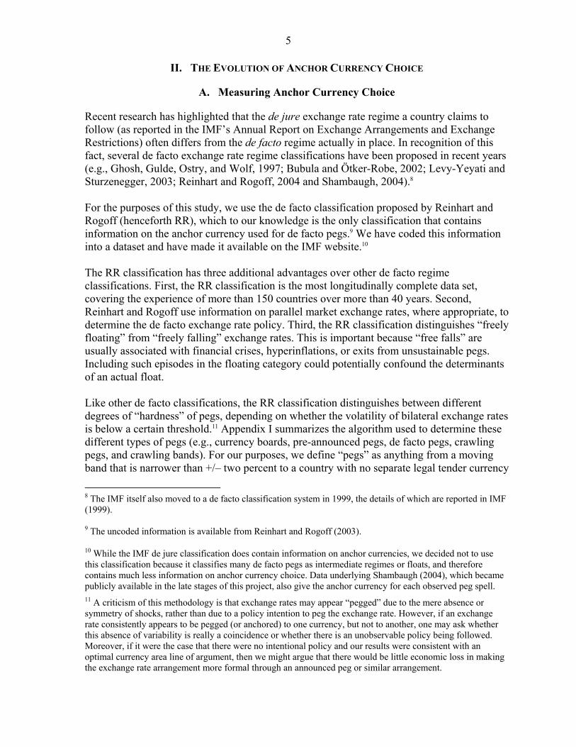
Recent research has highlighted that the de jure exchange rate regime a country claims to follow (as reported in the IMF’s Annual Report on Exchange Arrangements and Exchange Restrictions) often differs from the de facto regime actually in place. In recognition of this fact, several de facto exchange rate regime classifications have been proposed in recent years (e.g., Ghosh, Gulde, Ostry, and Wolf, 1997; Bubula and Ötker-Robe, 2002; Levy-Yeyati and Sturzenegger, 2003; Reinhart and Rogoff, 2004 and Shambaugh, 2004).8 For the purposes of this study, we use the de facto classification proposed by Reinhart and Rogoff (henceforth RR), which to our knowledge is the only classification that contains information on the anchor currency used for de facto pegs.9 We have coded this information into a dataset and have made it available on the IMF website.10 The RR classification has three additional advantages over other de facto regime classifications. First, the RR classification is the most longitudinally complete data set, covering the experience of more than 150 countries over more than 40 years. Second, Reinhart and Rogoff use information on parallel market exchange rates, where appropriate, to determine the de facto exchange rate policy. Third, the RR classification distinguishes “freely floating” from “freely falling” exchange rates. This is important because “free falls” are usually associated with financial crises, hyperinflations, or exits from unsustainable pegs. Including such episodes in the floating category could potentially confound the determinants of an actual float. Like other de facto classifications, the RR classification distinguishes between different degrees of “hardness” of pegs, depending on whether the volatility of bilateral exchange rates is below a certain threshold.11 Appendix I summarizes the algorithm used to determine these different types of pegs (e.g., currency boards, pre-announced pegs, de facto pegs, crawling pegs, and crawling bands). For our purposes, we define “pegs” as anything from a moving band that is narrower than +/– two percent to a country with no separate legal tender currency

8 The IMF itself also moved to a de facto classification system in 1999, the details of which are reported in IMF (1999). 9 The uncoded information is available from Reinhart and Rogoff (2003).

10 While the IMF de jure classification does contain information on anchor currencies, we decided not to use this classification because it classifies many de facto pegs as intermediate regimes or floats, and therefore contains much less information on anchor currency choice. Data underlying Shambaugh (2004), which became publicly available in the late stages of this project, also give the anchor currency for each observed peg spell. 11 A criticism of this methodology is that exchange rates may appear “pegged” due to the mere absence or symmetry of shocks, rather than due to a policy intention to peg the exchange rate. However, if an exchange rate consistently appears to be pegged (or anchored) to one currency, but not to another, one may ask whether this absence of variability is really a coincidence or whether there is an unobservable policy being followed. Moreover, if it were the case that there were no intentional policy and our results were consistent with an optimal currency area line of argument, then we might argue that there would be little economic loss in making the exchange rate arrangement more formal through an announced peg or similar arrangement.

6

(i.e., anything from category 1 through 11 in Table A1 in Appendix I).12 We define “floats” as consisting of either managed floating or freely floating regimes. Following RR, we also include “freely falling regimes” as a separate category distinct from floating and pegging.

Figure 1. All Countries: Anchor Currency Choices, 1950–2001 (Percentage of countries)

0%

20%

40%

60%

80%

100%

1950 1955 1960 1965 1970 1975 1980 1985 1990 1995 2000

year

Perc

ent o

f Tot

al O

bs. Other

EuroFallMarkFrancPoundUSDFloat

B. Stylized Facts on Anchor Currency Choice

In this section, we present some stylized facts on anchor currency choice that emerge from studying the RR dataset discussed above. Perhaps the most interesting stylized fact is that, as Figure 1 shows, virtually all countries that have chosen to peg their exchange rates in some way to another currency have converged over the last fifty years to using either the U.S. dollar or the euro as their anchor currency.13 The “other” category has included at various times the Japanese yen, the Dutch guilder, the Belgian franc, and the Indian rupee, among others. Surprisingly, there has been no significant Japanese yen bloc, as noted before by Camdessus (1995, pp.1–2), who stated that “…the role of the yen is not commensurate with the relative size of the Japanese economy or with Japan’s emergence as the world’s largest creditor country.” One possible reason for this is that Japan had a de facto U.S. dollar anchor from 1949–1977 which simply promoted the use of the U.S. dollar in Asia.14 According to Tavlas and Ozeki (1992), another 12 As part of our robustness checks, we eliminated the countries with a fine classification between 9 and 11 from our pegs. That is, we no longer considered wide crawling bands, de facto crawling bands, and moving bands as pegs. 13 We include only independent countries in these figures. 14 One reason why Japan preferred the U.S. dollar to the British pound was that U.S. economic aid during the reconstruction period and the windfall demands of the Korean war promoted dollar transactions, while the British pound had the disadvantage of nonconvertibility. Thereafter, the dollar stabilized its position as the key currency for Japan, because trade in dollars also increased its share in the Asian region, and trade finance in the New York money market became more important (Iwami, 1994).

7

factor that inhibited the use of the yen as an international currency is that the Tokyo financial market was tightly regulated until the end of the 1980s. Between 1950 and 1972, the U.S. dollar was the most popular anchor currency chosen by developed countries, followed by the British pound sterling and the German mark (Figure 2). Note that, contrary to conventional wisdom, the RR classification suggests that not all countries that were pegging were pegged to the dollar during the Bretton Woods period. There are two reasons for this. First, based on official announcements about the reference currency and policy goals, RR determined that a country like Australia should be classified as having a de facto peg to the pound rather than the dollar, even though the pound itself was pegged to the dollar. Second, by looking at parallel market exchange rates, RR determined that many de jure dollar pegs in Europe during the Bretton Woods period were de facto floating.

Figure 2. Developed Countries: Anchor Currency Choices, 1950–2001 (Percentage of countries)

0%

10%

20%

30%

40%

50%

60%

70%

80%

90%

100%

1950 1955 1960 1965 1970 1975 1980 1985 1990 1995 2000

year

Perc

ent o

f Tot

al O

bs. Other

EuroFallMarkFrancPoundUSDFloat

Following the collapse of Bretton Woods, the anchor currency distribution among developed economies changed considerably and quickly. The U.S. dollar declined significantly in popularity, and the British pound disappeared entirely from the menu of anchor choices. The breakup of Bretton Woods gave rise to an increased number of free and managed floaters, but the majority of developed countries ended up pegging their currency to the German mark. This increased popularity of the German mark was obviously related to the exchange rate mechanism (ERM) leading up to the introduction of the euro. For developing countries (Figure 3), the predominant anchor currencies between 1950 and 1972 were the U.S. dollar, the British pound, and the French franc. Following the collapse of Bretton Woods, de facto pegs declined only gradually. Developing countries followed developed countries in abandoning the British pound sterling as an anchor. However, whereas developed countries replaced the pound with the German mark, developing countries largely switched to using the U.S. dollar as their anchor. A group of former French colonies continued to peg to the French franc. The only (non-transition) developing countries that adopted a German mark anchor were Malta (1978-1998) and Turkey (1998).

8

Figure 3. Developing Countries: Anchor Currency Choices, 1950–2001

(Percentage of countries)

0%

20%

40%

60%

80%

100%

1950 1955 1960 1965 1970 1975 1980 1985 1990 1995 2000

year

Perc

ent o

f Tot

al O

bs. Other

EuroFallMarkFrancPoundUSDFloat

Following the breakup of the Soviet Union in the early 1990s, and the associated price liberalizations and hyperinflations, most transition economies ended up in the “freely falling” category for several years. They then increasingly started pegging their currencies, either tightly or loosely, to the German mark and the U.S. dollar. Figure 4 shows that the choice of anchor currency was curiously divided along regional lines: Central and Eastern European countries chose to anchor to the German mark (later the euro), while most former Soviet Union republics chose the U.S. dollar as their anchor currency (with the exception of Estonia, which adopted a currency board arrangement with the German mark as anchor; and Latvia, which chose the SDR). By 2001, seven transition countries were anchored to the euro, eight countries (all CIS) were anchored to the U.S. dollar, one country (Latvia) was pegged to the SDR, five were freely floating, and two were freely falling.

Figure 4. Transition Countries: Anchor Currency Choices, 1990–2001 (Percentage of countries)

0%

10%

20%

30%

40%

50%

60%

70%

80%

90%

100%

1990 1995 2000

year

Perc

ent o

f Tot

al O

bs.

OtherEuroFallMarkUSDFloat

9

C. Why Countries Peg the Way They Peg: A Brief Survey of Recent Experience

Some examples from recent anchor choices may be illustrative in highlighting that trade network externalities and other optimal currency area considerations matter for anchor choice. One example is Estonia’s decision to anchor to the German mark and later the euro. The rationale for this decision was described as follows: “The tightening or loosening of the monetary environment by the ECB does not contradict the trends of domestic monetary conditions, because close to 70 percent of Estonia's foreign trade is with the EU. This means that the possibility of being in a fundamentally different phase of the economic cycle than the EU is not likely to occur…” (Kraft, 1999, p.1). Another example is constituted by the countries associated with the East Caribbean Currency Authority, all of which switched from a sterling peg to a dollar anchor in the 1970s. The factors that motivated this switch included (1) increased trade relations with the United States; (2) increased trade with countries in the Caribbean free trade area CARICOM, many of which also pegged to the U.S. dollar; and (3) declining trade with the United Kingdom (Worrell, Marshall and Smith, 2000; East Caribbean Economic and Financial Review, 1976). In the West African Monetary Zone (WAMZ), the anchor choice recently discussed has been the U.S. dollar, given that all WAMZ countries quote their exchange rates in terms of the dollar, and most of their external reserves are held in dollars (WAMI News, 2002, p. 13). However, since the WAMZ intends to eventually merge with the CFA franc zone (which is now pegged to the euro), there is discussion about what the common anchor will be. Special relationships derived from colonial experience between France and the countries in the CFA franc zone have thus far sustained this anchor, but it is unclear whether the euro peg would be sustained in the planned larger monetary union in the Economic Community Of West African States (ECOWAS) that would merge former French and British colonies. Dilution of these political ties to France is a concern. One possibility being discussed is to peg this larger monetary union’s currency to the SDR as a compromise (WAMI News, 2003). Elsewhere in Africa, the Southern African Development Community (SADC) aims to establish a common currency by 2018, and the African Union has considered the idea of adopting a single continental currency. Yehoue (2006) argues that this currency should be pegged to the euro because of more intense trade relations with the euro area.15 In the Middle East, the six members of the Gulf Cooperation Council (Bahrain, Kuwait, Oman, Qatar, Saudi Arabia, and the United Arab Emirates) are planning to establish a common currency by 2010 (Fasano and Schaechter, 2003). They originally planned to peg this currency to the U.S. dollar, since this would help to reduce uncertainty about oil export income, given that oil exports are priced in dollars. However, in preliminary discussions, the weakening dollar and increased integration with Europe via new trade agreements have been

15 For more on African monetary unions, see Masson and Pattillo (2005) and Yehoue (2004, 2006).

10

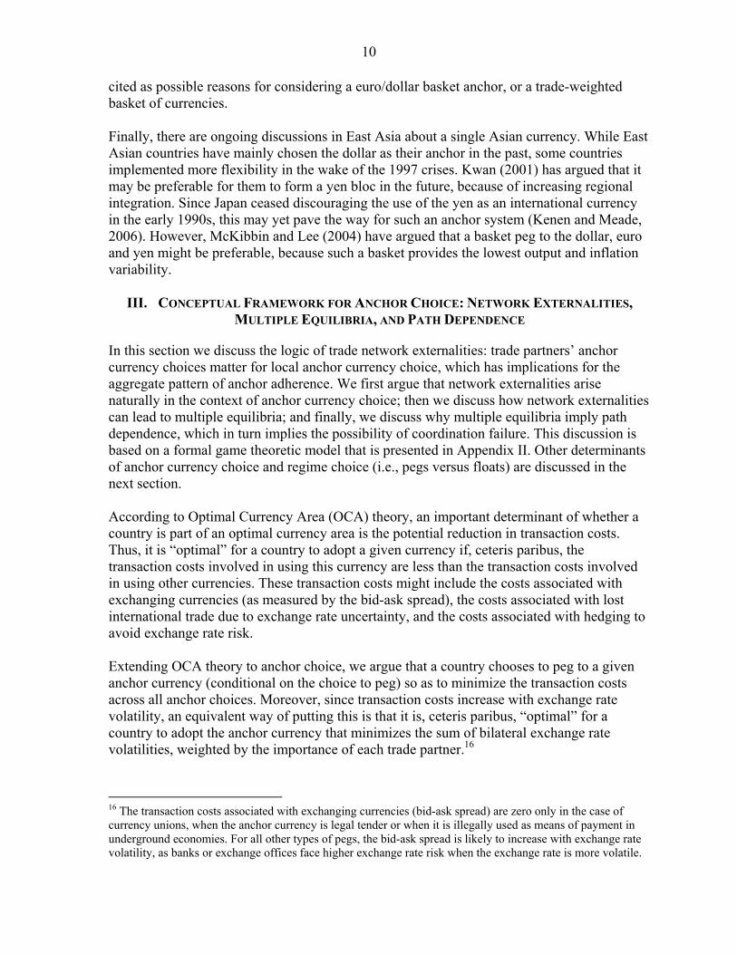
cited as possible reasons for considering a euro/dollar basket anchor, or a trade-weighted basket of currencies. Finally, there are ongoing discussions in East Asia about a single Asian currency. While East Asian countries have mainly chosen the dollar as their anchor in the past, some countries implemented more flexibility in the wake of the 1997 crises. Kwan (2001) has argued that it may be preferable for them to form a yen bloc in the future, because of increasing regional integration. Since Japan ceased discouraging the use of the yen as an international currency in the early 1990s, this may yet pave the way for such an anchor system (Kenen and Meade, 2006). However, McKibbin and Lee (2004) have argued that a basket peg to the dollar, euro and yen might be preferable, because such a basket provides the lowest output and inflation variability.

III. CONCEPTUAL FRAMEWORK FOR ANCHOR CHOICE: NETWORK EXTERNALITIES, MULTIPLE EQUILIBRIA, AND PATH DEPENDENCE

In this section we discuss the logic of trade network externalities: trade partners’ anchor currency choices matter for local anchor currency choice, which has implications for the aggregate pattern of anchor adherence. We first argue that network externalities arise naturally in the context of anchor currency choice; then we discuss how network externalities can lead to multiple equilibria; and finally, we discuss why multiple equilibria imply path dependence, which in turn implies the possibility of coordination failure. This discussion is based on a formal game theoretic model that is presented in Appendix II. Other determinants of anchor currency choice and regime choice (i.e., pegs versus floats) are discussed in the next section.

According to Optimal Currency Area (OCA) theory, an important determinant of whether a country is part of an optimal currency area is the potential reduction in transaction costs. Thus, it is “optimal” for a country to adopt a given currency if, ceteris paribus, the transaction costs involved in using this currency are less than the transaction costs involved in using other currencies. These transaction costs might include the costs associated with exchanging currencies (as measured by the bid-ask spread), the costs associated with lost international trade due to exchange rate uncertainty, and the costs associated with hedging to avoid exchange rate risk. Extending OCA theory to anchor choice, we argue that a country chooses to peg to a given anchor currency (conditional on the choice to peg) so as to minimize the transaction costs across all anchor choices. Moreover, since transaction costs increase with exchange rate volatility, an equivalent way of putting this is that it is, ceteris paribus, “optimal” for a country to adopt the anchor currency that minimizes the sum of bilateral exchange rate volatilities, weighted by the importance of each trade partner.16

16 The transaction costs associated with exchanging currencies (bid-ask spread) are zero only in the case of currency unions, when the anchor currency is legal tender or when it is illegally used as means of payment in underground economies. For all other types of pegs, the bid-ask spread is likely to increase with exchange rate volatility, as banks or exchange offices face higher exchange rate risk when the exchange rate is more volatile.

11

Since effective bilateral exchange rate volatility depends on the anchor currency choices of a country’s trade partners, one country’s optimal anchor choice is naturally a function of other countries’ anchor choices. In other words, the transaction cost saving property of pegged exchange rate regimes gives rise to network externalities (or strategic complementarities) in anchor choice. The notion of network externalities in currency choice is not entirely new. For example, OCA theory itself states that the transaction cost savings associated with using a particular currency increase with the share of transactions carried out in that currency. The same is highlighted in a sizeable recent literature including Kiyotaki and Wright (1989), Dowd and Greenaway (1993), Flandreau (1996), Eichengreen and Flandreau (1998), and Meissner (2005). All of these contain discussion on how these types of externalities matter for monetary regimes. Similarly, in the related literature on international currency use, the existence of “economies of scale” has been emphasized (e.g., Krugman, 1984), and Tavlas and Ozeki (1992) argued that a condition that reinforces international currency use is “the amount of trade invoiced in a currency.” Network externalities typically imply multiple equilibria. While this is shown formally in a model in Appendix II, the intuition behind this model can be easily understood. First, assume for simplicity that your only goal is to minimize transaction costs. This implies that, when all of your trade partners are using the U.S. dollar as anchor, your best response is to coordinate and choose the dollar as well. However, if for some reason all of your trade partners had chosen the euro as anchor, then your best response would be to choose the euro as well. This implies that there exist as many equilibria as there are anchors. Now suppose that, in addition to caring about transaction costs, countries also have additional, idiosyncratic reasons for preferring a particular anchor. In this sense, anchors are very much like industrial or technological standards, in that what makes them useful is a combination of their inherent qualities and the extent to which others are using them. If the externalities are more important than the inherent qualities, that is, if the benefits from coordination are sufficiently large, network externalities tend to give rise to multiple equilibria. However, if the inherent qualities of are significantly better, or if users have particular idiosyncratic characteristics that make certain anchors or standards significantly better for them, multiple equilibria may not arise, as shown in Appendix II. Finally, the existence of network externalities in anchor currency choice implies the possibility of path dependence and coordination failure (e.g., Arthur, 1989). To see this, assume for simplicity that the world consists of only two countries, i and j, and each country has a choice between two anchor currencies: the U.S. dollar ($) and the euro (€), the payoffs associated with which are given in Tables 1 and 2.

Table 1. Initial Payoff Matrix

Aj = $ Aj = €

Ai = $ 3,1 2,0.5

Ai = € 0,0 1,1.5

12

Table 2. Subsequent Payoff Matrix

Aj = $ Aj = €

Ai = $ 1,1 0,0.5

Ai = € 0.5,0 1.5,1.5

The payoff matrix in Table 1 assumes that choosing a dollar anchor has payoffs for country i that are independent of the trade partner’s anchor choice (e.g., because country i exports commodities that are priced in dollars or has significant liabilities that are denominated in dollars), and these payoffs are large enough so that country i will always prefer to peg to the dollar. That is, pegging to the dollar is a dominant strategy for country i. Country j, instead, enjoys some euro-specific payoffs, but these payoffs are not large enough to offset dollar bloc network externalities. Then, according to the payoffs in Table 1, the unique Nash equilibrium is for both countries to peg to the dollar, even though country j would be better off if both pegged to the euro. In the latter case, j would get the idiosyncratic benefits plus similar reductions in transaction costs via coordination. Now suppose that, starting out from the dollar-dollar equilibrium, the dollar-specific payoffs to country i disappear (for example, because country i exports oil and oil is no longer priced in dollars), while both countries now enjoy some euro-specific payoffs, as in Table 2. Now there are two Nash equilibria again, and both countries would be better off to switch to the Nash equilibrium in which both are pegging to the euro. However, in the absence of any communication or coordination between the two countries, country i will continue to peg to the dollar because country j does so, and j continues to do so because i does so. Thus, the choice of the dollar is path dependent. In this example, the path dependence actually implies a coordination failure in the sense that both countries would be better off if they simultaneously decided to switch to pegging to the euro, or perhaps decided to create a local monetary arrangement.17 While re-coordinating in a two-country world would be relatively simple, the complexity of negotiating another arrangement when more countries are involved could delay or even deter the emergence of the socially optimal arrangement—the time it took to establish EMU is a case in point. An actual example of a possible coordination failure is the popularity of U.S. dollar anchors in many former Soviet Union countries, most of which trade more with the euro area than with the United States. These countries might benefit from a coordinated switch from a dollar to a euro anchor, but this may be hard to achieve. However, once a few important countries let go of the dollar anchor (e.g., because the dollar continues to depreciate relative to the

17 Ogawa and Ito (2000) present a model that displays such possibilities. Yehoue (2004) studies currency union formation in a dynamic setup and demonstrates trade flows to be an important determinant.

13

euro), their trade partners could do the same and, hence, the dollar equilibrium could rapidly unravel.18

IV. EMPIRICAL METHODOLOGY

In our empirical approach, we use a multinomial logit setup to control for trade flows and other determinants of anchor choice. The categories in the multinomial logit likelihood function that we use are: peg to the U.S. dollar, peg to the French franc, peg to the German mark, float, and freely fall.19 We also control for the choice to peg in the first place (to any anchor), by simultaneously modeling the choice of exchange rate regime and the choice of anchor. We use the country-year as the observational unit.20 The payoffs to country i in year t from a peg to any particular anchor currency A (where A is an element of the set of all possible anchors) can thus be written as: where βA measures the strength of network externalities, tijt is the share of GDP of country i’s trade with country j in year t, is the trade-weighted number of trade partners that peg to anchor A in year t, and the residual A

ite measures a random unobservable component to the choice of anchor A.21 18 A similar event took place with the dissolution in the 1970s of the Sterling bloc, the reasons for which are discussed in more detail in Section VI. A rather quick and coordinated switch from a sterling anchor to a dollar anchor took place in the mid-1970s by countries in the East Caribbean Currency Authority. The spark that ignited the switch was the depreciation of sterling against the U.S. dollar (East Caribbean Economic and Financial Review, 1976). These countries were able to coordinate a quick switch because good infrastructure existed for communication between the countries. However, in more dispersed and politically fragmented groups of countries, one would expect a longer delay at a given level of benefits.

19 While anchor regime data prior to 1972 include other anchors, the complete set of control variables only allowed us to use these three anchors in our tests. For example, it was infeasible, given our control variables, to include anchors like the yen, the Rand or the Australian dollar, which had very few actual adherents. We were able to include the British pound in years prior to 1980 by eliminating certain control variables, but decided against presenting these results because the costs (having to eliminate important regressors) exceeded the payoffs (one extra anchor, but similar results on network externalities and other anchor variables). 20 Eichengreen and Bayoumi (1999) look at de facto pegs in a slightly different way. They regress bilateral exchange rate volatility on the level of bilateral trade, the synchronicity of output shocks, and several other variables to control for the choice of whether to peg or not. This approach, unlike ours, is unable to explain why two small countries that both peg to the dollar, and that have little bilateral trade, but lots of trade with the United States, would have such low bilateral exchange rate volatility. These countries would be extreme outliers to the extent that only bilateral trade flows matter in their final specification. In addition, Eichengreen and Bayoumi’s (1999) approach looks at the choice as a bilateral option with a simple linear relationship, while we prefer to think of the choice between blocs as a possibly highly nonlinear relationship. Finally, our sample is much broader than theirs. 21 We divide trade by GDP, so we can interpret this roughly as the empirical probability that a transaction made by a local resident will take place with the anchor country or a country pegged to the anchor.

∑ ∑ ∑∑ ++++⎥⎦

⎤⎢⎣

⎡==

k l m

Aittm

Amitl

Peglitk

Ak

jjtijt

AAit ezyxAAItU ββββ )(

( )ApAAIt jtj

jtijt ≡=∑ )(

(1)

14

To estimate country-specific preferences, the vector itkx contains the K observed characteristics (k = [1,…,K]) of country i that affect the anchor choice A. These include the amount of liabilities denominated in currency A, the symmetry of output shocks, and a country’s past experience with an anchor. The vector itly contains the L country-specific characteristics (l = [1,…,L]) that affect the choice of whether to peg to any anchor (e.g., economic size, openness, reserve cover, and financial development). The vector tmz contains the M anchor-specific characteristics (m = [1,…,M]) that affect anchor choice (e.g., the level and variability of inflation in the anchor-currency issuing country). The elements of itkx , itly , and itmz are described in detail in the next section. Note that the coefficients on variables that affect anchor choice are allowed to vary over regimes and anchor choices, while the coefficients on y, the variables that determine the value of pegging, are constrained to be the same over all anchor choices because all anchors are pegs. We normalize the payoff from floating to 0 and assume that the payoff from freely falling is given by

Fall Fall Fallit k itk it

kU y eβ= +∑ .

We constrain the coefficients for a number of variables to equal zero, based on a priori theoretical reasoning and the limits of the data. The vector of country characteristics that enters the “choice” to fall is the same as that for the choice to peg, but the coefficients are allowed to differ. We also constrain the parameters associated with anchor choice (i.e., the trade links variable and the vector of characteristics x) to be zero for the freely falling category. Finally, some other coefficients are constrained to be zero for various anchors, due to data constraints. For example, no Latin American country had a mark peg so this makes it impossible to estimate a coefficient on a regional dummy for Latin America for the mark anchor choice. Importantly, we constrain the coefficients on the variables that determine the value of pegging to be the same across all anchor choices. The relative probability of any two anchors in this case does not depend on factors affecting the decision to float or peg. An alternative specification that we considered (but do not report) is the nested logit model. In such a model, a country would be assumed to first choose whether to peg, float or freely fall, and only then (after having decided to peg) to choose amongst a set of anchor currencies. The natural benefit of using nested logit is that, over certain groups of choices, one can relax the Independence of Irrelevant Alternatives (IIA) assumption that is inherent in the multinomial logit model. In intuitive terms, an unconstrained multinomial logit makes it such that if an equally attractive anchor to the dollar, say, appears on the scene, then the predicted sample frequency of all types of pegs relative to floats and free falls would increase. This is clearly not desirable and seems quite unrealistic. The set of anchors is relatively fixed over the sample period 1980-1998 (and even in the long run) so the thought experiment is not very applicable. Aside from the list of anchors we include, there are very few other viable choices for anchors, as Figure 1 shows.

(2)

15

We tried several nested logit specifications, but did not find any evidence of unobservable common traits amongst our anchor choices that would show up if the multinomial framework were invalid. We also tested the IIA assumption by excluding each anchor choice and re-estimating the multinomial logit models specified above, but we did not find much evidence against IIA.22 Below, we also report specifications where we restrict attention to anchor choice only.

V. EMPIRICAL DETERMINANTS OF ANCHOR AND REGIME CHOICE

This section describes the control variables included in our regressions, and our rationale for including them. We split the variables into three groups: (A) country-specific determinants of anchor currency choice; (B) country-specific determinants of regime choice (i.e., peg, float, fall); and (C) anchor-specific determinants of anchor currency choice. Group A variables include trade links with a particular bloc, the symmetry of output shocks, the currency denomination of debt, the commodity composition of exports, and shared legal, colonial, or political histories, as proxied by regional indicators. Group B variables include economic size, openness to international trade and capital flows, the nature of macroeconomic shocks, financial development, the need for credibility, and past regime choice. Finally, the key variables for group C are the historical (10-year average) level of inflation in the country issuing the anchor currency, and the standard deviation of the annual average inflation rate in the anchor-issuing country during the previous 10 years.

A. Country-Specific Determinants of Anchor Currency Choice

The three country-specific determinants of anchor currency choice we focus on are (a) trade network externalities; (b) output co-movement, and (c) the currency denomination of liabilities. The importance of output co-movement is derived from OCA theory, which suggests that there are costs to pegging to a particular anchor currency when there are large asymmetries in output shocks, or low co-movement of output. The larger the asymmetries in the shocks between one country and a particular currency bloc, the more costly it is for this country to choose the same anchor as the currency bloc. We operationalize these asymmetries by including as an anchor choice determinant the standard deviation of the difference of log growth rates of real output over the previous fifteen years, where the difference in growth rates is taken between country i and the country that supplies the anchor currency. OCA theory was born in an era when international capital movements were relatively limited. But in the recent past, with increased capital account liberalization and development prospects, international capital flows denominated in foreign currencies have been very important for a large group of countries, thus making the currency denomination of capital 22 For example, we left out the franc anchor option and the variables associated with this anchor choice, and reestimated the multinomial logit including only the dollar, mark, fall and float options. We then compared the estimated coefficients on the choices affecting a dollar anchor in this specification to the full specification. Many of our Hausman-type tests did not meet the necessary asymptotic criteria, but the coefficient magnitudes did not seem to change too much.

16

flows an important variable. We hypothesize, therefore, that, conditional on the choice to peg, countries choose the anchor currency for those pegs in order to minimize the exchange rate volatility with the currencies in which their liabilities are denominated. That is, the more U.S. dollar denominated liabilities a country has, the more likely this country is to adopt the dollar as an anchor for its peg. As a proxy for these liabilities, we use data made available by the Bank for International Settlements on the level of total gross outstanding claims (loans, securities and other liabilities) to all sectors issued abroad and denominated in the anchor currencies. We convert all values into U.S. dollars.23 As with trade, we normalize these liabilities by nominal GDP.

B. Country-Specific Determinants of Regime Choice: Pegs vs. Floats

Because we simultaneously estimate the choice of exchange rate regime and the choice of anchor, we need to control for factors that determine the choice whether or not to peg in the first place (to any anchor). To do this, we consider a large set of possible determinants obtained from both the theoretical and the empirical literature on exchange rate regime choice. First, we control for trade openness, or the size of international trade relative to GDP. Theoretically, the effect of openness on regime choice could go either way. On the one hand, higher trade openness implies a higher payoff (in terms of saving on transaction costs) from pegging an exchange rate to any possible anchor, suggesting that more open countries may be more likely to adopt a pegged exchange rate regime. On the other hand, countries that trade a lot are more exposed to terms of trade shocks and could therefore benefit more from flexibility in the nominal exchange rate, leading to the opposite conclusion, that more open countries may in fact be more likely to adopt a flexible exchange rate regime. Our data come from the IMF International Financial Statistics (IFS) database. Trade openness is measured as total imports and exports divided by PPP adjusted GDP, where the numerator and denominator are measured in real terms. Second, we control for capital account openness. Its effect on regime choice is also theoretically ambiguous. On the one hand, countries that borrow abroad may have strong incentives to peg their exchange rate. When there are no hedging mechanisms to avoid exchange rate uncertainty, or when the use of such hedging mechanisms is expensive, an exchange rate peg can ensure that the volatility of returns is not affected (too much) by exchange rate volatility. On the other hand, large capital flows and a pegged exchange rate are not compatible with an independent monetary policy, according to the Trilemma argument (see, for example, Obstfeld and Taylor, 1998). Hence, countries exposed to large capital flows may be more likely to opt for a float in order to avoid loss of independent monetary policy. We measure capital account openness as in Juhn and Mauro (2002). This is the total of gross capital inflows and outflows divided by nominal GDP. The data come from the IFS.

23 The data were graciously provided to us by Ugo Panniza. Some indication of the construction of the data and the sources is given at http://www1.oecd.org/dac/debt/. We also exclude some of the countries with the highest debt to GDP values as these appeared to be extreme outliers.

17

Third, we control for reserves. Countries holding large amounts of reserves can more easily maintain the credibility of a peg and so may be more likely, all else equal, to choose a pegged exchange rate. In a simple first generation currency crisis model (e.g., Krugman, 1979), a government running an excessively expansionary policy runs out of reserves over time. This precipitates the speculative action that dooms a peg. The likelihood of seeing a peg in any given year, then, is a function of international reserves. We normalize reserves by M2. All data come from the IFS. Fourth, we control for financial development. The effect of this is again theoretically ambiguous. On the one hand, financially developed countries may be more successful at adopting and maintaining pegs. Prudent regulation of the banking system and financial markets may allow for a deep financial system to emerge and more sustainable outcomes, rather than booms, busts, and the eventual currency crisis due to oversight, recklessness and cronyism. On the other hand, as argued in Levy-Yeyati, Sturzenegger and Reggio (2003), a more developed financial system could be synonymous with greater exposure to international capital flows. For countries wishing to maintain autonomous monetary policy, this would mitigate against the choice of a peg. To measure financial development, we use the proportion of M2 in the total monetary stock. All monetary data come from the IFS. A fifth control is inflation history. The argument here is that countries with a history of high inflation may be more interested in trying to “import” monetary policy credibility by pegging the exchange rate to the currency of a country with a reputable monetary authority, or by foregoing control over monetary policy altogether. In part for this reason, the recent past has seen the implementation of new currency boards in Argentina, Bosnia and Herzegovina, Bulgaria, Djibouti, Estonia, and Lithuania. Moreover, various types of more flexible pegs are often regarded as mechanisms to focus inflationary expectations and hence to control actual inflation. We measure the potential need to import policy credibility with an indicator variable that takes the value one when a country experienced a bout of “high inflation” between the current year and 1950. We define a country to have had “high inflation” if the country had entered the freely falling category, as defined in the Reinhart and Rogoff data. We allow the coefficient of this factor to differ by anchor to see if particular anchor currencies have differential benefits in this regard. Sixth, according to standard open-economy macroeconomic theory embodied in the Mundell-Fleming-Dornbusch type of models, countries with large real shocks relative to nominal shocks might prefer to use the nominal exchange rate as a shock absorber, and therefore might be less likely to peg. Conversely, in countries where nominal shocks are more important, a peg or quasi-peg can eliminate or reduce these shocks by forcing the money supply to adjust in the appropriate direction. We measure real shocks with the volatility of the previous five-year’s investment to GDP ratio. Exposure to nominal shocks is measured by the volatility of the previous five-years’ velocity of the money supply. Data on the money supply and real output come from the IFS. Seventh, we include the logarithm of real GDP and the logarithm of population. Larger countries may be less likely to focus on the trade-enhancing benefits of a peg since they are less reliant on international trade. Moreover, richer countries often have more policy credibility and hence are less likely peg. GDP and population data come from the World Bank’s World Development Indicators.

18

Finally, we include the lagged regime choice as a control, to capture the notion that countries are not likely to actively engage in a decision making process about their regime year-in-year-out. If we were to use a standard multinomial logit model with no control for past outcomes on a panel data set, we would be implicitly assuming that the choice was taken independently in each and every year regardless of previous experience.24 There would also likely be serial correlation in regime choice, making inference problematic. A more realistic assumption then might be that countries come to a point when a decision needs to be made and that decision persists until events change radically—for example, in case of a speculative attack, a major political event or a major economic shock. To capture this idea of persistence, we include the lagged values of regime choice in Table 3, and the lagged values of anchor choice in Table 4.25

C. Anchor-Specific Determinants of Anchor Currency Choice

To reflect the hypothesis that “stable” currencies are more likely to be chosen as anchors, we control for the average level and variability of inflation in the anchor country over the previous ten years. Goodhart (1989) and Kouri and Macedo (1978) emphasize the importance of comparative price stability for the choice of an international currency. We were unable to find any statistical relationship between the level of inflation or its standard deviation and anchor choice. We do not report any results that include these variables. The most likely reason for this result is that the anchors in our dataset did not differ enough in terms of their inflation properties so as to be discernible in the estimation. While it is hard to believe that a viable anchor would have a bad inflationary track record, testing this in the context of our econometric model is difficult because we must focus on choices that have actually been taken. For example, it would have been impossible to test whether inflation in Mexico has been a factor limiting the choice of peso anchors, because there are no peso anchors in our dataset. Similarly, it would be difficult to argue that high inflation in

24 Our dataset combines observations that have transitions into pegs, floats or falls and observations that have continuing pegs, floats and falls. With the exception of a few types of changes, transitions from different regimes are relatively rare since the RR data are smoothed and allow for parity changes. This is one reason to pool all the data and simply use lagged indicator variables to allow for state dependent transition probabilities. Nevertheless, one might want to estimate a full conditional transition model. One might do this under the assumption that different variables or changes and levels of variables affect regime choice in any given year differently. In addition to a pooled multinomial approach, we thus tried to run an unrestricted transition model (see Beck, Epstein, Jackman and O’Halloran, 2002). We ran two multinomial logits. One had only observations that stayed in the same regime as the previous year and one had only observations that moved into their current regimes from a different regime. The assumptions about duration dependence and state independence are strong in such a model, but practically speaking, the data do not allow for much more. In any case, we find that our baseline model, itself a restricted transition model, is for all intents and purposes the same as running the unrestricted transition model. In other words, most of the identification of our coefficients is coming from between-country differences in variables as they relate to similar long-run regime choices. 25 In addition, we included in some specifications a set of time indicators which can, under certain assumptions, allow for duration dependence or serial correlation in regime choice (see Maddala, 1987 or Beck, Katz and Tucker, 1997 and Bernhard and Leblang, 1999). We eliminated some of the controls for lagged regimes, since in practice there is no data for such observations. For example, no country moved from a mark anchor to a dollar anchor in our sample. A look at the information contained in the sample transition probability matrix will show other constraints the data impose.

19

Mexico raised the probability of pegging to the dollar for sample countries, since this may as well have been due to high inflation in Iceland or any other country that experienced high inflation at that time.26

VI. RESULTS

The output from our maximum likelihood estimates are reported in Tables 3 through 6. Table 3 provides results for a sample ranging between 1990 and 1998, which are the years for which detailed data on currency denomination of liabilities is available. In our baseline specification of Table 3, we study the limited period 1990-1998 because our debt data begin only in 1990, while other series do not stretch into the 21st century. Table 4 covers a longer period, 1980 to 1998, since we leave out the currency denomination of debt variable here. Other sensitivity checks extend the sample further backward and forward without changing the qualitative results on the determinants of anchor choice. Table 5 restricts the choice set to only the anchors (dollar, franc and mark). Table 6 restricts the choice set to the anchors, uses cross-sectional data for 1998 and controls for the possible endogeneity of trade relations with the anchor blocs. Throughout, we report the estimated coefficients that are related to the odds-ratios of one choice versus another choice.

A. Determinants of Anchor Currency Choice

Tables 3 and 4 demonstrate findings consistent with OCA theory and network externalities. As predicted, trade network externalities seem to matter for anchor currency choice. This is exhibited by the positive signs on our coefficients on within-bloc trade for anchor choice, reported in Tables 3 and 4. Out of the six estimated coefficients, all are positive and four are statistically significant. Trade relations with the mark bloc are always statistically significant, while the dollar trade flows become insignificant in Table 4 and the franc trade flows are insignificant in Table 3. Nevertheless, they always have the correct sign. In the next section, we provide some way to gauge how important these trade variables might have been for determining the pattern of anchor choice we have seen in the past. The estimated coefficients on the variables associated with symmetry of shocks give some additional support for an “optimal anchor currency area” theory. For dollar and mark anchors, an increased co-movement of nominal output is associated with an increased propensity to adopt that particular anchor. This variable is never statistically significant for the dollar, but it is always statistically significant for the mark. The coefficient on the franc anchor is opposite to what we would expect and to what we see for the other anchors.

26 For the same reason, it is difficult to test for other variables that could be anchor-specific determinants of anchor currency choice. Tavlas and Ozeki (1992 p. 3) argue that, for a country’s currency to become used internationally (for trade to be financed in its currency), this country should possess financial markets that are broad, deep, and substantially free of controls. For example, the dominance of sterling in international trade during the late nineteenth century reflected in part the fact that London was an important financial center. But these variables find the same problems in the data as the control for inflation in the anchor countries.

20

Tabl

e 3.

Det

erm

inan

ts o

f Anc

hor a

nd E

xcha

nge

Rat

e R

egim

e C

hoic

e, 1

990–

1998

21

Tabl

e 4.

Det

erm

inan

ts o

f Anc

hor a

nd E

xcha

nge

Rat

e R

egim

e C

hoic

e, 1

980–

1998

22

The results also suggest that having pegged to a particular anchor in the previous period increases the probability of choosing that anchor again. This is shown in Table 4, where we allow the coefficient on past experience to vary by anchor currency, yielding different coefficients for each feasible state in year t-1. This enables us to see whether having had, for instance, a mark or a dollar anchor in the previous year had a different impact on the propensity to adopt a mark anchor in the current year.27 The results suggest that the coefficient on a lagged dollar anchor in the choice of a dollar anchor was not much different from the coefficient on a lagged mark anchor in the mark choice. However, there are relatively few observations other than this type in the data, which is to say that most dollar anchors are preceded by either dollar anchors or floats in the previous year. No franc anchors in the sample were preceded by other anchors in the previous year. As a result of all this, there is only a limited subset of the possible previous year regime coefficients that are feasibly estimated.

B. How Strong Are Network Externalities?

In order to get a sense of the strength of network externalities, and therefore the likelihood of coordination failure, we measured how strongly trade links and other countries’ choices affect the geography and incidence of particular anchor currencies. Our main finding here is that within-bloc trade is crucial. To show this, we ran the following counterfactual for each type of anchor: We first supposed that, for each country, trade with a given bloc was X percent of actual trade (relative to GDP) with that bloc in each year (where X could take the values 100, 50, and 0). Then we simply substituted this new counterfactual trade level for actual trade and then predicted regime choice.28 One plausible counterfactual would be one which allows us to gauge what might have happened to the other blocs if we apportioned this “lost” trade to trade with these other blocs. Our first finding is that, when half of all trade with the dollar bloc dries up, the dollar bloc also shrinks significantly. Figure 5 plots actual dollar anchors, and predicted dollar anchors for trade at the 100 percent (actual), 50 percent and 0 percent levels when the lost trade is apportioned to the mark bloc. The size of the dollar bloc is almost half the size of the actual bloc when trade with that bloc is completely reduced. In Figure 6, we show what happens to the mark bloc. We present results where we simply add the equivalent of 0, 50, or 100 percent of all trade (relative to GDP) with countries on a dollar bloc to trade with the mark bloc (again, relative to GDP). 27 It was infeasible to allow for this in the baseline specification reported in Table 1 because the particular combinations of variables generate collinearity and extremely good predictions of certain pegs, thus automatically dropping some variable in the maximization process. 28 The highest probability out of the five predicted probabilities determines which type of anchor/regime a country is predicted to have.

23

Figure 5. Actual and Predicted Number of Dollar Anchors, Given x Percent of Actual Trade with the Dollar Bloc, 1990–1998

0

5

10

15

20

25

30

35

40

45

50

1990 1991 1992 1993 1994 1995 1996 1997 1998

Year

Num

ber Actual

50 percent100 percent0 percent

Note: A country is classified as being on a given regime if the predicted probability amongst all regimes is maximal. A score of 50 percent means that trade with the dollar bloc has decreased by 50 percent. Also see text.

Figure 6. Actual and Predicted Number of German Mark Anchors, Given x Percent Decrease of Trade with the Dollar Bloc, 1990–1998

0

5

10

15

20

25

30

35

40

1990 1991 1992 1993 1994 1995 1996 1997 1998

Year

Num

ber Actual

50 percent100 percent0 percent

Note: A country is classified as being on a given regime if the predicted probability amongst all regimes is maximal. A score of 50 percent means that trade with the dollar bloc has decreased by 50 percent, and this value of trade has become trade with the mark bloc. Also see text. A final result based on this exercise is that regime choice is nonlinear in trade flows, in that a relatively small amount of regime change can have large effects on the geography of the international monetary system at certain levels. This is suggested by the finding that the percentage reduction in the number of countries pegging to the dollar is slightly larger when moving from 50 to 0 percent of actual trade than when moving from 100 to 50 percent of actual trade. It appears that, as the bloc diminishes in size, the marginal loss in dollar adherents becomes larger—that is, a snowball effect occurs. This could be due to the logit function itself, and therefore deserves further investigation.

24

C. Other Determinants of Anchor Choice

We find some evidence that regional preferences and the currency denomination of exports matter for anchor choice. This is shown in Tables 3 through 6, where regional controls are included as proxies for political and historical affinities, while the commodity composition of exports is included as a proxy for the currency denomination of exports (since commodities are typically priced in dollars).

Regarding regional preferences, we find that Eastern European states have a preference for mark anchors, while countries in Sub-Saharan Africa and the Middle East are more likely to peg to the franc. Many regions simply have no history with particular anchors. Such is the case with the franc and mark in East Asia, and with the mark in Sub-Saharan Africa. One interpretation of these findings is that older colonial and quasi-colonial or modern political influences are exerting control and serving to focus anchor strategies in various countries.

Regarding the commodity composition of exports, we find little evidence that petroleum exporters, who nearly always denominate their exports in dollars, are more likely to peg to the dollar. However, we do find evidence in Table 3 that primary commodity exporters (excluding oil) are in fact more likely to peg to the dollar.

D. Determinants of Regime Choice: Pegs vs. Floats

The results reported in Table 3 and Table 4 are fairly supportive of the traditional economic factors that have been mentioned as determinants of regime choice, but it is hard to obtain significant and robust effects. This is consistent with Juhn and Mauro’s (2002) finding that there are no robust empirical regularities in how countries choose their exchange rate regimes. Larger economies seem much less likely to peg their exchange rates. Countries with greater volatility of real shocks are also less likely to peg. Results on monetary shocks are ambiguous. In Table 3, the coefficient is opposite to the standard prediction, because larger volatility of the money supply is associated with a lower likelihood of a peg. In Table 4, this variable is not statistically significant. In Table 3, trade openness is negatively associated with pegging (but statistically insignificant), but in Table 4 it is positively associated with pegging and statistically significant. Other variables that are not statistically significant include financial development, the ratio of reserves to total money, and capital account openness. However, it is interesting to note that the latter variable has a negative coefficient on the likelihood of seeing a free fall. This is possibly because the countries that have seen the largest gross capital flows in the past two decades have been the economically developed countries, which are more likely to float. There is strong evidence that countries use pegs (at least U.S. dollar anchors and German mark anchors) to regain credibility or stabilize inflation. The coefficients on the past hyperinflations variable for dollar and mark anchors are positive and statistically significant in Table 3. In Table 4, past hyperinflations are not significant determinants of pegging to the dollar or mark. Perhaps this is because many transition countries that ended up pegging in the

25

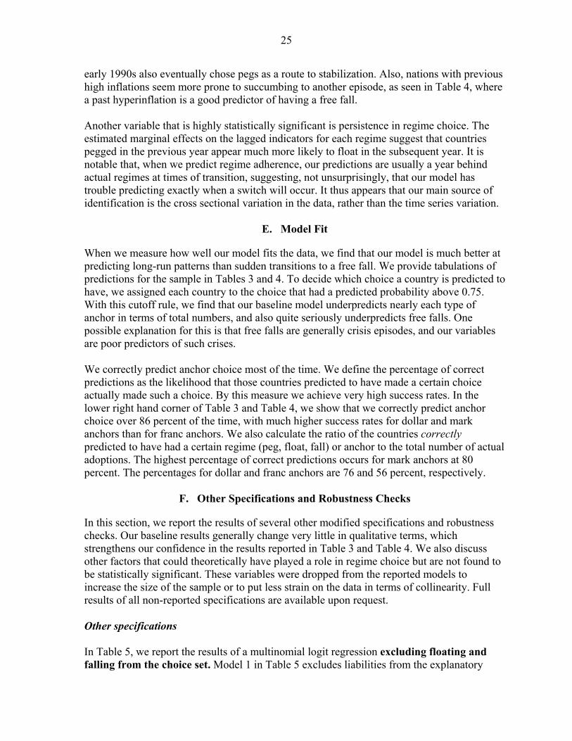
early 1990s also eventually chose pegs as a route to stabilization. Also, nations with previous high inflations seem more prone to succumbing to another episode, as seen in Table 4, where a past hyperinflation is a good predictor of having a free fall. Another variable that is highly statistically significant is persistence in regime choice. The estimated marginal effects on the lagged indicators for each regime suggest that countries pegged in the previous year appear much more likely to float in the subsequent year. It is notable that, when we predict regime adherence, our predictions are usually a year behind actual regimes at times of transition, suggesting, not unsurprisingly, that our model has trouble predicting exactly when a switch will occur. It thus appears that our main source of identification is the cross sectional variation in the data, rather than the time series variation.

E. Model Fit

When we measure how well our model fits the data, we find that our model is much better at predicting long-run patterns than sudden transitions to a free fall. We provide tabulations of predictions for the sample in Tables 3 and 4. To decide which choice a country is predicted to have, we assigned each country to the choice that had a predicted probability above 0.75. With this cutoff rule, we find that our baseline model underpredicts nearly each type of anchor in terms of total numbers, and also quite seriously underpredicts free falls. One possible explanation for this is that free falls are generally crisis episodes, and our variables are poor predictors of such crises. We correctly predict anchor choice most of the time. We define the percentage of correct predictions as the likelihood that those countries predicted to have made a certain choice actually made such a choice. By this measure we achieve very high success rates. In the lower right hand corner of Table 3 and Table 4, we show that we correctly predict anchor choice over 86 percent of the time, with much higher success rates for dollar and mark anchors than for franc anchors. We also calculate the ratio of the countries correctly predicted to have had a certain regime (peg, float, fall) or anchor to the total number of actual adoptions. The highest percentage of correct predictions occurs for mark anchors at 80 percent. The percentages for dollar and franc anchors are 76 and 56 percent, respectively.

F. Other Specifications and Robustness Checks

In this section, we report the results of several other modified specifications and robustness checks. Our baseline results generally change very little in qualitative terms, which strengthens our confidence in the results reported in Table 3 and Table 4. We also discuss other factors that could theoretically have played a role in regime choice but are not found to be statistically significant. These variables were dropped from the reported models to increase the size of the sample or to put less strain on the data in terms of collinearity. Full results of all non-reported specifications are available upon request. Other specifications In Table 5, we report the results of a multinomial logit regression excluding floating and falling from the choice set. Model 1 in Table 5 excludes liabilities from the explanatory

26

variables, while Model 2 includes this variable. In both models, the trade network externality coefficients are positive and statistically significant. The coefficients on the co-movement of output are both negative, although this variable is again not statistically significant for dollar pegs. In Model 2, the currency denomination of liabilities has positive and statistically significant coefficients for both dollar and mark pegs. The past hyperinflation variable is positively related to dollar pegs in both models, but only statistically significant in Model 2. We were unable to estimate the coefficient on past hyperinflation for the mark choice in these reduced samples.

Table 5. Determinants of Anchor Choice, Restricted Choice Set, 1980–1998

Variable dollar mark dollar markTrade with Anchor Bloc 0.171 0.152 0.197 0.137

[0.061]*** [0.048]*** [0.079]** [0.062]**Asymmetry of co-movements w/ anchor GDP -0.051 -0.364 -0.068 -0.616

[0.064] [0.126]*** [0.073] [0.191]***Liabilities payable in Anchor's currency /GDP --- --- 0.184 2.416

[0.040]*** [0.457]***Lagged indicator for past hyperinflation 1.398 --- 3.100 ---

[1.234] [1.305]**Latin America 37.992 --- --- ---

[2.815]***Sub-Saharan Africa -0.581 --- -3.372 ---

[0.981] [1.034]***East Asia Pacific 35.316 --- 57.552 ---

[0.842]*** [8.268]***Eastern/Central Europe --- 2.922 19.034 25.535

[1.736]* [4.348]*** ---Middle East/North Africa 0.133 -1.574 -2.698 -3.077

[1.146] [1.787] [1.284]** [1.616]*Primary Commodity Exporter -1.020 -2.875 0.341 -2.973

[1.170] [1.884] [1.287] [1.558]*Petroleum Exporter -0.909 -33.834 -2.661 -31.346

[1.765] [1.861]*** [2.050] [2.018]***Constant -0.008 1.570 0.957 -0.027

[0.868] [0.876]* [0.752] [1.499]Number of obs

Model 1 Model 2

NOTES: Dependent variable is peg to dollar, franc or mark . Franc peg is the base category. Coefficients are reported above. Heteroscedasticity robust standard errors clustered on countries are in parentheses. Predicted regimes and regime. *** p-value < 0.01; ** p-value < 0.05;* p-value < 0.1

1058 565

In Table 6, we present evidence that endogeneity between trade flows and anchor patterns is not responsible for our previous findings. We use a control function approach recently studied in Ben-Akiva and Guevara (2006). That is, we use a vector of exogenous instruments and the included exogenous regressors to predict trade patterns with the dollar and mark blocs. We then use the residuals from this regression as an explanatory variable in the multinomial logit model. The excluded instrumental variables are the logarithm of great circle distance from the country that issues the anchor currency, the logarithm of population and the interaction between population and distance. These have very high t-statistics in the first stage regressions and, parallel to the argument made by Frankel and Romer (1999), these geographic and demographic variables are seemingly uncorrelated with other omitted factors determining the choice of any particular anchor. Finally, since the exogenous variables are likely to be highly persistent over time, we move to a cross section estimation for 1998.

27

In Table 6, Model 1 excludes the currency denomination of liabilities (liabilities issued in the anchor currency relative to GDP), while Model 2 includes such liabilities. We also present specifications with and without the residuals from a first stage regression side-by-side. In Model 1, we find that endogeneity may have understated the impact of mark trade links for mark pegs. The residual is statistically significant, and when we include it, we find that the coefficient on the mark peg actually becomes larger and is still positive and statistically significant. The coefficient on the dollar trade links does not change much and remains positive and statistically significant. In Model 2, we find some evidence that endogeneity is a problem for the dollar bloc. However, the coefficient on dollar trade links is not statistically significant in either specification of Model 2. Model 2 does not give any indication that trade flows between the mark bloc are endogenous once liability denomination is included. Here the mark trade links are positive and statistically significant. In both specifications of Model 2, liability denomination is positively related to anchor choice and statistically significant. Robustness checks Besides the different specifications, we also carried out five additional robustness checks, the results of which are not reported in the tables but are available upon request. First, we included time dummies in the baseline specification in Table 3. We found that time dummies were jointly significant, although individually they were not. None of the other variables became insignificant when time dummies were included. Moreover, there was only a marginal improvement in fit, as measured by the increase in the likelihood value. Second, as a measure of regional regime popularity, we included the percentage of countries in a region pegging to each anchor currency in a country’s region, instead of including the weighted anchor regime choices of trade partners.29 The benefit of not using the trade-weighted measure of other countries’ regime choice is that we avoid somewhat the endogeneity between trade flows and exchange rate volatility, which arise from the fact that the transaction costs associated with exchange rate volatility may decrease trade (Frankel, 2003). The results were in line with Table 3 and the coefficients on the neighbors’ regimes were even more precisely estimated than the coefficients on trade links from Table 3. A third robustness check we carried out was to re-classify countries so as to exclude some of the more “flexible” pegged regimes from the pegged category. Here, we included countries in the peg column only if they had a fine code smaller than 8 as in Table A1 in Appendix 1. In other words, we no longer considered pre-announced wide crawling bands, wide de facto crawling bands, and moving bands as “pegs”. The results from this exercise were still broadly in line with our baseline. However, while the sign on the volatility of money velocity was found to be positive, as expected, it was not estimated very precisely.

29 We define a region as those countries which border a country and those which are less than 1,800 kilometers measured by great circle distance. As a reference point, Argentina and Brazil are 1707 kilometers apart based on our distance measures. Distance comes from data used in Glick and Rose (2002).

28

Tabl

e 6.

Det

erm

inan

ts o

f Anc

hor C

hoic

e, R

estri

cted

Cho

ice

Set,

1998

Var

iabl

edo

llar

mar

kdo

llar

mar

kdo

llar

mar

kdo

llar

mar

kTr

ade

with

Anc

hor B

loc

0.13

50.

207

0.12

80.

556

0.03

01.

083

-0.1

071.

191

[0.0

51]*

**[0

.058

]***

[0.0

51]*

*[0

.210

]***

[0.0

57]

[0.3

34]*

**[0

.083

][0

.380

]***

Trad

e w

ith A

ncho

r Blo

c 'R

esid

uals

' --

- --

--0

.016

-0.5

25 --

- --

-0.

168

-0.0

26[0

.071

][0

.226

]**

[0.0

91]*

[0.1

29]

Asy

mm

etry

of c

o-m

ovem

ents

w/ a

ncho

r GD

P0.

009

-0.3

050.

009

-0.4

710.

007

-0.8

390.

007

-0.9

21[0

.008

][0

.137

]**

[0.0

07]

[0.1

48]*

**[0

.006

][0

.245

]***

[0.0

05]

[0.2

77]*

**Li

abili

ties

paya

ble

in A

ncho

r's c

urre

ncy

/GD

P --

- --

- --

- --

-0.

537

9.48

20.

594

10.2

97[0

.162

]***

[2.7

64]*

**[0

.193

]***

[3.2

30]*

**E

aste

rn/C

entra

l E

urop

e --

-2.

955

---

2.36

6 --

-1.

612

---

2.57

2[1

.629

]*[1

.444

][1

.070

][1

.572

]M

iddl

e E

ast/N

orth

Afri

ca-0

.269

-1.6

91-0

.242

-1.9

19-1

.374

-24.

912

-2.1

04-2

7.23

0[0

.884

][1

.783

][0

.873

][1

.392

][1

.281

][7

.515

]***

[1.4

87]

[8.7

57]*

**P

rimar

y C

omm

odity

Exp

orte

r-1

.285

-2.1

29-1

.294

-3.6

95-1

.348

-66.

613

-1.5

75-7

1.57

5[0

.782

][1

.632

][0

.768

]*[1

.568

]**

[0.8

95]

[19.

742]

***

[0.9

14]*

[17.

501]

***

Con

stan

t0.

026

0.42

50.

035

-2.0

26-0

.616

-23.

693

0.71

3-2

5.89

5[0

.623

][1

.054

][0

.704

][2

.011

][0

.648

][7

.573

]***

[0.8

77]

[8.7

12]*

**

Num

ber o

f obs

Mod

els

with

Lia

bilit

ies

NO

TES

: Dep

ende

nt v

aria

ble

is p

eg to

dol

lar,

franc

or m

ark.

The

fran

c pe

g is

the

base

cat

egor

y. C

oeffi

cien

ts a

re re

porte

d. H

eter

osce

dast

icty

robu

st s

tand

ard

erro

rs a

re in

pa

rent

hese

s. E

ndog

enei

ty s

peci

ficifi

catio

ns (M

odel

s 2

and

2A) i

nclu

de th

e re

sidu

als

from

a fi

rst s

tage

regr

essi

on o

f tra

de li

nks

on th

e lo

garit

hm o

f dis

tanc

e fro

m th

e an

chor

cou

ntry

, the

log 80

Mod

el 1

Mod

el 1

(End

ogen

eity

con

trol)

Mod

el 2

8282

80

of p

opul

atio

n, a

n in

tera

ctio

n of

the

popu

latio

n an

d di

stan

ce v

aria

bles

and

oth

er in

clud

ed e

xpla

nato

ry v

aria

bles

. ***

p-v

alue

< 0

.01;

**

p-va

lue

< 0.

05; *

p-v

alue

< 0

.1

Mod

el 2

(End

ogen

eity

con

trol)

29

We also estimated a fourth specification that included the choice to use the pound sterling as an anchor. As is evident in Figure 1, sterling declined a lot in popularity beginning in the 1960s. The story of sterling’s decline in popularity as an anchor currency is more complex than what one regression can capture, and there are of course many individual country experiences combined with political factors. Still, the declining stability of monetary policy in Britain and hence the impact on the pound/dollar exchange rate is arguably a key reason why countries might have preferred other anchors to the pound. Another factor was the fear of large losses on sterling balances (i.e., sterling reserves) due to depreciation. This forced a move to diversify reserve assets and hence helped lead to other anchor choices. This episode might be evidence of a self-reinforcing dynamic, arising from the strategic complementarities we outlined above as a partial explanation for why fewer and fewer countries have chosen a sterling peg over the long-run.30 When we estimated a specification similar to that in Table 4, but included the pound as an anchor choice, we found evidence that the choice for a pound anchor was positively associated with the volume of trade with the sterling area.31 Finally, we checked robustness to excluding developed countries from our sample. However, there was little evidence that the factors driving anchor choice in this case are different than for the full sample.

G. Other Factors that Appear Less Relevant or Are Hard to Test

There are three factors that we did not include because they appeared last relevant or were hard to test. These are (1) the denomination of foreign currency deposits; (2) political variables; and (3) the degree of competition. Similar to the currency denomination of liabilities, the denomination of foreign currency deposits would seem to be a natural additional important determinant of anchor currency choice. That is, just as countries may want to anchor their exchange rate to “hedge” the exchange rate risk associated with foreign currency denominated liabilities, they may want to do the same for foreign currency denominated assets. Unfortunately, we lack sufficient high-quality data for a broad sample to include this variable in our study, but we feel that it might be a contributing factor, as the literature has noted. To the extent that countries that have suffered past hyperinflations are those that tend to have a dollarized banking system, our coefficient on past hyperinflations could be picking up this effect. Political variables were also difficult to include because of data limitations. Since the exchange rate regime is normally a political decision, it could certainly be the case that

30 Reinhart and Rogoff’s data reveal the following information about certain transitions from the pound to the dollar: (1) Australia and New Zealand simultaneously adopted a dollar anchor in 1972; (2) the East Caribbean Central Bank States (Antigua and Barbuda, Anguilla, Dominica, Grenada, Montserrat, Saint Kitts and Nevis, Saint Lucia, Saint Vincent and the Grenadines) all went to the dollar at once in 1976; (3) Iraq, Kuwait, and Jordan also adopted their dollar anchors almost simultaneously in 1972; and (4) Myanmar (1975), Sri Lanka (1976), Hong Kong (1972), Malaysia (1976), Pakistan (1972), and Singapore (1972) all moved to the dollar at nearly the same time. 31 We do not report these results, because data limitations forced us to drop other variables in this specification.

30

political interests and institutions affect the observed outcomes. For example, we could imagine a political economy model of anchor currency choice, where interest groups with trade links with a given bloc will exert pressure on politicians to decrease their transaction costs of trade by implementing a peg. The literature has also argued that institutions and interests are important (Bernhard and Leblang, 1999). We tried using a Herfindahl index of political parties to measure how likely the system is to give rise to a government with homogeneous interests. We also tried an ex post measure of government stability which gauges the turnover in veto players during a given period. Finally, we tried using the percentage of seats held in the legislative assembly by the government as a measure of the strength of the actual governing party. These political data came from the Database of Political Institutions.32 While none of the political economy variables we included in our estimations showed up as statistically significant, this is not to say that political constraints do not matter. The data we used are limited and imperfect indicators and cover a much smaller sub-sample. More work could go into the theoretical and empirical exploration of how these factors might influence de facto regimes. Finally, in the context of the literature on optimal pegs, Dornbusch and Park (1999) and Kwan (1994) discuss the issues of competition and output stabilization. Such arguments rely on intimate knowledge of the level of pass-through, the invoicing practices, the direction of trade and the actual level of competition at the aggregate level. Such considerations are interesting as potential anchor determinants but seem daunting in terms of finding appropriate controls, and even more difficult for policy makers to consider. Moreover, such prescriptions seem to us more normative than positive in nature.

VII. CONCLUSION

Virtually all countries that have chosen to peg their currencies in some way to another currency have converged over the last fifty years to using either the U.S. dollar or the euro as anchors for those pegs. This raises a number of important questions: Why have some countries chosen to peg their currency to the U.S. dollar while others have chosen to peg to the euro? Why are other currencies no longer popular as anchors? And more generally, what determines the choice of anchor currency in a pegged (or nearly pegged) exchange rate regime? In this paper, we studied the determinants of anchor currency choice as well as the determinants of the choice to peg itself. Using a new dataset on de facto exchange rate regimes and a multinomial logit framework, we presented evidence that a key factor explaining the convergence to euro (mark and franc) and dollar anchors is the existence of trade network externalities. These arise because the payoffs of using a particular anchor increase with the amount of trade with countries that use the same anchor. Indeed, our empirical results show that the choice of a particular anchor depends positively on the

32Frankel (2003) suggests that symmetry in political preferences between the anchor country and the pegging country may make it easier to generate a political consensus about the right way to adjust to such a shock. How to control for such symmetry is an interesting question that we leave for further research.

31

amount of trade with countries that use that anchor. Moreover, we find that, if trade were to exogenously increase with those countries pegging to, for example, the euro, it would be individually optimal for these countries to switch to a euro anchor. Our results are thus consistent with an “optimal anchor currency area theory,” i.e., the optimal currency area theory applied to anchor currency choice. We also find that two other factors matter for anchor currency choice. First, countries that experience business cycles that are similar to those of an anchor-issuing country are more likely to adopt that particular anchor. Second, countries that have liabilities denominated in a certain currency are more likely to adopt that currency as an anchor for their peg. Regarding the factors that determine whether countries choose to peg in the first place, as opposed to float, our results are generally in line with previous empirical studies of regime choice. Size seems to be the principal determinant, with larger countries being less likely to peg. Like in other studies, our results here do not seem very robust. This is consistent with Juhn and Mauro’s (2002) finding that there are no robust empirical regularities that determine how countries choose their exchange rate regimes. Two important lessons emerge about the geography of the international monetary system based on the study of anchor choice. First, countries can be locked into a suboptimal equilibrium. If a large number of countries are pegging to a certain currency, then, in the absence of a large crisis, or another unanticipated extreme event, it may be difficult to break out of this pattern into another perhaps more socially beneficial set of arrangements. If a suboptimal equilibrium is reached, the associated use of the suboptimally chosen anchor currency in international transactions and as a reserve currency implies that this anchor currency may become overvalued. This, in turn, may give rise to an unsustainably large current account deficit in the anchor currency issuing country, which some would argue has happened in the United States (for example, Obstfeld and Rogoff, 2004; and Eichengreen, 2004). Second, small changes in anchor choices can have large and rapid effects on the geography of the international monetary system. For example, when the demand for assets denominated in an overvalued anchor currency begins to fall, as may be the case with the U.S. dollar as of mid-2007, this could induce a critical number of countries to switch anchors, or adopt a float, and may eventually allow other anchoring countries to break out of the suboptimal equilibrium. This, in turn, may be associated with a sudden decrease in the willingness of nonresidents to continue funding ongoing trade deficits, and potentially to a currency crisis. This would not be the first time in history that a currency bloc has unraveled in this way. The sudden demise of silver and bimetallic standards in the 1870s and of the sterling bloc in the 1970s illustrate that such dynamics are a real possibility in the future.

32

APPENDIX I: THE NATURAL CLASSIFICATION The data The Reinhart and Rogoff natural classification puts exchange rate regimes into fifteen fine and six coarse categories as summarized above. The classification is based on monthly data on official and market-determined exchange rates for the period 1946-2001.33 The market-determined exchange rate data come from various issues of Pick’s Currency Yearbook, Pick’s Black Market Yearbooks, and Pick’s World Currency Report and the official rate comes from the same sources as well as from the IMF. The quotes are end-of-month exchange rates and are not subject to revisions. For the countries that had one or more monetary reforms, involving changes in the units in which the exchange rate is expressed, the data has been converted as necessary to ensure continuity. For more information see Rogoff et. al. (2004) and Reinhart and Rogoff (2004). Table A1. Regime Classification Codes and Descriptions. fine course Description 1 1 No separate legal tender 2 1 Pre announced peg or currency board arrangement 3 1 Pre announced horizontal band that is narrower than or equal to +/-2% 4 1 De facto peg 5 2 Pre announced crawling peg 6 2 Pre announced crawling band that is narrower than or equal to +/-2% 7 2 De factor crawling peg 8 2 De facto crawling band that is narrower than or equal to +/-2% 9 3 Pre announced crawling band that is wider than or equal to +/-2% 10 3 De facto crawling band that is narrower than or equal to +/-5% 11 3 Moving band that is narrower than or equal to +/-2% (i.e., allows for

both appreciation and depreciation over time) 12 3 Managed floating 13 4 Freely floating 14 5 Freely falling 15 6 Dual market in which parallel market data is missing

33 In some instances, the data for the market-determined rates are available for a shorter period. Observations where the parallel market was known to be substantial but parallel rate data were not available were marked “unclassified.”

33

APPENDIX II. A MODEL OF TRADE NETWORK EXTERNALITIES IN ANCHOR CURRENCY CHOICE

In this Appendix, we show formally why network externalities in anchor choice can lead to multiple equilibria. We do this by considering a simple two-currency two-country model with simple deterministic payoffs, which we then generalize to multiple countries with stochastic and anchor-specific payoffs. Two country model with deterministic payoffs Suppose initially that the world consists of only two countries, i and j, and each country has a choice between two anchor currencies: the U.S. dollar ($) and the euro (€). The payoffs (Ui, Uj) associated with each anchor currency choice are given in Table B1.

Table B1. Simple Payoff Matrix

Aj = $ Aj = €

Ai = $ 1,1 0,0

Ai = € 0,0 1,1

When the two countries each choose a different anchor currency, they both face transaction costs that depend on the bilateral exchange rate volatility between the euro and the dollar. We normalize the payoffs associated with this volatility to zero. When the two countries both adopt the same anchor currency, they are able to reduce this bilateral exchange rate volatility (and hence transaction costs), and these savings are represented by a payoff value of one. The optimal strategy, or best response, for each country is, therefore, to do what the other country does, i.e., Ai =Aj and Aj =Ai. This implies two Nash equilibria in pure strategies: one where both countries adopt the dollar, and one where both adopt the euro as their anchor. Multiple country model Now suppose that each country has multiple trade partners, where the share of each trade partner in total trade is denoted by tij=Tij/Ti, with Tij denoting the total amount of trade between countries i and j, and Ti denoting the total amount of trade between country i and the rest of the world. For simplicity, we assume that all positive bilateral exchange rate volatilities generate zero payoffs (this assumption can be generalized later), and that zero bilateral exchange rate volatility (i.e., adopting the same anchor as a trade partners) generates payoffs equal to 1/J, where J is the number of trade partners. This implies that the payoff to country i of adopting a given anchor currency increases in the number of countries that adopt the same anchor currency, and these payoffs equal one if all trade partners adopt the same anchor. Alternatively, the trade share tij can be interpreted as the probability that the next international transaction between country i and the rest of the world takes place with country j. The expected payoff of adopting an anchor currency Ai is then:

34

1

( ) ( , )J

i i ij i i jj

U A t U A A=

= ∑ .

Since we assume, for now, that ( , ) 0,i i jU A A i j= ∀ ≠ , this can be alternatively written as

1

( ) ( )J

i i ij j ij

U A t I A A=

= =∑ ,

where I(Aj=Ai) is an indicator function that equals one when j adopts the same anchor currency as i, and zero otherwise. Thus, the payoff for country i associated with using anchor currency A is simply the weighted average (weighted by trade shares) of the number of trade partners that use this same anchor currency. In particular,

1($) ( $) Pr( $) ($)

J

i ij j j jj

U t I A A p=

= = = = ≡∑ ,

that is, the payoff for country i of anchoring to the dollar equals the share of i’s trade that takes place with dollar-anchoring countries. In terms of our two-country game, this trade share can be interpreted as the probability that the “representative trade partner” is anchored to the dollar. Similarly, we can write

1

(€) ( €) Pr( €) 1 ($)J

i ij j j jj

U t I A A p=

= = = = ≡ −∑ ,

Deterministic payoffs In a deterministic model, i.e., without any idiosyncratic preferences, the best response for country i can then be written as follows:

0 if ($) 0.5($) [0,1] if ($) 0.5

= 1 if ($) 0.5

j

i j

j

pp p

p

⎧ = <⎪∈ =⎨⎪ >⎩

This best response correspondence is illustrated in Figure A1. It implies that country i will choose to anchor to the dollar if there is more than a 50 percent chance that the representative trade partner j will anchor to the dollar as well, i.e., if more than half of its trade partners are anchored to the dollar (the “dollar bloc”). Conversely, country i will anchor to the euro if the representative trade partner j is most likely to anchor to the euro, i.e., if the majority of trade partners are anchored to the “euro bloc”. When exactly half of its trade is with the dollar bloc, and half of its trade with the euro bloc, country i is indifferent between the two anchor currencies and chooses an anchor at random.

35

Figure A1. Equilibria of the Deterministic Anchor Choice Model

Proposition 1: Equilibria of the deterministic anchor choice model (Figure A1) Suppose that all countries are identical except for their trade shares (i.e., there are no other determinants of anchor currency choice besides trade network externalities). Then, (a) there exist three symmetric Nash equilibria, one with all countries pegging to the dollar, one with all countries pegging to the euro, and one with all countries randomizing between dollar and euro (resulting in half the world pegging to the dollar and half the world pegging to the euro); (b) asymmetric Nash equilibria can exist only when the world is split into two or more separate trade blocs (closed subsets), so that within each bloc, all countries trade with each other, but there is no trade between any two countries from different blocs.

Proof: (a) In a symmetric Nash equilibrium, pi($) = pj($) = p($). Suppose that all countries except i are pegged to the dollar. Then country i’s best response is to peg to the dollar as well, i.e., p($)=1 is a Nash equilibrium. Similarly, when all trade partners of i are pegged to the euro, i’s best response is to peg to the euro as well, i.e., p($)=0 is a Nash equilibrium. Finally, suppose all countries randomize between pegging to the dollar and pegging to the euro. Then the expected share of the dollar bloc is 50 percent independently of trade patterns, hence, under rational expectations, the best response is to randomize between dollar and euro, i.e., p($)=0.5 is a Nash equilibrium. (b) Since there is no trade between the trade blocs, it follows from (a) that it is possible for each trade bloc to settle on a different symmetric Nash equilibrium (different currency blocs).

0

0.5

1

0 0.5 1Probability that i adopts $

Prob

abili

ty th

at j

ado

pts $

36

Country-specific payoffs Next, consider the more general, non-deterministic case with idiosyncratic, country-specific preferences εi(Ai). We can then write

($) ($) ($)i j iU p με= + (€) (€) (€)i j iU p με= + ,

where μ is a parameter to denote the relative importance of country-specific preferences. This gives the following best response function:

($) Pr( ($) ($) (€) (€))

1Pr( ($) (€) [ ($) (€)])

2Pr( ($) (€) [ ($) 0.5])

i j i j i

i i j j

i i j

p p p

p p

p

με με

ε εμ

ε εμ

= + > +

= − < − −

= − < − −

,

where the last equation results from the fact that

(€) 1 ($).j jp p= −

Note that, for μ=0, this equation reduces to the best response correspondence given above. A standard assumption in discrete choice models is that the idiosyncratic term is a random variable which is exponentially distributed. This gives a logit model:

1 2[ ($) (€)] [ ($) 0.5]

1 1($) ,1 1

j j ji

p p pp

e eμ μ− − − −

= =

+ +

For μ→0, the best response correspondence reduces to that of the deterministic model (without idiosyncratic preferences). Proposition 2: Equilibria of the stochastic anchor choice model (Figure A2) Suppose that all countries are identical except for sensitivity to trade network externalities. Defining a symmetric equilibrium as pi($) = pj($) = p($), we hold that: (a) for μ>0.5, there exists a unique symmetric Nash equilibrium, with p($)=0.5 (b) for μ<0.5, there exist two additional symmetric Nash equilibria: one equilibrium where the majority of countries are pegging to the dollar, i.e., p($)>0.5, and one equilibrium where the majority of countries are pegging to the euro, i.e., p($)<0.5. Proof: It can easily be verified that p($)=0.5 is always an equilibrium, and that, for μ=0.5, the slope of the best response function in this equilibrium equals unity, i.e., pi'($)=1 at pi($)=0.5. For μ>0.5, the slope is less than unity, i.e., pi' ($)<1 at pi($)=0.5, which implies that there is a unique symmetric equilibrium. For μ<0.5, the slope exceeds unity, which implies the

37

existence of three symmetric equilibria. We omit a formal proof here, which is given in Oomes (2003b), and instead illustrate this proposition in Figure A2.34

Figure A2. Equilibria of the Stochastic Anchor Choice Model

For Different Values of μ

The best response functions and equilibria of the stochastic model are illustrated in Figure A2 for various values of μ. Intuitively, when μ is relatively small, idiosyncratic factors are not very important, and hence the model is similar to the deterministic model, where network externalities are the only determinants of anchor currency choice, and generate three symmetric equilibria. However, when μ is large, idiosyncratic factors start to play a more important role than network externalities, and therefore the multiple equilibria disappear. Generalized country-specific payoffs The case with general payoffs ( , )i i jU A A and ( , )j i jU A A and idiosyncratic, country-specific preferences is shown in Table B2. For simplicity we still assume that there are only two anchor currencies, but the results can be generalized to n anchor currencies.

Table B2. Generalized Payoff Matrix

Aj = $ Aj = €

Ai = $ Ui($,$),Uj($,$) Ui($,€),Uj($,€)

Ai = € Ui(€,$),Uj(€,$) Ui(€,€),Uj(€,€)

34 Oomes (2003b) also shows that it is possible for asymmetric equilibria to exist for local trade networks, where every country trades only with its neighbors, but is indirectly able to trade with any other country. In addition, Oomes (2003b) shows that the threshold value of μ depends on the extent of home bias: for low home bias (or high trade openness), the threshold is never reached, and there is always a unique symmetric equilibrium,

0

0.5

1

0 0.5 1probability that i adopts $

prob

abili

ty th

at j

adop

ts $

μ =0.5μ =0.3

μ =1

38

In this case, the best response function generalizes to ($)

($) (€) (€) ($)

1($)1

i

i i i i

U

i U U U U

epe e e −= =

+ +,

with

($) ($) ($,$) (€) ($, €) ($)i j i j i iU p U p U με= + +

(€) ($) (€,$) (€) (€, €) (€)i j i j i iU p U p U με= + +

($) (€) ($)[ ($,$) (€,$)] (€)[ ($, €) (€, €)] [ ($) (€)]i i j i i j i i i iU U p U U p U U μ ε ε− = − + − + −

In other words, country i’s relative payoffs of pegging to the dollar instead of the euro,

($) (€)i iU U− , depend on how much better it is for i to peg to the dollar when j also pegs to

the dollar, i.e. ($,$) (€,$)i iU U− , and how much better (or worse) it is for i to peg to the

dollar when j pegs to the euro, i.e., ($, €) (€, €)i iU U− .

Using the fact that (€) 1 ($)j jp p= − , we can rewrite the above expression as

($) (€) ($) ( ($) (€)),i i j i iU U pα β μ ε ε− = + + −

where

[ ($,$) ($, €)] [ (€, €) (€,$)];[ ($, €) (€, €)].

i i i i

i i

U U U UU U

βα= − + −= −

This gives

1 [ ($)]

1($)1

ji

pp

eα β

μ− +

=

+

,

where we can see that the simple payoff matrix above was a special case, with α=-1 and β=2.The parameter β can be interpreted as a measure of the strength of network externalities. When β>0, network externalities are positive, since the probability that a given country adopts a dollar anchor increases with the probability that its “random trade partner” is anchored to the dollar, which equals the share of i’s trade that takes place with dollar-anchoring countries. When β<0, network externalities are negative, since the probability of pegging to the dollar decreases with the share of trade with dollar-anchoring countries. When β=0, network externalities are absent, since the slope of the best response function is zero. In this case, we have

($,$) (€,$) ($, €) (€, €)i i i iU U U U− = − ,

39

which means that the relative payoffs of pegging to the dollar are the same regardless of the anchor choices by trade partners. Country-specific and anchor-specific payoffs In Figure A3, we illustrate how our model is affected by the existence of anchor-specific payoffs. The dark bold line going through the point (0.5,0.5) is an example of a best response function for the model without anchor-specific payoffs, which as we have shown exhibits multiple equilibria if idiosyncratic preferences are not too strong. Now suppose that the euro becomes to be considered a more stable currency than the dollar, e.g., in terms of the level and variability of inflation. This would not affect β, but it would affect α = Ui($,€)−Ui(€,€), which measures the relative payoffs of pegging to the dollar given a particular trade partner anchor choice. Intuitively, when euro-specific payoffs exist, the probability of pegging to the dollar decreases independently of how popular the dollar is among trade partners (i.e., independently of the size of network externalities). This means that the best response function shifts downwards. Similarly, the existence of dollar-specific payoffs implies that the best response function shifts upwards. As Figure A3 shows, a sufficiently large downward shift of the best response function (which occurs when euro-specific payoffs exceed dollar-specific payoffs) implies that the multiple equilibria disappear and that there is only one unique equilibrium left, in which the majority of countries peg to the euro. Similarly, a sufficiently large upward shift of the best response function (which occurs when dollar-specific payoffs dominate) implies that the majority of countries will end up pegging to the dollar .

Figure A3. Equilibria of the Stochastic Anchor Choice Model With Anchor-Specific Payoffs

0

0.5

1

0 0.5 1

Probability that i adopts $

Prob

abili

ty th

at j

ado

pts $

40

REFERENCES

Alesina, Alberto, and Alexander Wagner, 2006, “Choosing (and Reneging on) Exchange Rate Regimes.” Journal of the European Economics Association, Vol. 4, pp. 770–799.

Arthur, W. Brian, 1989, “Competing Technologies, Increasing Returns, and Lock-In by

Historical Events.” Economic Journal, Vol. 99, pp. 116–131. Bayoumi, Tamim, and Barry Eichengreen, 1999, “Is Asia an Optimum Currency Area? Can

It Become One? Regional, global and historical perspectives on Asian monetary relations.” In: Exchange Rate Policies in Emerging Asian Countries. Routledge. Collignon, Stefan, Jean Pisani-Ferry, and Yung Chul Park, eds., London, pp. 347–365.

Bayoumi, Tamim, and Barry Eichengreen, 1997, “Ever Closer to Heaven? An Optimum

Currency Area Index for European Countries.” European Economic Review Papers and Proceedings, Vol.41, pp. 761–70.

Bernhard, William, and David Leblang, 1999, “Democratic Institutions and Exchange-rate

Commitments.” International Organization, Vol. 53(1), pp. 71–97. Beck, Nathaniel, David, Epstein, Simon Jackman, and Sharyn O’ Halloran, 2002,

“Alternative Models of Dynamics in Binary Time-Series-Cross Section Models: The Example of State Failure.” Unpublished working paper, Stanford University, Palo Alto, California.

__________, Jonathan Katz, and Richard Tucker, 1998, “Taking Time Seriously: Time-

Series–Cross-Section Analysis with a Binary Dependent Variable.” American Journal of Political Science, Vol. 42 (4), pp. 1260–1288.

Beck, Thorsten, George Clarke, Alberto Groff, Philip Keefer, and PatrickWalsh, 2001, “New

Tools in Comparative Political Economy: The Database of Political Institutions.” World Bank Economic Review, Vol. 15 (1), pp.165–176.

Ben-Akiva, Moshe E., and Cristian Angleo Guevara, 2006, “Endogeneity in Residential

Location Choice Models.” Transportation Research Record: Journal of the Transportation Research Board No. 1977, pp. 60–66.

Bubula, Andrea, and İnci,Ötker-Robe, 2002, “The Evolution of Exchange Rate Regimes

Since 1990: Evidence From De Facto Policies,” IMF Working Paper 02/155 (Washington: International Monetary Fund).

Calvo, Guillermo A., and Carmen M., Reinhart, 2002, “Fear of Floating.” Quarterly Journal

of Economics, Vol. 117 (2), pp. 379–408.

41

Camdessus, Michel, 1995. The Dollar, The Yen and European Currencies. Address at the XIV Sesiones de Trabajo de Tesoreria, Caja de Ahorros de Navarra, Pamplona, Spain, November 17, 1995. International Monetary Fund, Washington, DC.

Cuddington, John T., and Samuel K. Otoo, 1990, “Choice of Exchange Rate Regime: A

Multinomial Logit Model.” Unpublished Working Paper No. 90-18,Georgetown University, Washington, D.C.

Dornbusch, Rudiger, and Yung Chul Park, 1999, “Flexibility or Nominal Anchors?” In:

Exchange Rate Policies in Emerging Asian Countries. Collignon, Stefan, Jean, Pisani-Ferry, and Yung Chul Park, eds., Routledge, London, pp. 3-34.

Dowd, Kevin, and David Greenaway, 1993, “Currency Competition, Network Externalities

and Switching Costs: Towards an Alternative View of Optimum Currency Areas.” Economic Journal, Vol. 103 (127), pp. 1180–1189.

Dreyer, Jacob S., 1978, “Determinants of Exchange Rate Regimes for Currencies of

Developing Countries: Some Preliminary Results.” World Development, Vol. 6, 437–445.

East Caribbean Economic and Financial Review. June 1976. 7 (1), 12-29. (??) Edwards, Sebastian, 1996, “The Determinants of the Choice Between Fixed and Flexible

Exchange-Rate Regimes.” NBER Working Paper No. 5756 (Cambridge, Massachusetts: MIT Press).

Eichengreen, Barry, and Marc Flandreau, 1998. “The Geography of the Gold Standard.” In:

Currency Convertibility: The Gold Standard and Beyond. Braga de Macedo, Jorge, Barry Eichengreen, and Jaime Reis, eds. Routledge, London, pp. 113–143.

Eichengreen, Barry, and Donald J. Mathieson, 2000, “The Currency Composition of Foreign

Exchange Reserves: Retrospect and Prospect.” IMF working paper No. 00/131 (Washington: International Monetary Fund).

____________, 2004, “Global Imbalances and the Lessons of Bretton Woods.” NBER

Working Paper No. 10497 (Cambridge, Massachusetts: MIT Press). Fasano, Ugo, and Andrea Schaechter, 2003, Monetary Union Among Member Countries of

the Gulf Cooperation Council. IMF Occasional Paper No. 223 (Washington: International Monetary Fund).

Flandreau, Marc, 1996, “The French Crime of 1873: An Essay in the Emergence of the

International Gold Standard, 1870-1880.” Journal of Economic History, Vol. 56 (4), pp. 862-897.

42

Frankel, Jeffrey A., and David Romer, 1999, “Does Trade Cause Growth?” The American Economic Review, Vol. 89 (3), pp. 379–399.

Frankel, Jeffrey A., 2003, “Experience of and Lessons from Exchange Rate Regimes in

Emerging Economies.” NBER Working Paper No. 10032. (Cambridge, Massachusetts: MIT Press).

Frieden, Jeffry, Piero Ghezzi, and Ernesto Stein, 2005, “Politics and Exchange Rates: A

Cross-Country Approach to Latin America.” Journal of Applied Economics, Vol. 8 (2), pp. 203–225.

Ghosh, Atish, Anne-Marie Gulde, Jonathan Ostry, and Holger Wolf, 1997, “Does the

Nominal Exchange Rate Regime Matter?” NBER Working Paper, No. 5874 (Cambridge, Massachusetts: MIT Press)

Glick, Reuven, and Andrew K. Rose, 2002, “Does a Currency Union Affect Trade? The

Time-Series Evidence.” European Economic Review, Vol. 46 (6), pp. 1125–1151. Goodhart, Charles, 1989, “The Conduct of Monetary Policy.” Economic Journal, Vol. 99

(396), pp. 293–346. Hausmann, Ricardo, Ugo Panizza, Ernesto Stein, 2001, “Why Do Countries Float the Way

They Float?” Journal of Development Economics, Vol. 66, pp. 387–414. Heller, H. Robert, 1978, “Determinants of Exchange Rate Practices.” Journal of Money,

Credit and Banking, Vol. 10, pp. 308–21. Holden, Merle, Paul Holden, and Esther Suss, 1979, “The Determinants of Exchange Rate

Flexibility: An Empirical Investigation.” Review of Economics and Statistics, Vol. 61 (3), pp. 327–333.

Iwami, Toru, 1994, “The Internationalization of Yen and Key Currency Questions.” IMF

Working Paper No. 94/41 (Washington: International Monetary Fund). Juhn, Grace, Paolo Mauro, 2002,. “Long-Run Determinants of Exchange Rate Regimes: A

Simple Sensitivity Analysis.” IMF Working Paper No. 02/104 (Washington:International Monetary Fund).

Kenen, Peter B., and Ellen E. Meade, 2006, “Monetary Integration in East Asia.” In:

Regional Monetary Integration, Kenen, Peter B., and Ellen E. Meade, eds. Cambridge University Press, New York.

Klein, Michael W., and Jay C. Shambaugh, 2006, “Fixed Exchange Rates and Trade.”

Journal of International Economics, Vol. 70, pp. 359–383.

43

Kiyotaki, Nobuhiro, and Randall Wright, 1989, “On Money as a Medium of Exchange.” Journal of Political Economy, Vol. 97 (4), pp. 927–954.

Kouri, Pentti J.K., Braga de Macedo, Jorge, 1978. Exchange Rates and the International

Adjustment Process, Brookings Papers on Economic Activity, 1, 111-1150. Kraft, Vajur, 1999, “Why a Fixed Rate and the CB?” Speech given at Helsinki Seminar on

the Accession Process. Available via the Internet : http://213.180.8.164/pub/en/dokumendid/publikatsioonid/seeriad/koned/varasem/_1998-1999/ar9911102.html?objId=963338

Krugman, Paul, 1984, “The International Role of the Dollar: Theory and Prospect.” In:

Exchange Rate Theory and Practice, Bilson, John F.O., and Richard C. Marston, eds., National Bureau of Economic Research and University of Chicago Press, Chicago, pp. 261–280.

___________, 1979, “A model of balance of payments crises.” Journal of Money, Credit,

and Banking, Vol. 11, pp. 311–325. Kwan, C.H, 1994, “Economic Interdependence in the Asia-Pacific Region: Towards a yen

Bloc.” The Brookings Institution and Routledge, New York. Kwan, C.H, 2001, “Yen Bloc: Toward Economic Integration in East Asia.” The Brookings

Institution and Routledge, New York Levy-Yeyati, Eduardo, and Federico Sturzenegger, 2003. “A De Facto Classification of

Exchange Rate Regimes: A Methodological Note.” American Economic Review, Vol. 93 (4). Available at http://www.aeaweb.org/aer/contents

____________, Federico Sturzenegger, and Eliana Reggio, 2003, “On the Endogeneity of

Exchange Rate Regimes.” Unpublished Working Paper Universidad Torcuato di Tella, Argentina.

Maddala, G. S., 1987, “Limited Dependent Variable Models Using Panel Data.” The Journal

of Human Resources, Vol. 22 (3), pp. 305–338. Masson, Paul, 2001, “Exchange Rate Regime Transitions.” Journal of Development

Economics, Vol. 64 (2), pp. 571-586. ____________, and Catherine Pattillo, 2005, The Monetary Geography of Africa

(Washington: Brookings Institution Press). McKibbin, Warwick J., and Hong-Giang Lee, 2004, “Which Exchange Rate Regime for

Asia?” Brookings Discussion Papers in International Economics, No. 158, Washington, D.C.

44

Meissner, Christopher M., 2005, “A New World Order: Explaining the International Diffusion of the Gold Standard, 1870-1913.” Journal of International Economics, Vol. 66, pp. 385–406.

Obstfeld, Maurice, and Kenneth Rogoff, 2004, “The Unsustainable U.S. Current Account

Position Revealed.” NBER Working Paper, No. 10869 (Cambridge, Massachusetts: MIT Press)

___________, and Alan M. Taylor, 1998, “The Great Depression as a Watershed:

International Capital Mobility in the Long Run.” In: The Defining Moment: The Great Depression and the American Economy in the Twentieth Century. Bordo, Michael, Claudia, D. Goldin, and Eugene N. White, eds. University of Chicago Press, Chicago.

Ogawa, Eiji, and Takatoshi Ito, 2000, “On the Desirability of a Regional Currency Basket.”

NBER Working Paper No. 8002 (Cambridge, Massachusetts: MIT Press). Poirson, Hélène, 2001, “How Do Countries Choose Their Exchange Rate Regime?” IMF

Working Paper No. 01/46 (Washington: International Monetary Fund). Reinhart, Carmen, and Kenneth Rogoff, 2004, “The Modern History of Exchange Rate

Arrangements: A Reinterpretation.” Quarterly Journal of Economics, Vol. 119 (1), pp. 1–48.

_____________, 2003, “The Country Chronologies and Chartbook. Background Material to

A Modern History of Exchange Rate Arrangements: A Reinterpretation. Part I”. Available via the Internet: http://www.publicpolicy.umd.edu/faculty/reinhart/PartI_Chronologies.pdf

Rizzo, Jean-Marc, 1998, “The Economic Determinants of the Choice of an Exchange Rate

Regime: A Probit Analysis.” Economics Letters, Vol. 59 (3), pp. 283–287. Rogoff, Kenneth, Aasim Husain, Ashoka Mody, Robin Brooks, and Nienke Oomes, 2004.

“Evolution and Performance of Exchange Rate Regimes.” IMF Working Paper No. 03/243. (Washington: International Monetary Fund).

Shambaugh, Jay C, 2004, “The Effect of Fixed Exchange Rates on Monetary Policy.”

Quarterly Journal of Economics, Vol. 119 (1), pp. 301–352. Savvides, Andreas, 1990, “Real Exchange Rate Variability and the Choice of Exchange Rate

Regime by Developing Countries.” Journal of International Money and Finance, Vol.9, pp. 440–454.

Tavlas, George S., and Yuzuri Ozeki, 1992, The Internationalization of Currencies: An

Appraisal of the Japanese Yen, IMF Occasional Paper No. 90 (Washington: International Monetary Fund).

45

Veyrune, Romain, 2007, “Fixed Exchange Rates and the Autonomy of Monetary Policy: The Franc Zone Case.” IMF Working Paper No. 07/34. (Washington: International Monetary Fund).

WAMI News, 2002, European Central Bank and WAMI Hold Workshop on Monetary Union

in West Africa 10-15, April. West African Monetary Institute, Accra. WAMI News, 2003, Preliminary Study Report on Banking Supervision in the WAMZ 10–

11, August. West African Monetary Institute, Accra. Worrell, DeLisle, Dona Marshall, and Nicole Smith, 2000, “The Political Economy of

Exchange Rate Policy in the Caribbean.” Inter-American Development Bank Working Paper Vo. R-401, Washington, D.C.

Yehoue, Etienne B., 2004, “Currency Bloc Formation as a Dynamic Process Based on Trade

Network Externalities,” IMF Working Paper No. 04/222 (Washington: International Monetary Fund).

Yehoue, Etienne B., 2006, “On the Pattern of Currency Blocs in Africa,” Journal of African

Development, Volume 1, No 1, pp. 39–86.