why do life insurance policyholders lapse? the roles of
TRANSCRIPT
Why Do Life Insurance Policyholders Lapse?
The Roles of Income, Health and Bequest Motive Shocks∗
Hanming Fang† Edward Kung‡
May 2, 2010
Abstract
We present an empirical dynamic discrete choice model of life insurance decisions designed
to bypass data limitations where researchers only observe whether an individual has made a
new life insurance decision but but do not observe the actual policy choice or the choice set
from which the policy is selected. The model also incorporates serially correlated unobservable
state variables, for which we provide ample evidence that they are required to explain some
key features in the data. We empirically implement the model using the limited life insurance
holding information from the Health and Retirement Study (HRS) data. We deal with seri-
ally correlated unobserved state variables using posterior distributions of the unobservables
simulated from Sequential Monte Carlo (SMC) methods. Counterfactual simulations using the
estimates of our model suggest that a large fraction of life insurance lapsations are driven by
i.i.d choice specific shocks, particularly when policyholders are relatively young. But as the
remaining policyholders get older, the role of such i.i.d. shocks gets less important, and more
of their lapsations are driven either by income, health or bequest motive shocks. Income and
health shocks are relatively more important than bequest motive shocks in explaining lapsa-
tions when policyholders are young, but as they age, the bequest motive shocks play a more
important role.
Keywords: Life insurance lapsations, Sequential Monte Carlo Method
JEL Classification Codes: G22, L11
∗Preliminary and Incomplete. All comments are welcome. We have received helpful comments and suggestionsfrom Han Hong, Aprajit Mahajan, Jim Poterba and Ken Wolpin. Fang would also like to gratefully acknowledge thegenerous financial support from the National Science Foundation through Grant SES-0844845. All remaining errors areour own.†Department of Economics, University of Pennsylvania, 3718 Locust Walk, Philadelphia, PA 19104; Duke University
and the NBER. Email: [email protected]‡Department of Economics, Duke University, 213 Social Sciences Building, P.O. Box 90097, Durham, NC 27708-0097.
Email: [email protected]
1 Introduction
The life insurance market is large and important. Policyholders purchase life insurance to pro-
tect their dependents against financial hardship when the insured person, the policyholder, dies.
According to Life Insurance Marketing and Research Association International (LIMRA Interna-
tional), 78 percent of American families owned some type of life insurance in 2004. By the end
of 2008, the total number of individual life insurance policies in force in the United States stood
at about 156 million; and the total individual policy face amount in force reached over 10 trillion
dollars (see American Council of Life Insurers (2009, p. 63-74)).
There are two main types of individual life insurance products, Term Life Insurance and Whole
Life Insurance.1 A term life insurance policy covers a person for a specific duration at a fixed or
variable premium for each year. If the person dies during the coverage period, the life insurance
company pays the face amount of the policy to his/her beneficiaries, provided that the premium
payment has never lapsed. The most popular type of term life insurance has a fixed premium
during the coverage period and is called Level Term Life Insurance. A whole life insurance policy,
on the other hand, covers a person’s entire life, usually at a fixed premium. In the United States at
year-end 2008, 54 percent of all life insurance policies in force is Term Life insurance. Of the new
individual life insurance policies purchased in 2008, 43 percent, or 4 million policies, were term
insurance, totaling $1.3 trillion, or 73 percent, of the individual life face amount issued (see Ameri-
can Council of Life Insurers (2009, p. 63-74)). Besides the difference in the period of coverage, term
and whole life insurance policies also differ in the amount of cash surrender value (CSV) received
if the policyholder surrenders the policy to the insurance company before the end of the coverage
period. For term life insurance, the CSV is zero; for whole life insurance, the CSV is typically
positive and pre-specified to depend on the length of time that the policyholder has owned the
policy. One important feature of the CSV on whole life policies relevant to our discussions below
is that by government regulation, CSVs does not depend on the health status of the policyholder
when surrendering the policy.2
Lapsation is an important phenomenon in life insurance markets. Both LIMRA and Society of
Actuaries considers that a policy lapses if its premium is not paid by the end of a specified time
(often called the grace period). This implies that if a policyholder surrenders his/her policy for
1The Whole Life Insurance has several variations such as Universal Life (UL) and Variable Life (VL) and Variable-Universal Life (VUL). Universal Life allows varying premium amounts subject to a certain minimum and maximum.For Variable Life, the death benefit varies with the performance of a portfolio of investments chosen by the policyholder.Variable-Universal Life combines the flexible premium options of UL with the varied investment option of VL (seeGilbert and Schultz, 1994).
2The life insurance industry typically thinks of the CSV from the whole life insurance as a form of tax-advantagedinvestment instrument (see Gilbert and Schultz, 1994).
1
1998 1999 2000 2001 2002 2003 2004 2005 2006 2007 2008
By Face Amount 8.3 8.2 9.4 7.7 8.6 7.6 7.0 6.6 6.3 6.4 7.6
By Number of Policies 6.7 7.1 7.1 7.6 9.6 6.9 7.0 6.9 6.9 6.6 7.9
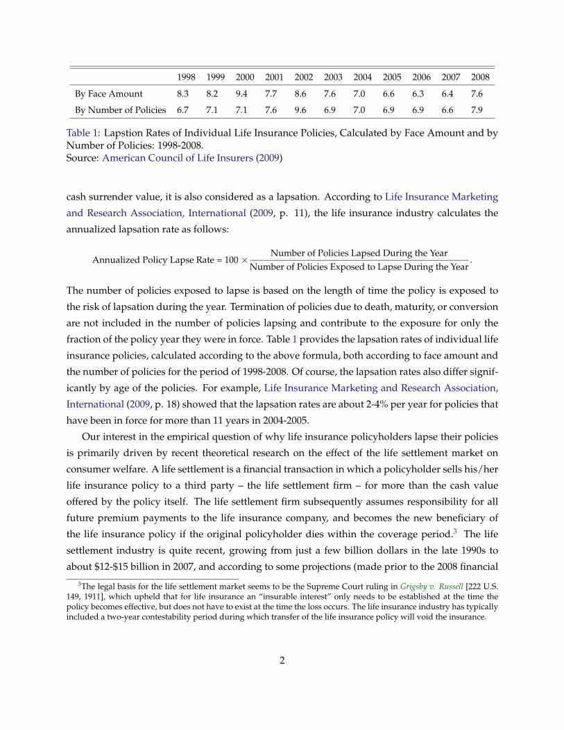
Table 1: Lapstion Rates of Individual Life Insurance Policies, Calculated by Face Amount and byNumber of Policies: 1998-2008.Source: American Council of Life Insurers (2009)
cash surrender value, it is also considered as a lapsation. According to Life Insurance Marketing
and Research Association, International (2009, p. 11), the life insurance industry calculates the
annualized lapsation rate as follows:
Annualized Policy Lapse Rate = 100 × Number of Policies Lapsed During the YearNumber of Policies Exposed to Lapse During the Year
.
The number of policies exposed to lapse is based on the length of time the policy is exposed to
the risk of lapsation during the year. Termination of policies due to death, maturity, or conversion
are not included in the number of policies lapsing and contribute to the exposure for only the
fraction of the policy year they were in force. Table 1 provides the lapsation rates of individual life
insurance policies, calculated according to the above formula, both according to face amount and
the number of policies for the period of 1998-2008. Of course, the lapsation rates also differ signif-
icantly by age of the policies. For example, Life Insurance Marketing and Research Association,
International (2009, p. 18) showed that the lapsation rates are about 2-4% per year for policies that
have been in force for more than 11 years in 2004-2005.
Our interest in the empirical question of why life insurance policyholders lapse their policies
is primarily driven by recent theoretical research on the effect of the life settlement market on
consumer welfare. A life settlement is a financial transaction in which a policyholder sells his/her
life insurance policy to a third party – the life settlement firm – for more than the cash value
offered by the policy itself. The life settlement firm subsequently assumes responsibility for all
future premium payments to the life insurance company, and becomes the new beneficiary of
the life insurance policy if the original policyholder dies within the coverage period.3 The life
settlement industry is quite recent, growing from just a few billion dollars in the late 1990s to
about $12-$15 billion in 2007, and according to some projections (made prior to the 2008 financial
3The legal basis for the life settlement market seems to be the Supreme Court ruling in Grigsby v. Russell [222 U.S.149, 1911], which upheld that for life insurance an “insurable interest” only needs to be established at the time thepolicy becomes effective, but does not have to exist at the time the loss occurs. The life insurance industry has typicallyincluded a two-year contestability period during which transfer of the life insurance policy will void the insurance.
2
crisis), is expected to grow to more than $150 billion in the next decade (see Chandik, 2008).4
In recent theoretical research, Daily, Hendel and Lizzeri (2008) and Fang and Kung (2010a)
showed that, if policyholders’ lapsation is driven by their loss of bequest motives, then consumer
welfare is unambiguously lower with life settlement market than without. However, Fang and
Kung (2010b) showed that if policyholders’ lapsation is driven by income or liquidity shocks,
then life settlement may potentially improve consumer welfare. The reason for the difference in
the welfare result is as follows. Life insurance is typically a long-term contract with one-sided
commitment in which the life insurance companies commit to a typically constant stream of pre-
mium payments whereas the policyholder can lapse anytime. Because the premium profile is
typically constant, the contracts are typically front-loaded, that is, in the early part of the policy
period, the premium payments exceed the actuarially fair value of the risk insured. In the later
part of the policy period, the premium payments are less than the actuarially fair value. As a
result, whenever a policyholder lapses his/her policy after holding it for several periods, the life
insurance company pockets the so-called lapsation profits, which is factored into the pricing of the
life insurance policy to start with due to competition. The key effect of the settlement firms on the
life insurers is that the settlement firms will effectively take away the lapsation profits, forcing the
life insurers to adjust the policy premiums and possibly the whole structure of the life insurance
policy under the consideration that lapsation profits do not exist. In the theoretical analysis, we
show that life insurers may respond to the threat of life settlement by limiting the degree of re-
classification risk insurance, which certainly reduces consumer welfare. However, the settlement
firms are providing cash payments to policyholders when the policies are sold to the life settle-
ment firms. The welfare loss from the reduction in extent of reclassification risk insurance has
to be balanced against the welfare gain to the consumers when they receive payments from the
settlement firms when their policies are sold. If policyholders sell their policies due to income
shocks, then the cash payments are received at a time of high marginal utility of income, and the
balance of the two effects may result in a net welfare gain for the policyholders. If policyholders
sell their policies as a result of losing bequest motives, the balance of the two effects on net result in
a welfare loss. Thus, to inform policy-makers on how the emerging life settlement market should
be regulated, an empirical understanding of why policyholders lapse is of crucial importance.
For this purpose, we present and empirically implement a dynamic discrete choice model of
life insurance decisions. The model is “semi-structural” and is designed to bypass data limitations
4The life settlement industry actively targets wealthy seniors 65 years of age and older with life expectancies from 2to up to 12-15 years. This differs from the earlier viatical settlement market developed during the 1980s in response tothe AIDS crisis, which targeted persons in the 25-44 age band diagnosed with AIDS with life expectancy of 24 monthsor less. The viatical market largely evaporated after medical advances dramatically prolonged the life expectancy of anAIDS diagnosis.
3
where researchers only observe whether an individual has made a new life insurance decision (i.e.,
purchased a new policy, or added to/changed an existing policy) but do not observe what the ac-
tual policy choice is nor the choice set from which the new policy is selected. We empirically
implement the model using the limited life insurance holding information from the Health and
Retirement Study (HRS) data. An important feature of our model is the incorporation of seri-
ally correlated unobservable state variables. In our empirical analysis, we show ample evidence
that such serially correlated unobservable state variables are important for explaining some key
features in the data.
Methodologically, we deal with serially correlated unobserved state variables using posterior
distributions of the unobservables simulated from Sequential Monte Carlo (SMC) methods.5 Rel-
ative to the few existing papers in the economics literature that have used similar SMC methods,
our paper is, to the best of our knowledge, the first to incorporate multi-dimensional serially cor-
related unobserved state variables. In order to give the three unobservable state variables in our
empirical model their desired interpretations as unobserved income, health and bequest motive
shocks, this paper proposes two channels through which we can anchor these unobservables to
their related observable variables.
Our estimates for the model with serially correlated unobservable state variables are sensible
and yield implications about individuals’ life insurance decisions consistent with the both intu-
ition and existing empirical results. In a series of counterfactual simulations reported in Table 15,
we find that a large fraction of life insurance lapsations are driven by i.i.d choice specific shocks,
particularly when policyholders are relatively young. But as the remaining policyholders get
older, the role of such i.i.d. shocks gets less important, and more of their lapsations are driven
either by income, health or bequest motive shocks. Income and health shocks are relatively more
important than bequest motive shocks in explaining lapsation when policyholders are young, but
as they age, the bequest motive shocks play a more important role.
The remainder of the paper is structured as follows. In section 2 we describe the data set
used in our empirical analysis and how we constructed key variables, and we also provide the
descriptive statistics. In Section 3 we describe the empirical model of life insurance decisions.
In section 4 we provide some preliminary reduced-form and static structural models describing
the relationship between life insurance decisions and individuals’ observable characteristics. In
section 5 we expand the model to explicitly account for dynamics, and we use counterfactual
simulations to investigate the effects of income and bequest shocks to lapsation patterns. In section
5See also Norets (2009) which develops a Bayesian Markov Chain Monte Carlo procedure for inference in dynamicdiscrete choice models with serially correlated unobserved state variables. Kasahara and Shimotsu (2009) and Hu andShum (2009) present the identification results for dynamic discrete choice models with serially correlated unobservablestate variables.
4
6 we extend the dynamic model to include serially correlated unobserved state variables, and
describe a method to account for them in estimation. In Section 7 we report our counterfactual
experiments using the model with unobservables. In section 8 we conclude.
2 Data
We use data from the Health and Retirement Study (HRS). The HRS is a nationally representa-
tive longitudinal survey of older Americans which began in 1992 and has been conducted every
two years thereafter. The HRS is particularly well suited for our study for two reasons. First, the
HRS contains rich information about income, health, family structure, and life insurance owner-
ship. If family structure can be interpreted as a measure of bequest motive, then we have all the
key factors motivating our analysis. Second, the HRS respondents are generally quite old: be-
tween 50 to 70 years of age in their first interview. As we described in the introduction, the life
settlements industry typically targets policyholders in this age range or older, so it is precisely the
lapsation behavior of this group that we are most interested in.
Our original sample consists of 4,512 male respondents who were successfully interviewed in
both the 1994 and 1996 HRS waves, and who were between the ages of 50 and 70 in 1996. We
chose 1996 as the period to begin decision modeling because starting in 1996 the HRS began to
ask questions about whether or not the respondent lapsed any life insurance policies and whether
or not the respondent obtained any new life insurance policies since the last interview. These
questions are used in the construction of the decision variable in the structural model. We use
only respondents who were also interviewed in 1994 so we can know whether or not they owned
life insurance in 1994.
We follow these respondents until 2006. Any respondent who missed an interview for any
reason other than death between 1996 and 2006 was dropped from the sample. Any respondent
with a missing value on life insurance ownership any time during this period was also dropped.
This leaves us a sample of 3,567 males. We also dropped 243 individuals who never reported
owning life insurance during all the waves of HRS data. Our final analysis sample thus consists of
3,324 in wave 1996 and the survivors among them in subsequent waves, 3,195 in wave 1998, 3022
in wave 2000, 2,854 in wave 2002, 2,717 in wave 2004 and 2,558 in wave 2006. Table 2 describes
how we come to our final estimation sample.
Construction of Variables Related to Life Insurance Decisions. Except for the variables related
to life insurance decision, all other variables used in our analysis are taken directly from the
RAND distribution of the HRS. Here we describe the questions in HRS we use to construct the
5

Table 2: Sample Selection Criterion and Sample Size
Selection Criterion Sample Size
All individuals who responded to both 1994 and 1996 HRS interviews 17,354
... males who were aged between 50 and 70 in 1996 (wave 3) 4,512
... did not having any missing interviews from 1994 to 2006 3,696
... did not have any missing values for reported life insurance ownership status from 1994 to 2006 3,567
... reported owning life insurance at least once from 1996 to 2006 3,324
Note: The selection criteria are cumulative.
life-insurance related variables.
∙ For whether or not an individual owned life insurance in the current wave, we use the indi-
vidual’s response to the following HRS survey question, which is asked in all waves:
[Q1] “Do you currently have any life insurance?”
∙ For whether or not an individual obtained a policy since the previous wave, we use the
individual’s response to the following HRS question, which is asked all waves starting in
1996:
[Q2] “Since (previous wave interview month-year) have you obtained any new life insurance
policies?”
If the respondent answers “yes,” we consider him to have obtained a new policy.
∙ For whether or not an individual lapsed a policy since last wave, we use the individual’s
response to the following HRS question:
[Q3] “Since (previous wave interview month-year) have you allowed any life insurance poli-
cies to lapse or have any been cancelled?”
We also use the response to another survey question:
[Q4] “Was this lapse or cancellation something you chose to do, or was it done by the
provider, your employer, or someone else?”
If the respondent answers “yes” to the first question and answers “my decision” to the sec-
ond question, we consider him to have lapsed a policy.
In the notation of the model we presented in the previous section, we construct an individual’s
period-t (or wave- t) decisions as follows:
6

∙ For the individual who reported not having life insurance in the previous wave (dt−1 = 0),
we let dt = 0 if the individual reports not having life insurance this wave; and dt = 1 if
the individual reports having life insurance this wave (“yes” to Q1). Because the individual
does not own life insurance in period t − 1 but does in period t, we interpret that he chose
the optimal policy in period t given his state variables at t.
∙ For the individual who reported having life insurance in the previous wave (dt−1 > 1), we
let dt = 0 if the individual reports not having life insurance this wave (“no” to Q1). We let
dt = 1 (i.e. the individual re-optimizes his life insurance) if the individual reports having life
insurance this wave (“yes” to Q1) and he obtained new life insurance policy (“yes” to Q2),
OR if the individual answered “yes” to Q1, reported lapsing (i.e. answered “yes” to Q3) and
reported that lapse was his own decision (answered “my own decision” to Q4). Note that
under this construction, we have interpreted the “lapsing or obtaining” of any policies as an
indication that the respondent re-optimized his life insurance coverage. Finally, we let dt = 2
(i.e. he kept his previous life insurance policy unchanged) if the individual reports having
life insurance this wave (“yes” to Q1) and the individual did not report yes to obtaining new
policy (“no” to Q2) and the individual did not lapse any existing policy (either report “no”
to Q3 or reported “yes” to Q3 but did not report “my decision” to Q4).
Information About the Details of Life Insurance Holdings in the HRS Data. HRS also has
questions regarding the face amount and premium payments for life insurance policies. However,
there are several problems with incorporating these variables into our empirical analysis. First,
the questions differ across waves. In the 1994 wave, questions were asked regarding total face
amount and premium for term life policies; but for whole life policies only total face amount was
collected.6 From 2000 on, the HRS asked about the combined face value for all policies, combined
face value for whole life policies, and the combined premium payments for whole life policies.
Note that the premium for term life policies were not collected from 2000 on. Second, there is
a very high incidence of missing data regarding life insurance premiums and face amounts. In
our selected sample, 40.3% of our selected sample (1340 individuals) have at least one instance of
missing face amount in waves when he reported owning life insurance. The incidence of missing
values in premium payments is even higher. Third, even for those who reported face amount
and premium payments for their life insurance policies, we do not know the choice set they faced
when purchasing their policies.
6The questions in 1994 wave related to premium and face amount are: [W6768]. About how much do you pay for(this term insurance/these term insurance policies) each month or year? [W6769]. Was that per month, year, or what?[W6770]. What is the current face value of all the term insurance policies that you have? [W6773]. What is the currentface value of (this [whole life] policy/these [whole life] policies?)
7
For these reasons, we decide to only model the individuals’ life insurance decisions regard-
ing whether to re-optimize, lapse or maintaining an existing policy, and only use the observed
information about the above decisions in estimating the model.
2.1 Descriptive Statistics
Patterns of Life Insurance Coverage and its Transitions. Table 3 provides the life insurance
coverage and patterns of transition between coverage and no coverage in the HRS data. Panel A
shows that among the 3,324 live respondents in 1996, 88.1% are covered by life insurance; among
the 3,195 who survived to the 1998 wave, 85.7% owned life insurance, etc. Over the waves, the life
insurance coverage rates among the live respondents seem to exhibit a declining trend, with the
coverage rate among the 2,558 who survived to the 2006 wave being about 78.6%.
Panel B and C show, however, that there are substantial transition between the coverage and no
coverage. Panel B shows that among the 512 individuals who did not have life insurance coverage
in 1994, almost a half (47.5%) obtained coverage in 1996; in later waves between 25.6% to 33.7%
of individuals without life insurance in the previous wave ended up with coverage in the next
wave. Panel C shows that there is also substantial lapsation among life insurance policyholders.
In our data, between-wave lapsation rates range from 4.6% to 10.2%. Considering that our sample
is relatively old and the tenures of holding life insurance policies in the HRS sample are also
typically longer, these lapsation rates are in line with the industry lapsation rates reported in the
introduction (see Table 1).
Panel D shows that even among those individuals who own life insurance in both the previous
wave and the current wave, a substantial fraction has changed the face amount of their coverage,
or in the words of our model, re-optimized. Between 6.0% to 9.5% of the sample who have insur-
ance coverage in adjacent waves reported changing the face amount of their coverages by their
“own decisions”.
Summary Statistics of State Variables, by Life Insurance Coverage Status. Table 4 summarizes
the key state variables for the sample used in our empirical analysis. It shows that the average
age of the live respondents in our sample is 61.1, which increases by less than two years in the next
waves. This is as expected, because those who did not survive to the next wave because of death
tend to be older than average. The mean of log household income in our sample is quite stable
around 10.58 to 10.73, with slight increase over the waves, possibly because low income individ-
uals tend to die earlier. The next six rows report the mean of the incidence of health conditions,
including high blood pressure, diabetes, cancer, lung disease, heart disease and stroke. It shows
clear signs of health deterioration for the surviving samples over the years. The sum of the above
8

Table 3: Life Insurance Coverage and Transition Patterns in HRS: 1996-2006
Wave
1996 1998 2000 2002 2004 2006
Panel A: Life Insurance Coverage Status
Currently covered by life insurance 2,927 2,739 2,524 2,313 2,187 2,011
88.1% 85.7% 83.5% 81.0% 80.5% 78.6%
No life insurance coverage 397 456 498 541 530 547
11.9% 14.3% 16.5% 19.0% 19.5% 21.4%
Total live respondents 3,324 3,195 3,022 2,854 2,717 2,558
Panel B: Life Insurance Coverage Status
Conditional on No Coverage in Previous Wave
Life insurance coverage this wave 243 125 130 150 163 123
47.5% 33.4% 31.9% 33.7% 32.7% 25.6%
No life insurance coverage this wave 269 249 277 295 336 357
52.5% 66.6% 68.1% 66.3% 67.3% 74.4%
Total live respondents with no coverage last wave 512 374 407 445 499 480
Panel C: Life Insurance Coverage Status
Conditional on Coverage in Previous Wave
Life insurance coverage this wave 2,684 2,614 2,394 2,163 2,024 1,888
95.4% 92.7% 91.5% 89.8% 91.3% 90.9%
No life insurance coverage this wave 128 207 221 246 194 190
4.6% 7.3% 8.5% 10.2% 8.7% 9.1%
Total respondents with coverage last wave 2,812 2,821 2,615 2,409 2,218 2,078
Panel D: Whether Changed Coverage Amount Conditional
on Coverage in Both Current and Previous Waves
Did not change coverage amount 2,430 2,395 2,233 2,034 1,881 1,769
90.5% 91.6% 93.3% 94.0% 92.9% 93.7%
Changed coverage amount 254 219 161 129 143 119
9.5% 8.4% 6.7% 6.0% 7.1% 6.3%
Total live respondents with coverage in both waves 2,684 2,614 2,394 2,163 2,024 1,888
9

Tabl
e4:
Sum
mar
ySt
atis
tics
ofSt
ate
Var
iabl
es.
Var
iabl
eD
escr
ipti
onW
ave
1996
1998
2000
2002
2004
2006
Age
ofre
spon
dent
61.1
0163
.035
64.9
2466
.851
68.7
8870
.676
(4.3
53)
(4.3
43)
(4.3
06)
(4.2
85)
(4.2
85)
(4.2
50)
Log
hous
ehol
din
com
e10
.581
10.5
8610
.623
10.6
1110
.688
10.7
26
(1.3
01)
(1.2
08)
(1.2
05)
(1.2
04)
(1.0
38)
(0.9
15)
Whe
ther
ever
diag
nose
dw
ith
high
bloo
dpr
essu
re0.
4025
0.43
720.
4768
0.51
750.
5686
0.62
00
(0.4
90)
(0.4
96)
(0.4
99)
(0.5
00)
(0.4
95)
(0.4
85)
Whe
ther
ever
diag
nose
dw
ith
diab
etes
0.14
380.
1593
0.17
570.
2064
0.22
750.
2525
(0.3
51)
(0.3
66)
(0.3
81)
(0.4
05)
(0.4
19)
(0.4
35)
Whe
ther
ever
diag
nose
dw
ith
canc
er0.
0599
0.08
110.
1006
0.12
860.
1590
0.18
73
(0.2
37)
(0.2
73)
(0.3
00)
(0.3
35)
(0.3
66)
(0.3
90)
Whe
ther
ever
diag
nose
dw
ith
lung
dise
ase
0.07
130.
0782
0.07
970.
0886
0.10
890.
1177
(0.2
57)
(0.2
68)
(0.2
71)
(0.2
84)
(0.3
12)
(0.3
22)
Whe
ther
ever
diag
nose
dw
ith
hear
tdis
ease
0.19
010.
2144
0.23
490.
2670
0.30
470.
3432
(0.3
92)
(0.4
10)
(0.4
24)
(0.4
42)
(0.4
60)
(0.4
75)
Whe
ther
ever
diag
nose
dw
ith
stro
ke0.
0493
0.05
790.
0652
0.07
110.
0828
0.09
85
(0.2
17)
(0.2
34)
(0.2
47)
(0.2
57)
(0.2
76)
(0.2
98)
Whe
ther
ever
diag
nose
dw
ith
psyc
holo
gica
lpro
blem
0.06
010.
0717
0.07
910.
0876
0.09
350.
1005
(0.2
38)
(0.2
58)
(0.2
70)
(0.2
83)
(0.2
91)
(0.3
01)
Whe
ther
ever
diag
nose
dw
ith
arth
riti
s0.
3904
0.44
600.
4831
0.53
110.
5793
0.62
08
(0.4
88)
(0.4
97)
(0.5
00)
(0.4
99)
(0.4
94)
(0.4
85)
Sum
ofab
ove
cond
itio
ns1.
3676
1.54
591.
6952
1.89
802.
1244
2.34
05
(1.2
41)
(1.2
92)
(1.3
11)
(1.3
37)
(1.3
95)
(1.4
21)
Whe
ther
mar
ried
0.85
020.
8429
0.84
410.
8444
0.84
360.
8323
(0.3
57)
(0.3
64)
(0.3
63)
(0.3
63)
(0.3
63)
(0.3
74)
#of
live
resp
onde
nts
3,32
43,
195
3,02
22,
854
2,71
72,
558
Not
e:St
anda
rdde
viat
ions
are
inpa
rent
hesi
s.
10

Tabl
e5:
Sum
mar
ySt
atis
tics
ofSt
ate
Var
iabl
esC
ondi
tion
alon
Hav
ing
Life
Insu
ranc
e
Var
iabl
eD
escr
ipti
onW
ave
1996
1998
2000
2002
2004
2006
Age
ofre
spon
dent
61.0
7062
.989
64.8
3966
.825
68.7
6570
.688
(4.3
39)
(4.3
23)
(4.3
18)
(4.2
84)
(4.3
11)
(4.2
60)
Log
hous
ehol
din
com
e10
.689
10.7
0010
.714
10.6
9010
.754
10.7
79
(1.1
56)
(1.0
81)
(1.0
90)
(1.1
30)
(0.9
47)
(0.8
57)
Whe
ther
ever
diag
nose
dw
ith
high
bloo
dpr
essu
re0.
3980
0.43
560.
4794
0.52
100.
5697
0.61
46
(0.4
90)
(0.4
96)
(0.5
00)
(0.5
00)
(0.4
95)
(0.4
87)
Whe
ther
ever
diag
nose
dw
ith
diab
etes
0.13
260.
1475
0.16
160.
1937
0.21
630.
2392
(0.3
39)
(0.3
55)
(0.3
68)
(0.3
95)
(0.4
12)
(0.4
27)
Whe
ther
ever
diag
nose
dw
ith
canc
er0.
0591
0.07
920.
1010
0.13
450.
1632
0.19
14
(0.2
36)
(0.2
70)
(0.3
01)
(0.3
41)
(0.3
70)
(0.3
93)
Whe
ther
ever
diag
nose
dw
ith
lung
dise
ase
0.06
870.
0748
0.07
730.
0865
0.10
400.
1144
(0.2
53)
(0.2
63)
(0.2
67)
(0.2
81)
(0.3
05)
(0.3
18)
Whe
ther
ever
diag
nose
dw
ith
hear
tdis
ease
0.18
450.
2107
0.23
380.
2655
0.30
500.
3431
(0.3
88)
(0.4
08)
(0.4
23)
(0.4
42)
(0.4
61)
(0.4
75)
Whe
ther
ever
diag
nose
dw
ith
stro
ke0.
0430
0.05
180.
0590
0.06
440.
0759
0.09
10
(0.2
03)
(0.2
22)
(0.2
36)
(0.2
46)
(0.2
65)
(0.2
88)
Whe
ther
ever
diag
nose
dw
ith
psyc
holo
gica
lpro
blem
0.04
990.
0632
0.06
690.
0774
0.08
640.
0919
(0.2
18)
(0.2
43)
(0.2
50)
(0.2
67)
(0.2
81)
(0.2
89)
Whe
ther
ever
diag
nose
dw
ith
arth
riti
s0.
3898
0.43
920.
4774
0.53
570.
5812
0.62
36
(0.4
88)
(0.4
96)
(0.5
00)
(0.4
99)
(0.4
93)
(0.4
85)
Sum
ofab
ove
cond
itio
ns1.
3256
1.50
201.
6565
1.87
852.
1015
2.30
93
(1.2
06)
(1.2
61)
(1.3
00)
(1.3
32)
(1.3
77)
(1.3
95)
Whe
ther
mar
ried
0.87
190.
8638
0.85
940.
8591
0.86
190.
8458
(0.3
34)
(0.3
43)
(0.3
48)
(0.3
48)
(0.3
45)
(0.3
61)
#of
live
resp
onde
nts
wit
hlif
ein
sura
nce
cove
rage
2,92
72,
739
2,52
42,
313
2,18
72,
011
Not
e:St
anda
rdde
viat
ions
are
inpa
rent
hesi
s.
11

Tabl
e6:
Sum
mar
ySt
atis
tics
ofSt
ate
Var
iabl
esC
ondi
tion
alon
Not
Hav
ing
Life
Insu
ranc
e
Var
iabl
eD
escr
ipti
onW
ave
1996
1998
2000
2002
2004
2006
Age
ofre
spon
dent
61.3
3063
.307
65.3
5766
.965
68.8
8770
.629
(4.4
48)
(4.4
54)
(4.2
19)
(4.2
90)
(4.1
75)
(4.2
16)
Log
hous
ehol
din
com
e9.
790
9.90
510
.162
10.2
7310
.418
10.5
35
(1.9
05)
(1.6
37)
(1.5
91)
(1.4
31)
(1.3
16)
(1.0
81)
Whe
ther
ever
diag
nose
dw
ith
high
bloo
dpr
essu
re0.
4358
0.44
740.
4639
0.50
280.
5642
0.63
99
(0.4
96)
(0.4
98)
(0.4
99)
(0.5
00)
(0.4
96)
(0.4
80)
Whe
ther
ever
diag
nose
dw
ith
diab
etes
0.22
670.
2302
0.24
690.
2606
0.27
360.
3016
(0.4
19)
(0.4
21)
(0.4
32)
(0.4
39)
(0.4
46)
(0.4
59)
Whe
ther
ever
diag
nose
dw
ith
canc
er0.
0654
0.09
210.
0984
0.10
350.
1415
0.17
18
(0.2
48)
(0.2
89)
(0.2
98)
(0.3
05)
(0.3
49)
(0.3
78)
Whe
ther
ever
diag
nose
dw
ith
lung
dise
ase
0.09
070.
0987
0.09
240.
0980
0.13
020.
1298
(0.2
88)
(0.2
99)
(0.2
90)
(0.2
98)
(0.3
37)
(0.3
36)
Whe
ther
ever
diag
nose
dw
ith
hear
tdis
ease
0.23
170.
2368
0.24
100.
2736
0.30
380.
3437
(0.4
22)
(0.4
26)
(0.4
28)
(0.4
46)
(0.4
60)
(0.4
75)
Whe
ther
ever
diag
nose
dw
ith
stro
ke0.
0957
0.09
430.
0964
0.09
980.
1113
0.12
61
(0.2
94)
(0.2
93)
(0.2
95)
(0.3
00)
(0.3
15)
(0.3
32)
Whe
ther
ever
diag
nose
dw
ith
psyc
holo
gica
lpro
blem
0.13
600.
1228
0.14
060.
1312
0.12
260.
1316
(0.3
43)
(0.3
29)
(0.3
48)
(0.3
38)
(0.3
28)
(0.3
38)
Whe
ther
ever
diag
nose
dw
ith
arth
riti
s0.
3955
0.48
680.
5120
0.51
200.
5717
0.61
06
(0.4
89)
(0.5
00)
(0.5
00)
(0.5
00)
(0.4
95)
(0.4
88)
Sum
ofab
ove
cond
itio
ns1.
6776
1.80
921.
8916
1.98
152.
2189
2.45
52
(1.4
34)
(1.4
38)
(1.3
50)
(1.3
57)
(1.4
63)
(1.5
07)
Whe
ther
mar
ried
0.69
010.
7171
0.76
710.
7819
0.76
790.
7824
(0.4
63)
(0.4
51)
(0.4
23)
(0.4
13)
(0.4
23)
(0.4
13)
#of
live
resp
onde
nts
wit
hout
life
insu
ranc
eco
vera
ge39
745
649
854
153
054
7
Not
e:St
anda
rdde
viat
ions
are
inpa
rent
hesi
s.
12
six health conditions steadily increase from 1.37 in 1996 to 2.34 in 2006. Finally, the marital status
of the surviving sample seems to be quite stable, with the fraction married being in the range of
83% to 85%.
Tables 5 and 6 summarize the mean and standard deviation of the state variables by the life
insurance coverage status. There does not seem to be much of a difference in ages between those
with and without life insurance coverage, but the mean log household income is significantly
higher for those with life insurance than those without. Moreover, those with life insurance tend
to be healthier than those without life insurance, and they are much more likely to be married
than those without.
3 An Empirical Model of Life Insurance Decisions
In this section we present a discrete choice model of how individuals make life insurance
decisions. We will later implement the dynamic structural model. Our model is simple, yet rich
enough to capture the dynamic intuition behind the life insurance models of Hendel and Lizzeri
(2003) and Fang and Kung (2010a).
Time is discrete and indexed by t = 1, 2, ... In the beginning of each period t, an individual i
either has or does not have an existing life insurance policy. If the individual enters period t with-
out an existing policy, then he chooses between not owning life insurance (dit = 0) or optimally
purchasing a new policy (dit = 1). If the individual enters period t with an existing policy, then,
besides the above two choices, he can additionally choose to keep his existing policy (dit = 2). If
an individual who has life insurance in period t− 1 decides not to own life insurance in period t,
we interpret it as lapsation of coverage. As we describe in Section 2, the choice dit = 1 for an indi-
vidual who previously owns a policy is interpreted more broadly: an individual is considered to
have re-optimized his existing policy if he reported purchasing a new policy or choosing to lapse
an existing policy. The key intrepretation for choice dit = 1 is that the individual re-optimized his
life insurance holdings.
Flow Payoffs from Choices. Now we describe an individual’s payoffs from each of these choices.
First, let xit ∈ X denote the vector of observable state variables of individual i in period t, and let
zit ∈ Z denote the vector of unobservable state variables.7 These characteristics include variables
that affect the individual’s preference for or cost to owning life insurance, such as income, health
and bequest motives. We normalize the utility from not owning life insurance (i.e., dit = 0)to 0;
7We present the model here assuming the presence of both the observed and unobserved state variables. In Section 5,we will also estimate a model with only observed state variables. In that case, we should simply ignore the unobservedstate vector zit.
13
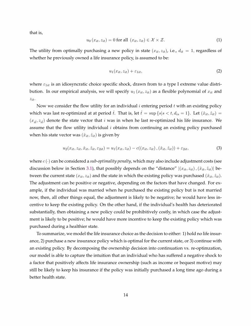
that is,
u0 (xit, zit) = 0 for all (xit, zit) ∈ X × Z. (1)
The utility from optimally purchasing a new policy in state (xit, zit), i.e., dit = 1, regardless of
whether he previously owned a life insurance policy, is assumed to be:
u1(xit, zit) + "1it, (2)
where "1it is an idiosyncratic choice specific shock, drawn from to a type I extreme value distri-
bution. In our empirical analysis, we will specify u1 (xit, zit) as a flexible polynomial of xit and
zit.
Now we consider the flow utility for an individual i entering period t with an existing policy
which was last re-optimized at at period t. That is, let t = sup {s∣s < t, dis = 1}. Let (xit, zit) =
(xit, zit) denote the state vector that i was in when he last re-optimized his life insurance. We
assume that the flow utility individual i obtains from continuing an existing policy purchased
when his state vector was (xit, zit) is given by
u2(xit, zit, xit, zit, "2it) = u1(xit, zit)− c((xit, zit) , (xit, zit)) + "2it, (3)
where c (⋅) can be considered a sub-optimality penalty, which may also include adjustment costs (see
discussion below in Section 3.1), that possibly depends on the “distance” ∣(xit, zit) , (xit, zit)∣ be-
tween the current state (xit, zit) and the state in which the existing policy was purchased (xit, zit).
The adjustment can be positive or negative, depending on the factors that have changed. For ex-
ample, if the individual was married when he purchased the existing policy but is not married
now, then, all other things equal, the adjustment is likely to be negative; he would have less in-
centive to keep the existing policy. On the other hand, if the individual’s health has deteriorated
substantially, then obtaining a new policy could be prohibitively costly, in which case the adjust-
ment is likely to be positive; he would have more incentive to keep the existing policy which was
purchased during a healthier state.
To summarize, we model the life insurance choice as the decision to either: 1) hold no life insur-
ance, 2) purchase a new insurance policy which is optimal for the current state, or 3) continue with
an existing policy. By decomposing the ownership decision into continuation vs. re-optimzation,
our model is able to capture the intuition that an individual who has suffered a negative shock to
a factor that positively affects life insurance ownership (such as income or bequest motive) may
still be likely to keep his insurance if the policy was initially purchased a long time ago during a
better health state.
14

Moreover, the decomposition of the ownership decision allows us to examine two separate
motives for lapsation: lapsation because the individual no longer needs any life insurance, and
lapsation because the policyholder’s personal situation, i.e. (xit, zit) , has changed such that new
coverage terms are required.
Parametric Assumptions on u1 and c Functions. In our empirical implementation of the model,
we let the observed state vector xit include age, log household income, sum of the number of
health conditions and marital status, and we let the unobserved state vector zit include z1it, z2itand z3it which respectively represent the unobserved components of income, health and bequest
motives.8 In Section 6 below, we will describe how we anchor these unobservables to their in-
tended interpretations and how we use sequential Monte Carlo method to simulate their posterior
distributions.
The primitives of our model are thus given by the utility function of optimally purchasing life
insurance u1, and the sub-optimality adjustment function c. Our specification for u1 (xit, zit) in
our empirical analysis is given by
u1(xit, zit) = �0 + �1AGEit + �2 (LOGINCOMEit + z1it)
+�3 (CONDITIONSit + z2it) + �4 (MARRIEDit + z3it) , (4)
and our specification for c(∣(xit, zit) , (xit, zit)∣) is:
c((xit, zit) , (xit, zit)) = �5 + �6(AGEit − ˆAGEit) + �7(AGEit − AGEit)2
+�8
(LOGINCOMEit + z1it − ˆLOGINCOMEit − z1it
)+ �9
(LOGINCOMEit + z1it − ˆLOGINCOMEit − z1it
)2+�10
(CONDITIONSit + z2it − ˆCONDITIONSit − z2it
)+ �11
(CONDITIONSit + z2it − ˆCONDITIONSit − z2it
)2+�12
∣∣∣MARRIEDit + z3it − ˆMARRIEDit − z3it∣∣∣ . (5)
Transitions of the State Variables. The state variables which the an individual must keep track
of depend on whether the individual is currently a policyholder. If he currently does not own a
policy, his state variable is simply his current state vector (xit, zit) ; if he currently owns a policy,
then his state variables include both his current state vector (xit, zit) and the state vector (xit, zit) at
8We do not include information regarding children also as potentially determinants of bequest motive for the fol-lowing reasons. If we include the “number of children” as one of the state variables, there is pratically no variationin our data set due to the ages of the individuals in our sample. Thus the effect of the variable “number of children”will be soaked into the constant term. However, if we include “age of the youngest child” or “number of dependentchildren” (i.e. children below age 18), we would have to include the ages of all children as part of the state variables,which significantly increases the dimensionality of our problem and make it untractible computationally.
15

which he purchased the policy he currently owns.
In our empirical analysis, we assume that the current state vectors (xit, zit) evolve exogenously
(i.e., not affected by the individual’s decision) according to a joint distribution given by
(xit+1, zit+1) ∼ f (xit+1, zit+1∣xit, zit) .
In particular, for the observed state vector xit, which includes age, log household income, sum of
the number of health conditions and marital status, we estimate their evolution directly from the
data. For the unobserved state vector zit, we will use sequential Monte Carlo methods to simulate
its evolution (see Section 6.2 below for details).
The evolution of the state vector (xit, zit) is endogenous, and it is given as follows. If the
individual does not own life insurance at period t, which we denote by setting (xit, zit) = ∅, then
(xit+1, zit+1)∣ (xit, zit) = ∅ =
⎧⎨⎩ (xit, zit) if dit = 1
∅ if dit = 0(6)
where ∅ denotes that the individual remains with no life insurance.
If the individual owns life insurance at period t purchased at state (xit, zit) , then
(xit+1, zit+1)∣ (xit, zit) ∕= ∅ =
⎧⎨⎩∅ if dit = 0
(xit, zit) if dit = 1
(xit, zit) if dit = 2.
(7)
3.1 Discussion
Dynamic Discrete Choice Model without the Knowledge of the Choice and Choice Set. As we
mentioned in Section 2, we do not have complete information about the exact life insurance poli-
cies owned by the individuals, and for those whose life insurance policy we do know about, we
do not know the choice set from which they choose. However, we do know whether an individual
has re-optimized his life insurance policy holdings (i.e., purchase a new life insurance policy, or
changed the amount of his existing coverage), or has dropped coverage etc.
The data restrictions we face are fairly typically for many applications.9 For example, in the
9McFadden (1978) and Fox (2007) studied problems where the researcher only observes the choices of decision-makers from a subset of choices. McFadden (1978) showed that in a class of discrete-choice models where choice specificerror terms have a block additive generalized extreme value (GEV) distributions, the standard maximum likelihoodestimator remains consistent. Fox (2007) proposed using semiparametric multinomial maximum-score estimator whenestimation uses data on a subset of the choices available to agents in the data-generating process, thus relaxing the
16
study of housing market, it is possible that all we observe is whether a family moved to a new
house, remained in the same house, or decided to rent; but we may not observe the characteristics
(including purchase price) of the new house the family moved into, or the characteristics of the
house/apartment the family rented.
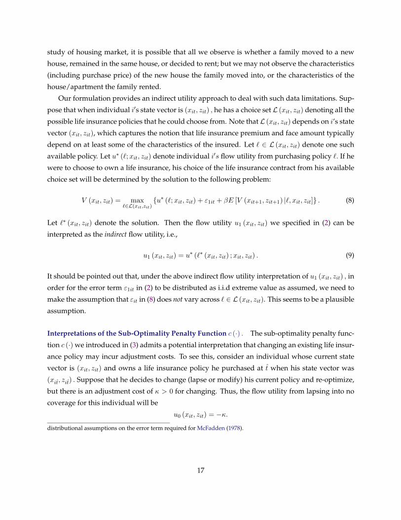
Our formulation provides an indirect utility approach to deal with such data limitations. Sup-
pose that when individual i′s state vector is (xit, zit) , he has a choice set ℒ (xit, zit) denoting all the
possible life insurance policies that he could choose from. Note that ℒ (xit, zit) depends on i’s state
vector (xit, zit), which captures the notion that life insurance premium and face amount typically
depend on at least some of the characteristics of the insured. Let ℓ ∈ ℒ (xit, zit) denote one such
available policy. Let u∗ (ℓ;xit, zit) denote individual i′s flow utility from purchasing policy ℓ. If he
were to choose to own a life insurance, his choice of the life insurance contract from his available
choice set will be determined by the solution to the following problem:
V (xit, zit) = maxℓ∈ℒ(xit,zit)
{u∗ (ℓ;xit, zit) + "1it + �E [V (xit+1, zit+1) ∣ℓ, xit, zit]} . (8)
Let ℓ∗ (xit, zit) denote the solution. Then the flow utility u1 (xit, zit) we specified in (2) can be
interpreted as the indirect flow utility, i.e.,
u1 (xit, zit) = u∗ (ℓ∗ (xit, zit) ;xit, zit) . (9)
It should be pointed out that, under the above indirect flow utility interpretation of u1 (xit, zit) , in
order for the error term "1it in (2) to be distributed as i.i.d extreme value as assumed, we need to
make the assumption that "it in (8) does not vary across ℓ ∈ ℒ (xit, zit). This seems to be a plausible
assumption.
Interpretations of the Sub-Optimality Penalty Function c (⋅) . The sub-optimality penalty func-
tion c (⋅) we introduced in (3) admits a potential interpretation that changing an existing life insur-
ance policy may incur adjustment costs. To see this, consider an individual whose current state
vector is (xit, zit) and owns a life insurance policy he purchased at t when his state vector was
(xit, zit) . Suppose that he decides to change (lapse or modify) his current policy and re-optimize,
but there is an adjustment cost of � > 0 for changing. Thus, the flow utility from lapsing into no
coverage for this individual will be
u0 (xit, zit) = −�.
distributional assumptions on the error term required for McFadden (1978).
17

The flow utility from re-optimizing, using the notation from (9), will be
u1 (xit, zit)− � = u∗ (ℓ∗ (xit, zit) ;xit, zit)− �.
And the flow utility from keeping the existing policy is
u2(xit, zit, xit, zit) = u∗ (ℓ∗ (xit, zit) ;xit, zit) = u∗ (ℓ∗ (xit, zit) ;xit, zit)
−
sub-optimality penalty︷ ︸︸ ︷[u∗ (ℓ∗ (xit, zit) ;xit, zit)− u∗ (ℓ∗ (xit, zit) ;xit, zit)]. (10)
where we used the notation ℓ∗ (xit, zit) to denote the optimal policy for state vector (xit, zit) .
Note that the term [u∗ (ℓ∗ (xit, zit) ;xit, zit)− u∗ (ℓ∗ (xit, zit) ;xit, zit)] indeed measures the utility
loss from holding a policy ℓ∗ (xit, zit) that was optimal for state vector (xit, zit) , but sub-optimal
when state vector is (xit, zit) .
If we were to normalize the flow utility from not owning life insurance u0 (xit, zit) = 0, we
essentially have
c (xit, zit;xit, zit) = [u∗ (ℓ∗ (xit, zit) ;xit, zit)− u∗ (ℓ∗ (xit, zit) ;xit, zit)]− �.
That is, our sub-optimality penalty c (⋅) indeed incorporates the adjustment cost � as a compo-
nent. It should be clear from the above discussion that the adjust cost � could easily be made a
function of both (xit, zit) and (xit, zit) . We will not be able to separate the sub-optimality penalty
[u∗ (ℓ∗ (xit, zit) ;xit, zit)− u∗ (ℓ∗ (xit, zit) ;xit, zit)] from � (xit, zit;xit, zit) .
Given the presence of adjust cost �, we would expect that an existing policyholders will hold
on to his policy until the sub-optimality penalty [u∗ (ℓ∗ (xit, zit) ;xit, zit)− u∗ (ℓ∗ (xit, zit) ;xit, zit)]
exceeds the adjustment cost �, if we ignore decisions driven by i.i.d preference shocks "1it and "2it.
Limitations of the “Indirect Flow Utility” Approach. While the “indirect flow utility” approach
we adopted in this paper to deal with the lack of information regarding individuals’ actual choices
of life insurance policies and their relevant choice set is useful for our purpose of understanding
why policyholders lapse their coverage (as we will demonstrate later), it has a major limitation.
The indirect flow utilities u1 (xit, zit) and u2(xit, zit, xit, zit) defined in (9) and (10) respectively, are
derived only under the existing life insurance market structure. As a result, the estimated indirect
flow utility functions are not primitives that are invariant to counterfactual policy changes that
may affect the equilibrium of the life insurance market. Of course, this limitation is also present in
other dynamic discrete choice models where the flow utility functions can have the interpretation
18
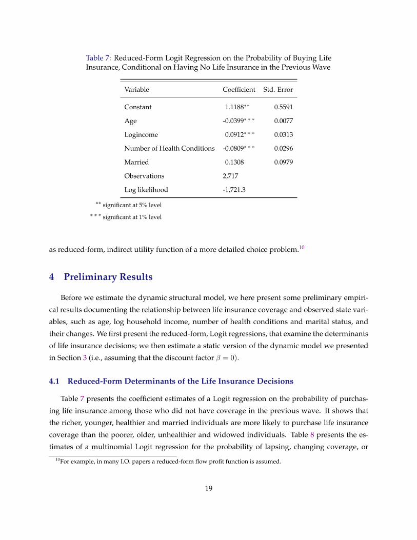
Table 7: Reduced-Form Logit Regression on the Probability of Buying LifeInsurance, Conditional on Having No Life Insurance in the Previous Wave
Variable Coefficient Std. Error
Constant 1.1188∗∗ 0.5591
Age -0.0399∗ ∗ ∗ 0.0077
Logincome 0.0912∗ ∗ ∗ 0.0313
Number of Health Conditions -0.0809∗ ∗ ∗ 0.0296
Married 0.1308 0.0979
Observations 2,717
Log likelihood -1,721.3
∗∗ significant at 5% level∗ ∗ ∗ significant at 1% level
as reduced-form, indirect utility function of a more detailed choice problem.10
4 Preliminary Results
Before we estimate the dynamic structural model, we here present some preliminary empiri-
cal results documenting the relationship between life insurance coverage and observed state vari-
ables, such as age, log household income, number of health conditions and marital status, and
their changes. We first present the reduced-form, Logit regressions, that examine the determinants
of life insurance decisions; we then estimate a static version of the dynamic model we presented
in Section 3 (i.e., assuming that the discount factor � = 0).
4.1 Reduced-Form Determinants of the Life Insurance Decisions
Table 7 presents the coefficient estimates of a Logit regression on the probability of purchas-
ing life insurance among those who did not have coverage in the previous wave. It shows that
the richer, younger, healthier and married individuals are more likely to purchase life insurance
coverage than the poorer, older, unhealthier and widowed individuals. Table 8 presents the es-
timates of a multinomial Logit regression for the probability of lapsing, changing coverage, or
10For example, in many I.O. papers a reduced-form flow profit function is assumed.
19
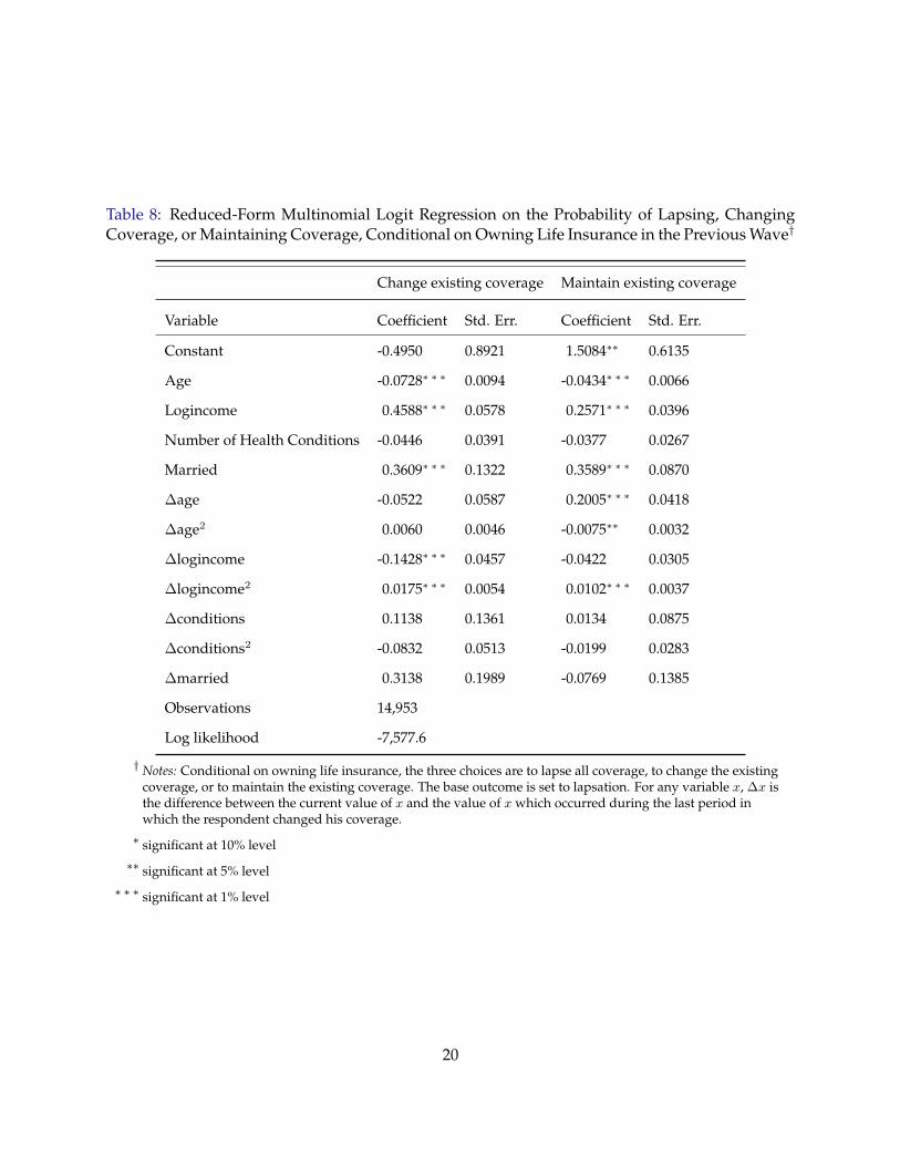
Table 8: Reduced-Form Multinomial Logit Regression on the Probability of Lapsing, ChangingCoverage, or Maintaining Coverage, Conditional on Owning Life Insurance in the Previous Wave†
Change existing coverage Maintain existing coverage
Variable Coefficient Std. Err. Coefficient Std. Err.
Constant -0.4950 0.8921 1.5084∗∗ 0.6135
Age -0.0728∗ ∗ ∗ 0.0094 -0.0434∗ ∗ ∗ 0.0066
Logincome 0.4588∗ ∗ ∗ 0.0578 0.2571∗ ∗ ∗ 0.0396
Number of Health Conditions -0.0446 0.0391 -0.0377 0.0267
Married 0.3609∗ ∗ ∗ 0.1322 0.3589∗ ∗ ∗ 0.0870
Δage -0.0522 0.0587 0.2005∗ ∗ ∗ 0.0418
Δage2 0.0060 0.0046 -0.0075∗∗ 0.0032
Δlogincome -0.1428∗ ∗ ∗ 0.0457 -0.0422 0.0305
Δlogincome2 0.0175∗ ∗ ∗ 0.0054 0.0102∗ ∗ ∗ 0.0037
Δconditions 0.1138 0.1361 0.0134 0.0875
Δconditions2 -0.0832 0.0513 -0.0199 0.0283
Δmarried 0.3138 0.1989 -0.0769 0.1385
Observations 14,953
Log likelihood -7,577.6
† Notes: Conditional on owning life insurance, the three choices are to lapse all coverage, to change the existingcoverage, or to maintain the existing coverage. The base outcome is set to lapsation. For any variable x, Δx isthe difference between the current value of x and the value of x which occurred during the last period inwhich the respondent changed his coverage.∗ significant at 10% level∗∗ significant at 5% level∗ ∗ ∗ significant at 1% level
20
maintaining the previous coverage. The omitted category is lapsing all coverage. The estimates
show that richer individuals are more likely to either maintain the current coverage or changing
existing coverage than to lapse all coverage; individuals who experienced negative income shocks
are more likely to lapse all coverages; individuals who are either divorced or widowed are more
likely to lapse all coverages; finally, individuals who have experienced an increase in the num-
ber of health conditions are somewhat more likely to lapse all coverage, though the effect is not
statistically significant.
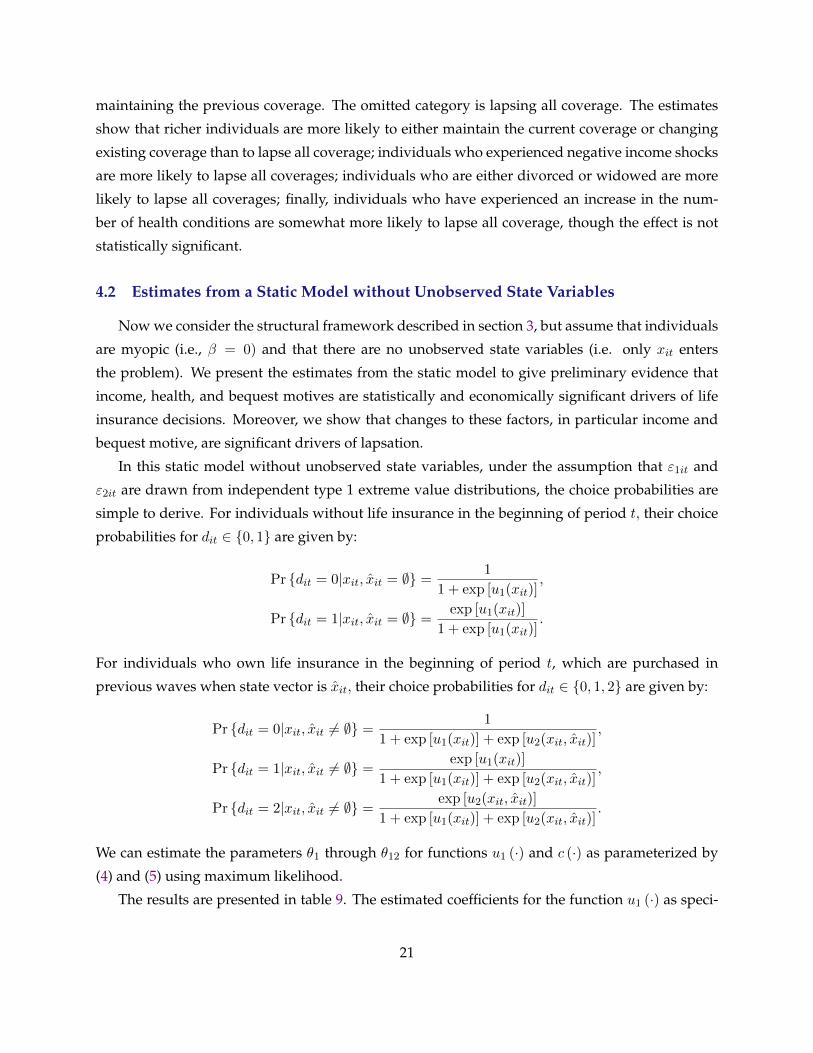
4.2 Estimates from a Static Model without Unobserved State Variables
Now we consider the structural framework described in section 3, but assume that individuals
are myopic (i.e., � = 0) and that there are no unobserved state variables (i.e. only xit enters
the problem). We present the estimates from the static model to give preliminary evidence that
income, health, and bequest motives are statistically and economically significant drivers of life
insurance decisions. Moreover, we show that changes to these factors, in particular income and
bequest motive, are significant drivers of lapsation.
In this static model without unobserved state variables, under the assumption that "1it and
"2it are drawn from independent type 1 extreme value distributions, the choice probabilities are
simple to derive. For individuals without life insurance in the beginning of period t, their choice
probabilities for dit ∈ {0, 1} are given by:
Pr {dit = 0∣xit, xit = ∅} =1
1 + exp [u1(xit)],
Pr {dit = 1∣xit, xit = ∅} =exp [u1(xit)]
1 + exp [u1(xit)].
For individuals who own life insurance in the beginning of period t, which are purchased in
previous waves when state vector is xit, their choice probabilities for dit ∈ {0, 1, 2} are given by:
Pr {dit = 0∣xit, xit ∕= ∅} =1
1 + exp [u1(xit)] + exp [u2(xit, xit)],
Pr {dit = 1∣xit, xit ∕= ∅} =exp [u1(xit)]
1 + exp [u1(xit)] + exp [u2(xit, xit)],
Pr {dit = 2∣xit, xit ∕= ∅} =exp [u2(xit, xit)]
1 + exp [u1(xit)] + exp [u2(xit, xit)].
We can estimate the parameters �1 through �12 for functions u1 (⋅) and c (⋅) as parameterized by
(4) and (5) using maximum likelihood.
The results are presented in table 9. The estimated coefficients for the function u1 (⋅) as speci-
21

Table 9: Estimation Results from the Static Discrete Choice Model
Estimate Std. Error
Panel A: Coefficients for u1(xit)
Constant 0.5905∗ ∗ ∗ 0.1167
Age -0.0448∗ ∗ ∗ 0.0013
Logincome 0.1784∗ ∗ ∗ 0.0077
Conditions -0.0710∗ ∗ ∗ 0.0055
Married 0.2766∗ ∗ ∗ 0.0198
Panel B: Coefficients for c(xit, xit)
Constant -1.7909∗ ∗ ∗ 0.0279
Δage -0.2320∗ ∗ ∗ 0.0100
Δage2 0.0099∗ ∗ ∗ 0.0007
Δlogincome 0.0090 0.0066
Δlogincome2 -0.0049∗ ∗ ∗ 0.0009
Δconditions -0.0202 0.0145
Δconditions2 -0.0024 0.0042
Δmarried 0.2094∗ ∗ ∗ 0.0334
Log likelihood -9,356.48
† Notes: Conditional on owning life insurance, the three choices are to lapse all coverage, to change the existingcoverage, or to maintain the existing coverage. The base outcome is set to lapsation. For any variable x, Δx isthe difference between the current value of x and x, which is the value of x at the time when the respondentchanged his coverage.
∗ ∗ ∗ significant at 1% level
22
fied in (4) indicate that married and higher-income individuals have more to gain from optimally
purchasing new insurance, whereas older and less healthy individuals have less to gain. This is
consistent with the interpretation that the cost of re-optimizing one’s life insurance increases when
one gets older and has poorer health, whereas marriage is a bequest factor that leads to the pur-
chase of life insurance; and individuals with higher incomes are also more likely to purchase life
insurance, partly because higher income makes any given amount of coverage more affordable
and partly because individuals with higher incomes would like to leave more bequests to their
dependents.
The large, negative constant term in the sub-optimality adjustment function c (⋅) indicates that
policyholders are likely to keep their existing policies even if the state of the world changed sig-
nificantly from when they last re-optimized. This is consistent with an interpretation of high
adjustment costs. This could be driven either by search costs or the existence whole-life policies
which build up a cash value which is uncontrolled for in our model.
The negative coefficients on ΔAGE≡AGEt− AGEt and ΔCONDITIONS tell us that as the policy-
holder gets older, or becomes less healthy, it becomes more costly to re-optimize, though the effect
of ΔCONDITIONS is not statistically significant. Moreover, the negative effect of ΔAGE on c (⋅) is
nonlinear, though in reasonable ranges of ΔAGE the positive coefficient estimate on (ΔAGE)2 will
not over-ride the overall negative effect of ΔAGE on c (⋅) . These estimates are again consistent
with the interpretation of age and health as cost factors related to the purchase of new policies.
The positive coefficient estimate on Δ logINCOME indicate that policyholders are more likely to
stay with their existing policy when income has declined, but more likely to re-optimize when
income has risen (the quadratic term reverses the sign of the linear term in only less than 1% of
our observations). Finally, the coefficient on Δmarried indicates that a policyholder whose marital
status has changed is more likely to re-optimize than to continue an existing policy.
It will be useful now to look at the quantitative predictions of our model. Let us first look at the
own or not own decision margin for existing policyholders. For the average married respondent in
our data set in 1996, a 10% drop in household income, everything else equal, increases the chance
of lapsing to no life insurance by about 1.7%. If this same individual instead goes from married
to not married, he is 50% more likely to drop all insurance coverage. A 10% drop in household
income is far more likely than the loss of a marriage, however, so let us instead ask what happens
if income drops by 85%, which is about as likely in our data as losing the marriage. Such a drop
in income increases the likelihood of lapsing to nothing by about 34%.
Now let us consider the “re-optimize” vs. “continue the existing policy” decision margin. For
the average individual in 1996, if the current income is 10% higher than the income at the time
of last re-optimization, the likelihood of re-optimizing increases by only 0.21%. Even if current
23

income is double the income at the time of last re-optimization, the likelihood of re-optimizing
increases by only 1.24%. If, on the other hand, the respondent was married when he last re-
optimized but is not married now, his chances of re-optimizing increase by 15%.
To summarize, we have shown that lapsation works over two channels: lapsation due to no
longer needing life insurance, and lapsation due to re-optimization of an existing policy. We have
also shown that changes to income and marital status are statistically significant drivers in both
these channels. Changes to income and marital status are shown to be important drivers of lap-
sation along the “own a policy” vs. “not own a policy” margin, but only marital status seems to
have an economically significant effect along the “re-optimize” vs. “continue the existing policy”
margin. We have also shown that re-optimization costs are high, so that many individuals prefer
to keep existing policies even if their current state is far from their original state.
While informative, the static model is not equipped to answer the main question of our interest,
how lapsation patterns would change if all variability to marital status or income were removed
counterfactually. The reason is that a static model does not take into account the change in a
policyholder’s expectations that accompanies a change in the transition processes. For example,
suppose that we make income much more volatile than it is. A reduced form model would predict
a lot more lapsation, and also a lot more purchasing. But in a dynamic model, consumers correctly
anticipate the riskiness of income, and will not respond as much to temporary shocks. To answer
the question satisfactorily, we will now reintroduce dynamics into our framework in the next
section.
5 Estimates from a Dynamic Discrete Choice Model Without
Unobservable State Variables
In this section, we present our estimation and simulation results for the dynamic structural
model of life insurance decisions presented in Section 3. However, in order to illustrate the im-
portance of unobserved state variables in the life insurance decisions (which we turn to in the
next section), we deliberately do not include any unobserved state variables zit in this section.
The estimation and simulation results for a dynamic discrete choice model with unobserved state
variables are presented in Section 6.
As described in Section (3) the flow utilities are given by equations (1)-(3). Since we only
include observed state variables in this section, we will for simplicity denote the transition distri-
butions of the state variables xit by P (xit∣xit−1). Since xit are observable, we estimate P (xit∣xit−1)separately and then take it as given. As we mentioned in Section 3, we assume that the evolution
of the state variables xit does not depend on the life insurance choices analyzed in this model.
24
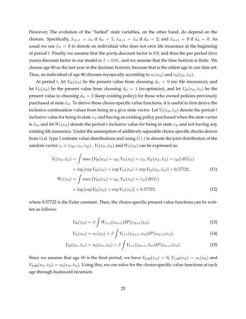
However, The evolution of the “hatted” state variables, on the other hand, do depend on the
choices. Specifically, xit+1 = xit if dit = 1; xit+1 = xit if dit = 2; and xit+1 = ∅ if dit = 0. As
usual we use xit = ∅ to denote an individual who does not own life insurance at the beginning
of period t. Finally, we assume that the yearly discount factor is 0.9, and thus the per period (two
years) discount factor in our model is � = 0.81, and we assume that the time horizon is finite. We
choose age 80 as the last year in the decision horizon, because that is the oldest age in our data set.
Thus, an individual of age 80 chooses myopically according to u1(xit) and u2(xit, xit).
At period t, let V0t(xit) be the present value from choosing dit = 0 (no life insurance); and
let V1t(xit) be the present value from choosing dit = 1 (re-optimize), and let V2t(xit, xit) be the
present value to choosing dit = 2 (keep existing policy) for those who owned policies previously
purchased at state xit. To derive these choice-specific value functions, it is useful to first derive the
inclusive continuation values from being in a give state vector. Let Vt(xit, xit) denote the period-t
inclusive value for being in state xit and having an existing policy purchased when the state vector
is xit, and let Wt(xit) denote the period-t inclusive value for being in state xit and not having any
existing life insurance. Under the assumption of additively separable choice specific shocks drawn
from i.i.d. type 1 extreme value distributions and using G (⋅) to denote the joint distribution of the
random vector "t ≡ ("0t, "1t, "2t) , Vt(xit, xit) and Wt(xit) can be expressed as:
Vt(xit, xit) =
∫max {V0t(xit) + "0t, V1t(xit) + "1t, V2t(xit, xit) + "2t} dG("t)
= log [expV0t(xit) + expV1t(xit) + expV2t(xit, xit)] + 0.57722, (11)
Wt(xit) =
∫max {V0t(xit) + "0t, V1t(xit) + "1t} dG(")
= log [expV0t(xit) + expV1t(xit)] + 0.57722, (12)
where 0.57722 is the Euler constant. Then, the choice-specific present value functions can be writ-
ten as follows:
V0t(xit) = �
∫Wt+1(xit+1)dP (xit+1∣xit), (13)
V1t(xit) = u1(xit) + �
∫Vt+1(xit+1, xit)dP (xit+1∣xit), (14)
V2t(xit, xit) = u2(xit, xit) + �
∫Vt+1(xit+1, xit)dP (xit+1∣xit). (15)
Since we assume that age 80 is the final period, we have V0,80(xit) = 0, V1,80(xit) = u1(xit) and
V2,80(xit, xit) = u2(xit, xit). Using this, we can solve for the choice-specific value functions at each
age through backward recursion.
25
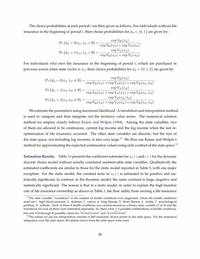
The choice probabilities at each period t are then given as follows. For individuals without life
insurance in the beginning of period t, their choice probabilities for dit ∈ {0, 1} are given by:
Pr {dit = 0∣xit, xit = ∅} =expV0t(xit)
expV0t(xit) + expV1t(xit),
Pr {dit = 1∣xit, xit = ∅} =expV1t(xit)
expV0t(xit) + expV1t(xit).
For individuals who own life insurance in the beginning of period t, which are purchased in
previous waves when state vector is xit, their choice probabilities for dit ∈ {0, 1, 2} are given by:
Pr {dit = 0∣xit, xit ∕= ∅} =expV0t(xit)
expV0t(xit) + expV1t(xit) + expV2t(xit, xit),
Pr {dit = 1∣xit, xit ∕= ∅} =expV1t(xit)
expV0t(xit) + expV1t(xit) + expV2t(xit, xit),
Pr {dit = 2∣xit, xit ∕= ∅} =expV2t(xit, xit)
expV0t(xit) + expV1t(xit) + expV2t(xit, xit).
We estimate the parameters using maximum likelihood. A simulation and interpolation method
is used to compute and then integrate out the inclusive value terms. The numerical solution
method we employ closely follows Keane and Wolpin (1994). Among the state variables, two
of them are allowed to be continuous, current log income and the log income when the last re-
optimization of life insurance occurred. The other state variables are discrete, but the size of
the state space, not including log incomes, is also very large.11 We thus use Keane and Wolpin’s
method for approximating the expected continuation values using only a subset of the state space.12
Estimation Results. Table 10 presents the coefficient estimates for u1 (⋅) and c (⋅) for the dynamic
discrete choice model without serially correlated unobservable state variables. Qualitatively the
estimated coefficients are similar to those for the static model reported in Table 9, with one major
exception. For the static model, the constant term in u1 (⋅) is estimated to be positive and sta-
tistically significant; in contrast, in the dynamic model, the same constant is large, negative and
statistically significant. The reason is that in a static model, in order to explain the high baseline
rate of life insurance ownership as shown in Table 3, the flow utility from owning a life insurance
11The state variable ”conditions” is the number of health conditions ever diagnosed, where the health conditionsused are:1. high blood pressure; 2. diabetes; 3. cancer; 4. lung disease; 5. heart disease; 6. stroke; 7. psychologicalproblem; 8. arthritis. Each of these 8 health conditions was carried around as a binary state variable (1 or 0) and thetransitions for each of these were estimated separately. So, there were 2ˆ8 possible combinations of health conditions,but only 9 (0 through 8) possible values for ”CONDITIONS” and ” ˆCONDITIONS”.
12The subset we use for interpolation consists of 400 randomly drawn points in the state space. For the numericalintegration over the state space, 40 random draws from the state space were used.
26
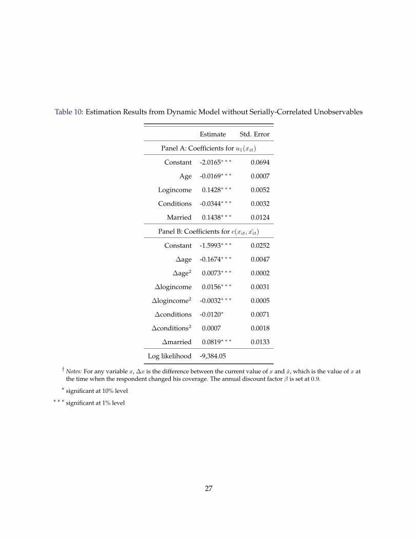
Table 10: Estimation Results from Dynamic Model without Serially-Correlated Unobservables
Estimate Std. Error
Panel A: Coefficients for u1(xit)
Constant -2.0165∗ ∗ ∗ 0.0694
Age -0.0169∗ ∗ ∗ 0.0007
Logincome 0.1428∗ ∗ ∗ 0.0052
Conditions -0.0344∗ ∗ ∗ 0.0032
Married 0.1438∗ ∗ ∗ 0.0124
Panel B: Coefficients for c(xit, xit)
Constant -1.5993∗ ∗ ∗ 0.0252
Δage -0.1674∗ ∗ ∗ 0.0047
Δage2 0.0073∗ ∗ ∗ 0.0002
Δlogincome 0.0156∗ ∗ ∗ 0.0031
Δlogincome2 -0.0032∗ ∗ ∗ 0.0005
Δconditions -0.0120∗ 0.0071
Δconditions2 0.0007 0.0018
Δmarried 0.0819∗ ∗ ∗ 0.0133
Log likelihood -9,384.05
† Notes: For any variable x, Δx is the difference between the current value of x and x, which is the value of x atthe time when the respondent changed his coverage. The annual discount factor � is set at 0.9.∗ significant at 10% level
∗ ∗ ∗ significant at 1% level
27
must be high; in a dynamic model, owning life insurance could be attractive relative to not own-
ing life insurance if the continuation value of owning life insurance is sufficiently large. Thus in a
dynamic model, a positive constant in u1 (⋅) is not needed to fit the high life insurance ownership
rate observed in the data.
The large negative constant term estimated for c (⋅) still indicates high adjustment costs for
changing one’s life insurance policy (see the discussion in Section 3.1). In Panel B, same as the
estimates for the static model reported in Table 9, the negative coefficients on ΔAGE≡AGEt− AGEt
and ΔCONDITIONS tell us that as the policyholder gets older, or becomes less healthy, it becomes
more costly to re-optimize. Note that the negative coefficient on ΔCONDITIONS is now statistically
significant at 10% level. The finding that the less healthy policyholders are more likely to keep the
existing policy, or alternatively, the healthier policyholders are more likely to re-optimize or lapse,
is consistent with the predictions of adverse selection in lapsation decisions in Hendel and Lizzeri
(2003) and is consistent with the empirical findings of He (2010).
Model Fit. To assess the performance of the dynamic model without unobservable state vari-
ables, we report in Panel A of Table 11 the comparisons between the simulated model predictions
regarding aggregate choice probabilities by wave and those in the data. It shows that the dynamic
model without serially correlated unobservable state variables does a fairly good job at predicting
the aggregate distribution of choices, but there appears to be a dynamic effect which our model
is not capturing. Specifically, the actual data exhibits that, in the aggregate, there is an increasing
likelihood over time of holding no life insurance, and a decreasing likelihood over time of keeping
an existing policy. These two patterns do not appear to be fully captured by our model.
In Panel B of Table 11, we report the comparison between the simulated model predictions of
the cumulative outcomes for individuals who owned life insurance in 1994 by wave and those in
the data. In the actual data, the cumulative fraction of 1994 policyholders lapsing to no insurance
steadily increases over time, going from 4.55% in 1996 to 23.40% by 2006. The model simulation
is not able to replicate the initially low lapsation rates. The model also under-predicts by large
margin the cumulative fraction of the 1994 policyholders who kept their policies.13
Because the dynamic model without serially correlated unobservable state variables fails to
13In un-reported counterfactual simulations we find that elimination of marital shocks has a larger effect on lapsationpatterns than elimination of income shock. Elimination of marital shocks reduces the share of policies lapsing to noinsurance, as well as the share of policies which are re-optimized. Elimination of income shocks reduces the share ofpolicies lapsing to none, but increases the share of policies which are re-optimized. The increase in re-optimization isdue to the fact that income is generally going down for individuals of our age range.
However, our counterfactual simulations also show that elimination of either of these shocks has an economicallyinsignificant impact on the aggregate lapsation patterns. Most of the lapsation in our data seems to be driven byunobserved, idiosyncratic factors. This is not surprising given that marital status and income are not very volatile inour data.
28

Table 11: Model Fit for Dynamic Model without Serially Correlated Unobservable State Variables
Wave
1996 1998 2000 2002 2004 2006
Panel A: Aggregate Choice Probabilities by Wave
Actual Data
No life insurance coverage 0.1194 0.1427 0.1648 0.1896 0.1951 0.2138
Covered, but changed or bought new coverage 0.1495 0.1077 0.0963 0.0978 0.1126 0.0946
Covered, and kept existing coverage 0.7310 0.7496 0.7389 0.7127 0.6923 0.6916
Simulation using dynamic model without serially correlated unobservables
No life insurance coverage 0.1772 0.1714 0.1637 0.1639 0.1759 0.1985
Covered, but changed or bought new coverage 0.1410 0.1280 0.1134 0.1038 0.1005 0.1009
Covered, and kept existing coverage 0.6818 0.7006 0.7228 0.7323 0.7236 0.7006
Panel B: Cumulative Outcomes for 1994 Policyholders
Actual data
Lapsed to no life insurance 0.0455 0.0899 0.1358 0.1792 0.2095 0.2340
Changed coverage amount 0.0903 0.1472 0.1846 0.2080 0.2283 0.2489
Kept 1994 coverage 0.8642 0.7315 0.6138 0.5203 0.4491 0.3812
Policyholder died 0.0000 0.0313 0.0658 0.0924 0.1131 0.1358
Simulation using dynamic model without serially correlated unobservables
Lapsed to no life insurance 0.1048 0.1643 0.2059 0.2401 0.2734 0.3085
Changed coverage amount 0.0892 0.1375 0.1683 0.1911 0.2114 0.2307
Kept 1994 coverage 0.8060 0.6689 0.5671 0.4831 0.4101 0.3369
Policyholder died 0.0000 0.0293 0.0587 0.0857 0.1051 0.1239
29
match the dynamic persistence in both the aggregate choice probabilities and cumulative out-
comes, we suspect that some of these idiosyncratic factors may not be so idiosyncratic at all. In
particular, if there are serially correlated unobservables, such as unobserved components of be-
quest motive or liquidity shocks, then our model will fall short in explaining the empirical deter-
minants of lapsation. Indeed, our simulations seem to over-forecast lapsation due to no longer
needing life insurance and under-forecast lapsation due to re-optimization, indicating the pres-
ence of some persistent unobservable that positively influences the likelihood of needing life in-
surance. In the next section, we develop and estimate a model that explicitly takes into account
the presence of unobserved state variables.
6 Estimates from Dynamic Discrete Choice Model with Unobserved
State Variables
In this section we take the dynamic model presented in section 5 and add three unobserved
state variables: z1, z2 and z3. We are now fully back to the empirical framework we presented
earlier in Section 3.
6.1 Anchoring the Unobserved State Variables
In this specification, we would like to give the unobserved state variable z1 the interpretation
as an unobserved liquidity (or income) shock, and normalize its unit to the same as log income, and z2the interpretation as an unobserved health shock that is normalized to the units of health conditions,
and finally z3 the interpretation as an unobserved component of bequest motive that is normalized to
the units of marital status.
We assume that the initial distribution in 1994 (t = 0) for each of these unobserved variables is
degenerate and given by:14
z1i0 = �13ℎi0, (16)
z2i0 = �14ℎi0, (17)
z3i0 = �15ℎi0, (18)
where ℎi0 is an indicator dummy for whether the individual reported owning life insurance in
1994. In order to anchor z1, z2 and z3 to have the desired interpretation given above, we restrict in
14We could allow the distributions of z0 to depend on ℎi0 in that the means of z0 is higher for those with ℎi0 = 1.The assumption that the initial distribution of the unobservable state variables z0 is degenerate is for computationalsimplicity.
30

our estimation that the coefficients �13, �14 and �15 to be strictly positive, thus ensuring that those
with life insurance in the initial period also had higher values for the unobservable. For example,
because income is a positive factor for life insurance ownership, we restrict the sign of �13 to be
positive, so that individuals who owned life insurance in the initial period also have higher z1.
This anchors the interpretation of z1 as an unobserved component of income.
The second channel that anchors the unobserved state variables to having the desired inter-
pretation is incorporated in our specifications for u1 (⋅) and c (⋅) , as formulated in (4) and (5).
Note that we restricted z1i to entering both u1 (⋅) and c (⋅) in the same way as LOGINCOME, z2ithe same way as CONDITIONS, and z3i the same way as MARRIED. These restrictions, together
with the sequential Monte Carlo method (described in the next section below) we use to simulate
the distributions of zt ≡ (z1t, z2t, z3t) , ensures that the unobserved variables zt have the desired
interpretations.
If we know the distributions of the unobservable state vectors (zt, zt) , solving this model is
done no differently from that in section 5. Given a vector of parameters � = (�0, ..., �21) , we can
compute the value functions at each age through backward recursion. The difficulty of handling
unobserved state variables comes during estimation, because we have to integrate over the unob-
servables when computing the likelihood. We now turn our attention to this problem.
6.2 Using Sequential Monte Carlo Method to Simulate the Distributions of theUnobserved State Variables
We use Sequential Monte Carlo (SMC) method to simulate the distributions of the unobserv-
able state vectors.15 SMC is a set of simulation-based methods which provides a convenient and at-
tractive approach to computing the posterior distributions of involving non-Gaussian, non-linear,
and high dimensional random variables.16 A thorough discussion of the method, from both the
theoretical and the practical perspectives, is available in Doucet, de Freitas and Gordon (2001). The
SMC method has been widely used in fields such as speech recognition, biology, and physics, etc.
Despite the obvious potential importance of serially correlated unobservable state variables, there
are only few applications of SMC in the economics literature. Fernandez-Villaverde and Rubio-
Ramirez (2007) used SMC for estimating macroeconomic dynamic stochastic general equilibrium
models with serially correlated unobservable state variables using a likelihood approach. Blevins
(2008) proposed the use of SMC to allow for serially correlated unobservable state variables in
estimating dynamic single agent models and dynamic games. Hong, Gallant and Khwaja (2008)15SMC algorithms are also called bootstrap filters, particle filters, and sequential importance samplers with resam-
pling.16SMC for non-linear, non-Gaussian models is the analog of Kalman filter for linear, Gaussian models. Gordon,
Salmond and Smith (1993) is the seminal paper that proposed this algorithm, which they refer to as the bootstrap filter.
31

also discusses the method in an application to the pharmaceuticals industry. All of the papers
allow for a single serially correlated unobservable state variable. In our application, as we have
mentioned above, we believe that there might be important serially unobservable components for
each of the three potential sources of lapsation, shocks to income, health and bequest motives.
Now we provide a detailed discussion about the SMC. For a given individual, we observe the
sequence of choices {dt}Tt=0, observed state variables {xt, xt}Tt=0, and whether the individual had
life insurance in 1994 ℎ0. The data set is thus {dt, xt, xt, ℎ0}Tt=0 (we have dropped the i subscript
for convenience). Let p(d0:T ∣x0:T , x0:T , ℎ0) denote the conditional likelihood of the observed data.
We can write:
p(d0:T ∣x0:T , x0:T , ℎ0) = p(d0∣x0, x0, ℎ0)T∏t=1
p(dt∣dt−1, xt, xt) (19)
Because the initial distribution of z0 is degenerate and depends only on ℎ0, we can write:
p(d0∣x0, x0, ℎ0) = p(d0∣x0, x0, z0).
Assuming we have solved for the value functions in a first stage, we should be able to compute
p(d0∣x0, x0, z0).
Now, for each t > 0 we can write:
p(dt∣dt−1, xt, xt) =
∫p(dt∣dt−1, xt, xt, zt, zt)p(zt, zt∣dt−1)dztdzt. (20)
We know how to compute p(dt∣dt−1, xt, xt, zt, zt) for a given set of parameter values �. What we
need is a method to draw from p(zt, zt∣dt−1). Sequential Monte Carlo method can help us here.
It is a recursive algorithm that begins by drawing a swarm of particles approximating the
initial distribution of the hidden state. The initial swarm is then used to draw a swarm for the
next period, and this swarm is then filtered according to sequential importance weights.
The unobservables transition according to the following equations:
z1it = �16z1it−1 + �19�z1t, (21)
z2it = �17z2it−1 + �20�z2t, (22)
z3it = �18z3it−1 + �21�z3t, (23)
where �z1t, �z2t and �z3t are is an i.i.d. random variable with standard normal distribution N (0, 1).
The transition distribution of the observed state variables are given by P (xit∣xit−1) as in section
5.17
17Thus, we do not allow the transitions of the observed state variables to depend on the realization of the unobserved
32
The filtered particles are then used to draw another swarm for the next period, and so on.
In the following notation, we will absorb z into z and use z to denote any unobserved variable,
including the “hatted” z’s.
The method proceeds as follows:
0. Set t = 0, draw a swarm of particles{z(r)0
}R
r=1from the initial distribution p(z0). This distri-
bution must be parametrically assumed, with potentially unknown parameters. In our case
it is assumed to be degenerate as described by (16)-(18). Set t = 1.
1. For t > 0, use{z(r)t−1
}R
r=1to draw a new swarm
{z(r)t
}R
r=1from the distribution p(zt∣zt−1, dt−1).
This distribution is known because we have imposed a parametric specification on it. The
previous period’s choice, dt−1, is required because that determines how the “hatted” z’s
evolve. The swarm of particles {zt,r}Rr=0 now approximates the distribution p(zt∣dt−1).
2. For each r = 1, . . . R, computew(r)t = p(dt∣dt−1, xt, xt, zt,r). The vector
{w
(r)t
}R
r=1is known as
the vector of importance weights. We can now approximate the integral in (20) by 1R
∑Rr=1w
(r)t .
3. Draw a new swarm of particles{z(r)t
}R
r=1by drawing with replacement from
{z(r)t
}R
r=1. Use
the normalized importance weights as sampling probabilities.
4. Set t = t+ 1 and go to step 1.
Figure 1 presents a graphical representation of the SMC algorithm. In the graph, we assume
away for simplicity the unobservable state vectors carried from the last re-optimization period zt
for simplicity. The SMC starts at time t−1 with an un-weighted measure{z(r)t−1, R
−1},which pro-
vides an approximation of p (zt−1∣d1:t−2) . For each particle, we compute the importance weights
using the information about the actual choice dt−1 at time t − 1 with the weights given by the
model’s prediction of the likelihood p(dt−1∣z(r)t−1
)of observing dt−1 when the particle is z(r)t−1, prop-
erly re-normalized. This results in the weighted measure{z(r)t−1, w
(r)t−1
}, which yields an approx-
imation of p (zt−1∣d1:t−1) . Subsequently, the re-sampling with replacement (or the selection) step
selects only the fittest particles to obtain the un-weighted measure{z(r)t−1, R
−1}, , which is still an
approximation of p (zt−1∣d1:t−1) . Finally, the prediction step draws new varieties of particles from
the parametric process p (zt∣zt−1) , resulting in the measure{z(r)t , R−1
}, which is an approxima-
tion of p (zt∣d1:t−1) . The measures{z(r)t−1, R
−1}
and{z(r)t , R−1
}are the posterior distributions of
the unobservables we use in the numerical integration of the choice probabilities (20).
state variables.
33

u u u u u u u u u u
????
?
?
? ?
?
?
u z ~ z u z
e ee
eee
ee
e e
u u u u u u u u u u? ?
BBBN
����6?
JJJ ?
AAAU ? ?
�{z(r)t−1, R
−1}
Importance Sampling:p (dt−1∣zt−1)
�{z(r)t−1, w
(r)t−1
}
� Prediction: p (zt∣zt−1)
�{z(r)t , R−1
}
? ? ? ? ? ?�
�{z(r)t−1, R
−1}Selection
? ? ? ? ? ? ? ? ? ?
Figure 1: A Graphical Representation of the Sequential Monte Carlo Algorithm: Adapted fromDoucet, de Freitas and Gordon (2001, Chapter 1, p. 12)
At each iteration, we computed the per period probability of observing the data given by
equation (20) . Because this is done iteratively, starting from t = 0, we can eventually work our
way up to t = T and compute the entire likelihood given by (19). Repeating this process for each
individual for the data will give us the entire likelihood of the data. We can then estimate the
parameters via maximum likelihood.18
We use simulated maximum likelihood method to estimate the parameters of u1 (⋅) , c (⋅), the
initial values of z1, z2 and z3, as well as their AR(1) auto-correlation coefficients �14-�16 and vari-
ance terms �17-�19 as described in (21)-(23). We compute the standard errors using a bootstrap
procedure. In each iteration of the procedure, a new random seed is used to create a bootstrapped
sample of individuals from the original roster. The structural parameters are then re-estimated
using this bootstrapped sample. 50 bootstrapped samples were used. For each structural pa-
rameter, the standard error is calculated as the standard deviation of the estimates from the 5018We employed 64 particles in each swarm to integrate out the z’s when computing the conditional choice probabili-
ties. We use 40 articles when computing the expected future value term. One evaluation of the likelihood takes about2 minutes on an 8-core, 2.5GHz, 64 bit AMD computer while using all 8 CPUs, and the entire estimation routine tookabout 4 days when starting from an initial guess of all zeros.
34

bootstrapped samples.19
6.3 Estimation Results
Table 12 presents the estimation results. Panel A shows the estimated coefficients for u1 (xit, zit)
as specified in (4). The magnitudes of the estimated coefficients change from , but the signs of all
coefficients are consistent with, those for the model without serially correlated unobservables as
in Table 10.
Panel B presents the estimated coefficients for c ((xit, zit) , (xit, zit)) as specified in (5). There
are several important changes in the estimates for c (⋅) when unobservable state variables are in-
cluded. In contrast to the estimates in Table 10 for the model without serially correlated unobserv-
ables, now the changes in log income (the sum of observed and unobserved income components)
has a positive quadratic relationship with the cost function c (⋅). Also notice that coefficient es-
timate for LOGINCOME+z2 is positive in u1 (⋅) . These suggest that small or medium changes in
income is likely to lead to the existing policies being kept, but large negative in income will lead
to lapsation into no life insurance, and large positive changes in income will lead to re-optimizing
into a new life insurance. The implications from the estimates in Table 10 are exactly the opposite
and less plausible. Also, the positive estimates on the coefficients on both Δ (CONDITIONS + z2)
and Δ (CONDITIONS + z2)2 in c (⋅) and the negative coefficient estimate of CONDITIONS+z2 in
u1 (⋅) suggest that, again, small changes in health will lead to the keeping of the existing poli-
cies, however, large improvements in health conditions is likely to lead to lapsation into no life
insurance, and large deteriorations in health will lead to re-optimizing into a new coverage. Fi-
nally, the negative coefficient estimate on Δ (MARRIED + z3) in c (⋅) and the positive coefficient
estimate of MARRIED+z3 in u1 (⋅) suggest that a decrease in bequest motive will likely lead to lap-
sation into or stay with no life insurance, and an increase in bequest motive is likely to lead to the
purchase of new policy for individuals initially without coverage.
Panel C presents the estimates of the initial distributions of z1, z2 and z3 as a function of the
indicator of whether the individuals owned life insurance in 1994. These coefficients are restricted
to be positive as part of our strategies to anchor the interpretations of these unobservables. Panel
D presents the estimates of the coefficients of the autoregressive processes described in (21)-(23).
They suggest that the unobservable income and health shocks are mean reverting processes, how-
ever, the unobservable bequest motive shock is rather persistent.
19See Olsson and Ryden (2008) for a discussion about the asymptotic performance of approximate maximum likeli-hood estimators for state space models obtained via sequential Monte Carlo methods. It provides criteria for how toincrease the number of particles and the resolution of the grid in order to produce estimates that are consistent andasymptotically normal.
35
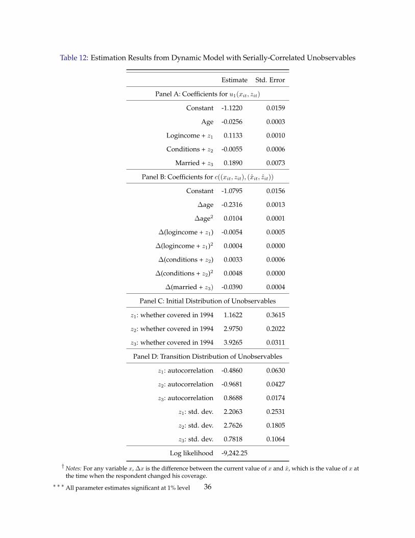
Table 12: Estimation Results from Dynamic Model with Serially-Correlated Unobservables
Estimate Std. Error
Panel A: Coefficients for u1(xit, zit)
Constant -1.1220 0.0159
Age -0.0256 0.0003
Logincome + z1 0.1133 0.0010
Conditions + z2 -0.0055 0.0006
Married + z3 0.1890 0.0073
Panel B: Coefficients for c((xit, zit), (xit, zit))
Constant -1.0795 0.0156
Δage -0.2316 0.0013
Δage2 0.0104 0.0001
Δ(logincome + z1) -0.0054 0.0005
Δ(logincome + z1)2 0.0004 0.0000
Δ(conditions + z2) 0.0033 0.0006
Δ(conditions + z2)2 0.0048 0.0000
Δ(married + z3) -0.0390 0.0004
Panel C: Initial Distribution of Unobservables
z1: whether covered in 1994 1.1622 0.3615
z2: whether covered in 1994 2.9750 0.2022
z3: whether covered in 1994 3.9265 0.0311
Panel D: Transition Distribution of Unobservables
z1: autocorrelation -0.4860 0.0630
z2: autocorrelation -0.9681 0.0427
z3: autocorrelation 0.8688 0.0174
z1: std. dev. 2.2063 0.2531
z2: std. dev. 2.7626 0.1805
z3: std. dev. 0.7818 0.1064
Log likelihood -9,242.25
† Notes: For any variable x, Δx is the difference between the current value of x and x, which is the value of x atthe time when the respondent changed his coverage.
∗ ∗ ∗ All parameter estimates significant at 1% level 36
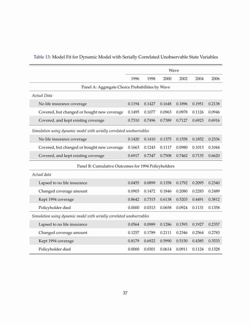
Table 13: Model Fit for Dynamic Model with Serially Correlated Unobservable State Variables
Wave
1996 1998 2000 2002 2004 2006
Panel A: Aggregate Choice Probabilities by Wave
Actual Data
No life insurance coverage 0.1194 0.1427 0.1648 0.1896 0.1951 0.2138
Covered, but changed or bought new coverage 0.1495 0.1077 0.0963 0.0978 0.1126 0.0946
Covered, and kept existing coverage 0.7310 0.7496 0.7389 0.7127 0.6923 0.6916
Simulation using dynamic model with serially correlated unobservables
No life insurance coverage 0.1420 0.1410 0.1375 0.1558 0.1852 0.2336
Covered, but changed or bought new coverage 0.1663 0.1243 0.1117 0.0980 0.1013 0.1044
Covered, and kept existing coverage 0.6917 0.7347 0.7508 0.7462 0.7135 0.6620
Panel B: Cumulative Outcomes for 1994 Policyholders
Actual data
Lapsed to no life insurance 0.0455 0.0899 0.1358 0.1792 0.2095 0.2340
Changed coverage amount 0.0903 0.1472 0.1846 0.2080 0.2283 0.2489
Kept 1994 coverage 0.8642 0.7315 0.6138 0.5203 0.4491 0.3812
Policyholder died 0.0000 0.0313 0.0658 0.0924 0.1131 0.1358
Simulation using dynamic model with serially correlated unobservables
Lapsed to no life insurance 0.0564 0.0989 0.1286 0.1593 0.1927 0.2357
Changed coverage amount 0.1257 0.1789 0.2111 0.2346 0.2564 0.2783
Kept 1994 coverage 0.8179 0.6922 0.5990 0.5150 0.4385 0.3533
Policyholder died 0.0000 0.0301 0.0614 0.0911 0.1124 0.1328
37
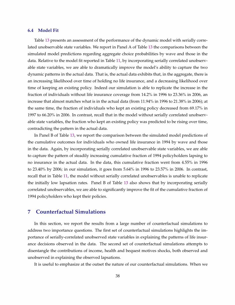
6.4 Model Fit
Table 13 presents an assessment of the performance of the dynamic model with serially corre-
lated unobservable state variables. We report in Panel A of Table 13 the comparisons between the
simulated model predictions regarding aggregate choice probabilities by wave and those in the
data. Relative to the model fit reported in Table 11, by incorporating serially correlated unobserv-
able state variables, we are able to dramatically improve the model’s ability to capture the two
dynamic patterns in the actual data. That is, the actual data exhibits that, in the aggregate, there is
an increasing likelihood over time of holding no life insurance, and a decreasing likelihood over
time of keeping an existing policy. Indeed our simulation is able to replicate the increase in the
fraction of individuals without life insurance coverage from 14.2% in 1996 to 23.36% in 2006, an
increase that almost matches what is in the actual data (from 11.94% in 1996 to 21.38% in 2006); at
the same time, the fraction of individuals who kept an existing policy decreased from 69.17% in
1997 to 66.20% in 2006. In contrast, recall that in the model without serially correlated unobserv-
able state variables, the fraction who kept an existing policy was predicted to be rising over time,
contradicting the pattern in the actual data.
In Panel B of Table 13, we report the comparison between the simulated model predictions of
the cumulative outcomes for individuals who owned life insurance in 1994 by wave and those
in the data. Again, by incorporating serially correlated unobservable state variables, we are able
to capture the pattern of steadily increasing cumulative fraction of 1994 policyholders lapsing to
no insurance in the actual data. In the data, this cumulative fraction went from 4.55% in 1996
to 23.40% by 2006; in our simulation, it goes from 5.64% in 1996 to 23.57% in 2006. In contrast,
recall that in Table 11, the model without serially correlated unobservables is unable to replicate
the initially low lapsation rates. Panel B of Table 13 also shows that by incorporating serially
correlated unobservables, we are able to significantly improve the fit of the cumulative fraction of
1994 policyholders who kept their policies.
7 Counterfactual Simulations
In this section, we report the results from a large number of counterfactual simulations to
address two importance questions. The first set of counterfactual simulations highlights the im-
portance of serially-correlated unobserved state variables in explaining the patterns of life insur-
ance decisions observed in the data. The second set of counterfactual simulations attempts to
disentangle the contributions of income, health and bequest motives shocks, both observed and
unobserved in explaining the observed lapsations.
It is useful to emphasize at the outset the nature of our counterfactual simulations. When we
38

remove the shocks, we are assuming that the market environment faced by consumers remain
unchanged from when all shocks are present. That is, our counterfactual simulation does not
allow for the market to re-equilibrate to respond to the fact that there are now fewer shocks. In
particular, we must assume that the choice set of life insurance contracts that each individual faces
in a given state does not change.
7.1 The Importance of Serially-Correlated Unobserved State Variables
In this section, we report a series of counterfactual simulations to demonstrate the importance
of including serially-correlated unobservable state variables. Panel A of Table 14 is identical to the
bottom sub-panel of Panel B in Table 13 and it reports the model’s predictions about the cumula-
tive outcomes for 1994 policyholders.
In Panel B of Table 14, we report the predictions of the model using the coefficient estimates as
reported in Panel A and B of Table 12, but under the counterfactual assumption that the unobserv-
able state variables did not change over time. It shows that without the shocks to the unobserved
state variables, the model is unable to match the sharply increasing cumulative fraction of 1994
policyholders that lapse to no life insurance, and the model also over-predicts the cumulative
fraction of 1994 policyholders who kept their 1994 coverage.
In Panel C of Table 14, we report the predictions of the model using the coefficient estimates
as reported in Table 12, but under the counterfactual assumption that the observable state variables
stayed the same as their values in 1994, except for age. Surprisingly, assuming away the changes
in the observable state variables barely changes the model’s predictions about the cumulative out-
comes for 1994 policyholders.
In Panel D, we report the predictions of the model using the coefficient estimates of the model
as reported in Panel A and B of Table 12, but under the counterfactual assumption that the neither
the unobservable state variables nor the observed state variables (except for age) change over time.
Only i.i.d choice specific shocks are retained in these simulations. The predictions in Panel D are
very similar to Panel B where only changes in unobservable state variables are eliminated.
The counterfactual simulations in Table 14 thus provide evidence for the importance of serially
correlated unobservable state variables in explaining the choice patterns in the data. Qualitatively,
it plays a much more important role than the variations in the observable state variables in cap-
turing the key features in the data.
39

Table 14: Counterfactual Simulations Using the Estimates of the Dynamic Model withSerially-Correlated Unobservables: Cumulative Outcomes for 1994 Policyholders
Wave
Outcome 1996 1998 2000 2002 2004 2006
Panel A: All shocks included
Lapsed to no life insurance 0.0564 0.0989 0.1286 0.1593 0.1927 0.2357
Changed coverage amount 0.1257 0.1789 0.2111 0.2346 0.2564 0.2783
Kept 1994 coverage 0.8179 0.6922 0.5990 0.5150 0.4385 0.3533
Policyholder died 0.0000 0.0301 0.0614 0.0911 0.1124 0.1328
Panel B: No shocks to the unobserved state variables
Lapsed to no life insurance 0.0462 0.0696 0.0850 0.0981 0.1121 0.1310
Changed coverage amount 0.1260 0.1857 0.2226 0.2512 0.2784 0.3082
Kept 1994 coverage 0.8278 0.7143 0.6294 0.5560 0.4917 0.4195
Policyholder died 0.0000 0.0304 0.0630 0.0947 0.1178 0.1413
Panel C: No shocks to the observable state variables except for age
Lapsed to no life insurance 0.0584 0.1010 0.1307 0.1608 0.1932 0.2354
Changed coverage amount 0.1250 0.1808 0.2132 0.2377 0.2596 0.2826
Kept 1994 coverage 0.8166 0.6881 0.5948 0.5108 0.4355 0.3501
Policyholder died 0.0000 0.0300 0.0612 0.0907 0.1117 0.1319
Panel D: Only i.i.d. choice specific shocks
Lapsed to no life insurance 0.0464 0.0697 0.0847 0.0970 0.1103 0.1280
Changed coverage amount 0.1254 0.1842 0.2206 0.2490 0.2756 0.3047
Kept 1994 coverage 0.8282 0.7157 0.6316 0.5590 0.4959 0.4254
Policyholder died 0.0000 0.0304 0.0631 0.0950 0.1182 0.1419
40
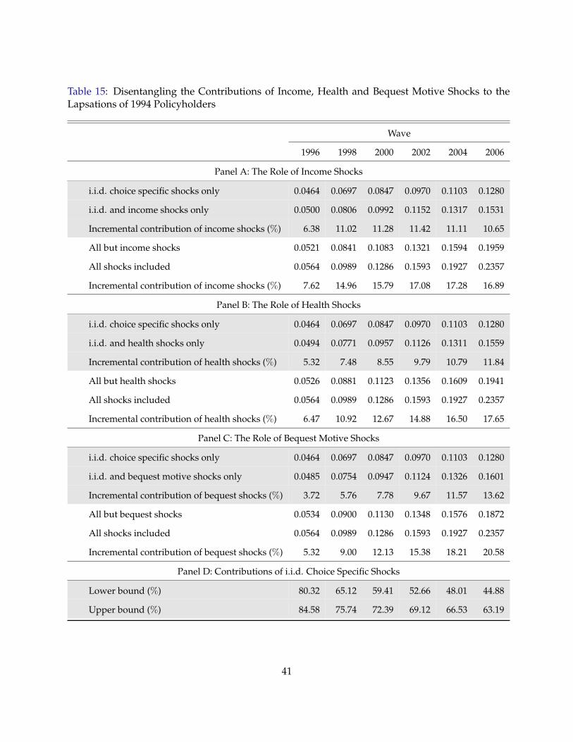
Table 15: Disentangling the Contributions of Income, Health and Bequest Motive Shocks to theLapsations of 1994 Policyholders
Wave
1996 1998 2000 2002 2004 2006
Panel A: The Role of Income Shocks
i.i.d. choice specific shocks only 0.0464 0.0697 0.0847 0.0970 0.1103 0.1280
i.i.d. and income shocks only 0.0500 0.0806 0.0992 0.1152 0.1317 0.1531
Incremental contribution of income shocks (%) 6.38 11.02 11.28 11.42 11.11 10.65
All but income shocks 0.0521 0.0841 0.1083 0.1321 0.1594 0.1959
All shocks included 0.0564 0.0989 0.1286 0.1593 0.1927 0.2357
Incremental contribution of income shocks (%) 7.62 14.96 15.79 17.08 17.28 16.89
Panel B: The Role of Health Shocks
i.i.d. choice specific shocks only 0.0464 0.0697 0.0847 0.0970 0.1103 0.1280
i.i.d. and health shocks only 0.0494 0.0771 0.0957 0.1126 0.1311 0.1559
Incremental contribution of health shocks (%) 5.32 7.48 8.55 9.79 10.79 11.84
All but health shocks 0.0526 0.0881 0.1123 0.1356 0.1609 0.1941
All shocks included 0.0564 0.0989 0.1286 0.1593 0.1927 0.2357
Incremental contribution of health shocks (%) 6.47 10.92 12.67 14.88 16.50 17.65
Panel C: The Role of Bequest Motive Shocks
i.i.d. choice specific shocks only 0.0464 0.0697 0.0847 0.0970 0.1103 0.1280
i.i.d. and bequest motive shocks only 0.0485 0.0754 0.0947 0.1124 0.1326 0.1601
Incremental contribution of bequest shocks (%) 3.72 5.76 7.78 9.67 11.57 13.62
All but bequest shocks 0.0534 0.0900 0.1130 0.1348 0.1576 0.1872
All shocks included 0.0564 0.0989 0.1286 0.1593 0.1927 0.2357
Incremental contribution of bequest shocks (%) 5.32 9.00 12.13 15.38 18.21 20.58
Panel D: Contributions of i.i.d. Choice Specific Shocks
Lower bound (%) 80.32 65.12 59.41 52.66 48.01 44.88
Upper bound (%) 84.58 75.74 72.39 69.12 66.53 63.19
41
7.2 Disentangling the Contribution of Income, Health and Bequest Motive Shocksto Lapsations
In this section, we present a series of counterfactual simulations aimed at disentangling the
contributions of income, health and bequest shocks, including both observed and unobserved
components, to the lapsations of life insurance policies observed in the data. We present our re-
sults in four panels in Table 15. There are two sub-panels in Panels A-C. Let us first discuss Panel
A, which illustrates the contribution of income shocks to the lapsation of 1994 policyholders. In
the shaded sub-panel, we use as baseline the model’s prediction of the cumulative lapsation rates
of 1994 policyholders when only i.i.d choice specific shocks are present (the first row), and exam-
ine how the additional of income shocks to the i.i.d choice specific shocks increases the model’s
predicted lapsation rates (the second row).20 Notice that the addition of income shocks to the i.i.d
choice specific shocks lead to more lapsation. The incremental contribution of income shocks ac-
counts for about 6.38% of the total lapsations predicted by the model when all shocks are included
in 1996.21 The incremental contributions of income shocks over time are reported in the third row.
It reveals that the importance of income shocks are increasing over time in explaining lapsations.
By 2006, income shocks alone were able to explain about 11% of the predicted lapsations.
The bottom, un-shaded, sub-panel in Panel A uses a different baseline. The baseline is instead
the model’s prediction of lapsation rates when all but incomes shocks are included (reported in
the fourth row of Panel A). This baseline prediction is contrasted to the predicted lapsation rates
when all shocks are included (fifth row of Panel A). The difference is attributed to the incremental
contribution of income shocks (sixth row of Panel A). Using this baseline, we see that the contri-
bution of income shocks to lapsation is also increasing over time and eventually income shocks
alone are able to account for about 17% of the predicted lapsations.22
Panel B of Table 15 carries analogous calculations to illustrate the contribution of health shocks
to the lapsations of 1994 life insurance policyholders. The shaded sub-panel shows that if we
use the predicted lapsations with only i.i.d choice specific shocks as the baseline, the incremental
contribution from adding health shocks increases from 5.32% in 1996 to close to 12% in 2006.
20Note that the first row numbers in Panel A of Table 15 are identical to the numbers in the first row of Panel D ofTable 14.
21That is, (0.0500− 0.0464) /0.0564 ≈ 6.38% where 0.0564 is lapsation rates predicted by the model when all shocksare included (reported in the fifth row). The other percentages are calculated analogously.
22There are two other possible counterfactual baselines that we do not report. We could have used “i.i.d choicespecific shock and health shocks” as baseline and contrast it with “i.i.d choice specific shock, health shocks and incomeshocks” (which is the same as “all but bequest motive shocks”). Alternatively, we could have used “i.i.d choice specificshock and bequest motive shocks” as the baseline and contrast it with “i.i.d choice specific shock, bequeest motiveshocks and income shocks” (which is the same as “all but health shocks”). Note that the information needed to carryout these calculations is presented in other rows in Table 15. For space reasons, we do not present these calculationsseparately.
42
If we use the predicted lapsations when all but health shocks are included as the baseline, the
incremental contribution from adding health shocks goes from 6.5% in 1996 to 17.6% in 2006.
Notice that in either baseline, the incremental contributions of health shocks are rising over time.
It seems that income shocks are somewhat more important than health shocks when individuals
are younger (in 1996), but health shocks become as important as, if not more important than,
income shocks by 2006.
Panel C of Table 15 shows the contribution of bequest motive shocks to life insurance lapsa-
tions. As in Panels A and B, the top shaded sub-panel calculates the incremental contribution
of bequest motive shocks using the predicted lapsations with only i.i.d choice specific shocks as
the baseline, and the bottom sub-panel uses the predicted lapsations with all shocks except for
bequest shocks as the baseline. Consistent with the patterns exhibited in Panels A and B, we find
that the importance of bequest motives in explaining lapsation increases over time. It can explain
about 3.7% to 5.3% of the lapsations in 1996, but by 2006, it explains between 13.6% to 20.6% of
the lapsation. Interestingly, our simulations reveal that while income and health shocks may be
slightly more important than bequest motive shocks in explaining the life insurance lapsations for
younger individuals in our sample, bequest motive shocks become a more important determinant
of lapsation when the individuals get older.
Panel D of Table 15 bounds the contributions of i.i.d choice specific shocks in explaining the
lapsations. The lower bounds are calculated as the residuals after subtracting the upper bound
contributions from income, health and bequest motive shocks.23 Panel D reveals that lapsation
of life insurance policies are largely driven by i.i.d choice specific shocks for younger individuals,
but for surviving policyholders an ever larger fraction of lapsations is explained by either income,
or health, or bequest motive shocks. By 2006, between more than 1/3 to more than 1/2 of the
lapsations are driven by one of these shocks.
8 Conclusion
In this paper, we empirically investigate the contributions of income, health and bequest mo-
tive shocks to life insurance lapsations. We present a dynamic discrete choice model of life insur-
ance decisions allowing for serially correlated unobservable state variables. The model is designed
to deal with the data reality where researchers only observe whether an individual has made a new
life insurance decision (i.e., purchased a new policy, or added to/changed an existing policy) but
do not observe the actual policy choice or the choice set from which the new policy is selected.
23For example, we obtain 80.32% lower bound number for year 1996 from 1− 7.62%− 6.47%− 5.32% where 7.62%,6.47% and 5.32% are respectively the upperbound contributions of income, health and bequest motive shocks reportedin Panels A to C. The other bounds are calculated analogously.
43
The semi-structural dynamic discrete choice model allows us to bypass these data limitations. We
empirically implement the model using the limited life insurance holding information from the
Health and Retirement Study (HRS) data.
We deal with serially correlated unobserved state variables using posterior distributions of
the unobservables simulated from Sequential Monte Carlo (SMC) methods. Relative to the few
existing papers in the economics literature that has used similar SMC methods, our paper is, to
the best of our knowledge, the first to incorporate multi-dimensional serially correlated unob-
served state variables. In order to give the three unobservable state variables in our empirical
model their desired interpretations as unobserved income, health and bequest motive shocks, this
paper proposes two channels through which we can anchor these unobservables to their related
observable variables. Useful from a pedagogical perspective, we present our estimation results
separately for a static model without unobservable state variables, as well as for dynamic models
with or without serially correlated unobservable state variables. We illustrate the importance of
serially correlated unobservables by showing the features in the data that a dynamic model with-
out unobservable state variables is unable to capture, and how with unobservable state variables
the model fit dramatically improves (c.f. Tables 11 and 13). We also show that in the model with
unobserved state variables, the contribution of the shocks to unobservables is much larger than
the contribution of the shocks to observed state variables (Table 14).
Our estimates for the model with serially correlated unobservable state variables are sensible
and yield implications about individuals’ life insurance decisions consistent with the both intu-
ition and existing empirical results. In a series of counterfactual simulations reported in Table 15,
we find that a large fraction of life insurance lapsations are driven by i.i.d choice specific shocks,
particularly when policyholders are relatively young. But as the remaining policyholders get
older, the role of such i.i.d. shocks gets less important, and more of their lapsations are driven
either by income, health or bequest motive shocks. Income and health shocks are relatively more
important than bequest motive shocks in explaining lapsation when policyholders are young, but
as they age, the bequest motive shocks play a more important role.
Our empirical findings have important implications regarding the effect of the life settlement
industry on consumer welfare. As shown in theoretical analysis in Daily, Hendel and Lizzeri
(2008) and Fang and Kung (2010a,b), the theoretical predictions about the effect of life settlement
on consumer welfare crucially depend on why life insurance policyholders lapse their policies.
If bequest motive shocks are the reason for their lapsations, then the life settlement industry is
shown to reduce consumer welfare in equilibrium; but if income shocks are the reason for their
lapsations, then life settlements may increase consumer welfare. To the extent that we find both
income shocks and bequest motive shocks play important roles in explaining life insurance lap-
44
sations, particularly among the elderly population targeted by the life settlement industry, our
research suggests that the effect of life settlement on consumer welfare might be ambiguous. Un-
fortunately, our “semi-structural” partial equilibrium model of life insurance decisions and the
life insurance market, which is necessitated by data limitations, is not suited for carrying out a
quantitative evaluation of how the introduction of the life settlement market impacts consumer
welfare, taking into account the presence of both the income-driven and bequest-motive-driven
lapsations. This is an important, but challenging, area for future research.
References
American Council of Life Insurers, “2009 Life Insurers Fact Book,” 2009.
Blevins, Jason, “Sequential Monte Carlo Methods for Estimating Dynamic Microeconomic Mod-
els,” Duke Univeristy Working Paper, 2008.
Chandik, Mark, “The Growing Life Settlement Industry: Is Anyone Watch-
ing Out for Consumers?,” Testimony presented at the California Senate Bank-
ing, Finance and Insurance Committee on Life Settlements, 2008, available at
http://www.sen.ca.gov/ftp/sen/committee/standing/banking/info hearings/backgrounds/2-
20-08 life settlement background.
Daily, Glenn, Igal Hendel, and Alessandro Lizzeri, “Does the Secondary Life Insurance Market
Threaten Dynamic Insurance?,” American Economic Review Papers and Proceedings, 2008, 98 (2),
151–156.
Doucet, Arnaud, Nando de Freitas, and Neil Gordon, Sequential Monte Carlo methods in practice,
New York: Springer, 2001.
Fang, Hanming and Edward Kung, “How does the life settlements market affect the primary
market for life insurance?,” Working paper, 2010a.
and , “The Welfare Effect of Life Settlement Market: The Case of Income Shocks,” Working
Paper, University of Pennsylvania and Duke University, 2010b.
Fernandez-Villaverde, Jesus and Juan F. Rubio-Ramirez, “Estimating Macroeconomic Models: A
Likelihood Approach,” Review of Economic Studies, 2007, 74, 1059–1087.
Fox, Jeremy T, “Semiparametric Estimation of Multinomial Discrete-Choice Models Using a Sub-
set of Choices,” Rand Journal of Economics, 2007, Vol. 38, No. 4, 1002–1019.
45

Gilbert, Jersey and Ellen Schultz, Consumer Reports Life Insurance Handbook, Consumer Reports
Books: Yonkers, NY, 1994.
Gordon, N.J., D.J. Salmond, and A.F.M. Smith, “Novel Approach to Nonlinear/Non-Gaussian
Bayesian State Estimation,” in “IEE Proceedings-F,” Vol. 140 1993, pp. 107–113.
He, Daifeng, “Is Dynamic Selection Present in the Life Insurance Market?,” Working paper, Col-
lege of William and Mary, 2010.
Hendel, Igal and Alessandro Lizzeri, “The Role of Commitment in Dynamic Contracts: Evidence
from Life Insurance,” Quarterly Journal of Economics, 2003, 118 (1), 299–327.
Hong, Han, Ronald A. Gallant, and Ahmed Khwaja, “Estimating a Dynamic Oligopolistic Game
with Serially Correlated Unobserved Production Costs,” Working paper, 2008.
Hu, Yingyao and Matthew Shum, “Nonparametric Identification of Dynamic Models with Unob-
served State Variables,” mimeo, 2009.
Kasahara, Hiroyuki and Katsumi Shimotsu, “Nonparametric Identification of Finite Mixture Mod-
els of Dynamic Discrete Choice,” Econometrica, 2009, Vol. 77, No. 1, 135–175.
Keane, Michael P. and Kenneth I. Wolpin, “The Solution and Estimation of Discrete Choice dy-
namic programming models by simulation and interpolation: Monte Carlo evidence,” The Re-
view of Economics and Statistics, 1994, Vol. 76, 648–672.
Life Insurance Marketing and Research Association, International, “U.S. Indivdiual Life Insurance
Persistency: A Joint Study Sponsored by LIMRA and the Society of Actuaries,” 2009.
McFadden, Daniel, “Modelling the Choice of Residential Location,” in A. Karlqvist, L. Lundqvist,
F. Snickars, and J. Weibull, eds., Spatial Interaction Theory and Planning Models, 7 North Holland:
Amsterdam, 1978, Vol. I, 75–96.
Norets, Audriy, “Inference in Dynamic Discrete Choice Models with Serially Correlated Unob-
served State Variables,” Econometrica, 2009, Vol. 77, No. 5, 1665–1682.
Olsson, J. and T. Ryden, “Asymptotic Properties of Particle Filter-Based Maximum Likelihood
Estimators for State Space Models,” Stochastic Processes and their Applications, 2008, 118 (4), 649–
680.
46