why is high capacity utilization no longer inflationary in canada

8/14/2019 Why is High Capacity Utilization No Longer Inflationary in Canada

http://slidepdf.com/reader/full/why-is-high-capacity-utilization-no-longer-inflationary-in-canada 1/47

December 16, 2005

Department of Finance

Ministère des Finances

Working Paper

Document de travail

Why Is High Capacity Utilization No Longer Inflationary in Canada

by

Chetan Dave * Department of Economics, University of Texas at Dallas

Faculty of Social Sciences, Richardson, TX. 75083 U.S.A.

[email protected]

Workin Pa er 2006‐02

* I would like to thank Max Baylor, Mireille Laroche, Chris Matier, Bing-Sun Wong and Benoît Robidoux as

well as seminar participants at Finance Canada and the University of Pittsburgh. All remaining errors are mineand comments are welcome. This paper was written in part while the author was in residence at the Economic

Studies and Policy Analysis Division of the Department of Finance Canada, the author is currently an Assistant

Professor at the University of Texas at Dallas. Usual caveats apply.

Working Papers are circulated in the language of preparation only, to make analytical work undertaken by the staff of the

Department of Finance available to a wider readership. The paper reflects the views of the authors and no responsibility for

them should be attributed to the Department of Finance. Comments on the working papers are invited and may be sent to the

author(s). Les Documents de travail sont distribués uniquement dans la langue dans laquelle ils ont été rédigés, afin de rendre le

travail d’analyse entrepris par le personnel du Ministère des Finances accessible à un lectorat plus vaste. Les opinions qui

sont exprimées sont celles des auteurs et n’engagent pas le Ministère des Finances. Nous vous invitons à commenter les

documents de travail et à aire arvenir vos commentaires aux auteurs.



2



1 Introduction

Industrial capacity utilization measures are viewed by monetary authorities as useful

inflationary indicators. As a resource utilization measure, capacity utilization is defined as

the ratio of actual to capacity output, where the latter quantity is typically estimated with

one of several available filtering techniques. In Canada, the aggregate capacity utilization

series is benchmarked to survey data, providing a unique opportunity to examine aggregate

data that reflect actual business conditions1. However, recently for Canada, capacity uti-

lization levels have been high without inducing increases in core CPI inflation. Figure 1 in

Appendix B provides a plot of capacity utilization and core CPI inflation. The plot suggests

that through time the relationship between capacity utilization and core CPI inflation may

have diminished in terms of levels and/or co-movements. Further, in recent years, the series

has breached the well accepted level of the non-accelerating inflationary rate of capacity

utilization (NAICU) of 82% without corresponding increases in core CPI inflation2.

These observations prompt two natural questions: is high capacity utilization no longer

inflationary, and if not, why? This paper addresses these questions by first establishing

relevant stylized facts drawn from empirical models of capacity utilization-inflation Phillips

curves. The estimation results indicate that the eff ect of capacity utilization on inflation has

diminished over time, and that there are statistically significant breaks in the relationship.

1See Fixed Capital Flows and Stocks (Statistics Canada) for details on the construction of aggregatecapacity utilization series using survey responses. The relevant survey is the Capital Expenditures Surveythat requests firms to answer the following question. “For the year [t], this plant operated at what percentageof its capacity?”, [where], “Capacity is defined as maximum production attainable under normal conditions.With regard to normal conditions, please follow the company’s operating practices with respect to the use of productive facilities, overtime, workshifts, holidays, etc. When any of your facilities permit the substitutionof one product for another, use a product mix at capacity which is most similar to the composition of your[year t] output.”

2See Baylor (2001) for a detailed discussion.

1



These breaks correspond to economic events that can be interpreted as having increased

the degree of competitiveness and, to a lesser extent, decreased the level of nominal rigidi-

ties in the Canadian economy. In order to qualitatively lend credence to this conjecture,

this paper estimates the dynamic stochastic general equilibrium model of Ireland (2003).

The model incorporates monopolistically competitive firms who face time-varying cost-push

shocks and Rotemberg (1982) style nominal menu costs of adjusting prices. As a result,

the model delivers a capacity utilization-inflation trade-off that is in part a function of the

degree of competitiveness and nominal rigidities present in the economy. The empirical ex-

ercise demonstrates that the estimated aggregate price mark-up may have decreased, as may

have the degree of nominal rigidity in the Canadian economy, lending credence to the conjec-

tures behind the observed breaks in the capacity utilization-inflation relationship. The main

conclusion is that the Canadian economy may be better represented by characterizations

provided by competitive equilibrium flexible price models which do not necessarily predict a

structural relation between inflation and real resource utilization measures.

The remainder of the paper is structured as follows. In Section 2, empirical models of the

capacity utilization-inflation Phillips curve are specified under the assumption that inflation

expectations are backward looking. Additionally, the assumption that these expectations

may also be forward looking is also made, given that the Bank of Canada and the Gov-

ernment of Canada jointly adopted an inflation targeting regime in the early 1990’s. The

specifications take the form of time-varying parameter models (as per Kim & Nelson (1999)),

single structural break models (as per Hansen (2000)) and multiple structural break models

(as per Bai & Perron (1998)). Estimation results, presented in Section 3, suggest that there

is a steady deterioration in the capacity utilization-inflation relationship through time.

2



The central conjecture in this paper on the reasons driving the stylized facts, is that

the Canadian economy has become more competitive and, to a lesser extent, faces reduced

nominal rigidities. An explanation of a leading positive relationship between capacity uti-

lization and inflation is as follows. If firms are monopolistic competitors then when faced

with, say, a positive demand shock, they will ratchet up production given fixed capacity.

Increased production will drive up costs, which will be passed on to consumers through the

price-setting power of firms resulting in an increase in inflation. This increase in inflation

would be associated with high capacity utilization as a result of the increase in production

relative to capacity. However, if firms are competitive then they will be less able to pass on

cost increases, reducing the eff ect on inflation3. In Section 4 of this paper a micro-founded

New Keynesian model by Ireland (2003) is described that captures this intuition. In Section

5, the model is estimated and demonstrates that the aggregate price mark-up has decreased,

and that the degree to which nominal rigidities are present may have decreased. As a result,

the statistical findings of Section 3 are validated by model estimates and the paper concludes

in Section 6 with a summary of the stylized facts drawn and the explanations given for them.

The remainder of this section outlines some related research.

The analysis in this paper also acts as an application of an emerging synthesis between

New Keynesian and ‘real’ business cycle models. Indeed Clarida, Gali & Gertler (2000) and

Ireland (2002, 2003) among others attempt to marry the advantages aff orded by real business

cycle transmissions of technology and preference shocks with non-Walrasian shocks, such as

3See Shapiro (1989) for details on the two transmission mechanisms and a early introduction to theissue of capacity utilization-inflation dynamics for the United States. Finn (1996) demonstrates that acompetitive equilibrium model with a role for energy shocks adequately explains the capacity utilization-inflation relationship for the United States.

3



the cost-push shocks considered in the present analysis4. This synthesis is emerging as

fertile ground, with strong micro-foundations5, to sort out the competing sources of business

cycle fluctuations, and this paper adds to the synthesis by analyzing a relationship between

inflation and a macroeconomic variable that results from a comprehensive survey of firms.

1.1 Related Literature: Capacity Utilization & Inflation

An early discussion of the relationship between capacity utilization and inflation is

provided by Shapiro (1989) for the United States. Two of the major questions discussed

are whether, on an industry-by-industry basis, output growth is constrained when capacity

utilization is high and whether price increases follow. The answers are provided having

discussed the many shortcomings of capacity utilization measures for the United States6. In

brief, Shapiro (1989) finds that high utilization levels do not imply constraints on output

growth. Further, relative prices and markups do not seem to increase when utilization is

high. Overall, the empirical results suggest that,

“High measured utilization does not imply that the economy has hit a barrier

to further growth or that capital is scarce. Consequently, high measured utiliza-

4The literature often considers two competing paradigms for analyzing the types of shocks that generatebusiness cycles in explicit dynamic, stochastic, general-equilibrium models. The real business cycle literaturefocuses on the role of ‘fundamental shocks’ such as technology and demand shocks, along with the assumptionthat markets clear and that there is never any underemployment of resources. In contrast, the New Keynesianliterature acknowledges the importance of fundamental shocks but does not require perfect competition and

market clearing. Instead, the New Keynesian literature suggests that in addition to fundamental shocks,there are non-Walrasian shocks to an imperfect market structure that aid in propagating business cycles.One such shock is that to the elasticity of demand of intermediate input firms who are assumed to bemonopolistic competitors. These shocks are termed non-Walrasian or cost-push shocks.

5Here micro-foundations refer to the fact that New Keynesian models now specify IS and Phillips curvesbased on explicit optimization given assumptions, versus ad-hoc specifications of these relations.

6The measures employed in the United States diff er significantly from those in Canada. In the U.S.information from several, possibly non-comprehensive, surveys is used as well as a mix of interpolationand forecasting techniques (see Shapiro (1989)). The methodology employed by Statistics Canada is moreuniform, as witnessed by the methodology section of Fixed Capital Flows and Stocks (Statistics Canada).

4



1.2 Related Literature: The Output Gap & Inflation

The Bank of Canada’s measure of the output gap and Statistics Canada’s measure of

capacity utilization are clearly related utilization measures. The qualitative information

contained in the two time series goes beyond a theoretical similarity. Figure 2 in Appendix

B plots both series and the figure indicates that the two series track one another surprisingly

well despite a major diff erence in the two series. Specifically, whereas it is not abundantly

clear how the output gap is estimated, aggregate capacity utilization benchmarked to survey

data, and can be argued to reflect real world business conditions7.

Analysis of the output gap-inflation relationship has been thoroughly conducted in a

series of papers by the Bank of Canada. The most recent research is conducted by Demers

(2003) who finds breaks in the output gap-inflation Phillips curve. Indeed using the multiple

break tests of Bai & Perron (1998) and a three-regime Markov switching model, Demers

(2003) rejects linearity and parameter constancy in the output gap-inflation relationship.

However, little structural interpretation is off ered beyond the role of monetary policy. While

it is plausible that the inflation targeting regime instituted by the Bank of Canada has led

to low and stable inflation, with expectations anchored at the target of 2%, the Canadian

economy has also experienced other important institutional changes over the years. Indeed,

Baylor (2001) suggests that with respect to the capacity utilization-inflation relationship, “an

increasingly global economy, rapid technological progress, and a more preemptive monetary

policy” may provide possible explanations of the break. These explanations are explored in

7Data for the output gap were obtained from Demers (2003), those for capacity utilization were obtainedfrom CANSIM as detailed in the following section. Here the qualifier aggregate for capacity utilizationrefers to total industrial as opposed to economy-wide and it is of note that only the manufacturing sector issurveyed for capacity utilization.

6



the present analysis by incorporating the role of cost-push shocks simultaneously with the

role of technology shocks in driving the capacity utilization-inflation Phillips curve; while

allowing for a flexible Taylor rule specification to approximate monetary policy. Therefore

the present analysis encompasses, to an extent, the empirical research on the output gap-

inflation relationship and the results can be viewed as a complement to those discussed in

Demers (2003).

2 Empirical Models

In order to determine whether there has been a break over time in the statistical re-

lationship between capacity utilization and inflation, continuous and discrete break tests

must also be robust across assumptions on inflation expectations. Within the time period

considered in this section, 1975QI-2002QIV, the Bank of Canada implemented three main

changes in monetary policy. First, in 1975, the Bank introduced the policy of gradualism,

that is, controlling inflation through gradual reductions in M1 growth. Second, in the 1980’s,

the Bank of Canada instituted policy changes in order to reduce the high and variable infla-

tion Canada had experienced in previous decades (Longworth (2002)). Third, the Bank of

Canada instituted an inflation targeting regime in 1991QI and since then has moved towards

a regime of ‘credible’ inflation targeting (Longworth (2002)). Therefore two types of mod-

els are specified: a backward looking model and a mixture model that combines backward

looking and forward looking inflation expectations.

7



2.1 Backward Looking Expectations

Consider the standard predictive capacity utilization-inflation Phillips Curve8,

πt = α0 + α1ut−1 + πet (2.1)

where πt represents inflation, ut represents capacity utilization and πet represents expected

inflation. The backward looking expectations assumption specifies inflation expectations as

a lag over past inflation, with the lag coefficients summing to unity. A lag specification often

employed for Canada (see Johnson (2002), Longworth (2002) and references therein) yields,

πt = α0 + α1ut−1 + α2πt−1 + α3πt−2, α2 + α3 = 1 (2.2)

The unconstrained equation (2.2) yields the following backward looking expectations empir-

ical specification,

πt = α0 + α1ut−1 + α2πt−1 + α3πt−2 + α4xt−1 + ε1t (2.3)

where xt−1 is the lagged change in the Canada-U.S. real exchange rate that is included to

account for the small and open nature of the Canadian economy.

8

See Emery & Chang (1997) and references therein for a background on utilization-inflation Phillipscurves that have been estimated in the literature.

8



2.2 Mixture Expectations

Under the assumption of mixture expectations there is weight on forward looking ex-

pectations, thus the analog of (2.2) is given by,

πt = α0 + α1ut−1 + α2πt−1 + α3πt−2 + α5πet , α5 = 1− α2 − α3 (2.4)

where πet represents period t’s expectation of inflation for period t +1 and is a measured vari-

able9. The unconstrained version of (2.4) yields the following mixture expectations empirical

specification,

πt = α0 + α1ut−1 + α2πt−1 + α3πt−2 + α4xt−1 + α5πet + ε2t (2.5)

which can be interpreted as nesting the backward looking model. Indeed, the models are

specified without restricting them to their respective inflation expectations assumptions as

it is assumed that no one set of assumptions on expectations can reflect reality. Further, by

estimating unrestricted versions it can be seen to what extent forward looking expectations

matter by verifying whether the estimate of α5 is significant and positive.

In order to determine whether the relationship has deteriorated under backward looking

9Data were obtained from the Conference Board of Canada’s survey of forecasters to proxy for TotalInflation expectations. As this time series begins in 1975QI, the analysis was conducted for the sample

period 1975QI-2002QIV. Alternate series for inflation expectations, constructed from actual inflation rates,does allow for a longer time dimension, however, yields the same qualitative results. The main advantageof the survey series is that it allows the model to incorporate actual expectations. The remaining data oncore CPI inflation (i.e. inflation less the influence of indirect taxes, energy and other volatile components),capacity utilization and exchange rates were obtained or constructed from: CANSIM series v4331081, v37426& v1997756, Baylor (2001), Demers (2003) and RFABASE series PDIGDPUS. Finally, the data on capacityutilization were augmented by data obtained from Statistics Canada (Investment and Capital Stock Division,unpublished) since CANSIM series v4331081 is available only starting in 1987.

9



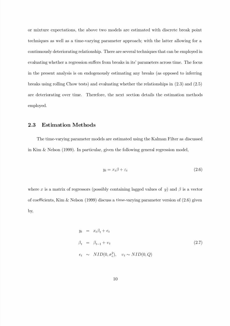
or mixture expectations, the above two models are estimated with discrete break point

techniques as well as a time-varying parameter approach; with the latter allowing for a

continuously deteriorating relationship. There are several techniques that can be employed in

evaluating whether a regression suff ers from breaks in its’ parameters across time. The focus

in the present analysis is on endogenously estimating any breaks (as opposed to inferring

breaks using rolling Chow tests) and evaluating whether the relationships in (2.3) and (2.5)

are deteriorating over time. Therefore, the next section details the estimation methods

employed.

2.3 Estimation Methods

The time-varying parameter models are estimated using the Kalman Filter as discussed

in Kim & Nelson (1999). In particular, given the following general regression model,

yt = xtβ + εt (2.6)

where x is a matrix of regressors (possibly containing lagged values of y) and β is a vector

of coefficients, Kim & Nelson (1999) discuss a time-varying parameter version of (2.6) given

by,

yt = xtβ t + et

β t = β t−1 + υt (2.7)

et ∼ NID(0, σ2e), υt ∼ NID(0, Q)

10



The inferential focus is on the estimates of the standard deviation of each of the time-varying

parameters (where Q is the diagonal variance-covariance matrix); the resulting time varying

estimates (

bβ t); and model’s conditional variances and forecast errors which identify periods

of volatility. The backward looking and mixture models presented above are estimated using

this general framework.

While time-varying parameter estimation evaluates the presence of any continuous breaks,

inference can be strengthened with discrete breaks tests. If there are any shifts then struc-

tural break models can be used to date them. For this purpose, the methods of Hansen

(2000) and Bai & Perron (1998) are employed to identify structural breaks. The inferential

focus in Hansen (2000) is on identifying one possible break over time in a model such as that

in (2.6), whereas the inferential focus in Bai & Perron (1998) is on the following four types

of break tests. The first is a test of zero versus a specific number of breaks (say, k), denoted

the sup F (0|k) tests. The second type, denoted the D max tests are tests of no breaks versus

an unknown number of breaks. The third type of tests are for the null of k breaks versus

k + 1 breaks in the model. The fourth type, which are most useful in the present context,

are those that estimate any breaks sequentially. The next section presents the estimation

results using these methodologies for identifying discrete and continuous breaks.

3 Estimation Results

Table 1 in Appendix A presents the results of estimating equations (2.3) and (2.5) using

Hansen’s (2000) methods assuming a single break. For the backward looking model, the

estimated break date (1982QIV) has a relatively narrow 95% confidence interval (1982QII-

11



1983QI) and a good fit (as the joint R2 of the model with one break at 1982QIV is 0.819).

However, in these results, the pre-break estimate of the coefficient on capacity utilization

(α1) is rather weak and the post-break estimate is more significant; however, this could be

a feature of the short pre-break sample. The estimates for the mixture model are stronger

in that the estimate for the coefficient on inflation expectations (α5) is significant in the

overall and pre-break sample. In the post-break sample, the significance of α5’s estimate

falls, reflecting in part the low variability of inflation expectations over that time period as

exhibited in Figure 3 of Appendix B. The main single break estimation result for the mixture

model is the break date of 1983QIV with a large confidence interval of 1982QII-1991QII which

is suggestive of multiple breaks. Finally, Table 1 confirms a decreasing estimate of α1 from

0.223 (pre-break) to 0.095 (post-break) with the former being the more significant estimate

in the mixture model. Overall, the results presented in Table 1 suggest breaks in both the

backward looking and mixture models with possibly a decreasing coefficient on capacity

utilization across the breaks.

Multiple break tests following Bai & Perron (1998) are presented in Table 2 of Appen-

dix A. The sup F (0|k) tests reject the null of no breaks for the alternative of k possible

breaks across the board (k = 1 to 5) for both the backward looking and mixture models.

The same holds for the D max tests of no breaks versus the null of an unknown number

of breaks. The sup F (k + 1|k) tests of the null of k breaks versus the alternate of k + 1

breaks suggest two breaks for the backward looking model and three for the mixture model.

The estimation of sequential breaks finds two breaks for the backward looking model that

corresponds to the 1981-1982 recession (1982QII-1983QIII), and the adoption of the inflation-

targeting regime in 1991 (1990QI-1991QIII). For the mixture model, three breaks are esti-

12



as specified in (2.7), the initial values in the Kalman Filter can be set to an arbitrary value

with large initial uncertainty, hence the results assuming a diff use prior are reported in Table

3 and in Figures 4-6.

Overall, the results suggest discrete breaks along with a continuous deterioration in the

utilization-inflation relationship. In addition, the data prefer a model that incorporates

forward looking behavior. Finally, the results may be interpreted within the context of

recent Canadian economic history. In a nutshell, this history can be summarized by three

main inter-related and overlapping changes in the governments’ policies, namely changes in

monetary and fiscal regimes and freer trade within North America. After the excesses of the

1970’s, the Bank of Canada was said to be committed to a transparent monetary policy that

ensured low and stable inflation. This commitment resulted in the initial deflation of the

1980’s and the subsequent move to inflation targeting in the late 1980’s and the early 1990’s.

Indeed, Longworth (2002) outlines the resulting benefits stemming from reduced inflation

uncertainty:

“The reduced uncertainty about inflation seems to have had a number of

significant benefits. First, it seems to have led to a decline in relative wage

variability because of less disagreement about the inflation outlook, therefore

leading to a better allocation of labour. Second, it certainly has made planning

easier and has led to longer labour and financial contracts, which means lower

transactions and bargaining costs for firms and households. Third, it has likely

been an important factor in a reduction of days lost to labour disruptions. Fourth,

it means that there is less need to protect oneself against unexpected inflation,

14



which is a real saving of resources. Fifth, it has been a factor leading to the

development of more complete financial markets (with longer-term instruments),

which allows a greater diversification of risks at lower cost. Finally, it has been

associated with less variable interest rates, which, in turn, have led to lower

capital losses and gains on bonds, and have tended to lead to lower risk premiums

on longer-term instruments.”

These benefits could be interpreted as having decreased the degree of nominal rigidity. In

addition, fiscal stability can lead to a better allocation of resources due to reduced uncertainty

about aggregate fiscal policies. Such stability was obtained by a move to eliminate high

deficits, surpluses were indeed finally reported in fiscal year 1997-1998 and remain thereafter.

Finally, the process of free trade should decrease the significance of cost-push shocks as

firms compete to satisfy aggregate demand. For Canada, free trade not only opened the vast

markets of the United States but also led to increased competitive pressures from firms in the

United States. Indeed, the free trade process began with the Free Trade Agreement in the

late 1980’s and continued through the 1990’s with the signing of NAFTA. Other structural

reforms have also occurred in Canada in the late 1980’s and through the 1990’s that may have

triggered more competition in labour and product markets such as the restructuring of the

Employment Insurance and social assistance programs and reduced burdensome regulations

in domestic markets as well as vis-à-vis foreign investment13. It would therefore seem that a

reasonable conjecture is that these increased competitive pressures and decreased rigidities

should have led to an uncoupling between real resource utilization and inflation in Canada

13See Alsenia et al. (2003), Golub (2003) and Nicoletti & Scarpetta (2003).

15



through the 1980s and 1990s.

In order to verify this conjecture, a model is required that predicts a relationship between

capacity utilization and inflation due in part to nominal rigidities and cost-push pressures.

That is, the model must capture the intuition outlined in the Introduction (as adapted

from Shapiro (1989)). Given such an environment, empirical evaluation of the model must

show that an uncoupling between real resource utilization and inflation may occur if the

significance of cost-push shocks decreases relative to ‘fundamental’ shocks such as technology

and demand shocks. Such an environment is provided within the New Keynesian literature

that allows for cost-push shocks to compete with ‘fundamental’ shocks in the data; in addition

the literature is able to account for both backward looking and forward looking behavior.

The next section describes one such model and evaluates it empirically to lend credence to

the above conjecture.

4 Monopolistic Competition and Capacity Utilization

The previous section argued that the adoption of a sound monetary and fiscal policy

framework, together with freer trade and other significant structural reforms may have had

an eff ect on the capacity utilization-inflation relationship. In particular, these institutional

changes can be interpreted as mapping into increased competition and decreased rigidities in

the economy. This section outlines a model of imperfect competition with sticky prices, and

then estimates the model in order to possibly lend credence to this conjecture. The model

is provided by Ireland (2003) and is indeed a standard in the literature.

16



4.1 The Basic Environment

The aggregate economy, operating in discrete time, is assumed to consist of a repre-

sentative household, a finished goods firm, a continuum of intermediate inputs firms and a

central bank. The intermediate inputs firms each produce a diff erentiated output used in

the production of the final good. The details of the basic environment are as follows.

4.1.1 Households

Households are assumed to maximize utility defined over consumption (C t), money

(M t) and the disutility of labor (N t). The representative household’s optimization objective

is given by,

M ax. U = E 0

∞X0

β t½

at log C t + log M t

P t−

N ηt

η

¾ (4.1)

s.t. P tC t + Bt

Rt

+ M t = M t−1 + Bt−1 + T t + W tN t + Dt (4.2)

β ∈ (0, 1), η ≥ 1 (4.3)

where β has the usual rate of time-preference interpretation and at is a demand shock. In

the specification of the budget constraint (4.2) above, it is assumed that the household holds

bonds (B) and money, where the former matures at a gross nominal rate of Rt between two

discrete time periods. The household also receives transfers (T ) from the monetary authority

and works in order to earn wages (W ) to meet its’ expenditures. Finally, the household is

assumed to own the intermediate inputs firms and thus receives a dividend payment from

the firms in each period (D). The solution to the households problem yields a demand for

17



money balances, supply of labor and a demand for the final consumption good, as follows,

M t

P t=

C tRt

at(Rt − 1) (4.4)

C tN η−1t =

atW t

P t(4.5)

βE t

½ at+1

P t+1C t+1

¾ =

at

P tC tRt

(4.6)

These first order conditions along with the budget constraint are the first in a system of

equations that will characterize the aggregate economy.

4.1.2 Firms

There are two types of firms, one that produces a final consumption good and a con-

tinuum of intermediate inputs firms that supply inputs to the final consumption good firm.

The final good firm is assumed to operate in a competitive environment and thus solves the

following static problem,

Max. ΠF t = P tY t −

1Z 0

P itY itdi (4.7)

s.t. Y t =

⎧⎨⎩

1Z 0

Y θt−1

θt

it di

⎫⎬⎭

θtθt−1

(4.8)

18



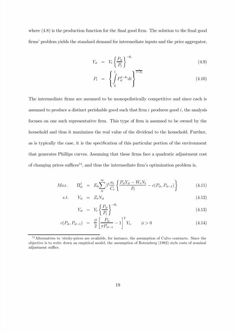
where (4.8) is the production function for the final good firm. The solution to the final good

firms’ problem yields the standard demand for intermediate inputs and the price aggregator,

Y it = Y t½P it

P t¾−θt (4.9)

P t =

⎧⎨⎩

1Z 0

P 1−θtit di

⎫⎬⎭

1

1−θt

(4.10)

The intermediate firms are assumed to be monopolistically competitive and since each is

assumed to produce a distinct perishable good such that firm i produces good i, the analysis

focuses on one such representative firm. This type of firm is assumed to be owned by the

household and thus it maximizes the real value of the dividend to the household. Further,

as is typically the case, it is the specification of this particular portion of the environment

that generates Phillips curves. Assuming that these firms face a quadratic adjustment cost

of changing prices suffices14, and thus the intermediate firm’s optimization problem is,

Max. ΠI it = E 0

∞X0

β t at

C t

½P itY it −W tN t

P t− c(P it, P it−1)

¾ (4.11)

s.t. Y it = Z tN it (4.12)

Y it = Y t

½P it

P t

¾−θt

(4.13)

c(P it, P it−1) = φ

2

∙ P it

πP it−1− 1

¸2Y t, φ > 0 (4.14)

14Alternatives to ‘sticky-prices are available, for instance, the assumption of Calvo contracts. Since theobjective is to write down an empirical model, the assumption of Rotemberg (1982) style costs of nominaladjustment suffice.

19



where Z t is a technology shock and φ measures the speed of adjustment of prices and hence

the degree of nominal rigidity. The solution to the intermediate firms’ problem yields,

0 = θt

1− θt

µP it

P t¶ 1

θt−

1 Y tat

P tC t+ at

1− θt

µP it

P t¶ θt

θt−

1 W t

P t

Y t

Z t1

P tC t(4.15)

−φ

∙ P it

πP it−1− 1

¸ Y tat

πP it−1C t+ βφE t

µat+1

at

µ P it

πP it−1− 1

¶ Y tP it+1

πP itP it

¶

as the first order condition in which price dynamics are induced by the assumed degree of

nominal rigidity.

4.1.3 Stochastic Assumptions and Equilibrium Conditions

There are three types of shocks in this economy, namely, demand shocks, technology

shocks and cost-push shocks. Demand shocks (at), technology shocks (Z t) and cost-push

shocks (θt) are assumed to all have steady state values a, z and θ that are larger than unity.

All shocks are assumed to evolve as per the following logarithmic processes.

log(at) = (1− ρa)log(a) + ρa log(at−1) + εat, a > 1

log(Z t) = log(z ) + log(Z t−1) + εzt, z > 1

log(θt) = (1− ρθ)log(θ) + ρθ log(θt−1) + εθt, θ > 1

Equilibrium in this model is characterized by symmetry,

Y it = Y t, N it = N t, P it = P t, Dit = Dt (4.16)

20



Money and bond markets clear so that,

M t = M t−1 + T t (4.17)

Bt = Bt−1 = 0 (4.18)

The only remaining required features of the model are a Taylor rule, to represent the

activities of the central bank, and a specification for capacity utilization.

4.2 Capacity Utilization

Capacity utilization is typically defined to be the ratio of actual to capacity output (Y t,

see Shapiro (1989)). Here capacity output is defined to be the efficient level of output, which

is equivalent to claiming that it would be the level of output chosen by a benevolent social

planner who would solve,

M ax. U = E 0

∞X0

β t

⎧⎨⎩at log Y t −

1

η

⎛⎝ 1Z

0

N itdi

⎞⎠η⎫⎬⎭ (4.19)

s.t. Y t = Z t

⎛⎝

1Z 0

N θt−1

θt

it di

⎞⎠

θtθt−1

(4.20)

The solution to the problem yields an expression for capacity output implying that another

equation can be added to the system so far, namely the specification of capacity utilization,

U t = Y t

a1

η

t Z t

(4.21)

21



The definition of capacity utilization here is very similar to the definition of an output gap,

indeed the two are the same in this environment. In order to ensure that this is a reasonable

specification, Figure 2 in Appendix B plots the two series and as can be seen in the figure,

there is very little diff erence between the ratio (U t) and the diff erence (the output gap)15

measures.

4.3 The Equilibrium System

The equilibrium system consists of the first order conditions of the household, its’ budget

constraint, the aggregate production function having imposed symmetry, the aggregate real

dividends from the intermediate input firms to the households and the first order condition

of the intermediate inputs firms. The system can be normalized by Z t and wages, money,

labor, dividends and capacity output can be eliminated. The steady states of those variables

not specified exogenously are given by,

R = zπ

β , C = Y =

µa

θ − 1

θ

¶ 1

η

, U =

µθ − 1

θ

¶ 1

η

(4.22)

15The output gap series was obtained from the Bank of Canada for the time period 1975QI-2002QIV fromDemers (2003).

22



Employing these steady states in log-linearizing the system yields the following form,

at = ρaat−1 + εat, εat ∼ NID(0, σ2a), |ρa| < 1 (4.23)

ut = yt − ωat, ω = η−1 (4.24)

ut = αxut−1 + (1 − αx)E tut+1 − (rt −E tπt+1) + (1− ω) (1− ρa)at (4.25)

θt = ρθθt−1 + εθt, εθt ∼ N ID(0, σ2θ), |ρθ| < 1 (4.26)

πt = βαππt−1 + β (1− απ)E tπt+1 + η(θ − 1)

φ ut −

1

φθt (4.27)

gt = yt − yt−1 + z t → g = z (4.28)

z t = εzt, εzt ∼ NID(0, σ2z) (4.29)

rt = ρrrt−1 + ρππt + ρggt + ρuut + εrt, εrt ∼ NID(0, σ2r) (4.30)

where all variables are in log deviations fromtheir steady states, that is, xt = log(X t)−log(X )

where X is the steady state value of the variable X t. Next, the additional parameters of αx ∈

[0, 1] and απ ∈ [0, 1] have been introduced in addition to the deep parameters of the model.

These two additional parameters have been introduced in order to augment the system

with lagged terms, as typically these lagged terms have an influence in real data, setting

αx = απ = 0 yields the original micro-foundations. Equations (4.23), (4.26) and (4.29)

describe the shock processes for demand, cost-push and technology shocks, respectively.

Equation (4.25) is the familiar IS curve, and equation (4.27) is the Phillips curve. Finally,

equation (4.30) is the Taylor rule followed by the central bank. Here, it is assumed that the

monetary authority reacts to inflation, the observable growth rate of output (gt) and capacity

utilization. In addition, the above model can be simplified by letting the cost-push shock be

23



defined as et = 1φ

θt implying that ρe = ρθ and σe = 1φ

σθ. Indeed, it is important to note that

this transformation does not alter the interpretation of the cost-push shock process under the

assumption that all disturbances are Gaussian in nature. The transformation simply assists

in estimating the systems parameters. The following is a summary of the main parameters

of interest and their interpretation.

Parameter Interpretation

φ Degree of price rigidity.

θ 1θ−1

is the steady state mark-up.

ρθ Degree of persistence of cost-push shocks (ρe when φ fixed).

σθ Variance of cost-push shock process (σe when φ fixed).

η Degree of disutility of labor, ω = η−1

ψ ψ = η(θ−1)φ

is the overall response of inflation to utilization.

The main conjecture in this paper is that the aggregate Canadian economy has become

increasingly competitive after 1984QII, and that the economy may also be facing reduced

nominal rigidities after that break as well16. Within the context of the model above, demon-

strating the validity of this conjecture translates into demonstrating that the steady state

price mark-up¡ 1θ−1

¢ and the degree of price rigidity (φ) have decreased conditional upon

any changes in the curvature of the disutility of labor function as measured by η; given that

the influence of utilization on inflation is given by ψ = η(θ−1)

φ in the Phillips curve. Thus,

maximum likelihood methods are employed in the next section to estimate the parameters.

16This date corresponds to the endpoint of the 95% confidence interval of the first break in the mixturemodel noted in Table 2. Alternatively, one could also consider estimating the model across the 1991 break;however, due to a small sample post-break this was not done as the small sample causes the Kalman Filterused to estimate the deep parameters to not have enough observations. In future work, Bayesian techniquescould be used to address this and other issues.

24



Finally, it is instructive to note that the definition of capacity utilization above is diff erent

from that typically assumed in the literature. The analysis of capacity utilization as a

propagation tool has received attention from several researchers. Wen (1998) builds a real

business cycle model with a depreciation-in-use definition of capacity utilization in order

to demonstrate that the resulting propagation mechanism is sufficient to explain several

aspects of the U.S. business cycle. Unlike Wen (1998), in this paper capacity utilization is

defined as the ratio of choices under decentralized and social planner problems, with the

result that capacity utilization moves in response to technology and demand shocks. The

depreciation-in-use assumption is also evaluated by Fagnart et al. (1999) in a model with

imperfect markets. They focus on the diff erence between capacity utilization and capital

utilization. In their economy, monopolistic firms use putty-clay technologies and react to

demand shocks. As a result, they are able to demonstrate that some firms may idle and

why utilization rates may diff er across firms. The analysis in this paper can therefore be

interpreted as being complementary to those of Wen (1998) and Fagnart et al. (1999). The

main diff erence being that here an explicit characterization with respect to market structure

is being sought as the conjecture is that increased competition, all things equal, will lead this

variable to potentially lose its’ link with inflation. Indeed Corrado & Mattey (1997) discuss

the link between capacity utilization and inflation for the United States in detail. They

outline the explanations behind the link between high capacity utilization and inflation, and

also provide a discussion of the practicalities of the measurement of this statistic for the

United States. However, in Canada, the transmission of high capacity utilization to inflation

may be breaking down using aggregate benchmarked to surveys which provides a unique

inflationary indicator.

25



5 Model Evaluation

The model in the previous section could conceivably be simulated given calibrated values

for parameters. However, assuming values for the parameters of the Taylor rule can be a

questionable proposition. This is in part due to the instability of the Taylor rule in general,

and in the Canadian context there does not seem to be a consensus on its’ parametrization.

Therefore, parameter estimates are obtained from the data.

5.1 Econometric Specification

The above model can be written as the following system of linear stochastic diff erence

equations.

ξ t ≡ [yt−1 rt−1 πt−1 gt−1 ut−1 πt ut]0 (5.1)

υt ≡ [at et z t εrt]0 (5.2)

AE tξ t+1 = Bξ t + Cυ t (5.3)

where the matrices A, B and C have as elements the parameters as they appear in the system

(4.23)-(4.30). Given this structural form a method is needed to solve the system of linear

stochastic diff erence equations in terms of the parameters; the solved system could then be

used to calibrate or estimate the parameters. This particular structural form can be solved

26



using a Schur decomposition; the solved structural system is,

ζ t ≡ [yt−1 rt−1 πt−1 gt−1 ut−1 at et z t εrt]0 (5.4)

εt ≡ [εat εet εzt εrt]0 (5.5)

ζ t+1 = Π(Λ)ζ t + ∆εt+1, ∆ =

∙ 0(5×4)

, I (4×4)

¸0(5.6)

where Π is a matrix containing the parameters of the model and comes from combinations

of the matrices A, B and C . Finally, the vector Λ represents the deep parameters of interest.

In the system represented by (5.6), certain variables are unobserved and others are ob-

served. In particular it is not possible to observe an underlying cost-push shock process

and thus filtering methods are required in order to form statistical inference on parameters

which is the goal of the exercise. For this purpose Kalman Filtering is employed widely in

the literature and is used in the present analysis. The Kalman Filter requires a state-space

representation that links observables to unobservables. The observables (per capita output

growth, inflation and real interest rates) are denoted as17,

γ t ≡ [gt πt rt]0 (5.7)

17Data were obtained from Cansim on real GDP (series v1992067), the implicit GDP price deflator (seriesv1997756), population (series v1) and the 3-month Canadian Treasury bill rate (series v122531).

27



The state-space representation of the model is therefore,

ζ t+1 = Π(Λ)ζ t + ∆εt+1 (5.8)

γ t = Γ(Λ)ζ t (5.9)

Σ = E (εtε0

t) = diag(σ2a, σ2

e, σ2z, σ2

r) (5.10)

Γ(Λ) = [Π(Λ)4 Π(Λ)3 Π(Λ)2]0 (5.11)

which yields a log-likelihood function log L(Λ), the subscripts 4, 3 and 2 denote the cor-

responding rows of Π, the reduced-form matrix. However, the model is difficult to identify

partly because σe = 1φ

σθ enters the variance-covariance matrix of the state system. Indeed, it

is well-known that such estimation may be plagued by identification problems (see Hamilton

(1994)). Therefore, the next section presents estimates for various versions of the model in

order to qualitatively evaluate the conjectures18.

5.2 Estimation Results

In the model described above a link between utilization and inflation exists in so far as

the cost-push shock process is in operation and the degree of nominal rigidities is significant.

The New Keynesian literature estimates the above model assuming a steady state mark-up of

20% (θ = 6) and a level of rigidity given by φ = 50, which corresponds to goods prices being

reset a little more than once per year. However, given the estimation results of the backward

18 In an earlier version of this paper, a two-step maximum likelihood procedure was employed that fixedthe values of θ and φ to obtain estimates of the remaining parameters, and then conditional upon thoseestimates the likelihood was maximized again with respect to θ and φ. In a still earlier version, a simulatedmethod of moments procedure following Gourieroux et al. (1993) was employed. In both of these versionsthe results were qualitatively the same as those reported here.

28



looking and mixture models, the main conjecture is that both the relative importance of cost-

push shocks and the degree of rigidity is diminishing, thus causing an uncoupling of inflation

from capacity utilization. Therefore, the inferential focus in this section is on the estimates

of ρθ (ρe), σθ (σe) and φ, in one form or another. In addition, given the identification issue

discussed above, several versions of the model were estimated in order to ascertain whether

the conjectures holds, albeit if qualitatively.

Table 4 in Appendix A presents the estimation results having fixed the values of θ and φ

to conventional levels. The results suggest a large estimate of η across the three time periods

(full sample, pre-break and post-break). This is due to a low estimated ω which is required

for the demand shocks to have a strong influence19, the data clearly prefer significant demand

shocks. Further, the data prefer forward looking behavior as witnessed by the estimates of

αx and απ which are near zero across the samples. However, the main result of interest in

Table 4 is that after the break, the estimates of ρe and σe fall, suggesting that even with

a calibrated level of rigidity and a steady-state mark-up, the role of cost-push shocks is

diminishing.

Next, in order to verify whether the influence of utilization on inflation is diminishing,

the composite parameter ψ is included in the list of estimated parameters20. The results in

Table 5 of Appendix A suggest a decreasing estimate of ψ and ρe, however, the estimate of

σe increases in the post-break sample implying an increase in the volatility of the cost-push

shock process. In this model the cost-push shocks compete with technology and Taylor rule

shocks, and it seems that some of the variation is captured by σe, however, the autoregressive

19This requirement derives from equation (4.25) of the system in which it is seen that in order for thereto be a large influence of the demand shock, ω may have to be small.

20The value of β was held fixed at 0.99 in all of the results presented in this section.

29



parameter ρe is insignificant. Finally, both Tables 4 and 5 suggest the Taylor rule be modelled

in diff erenced form as the estimates of ρr across samples are near unity.

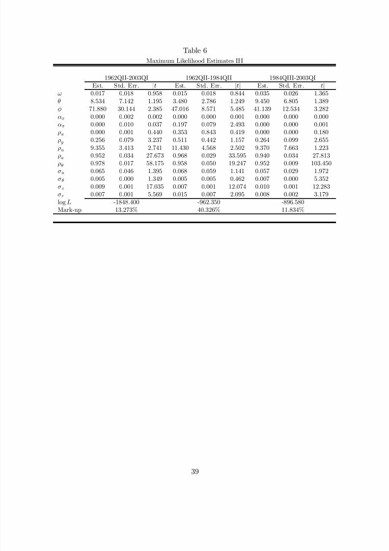
Table 6 of Appendix A presents the estimation results when θ and φ are included in the

list of estimated parameters with a Taylor rule in diff erenced form. The results suggest a

decreasing mark-up from 40% to 12%; however even though a decrease is observed across the

break in the estimate of φ, the pre and post-break estimates are not statistically diff erent

from one another. In addition Table 6 suggests a much larger post-break estimate of ρθ and

σθ than in Tables 4 and 5, which is to be weighed against the fact that the likelihoods of

the model are significantly diff erent, and that the estimate of σθ is still dominated by the

estimate of σz.

Overall, the estimation results suggest that at the very least the influence of the cost-

push shock may be disappearing, which suggests increasingly competitive behavior. Next,

the model estimates suggest, albeit to a much smaller extent, that the role of nominal

rigidities may also be diminishing. Finally, the model estimates suggest a strong role for

demand and technology shocks and that forward-looking behavior may be prevalent in the

data.

Taken as a whole it would seem that, conditional upon the activities of the Bank of

Canada as represented by a Taylor rule, a better characterization of the Canadian economy

may be one that has flexible prices and competitive market structures. Indeed, the model es-

timates presented here along with recent Canadian economic history, summarized above, may

suggest a move towards a real business characterization. Such a transition would not only

imply a change in the sort of shocks that drive the business cycle but perhaps also aggregate

economic policy. This latter contention is clearly simply a supposition and future struc-

30



tural analyses could analyze any implications for policy. Indeed, given parameter instability

and potential identification issues these results should be interpreted as being qualitative in

nature. Planned future Bayesian analyses will specifically address computational issues in

order to provided quantitative evidence of the conjectures presented here.

6 Conclusion

In recent years, high capacity utilization levels have existed without corresponding in-

creases in inflation. In Canada, aggregate capacity utilization rates are based on business

surveys thereby making the Canadian case of high utilization-low inflation of particular

interest. This paper first determined some stylized facts about the relationship in recent

years, namely that there is a break over time in the relationship and that at the very least

utilization has a decreasing eff ect on inflation through time. Given these facts, the conjec-

ture that a move towards increasingly competitive market structures and flexible prices may

have caused a deterioration in the relationship, was explained and evaluated within a New

Keynesian general equilibrium model21.

The conjectures put forth in this paper do not contradict related recent findings. Indeed,

Paquet & Robidoux (2001) find that, in decomposing the Solow residual, an assumption that

the Canadian economy is described by perfect competition and constant returns to scale

best fits the data. In addition, Paquet & Robidoux (2001) find that when capital stocks

are adjusted for capital utilization rates in Canada, productivity shocks are exogenous to

21This break results presented in this paper correspond roughly to the break results reported in Liu &Wong (2003) who test for breaks in the volatility of Canadian output growth. They suggest that betterinventory management may be related to the reduced volatility of GDP growth in Canada. Indeed this lineof argument is relevant here as well and is left for future research.

31



real and monetary forces. The analysis in this paper is complementary to these findings.

Thus, the main contribution of this paper is to first develop stylized facts for a variable that

clearly reflects business conditions due to its’ measurement methodology and then attempt

to explain the facts in a simple, well-known framework.

This paper is also part of an emerging trend in the New Keynesian literature, that of

attempting to model jointly the advantages off ered by ‘efficient’ shocks (that is, shocks to

demand and technology) in New Classical models and the advantages aff orded by recognizing

non-Walrasian features of real world environments, such as those off ered in this paper. Indeed

in the inventive interpretation of the discussion in Clarida, Gali & Gertler (2000), Ireland

(2003) demonstrates that cost-push shocks are as, if not more, important than technology

shocks in explaining the joint behavior of U.S. output, inflation and interest rates. In that

paper, a version of the above model is estimated to demonstrate that the link between New

Keynesian model environments and real business cycle models is slowly disintegrating, and a

new modeling paradigm emerging. The current analysis demonstrates an application of this

new emerging paradigm, an instance in which the Canadian economy may be tending away

from New Keynesian assumptions and towards characterizations provided by real business

cycles.

Finally, when taken as a whole, the results of the present analysis along with those

of Baylor (2001) and Demers (2003), suggest the uncoupling of real resource utilization

from inflation. Several explanations can be off ered for this empirical observation, some of

which were explored formally above. However, in order to fully analyze the causal relations

in the explanations, a more involved analysis is required. In particular, since in Canada

capacity utilization measures are benchmarked to survey data, these survey data may prove

32



useful in sorting through competing explanations behind any breaks in the relationship

between resource utilization and inflation. Thus, irrespective of any formal macroeconomic

evaluation, future research should involve analyzing micro data to uncover underlying causal

relations between changes in capacity utilization and nominal measures of economic activity.

33



References

[1] Alesina, A., Ardagna, S., Nicoletti, G. & Schiantarelli, F. (2003), “Regulation andInvestment”, OECD-ECO Working Paper, No. 352.

[2] Bai, J. & Perron, P. (1998), “Estimating and Testing Linear Models with MultipleStructural Changes”, Econometrica, v. 66.

[3] Baylor, M. (2001), “Capacity Utilization and Inflation: Is Statistics Canada’s Mea-sure an Appropriate Indicator of Inflationary Pressures?”, Department of Finance

Working Paper Series, No. 2001-06.

[4] Corrado, C. & Mattey, J. (1997), “Capacity Utilization”, Journal of Economic Per-

spectives, v. 11.

[5] Clarida, R., Gali, J. & Gertler, M. (2000), “Monetary Policy Rules and MacroeconomicStability: Evidence and Some Theory”, Quarterly Journal of Economics, v. 115.

[6] Demers, F. (2003), “The Canadian Phillips Curve and Regime Shifting”, Bank of

Canada Working Paper Series, No. 03-32.

[7] Emery, K. & Chang, C. (1997), “Is There a Stable Relationship Between CapacityUtilization and Inflation”, Federal Reserve Bank of Dallas Economic Review,First Quarter.

[8] Fagnart, J-F., Licandro, O. & Portier, F. (1999), “Firm Heterogeneity, Capacity Uti-lization and the Business Cycle”, Review of Economic Dynamics, v. 2.

[9] Fillion, J-F. & Leonard, A. (1997), “La Courbe de Phillips au Canada: un examen de

quelques hypothèses”, Bank of Canada Working Paper Series, No. 97-3.

[10] Fixed Capital Flows and Stocks, 1961-1994, Historical , Catalog Number 13-568 XPBStatistics Canada.

[11] Finn, M. G. (1996), “A Theory of the Capacity Utilization/Inflation Relationship”,Federal Reserve Bank of Richmond, Economic Quarterly, v. 82.

[12] Golub, S. (2003), “Measures of Restrictions on Inward Foreign Direct Investment forOECD Countries”, OECD-ECO Working Paper, No. 357.

[13] Gourieroux, C., Monfort, A. & Renault, V (1993), “Indirect Inference”, Journal of

Applied Econometrics, v. 8.

[14] Hamilton, J. D. (1994), Times Series Analysis , Princeton University Press.

[15] Hansen, B. E. (2000), “Sample Splitting and Threshold Estimation”, Econometrica,v. 68.

[16] Ireland, P. (2002), “Endogenous Money or Sticky Prices?”, Journal of Monetary

Economics, forthcoming .

34



[17] Ireland, P. (2003), “Technology Shocks in the New Keynesian Model”, Boston College,mimeo.

[18] Johnson, D. R. (2002), “The Eff ect of Inflation Targeting on the Behavior of ExpectedInflation: Evidence from an 11 Country Panel”, Journal of Monetary Economics,

v. 49.[19] Kim, C-J & Nelson, C. R. (1999), State-Space Models with Regime Switching: Classical

and Gibbs Sampling Approaches with Applications , MIT Press.

[20] Liu, Y. 7 Wong, B-S. (2003), “Estimating Structural Breaks in the Volatility of CanadianOutput Growth", Department of Finance Working Paper Series, No. 2003-20.

[21] Longworth, D. (2002), “Inflation and the Macroeconomy: Changes from the 1980’s tothe 1990’s”, Bank of Canada Review, Spring 2002.

[22] Nicoletti, G. & Scarpetta, S. (2003), “Regulation, Productivity and Growth: OECD

Evidence”, OECD-ECO Working Paper, No. 347.

[23] Paquet, A. & Robidoux, B. (2001), “Issues on the Measurement of the Solow Residualand the Testing of its Exogeneity: Evidence for Canada”, Journal of Monetary

Economics, v. 47.

[24] Rotemberg, J. (1982), “Sticky Prices in the United States”, Journal of Political

Economy, v. 90.

[25] Shapiro, M. D. (1989), “Assessing the Federal Reserve’s Measures of Capacity andUtilization”, Brookings Papers on Economic Activity.

[26] Wen, Y. (1998), “Capacity Utilization Under Increasing Returns to Scale”, Journal of Economic Theory, v. 81.

35



Appendices

A Tables

Table 1Hansen (2000) Estimation Results

Backward Looking Model

1975QI-2002QIV 1975QI-1982QIV 1983QI-2002QIVEst. Std. Err. |t| Est. Std. Err. |t| Est. Std. Err. |t|

α0 -8.418 5.037 1.671 2.329 7.843 0.297 -4.737 4.264 1.111α1 0.108 0.060 1.789 0.066 0.087 0.761 0.069 0.051 1.344α2 0.507 0.119 4.258 0.037 0.157 0.235 0.559 0.120 4.650α3 0.378 0.113 3.356 0.084 0.148 0.564 0.077 0.097 0.792α4 0.021 0.020 1.029 0.034 0.036 0.953 -0.010 0.013 0.760

Obs. 112 32 80R2 0.819 0.034 0.491Break Est.: 1982QIV95% C. I.: 1982QII-1983QI

Mixture Model

1975QI-2002QIV 1975QI-1983QIV 1984QI-2002QIVEst. Std. Err. |t| Est. Std. Err. |t| Est. Std. Err. |t|

α0 -13.185 3.303 3.992 -16.772 4.128 4.063 -7.234 4.591 1.576α1 0.159 0.039 4.032 0.223 0.056 3.974 0.095 0.056 1.680α2 0.058 0.125 0.466 -0.181 0.167 1.084 0.380 0.151 2.521α3 -0.012 0.117 0.103 -0.111 0.131 0.844 -0.046 0.117 0.397

α4 0.899 0.133 6.773 1.069 0.199 5.359 0.391 0.126 3.110α5 0.030 0.016 1.887 0.069 0.027 2.610 -0.006 0.013 0.464Obs. 112 36 76R2 0.877 0.616 0.589Break Est.: 1983QIV95% C. I.: 1982QII-1991QII

36



Table 2

Bai & Perron (1998) Estimation Results

Backward Looking Model Mixture Model

Value 5% Crit. Value 5% Crit.

supF (0|k) Tests 0|1 27.389 18.230 0|1 27.594 20.0800|2 28.945 15.620 0|2 25.730 17.3700|3 34.047 13.930 0|3 30.552 15.5800|4 32.312 12.380 0|4 41.677 13.9000|5 27.737 10.520 0|5 32.983 11.940

Dmax Tests UDmax 34.047 18.420 UDmax 41.677 20.300WDmax 48.065 19.960 WDmax 60.206 21.860

supF (k + 1|k) Tests 2|1 54.603 18.230 2|1 43.140 20.0803|2 39.823 19.910 3|2 35.001 22.1104|3 15.247 20.990 4|3 35.616 23.0405|4 6.404 21.710 5|4 4.890 23.770

Sequential BreaksEst. 95% C. I. Est. 95% C. I.

1st Break 1982QIV 1982QII 1983QII 1983QIV 1982QIV 1984QII2nd Break 1991QI 1990QIII 1991QIII 1997QI 1996QI 1997QII3rd Break .. .. .. 1991QI 1990QIII 1991QIV

Table 3

Kim & Nelson (1999) Estimation Results


Std. Dev. of Est. Std. Err. |t| Std. Dev. of Est. Std. Err. |

t|α0 0.000 0.616 0.000 α0 0.000 0.250 4.687

α1 0.010 0.001 0.001 α1 0.000 0.003 0.000α2 0.232 0.035 6.900 α2 0.083 0.040 0.000α3 0.000 0.028 6.631 α3 0.000 0.019 2.067α4 0.006 0.004 0.000 α4 0.177 0.037 0.000σ 0.000 0.365 1.587 α5 0.005 0.004 4.747

σ 0.521 0.111 1.223logL -179.680 logL -159.680R2 0.666 LM 26.012 R2 0.767 LM 9.322

37



Table 4

Maximum Likelihood Estimates I

1962QII-2003QI 1962QII-1984QII 1984QIII-2003QIEst. Std. Err. |t| Est. Std. Err. |t| Est. Std. Err. |t|

ω 0.013 0.008 1.759 0.014 0.009 1.606 0.035 0.011 3.238αx 0.000 0.000 0.000 0.000 0.000 0.000 0.000 0.000 0.000απ 0.000 0.000 0.000 0.000 0.000 0.000 0.085 0.070 1.206ρr 1.032 0.037 28.241 1.020 0.031 32.667 0.939 0.017 55.817ρπ 0.000 0.002 0.000 0.000 0.003 0.000 0.051 0.042 1.213ρg 0.288 0.120 2.406 0.307 0.158 1.943 0.000 0.000 0.000

ρu 14.151 11.736 1.206 13.961 12.200 1.144 5.059 1.073 4.715ρa 0.970 0.017 55.571 0.975 0.018 54.212 0.979 0.003 378.050ρe 0.974 0.016 60.672 0.956 0.030 31.390 0.080 0.105 0.763σa 0.108 0.059 1.843 0.132 0.089 1.488 0.060 0.009 6.786σe 0.006 0.003 2.163 0.009 0.005 1.608 0.003 0.001 2.485σz 0 .009 0.000 17.679 0.010 0.001 12.976 0.007 0.001 11.703σr 0.008 0.003 2.721 0.009 0.004 2.319 0.007 0.001 11.927

logL -1907.200 -1010.100 -902.970

Table 5

Maximum Likelihood Estimates II


ω 0.012 0.008 1.511 0.017 0.015 1.168 0.000 0.000 0.000ψ 6.752 4.515 1.496 8.229 5.516 1.492 0.002 0.001 1.778αx 0.000 0.000 0.000 0.000 0.000 0.000 0.725 0.146 4.961απ 0.000 0.000 0.000 0.000 0.000 0.000 0.003 0.097 0.030ρr 1 .028 0.025 41.380 1.025 0.041 24.850 0.980 0.024 40.409ρπ 0.000 0.000 0.000 0.000 0.003 0.000 0.102 0.046 2.228ρg 0.289 0.089 3.224 0.308 0.176 1.754 0.231 0.072 3.188

ρu 12.282 11.114 1.105 17.305 15.058 1.149 0.000 0.000 0.001ρa 0.971 0.004 260.130 0.972 0.017 56.679 0.979 0.016 62.041ρe 0.974 0.011 90.531 0.956 0.021 44.885 0.000 0.000 0.000σa 0.114 0.013 8.775 0.121 0.067 1.803 0.096 0.068 1.400σe 0.000 0.000 3.954 0.000 0.000 2.476 0.005 0.001 7.829σz 0.009 0.001 16.608 0.010 0.001 13.002 0.004 0.001 3.048σr 0.008 0.003 2.841 0.010 0.004 2.609 0.002 0.000 7.267

logL -1907.200 -1010.100 -929.760

38



Table 6

Maximum Likelihood Estimates III


ω 0.017 0.018 0.958 0.015 0.018 0.844 0.035 0.026 1.365θ 8.534 7.142 1.195 3.480 2.786 1.249 9.450 6.805 1.389φ 71.880 30.144 2.385 47.016 8.571 5.485 41.139 12.534 3.282αx 0.000 0.002 0.002 0.000 0.000 0.001 0.000 0.000 0.000απ 0.000 0.010 0.037 0.197 0.079 2.493 0.000 0.000 0.001ρπ 0.000 0.001 0.440 0.353 0.843 0.419 0.000 0.000 0.180ρg 0.256 0.079 3.237 0.511 0.442 1.157 0.264 0.099 2.655

ρu 9.355 3.413 2.741 11.430 4.568 2.502 9.370 7.663 1.223ρa 0.952 0.034 27.673 0.968 0.029 33.595 0.940 0.034 27.813ρθ 0.978 0.017 58.175 0.958 0.050 19.247 0.952 0.009 103.450σa 0.065 0.046 1.395 0.068 0.059 1.141 0.057 0.029 1.972σθ 0.005 0.000 1.349 0.005 0.005 0.462 0.007 0.000 5.352σz 0.009 0.001 17.035 0.007 0.001 12.074 0.010 0.001 12.283

σr 0.007 0.001 5.569 0.015 0.007 2.095 0.008 0.002 3.179logL -1848.400 -962.350 -896.580Mark-up 13.273% 40.326% 11.834%

39



B Figures

Figure 1

1975QI-2002QIV

0%

2%

4%

6%

8%

10%

12%

14%

1975QI 1978QI 1981QI 1984QI 1987QI 1990QI 1993QI 1996QI 1999QI 2002QI

70%

72%

74%

76%

78%

80%

82%

84%

86%

88%

Core CPI Inflation (Left Axis) Capacity Utilization

40



Figure 2

1975QI-2002QIV

-7%

-6%

-5%

-4%

-3%

-2%

-1%

0%

1%

2%

3%

1975QI 1978QI 1981QI 1984QI 1987QI 1990QI 1993QI 1996QI 1999QI 2002QI

70%

72%

74%

76%

78%

80%

82%

84%

86%

88%

Output Gap (Left Axis) Capacity Utilization

41



Figure 4

Estimated Time Varying Coefficient on Capacity Utilization (α1t)

0.00

0.10

0.20

0.30

0.40

0.50

0.60

0.70

0.80

0.90

1.00

1978QI 1981QI 1984QI 1987QI 1990QI 1993QI 1996QI 1999QI 2002QI


43



Figure 5

Conditional Variances

0.00

2.00

4.00

6.00

8.00

10.00

12.00

14.00

16.00



44



Figure 6

Forecast Errors

-10.00

-8.00

-6.00

-4.00

-2.00

0.00

2.00

4.00

6.00

8.00

10.00

