Why Simple Hash Functions Work:

Exploiting the Entropy in a Data Stream∗

Michael Mitzenmacher† Salil Vadhan‡

School of Engineering & Applied SciencesHarvard University

Cambridge, MA 02138michaelm,salil@eecs.harvard.edu

http://eecs.harvard.edu/∼michaelm,salilOctober 12, 2007

Abstract

Hashing is fundamental to many algorithms and data structures widely used in practice. Fortheoretical analysis of hashing, there have been two main approaches. First, one can assumethat the hash function is truly random, mapping each data item independently and uniformlyto the range. This idealized model is unrealistic because a truly random hash function requiresan exponential number of bits to describe. Alternatively, one can provide rigorous bounds onperformance when explicit families of hash functions are used, such as 2-universal or O(1)-wiseindependent families. For such families, performance guarantees are often noticeably weakerthan for ideal hashing.

In practice, however, it is commonly observed that simple hash functions, including 2-universal hash functions, perform as predicted by the idealized analysis for truly random hashfunctions. In this paper, we try to explain this phenomenon. We demonstrate that the strongperformance of universal hash functions in practice can arise naturally from a combination ofthe randomness of the hash function and the data. Specifically, following the large body ofliterature on random sources and randomness extraction, we model the data as coming from a“block source,” whereby each new data item has some “entropy” given the previous ones. Aslong as the (Renyi) entropy per data item is sufficiently large, it turns out that the performancewhen choosing a hash function from a 2-universal family is essentially the same as for a trulyrandom hash function. We describe results for several sample applications, including linearprobing, balanced allocations, and Bloom filters.

Keywords: Hashing, Pairwise Independence, Bloom Filters, Linear Probing, Balanced Allo-cations, Randomness Extractors.

∗A preliminary version of this paper will appear in SODA 2008.†Supported by NSF grant CCF-0634923 and grants from Yahoo! Inc. and Cisco, Inc.‡Work done in part while visiting U.C. Berkeley. Supported by ONR grant N00014-04-1-0478, NSF grant CCF-

0133096, US-Israel BSF grant 2002246, a Guggenheim Fellowship, and the Miller Institute for Basic Research inScience.

Contents

1 Introduction 2

2 Preliminaries 4

3 Hashing Worst-Case Data 53.1 Linear Probing . . . . . . . . . . . . . . . . . . . . . . . . . . . . . . . . . . . . . . . 53.2 Balanced Allocations. . . . . . . . . . . . . . . . . . . . . . . . . . . . . . . . . . . . 53.3 Bloom Filters . . . . . . . . . . . . . . . . . . . . . . . . . . . . . . . . . . . . . . . . 6

4 Hashing Block Sources 94.1 Random Sources . . . . . . . . . . . . . . . . . . . . . . . . . . . . . . . . . . . . . . 94.2 Extracting Randomness . . . . . . . . . . . . . . . . . . . . . . . . . . . . . . . . . . 104.3 Optimized Block-Source Extraction . . . . . . . . . . . . . . . . . . . . . . . . . . . . 12

5 Applications 155.1 Linear Probing . . . . . . . . . . . . . . . . . . . . . . . . . . . . . . . . . . . . . . . 155.2 Balanced Allocations . . . . . . . . . . . . . . . . . . . . . . . . . . . . . . . . . . . . 165.3 Bloom Filters . . . . . . . . . . . . . . . . . . . . . . . . . . . . . . . . . . . . . . . . 17

6 Alternative Approaches 18

7 Conclusion 19

1

1 Introduction

Hashing is at the core of many fundamental algorithms and data structures, including all varietiesof hash tables [Knu], Bloom filters and their many variants [BM2], summary algorithms for datastreams [Mut], and many others. Traditionally, applications of hashing are analyzed as if the hashfunction is a truly random function (a.k.a. “random oracle”) mapping each data item independentlyand uniformly to the range of the hash function. However, this idealized model is unrealistic,because a truly random function mapping 0, 1n to 0, 1m requires an exponential number of bitsto describe.

For this reason, a line of theoretical work, starting with the seminal paper of Carter and Weg-man [CW] on universal hashing, has sought to provide rigorous bounds on performance whenexplicit families of hash functions are used, e.g. ones whose description and computational com-plexity are polynomial in n and m. While many beautiful results of this type have been obtained,they are not always as strong as we would like. In some cases, the types of hash functions analyzedcan be implemented very efficiently (e.g. universal or O(1)-wise independent), but the performanceguarantees are noticeably weaker than for ideal hashing. (A motivating recent example is theanalysis of linear probing under 5-wise independence [PPR].) In other cases, the performance guar-antees are (essentially) optimal, but the hash functions are more complex and expensive (e.g. witha super-linear time or space requirement). For example, if at most T items are going to be hashed,then a T -wise independent hash function will have precisely the same behavior as an ideal hashfunction. But a T -wise independent hash function mapping to 0, 1m requires at least T ·m bits torepresent, which is often too large. For some applications, it has been shown that less independence,such as O(log T )-wise independence, suffices, e.g. [SS, PR], but such functions are still substantiallyless efficient than 2-universal hash functions. A series of works [Sie, OP, DW] have improved thetime complexity of (almost) T -wise independence to a constant number of word operations, but thespace complexity necessarily remains at least T ·m.

In practice, however, the performance of standard universal hashing seems to match what ispredicted for ideal hashing. This phenomenon was experimentally observed long ago in the settingof Bloom filters [Ram2]; other reported examples include [BM1, DKSL, PR, Ram1, RFB]. Thus,it does not seem truly necessary to use the more complex hash functions for which this kind ofperformance can be proven. We view this as a significant gap between the theory and practice ofhashing.

In this paper, we aim to bridge this gap. Specifically, we suggest that it is due to the use ofworst-case analysis. Indeed, in some cases, it can be proven that there exist sequences of dataitems for which universal hashing does not provide optimal performance. But these bad sequencesmay be pathological cases that are unlikely to arise in practice. That is, the strong performance ofuniversal hash functions in practice may arise from a combination of the randomness of the hashfunction and the randomness of the data.

Of course, doing an average-case analysis, whereby each data item is independently and uni-formly distributed in 0, 1n, is also very unrealistic (not to mention that it trivializes many ap-plications). Here we propose that an intermediate model, previously studied in the literature onrandomness extraction [CG], may be an appropriate data model for hashing applications. Underthe assumption that the data fits this model, we show that relatively weak hash functions achieveessentially the same performance as ideal hash functions.

2

Our Model. We model the data as coming from a random source in which the data items can befar from uniform and have arbitrary correlations, provided that each (new) data item is sufficientlyunpredictable given the previous items. This is formalized by Chor and Goldreich’s notion of ablock source [CG],1 where we require that the i’th item Xi has at least some k bits of “entropy”conditioned on the previous items X1, . . . , Xi−1. There are various choices for the entropy measurethat can be used here; Chor and Goldreich use min-entropy, but most of our results hold even forthe less stringent measure of Renyi entropy.

Our work is very much in the same spirit as previous works that have examined intermediatemodels between worst-case and average-case analysis of algorithms for other kinds of problems.Examples include the semi-random graph model of Blum and Spencer [BS], and the smoothedanalysis of Spielman and Teng [ST]. Interestingly, Blum and Spencer’s semi-random graph modelsare based on Santha and Vazirani’s model of semi-random sources [SV], which in turn were theprecursor to the Chor–Goldreich model of block sources [CG]. Chor and Goldreich suggest usingblock sources as an input model for communication complexity, but surprisingly it seems that noone has considered them as an input model for hashing applications.

Our Results. Our first observation is that standard results in the literature on randomnessextractors already imply that universal hashing performs nearly as well ideal hashing, provided thedata items have enough entropy [BBR, ILL, CG, Zuc]. Specifically, if we have T data items comingfrom a block source (X1, . . . , XT ) where each data item has (Renyi) entropy at least m+2 log(T/ε)and H is a random universal hash function mapping to 0, 1m, then (H(X1), . . . ,H(XT )) hasstatistical difference at most ε from T uniform and independent elements of 0, 1m. Thus, anyevent that would occur with some probability p under ideal hashing now occurs with probabilityp ± ε. This allows us to automatically translate existing results for ideal hashing into results foruniversal hashing in our model.

In our remaining results, we focus on reducing the amount of entropy required from the dataitems. Assuming our hash function has a description size o(mt), then we must have (1 − o(1))mbits of entropy per item for the hashing to “behave like” ideal hashing (because the entropy of(H(X1), . . . , H(XT )) is at most the sum of the entropies of H and the Xi’s). The standard analysismentioned above requires an additional 2 log(T/ε) bits of entropy per block. In the randomnessextraction literature, the additional entropy required is typically not significant because log(T/ε)is much smaller than m. However, it can be significant in our applications. For example, a typicalsetting is hashing T = Θ(M) items into 2m = M bins. Here m + 2 log(T/ε) ≥ 3m−O(1) and thusthe standard analysis requires 3 times more entropy than the lower bound of (1 − o(1))m. (Thebounds obtained for the specific applications mentioned below are even larger, sometimes due tothe need for a subconstant ε and sometimes due to the fact items need to be hashed into severallocations.)

We use a variety of general techniques to reduce the entropy required. These include switchingfrom statistical difference (equivalently, `1 distance) to Renyi entropy (equivalently, `2 distance orcollision probability) throughout the analysis and decoupling the probability that a hash functionis “good” from the uniformity of the hashed values h(Xi). We can reduce the entropy required evenfurther if we use 4-wise independent hash functions, which also have very fast implementations [TZ].

1Chor and Goldreich called these probability-bounded sources, but the term block source has become more commonin the literature.

3

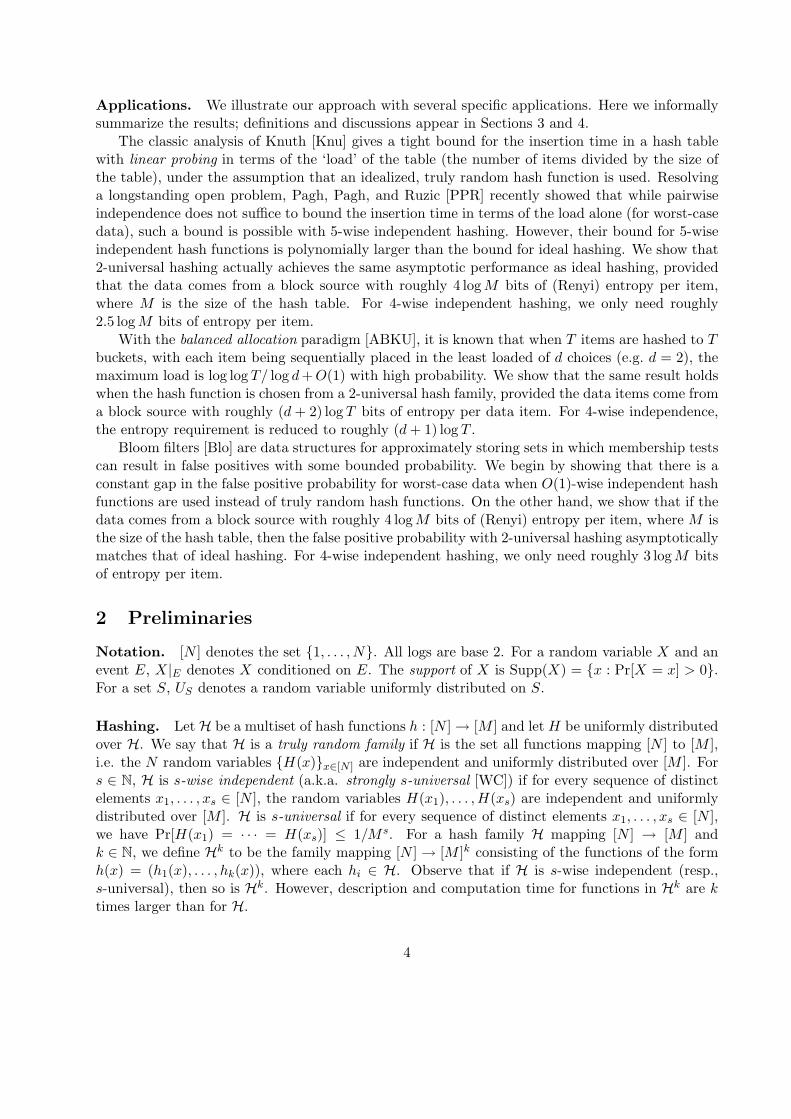
Applications. We illustrate our approach with several specific applications. Here we informallysummarize the results; definitions and discussions appear in Sections 3 and 4.

The classic analysis of Knuth [Knu] gives a tight bound for the insertion time in a hash tablewith linear probing in terms of the ‘load’ of the table (the number of items divided by the size ofthe table), under the assumption that an idealized, truly random hash function is used. Resolvinga longstanding open problem, Pagh, Pagh, and Ruzic [PPR] recently showed that while pairwiseindependence does not suffice to bound the insertion time in terms of the load alone (for worst-casedata), such a bound is possible with 5-wise independent hashing. However, their bound for 5-wiseindependent hash functions is polynomially larger than the bound for ideal hashing. We show that2-universal hashing actually achieves the same asymptotic performance as ideal hashing, providedthat the data comes from a block source with roughly 4 log M bits of (Renyi) entropy per item,where M is the size of the hash table. For 4-wise independent hashing, we only need roughly2.5 log M bits of entropy per item.

With the balanced allocation paradigm [ABKU], it is known that when T items are hashed to Tbuckets, with each item being sequentially placed in the least loaded of d choices (e.g. d = 2), themaximum load is log log T/ log d + O(1) with high probability. We show that the same result holdswhen the hash function is chosen from a 2-universal hash family, provided the data items come froma block source with roughly (d + 2) log T bits of entropy per data item. For 4-wise independence,the entropy requirement is reduced to roughly (d + 1) log T .

Bloom filters [Blo] are data structures for approximately storing sets in which membership testscan result in false positives with some bounded probability. We begin by showing that there is aconstant gap in the false positive probability for worst-case data when O(1)-wise independent hashfunctions are used instead of truly random hash functions. On the other hand, we show that if thedata comes from a block source with roughly 4 log M bits of (Renyi) entropy per item, where M isthe size of the hash table, then the false positive probability with 2-universal hashing asymptoticallymatches that of ideal hashing. For 4-wise independent hashing, we only need roughly 3 logM bitsof entropy per item.

2 Preliminaries

Notation. [N ] denotes the set 1, . . . , N. All logs are base 2. For a random variable X and anevent E, X|E denotes X conditioned on E. The support of X is Supp(X) = x : Pr[X = x] > 0.For a set S, US denotes a random variable uniformly distributed on S.

Hashing. Let H be a multiset of hash functions h : [N ] → [M ] and let H be uniformly distributedover H. We say that H is a truly random family if H is the set all functions mapping [N ] to [M ],i.e. the N random variables H(x)x∈[N ] are independent and uniformly distributed over [M ]. Fors ∈ N, H is s-wise independent (a.k.a. strongly s-universal [WC]) if for every sequence of distinctelements x1, . . . , xs ∈ [N ], the random variables H(x1), . . . ,H(xs) are independent and uniformlydistributed over [M ]. H is s-universal if for every sequence of distinct elements x1, . . . , xs ∈ [N ],we have Pr[H(x1) = · · · = H(xs)] ≤ 1/Ms. For a hash family H mapping [N ] → [M ] andk ∈ N, we define Hk to be the family mapping [N ] → [M ]k consisting of the functions of the formh(x) = (h1(x), . . . , hk(x)), where each hi ∈ H. Observe that if H is s-wise independent (resp.,s-universal), then so is Hk. However, description and computation time for functions in Hk are ktimes larger than for H.

4

3 Hashing Worst-Case Data

In this section, we describe the three main hashing applications we study in this paper — linearprobing, balanced allocations, and Bloom filters — and describe mostly known results about whatcan be achieved for worst-case data. Here and throughout the paper, where appropriate we leaveproofs to the appendix because of space.

3.1 Linear Probing

A hash table using linear probing stores a sequence x = (x1, . . . , xT ) of data items from [N ] usingM memory locations. Given a hash function h : [N ] → [M ], we place the elements x1, . . . , xT

sequentially as follows. The element xi first attempts placement at h(xi), and if this location isalready filled, locations h(xi) + 1 mod M , h(xi) + 2 mod M , and so on are tried until an emptylocation is found. The ratio α = T/M is referred to as the load of the table. The efficiency of linearprobing is measured according to the insertion time for a new data item. (Other measures, suchas the average time to search for items already in the table, are also often studied, and our resultscan be generalized to these measures as well.)

Definition 3.1 Given h : [N ] → [M ], a sequence x = (x1, . . . , xT ) of data items from [N ] storedvia linear probing using h, we define the insertion time TimeLP(x, h) to be the value of j such thatxT is placed at location h(xi) + (j − 1) mod M .

It is well known that with ideal hashing, the expected time can be bounded quite tightly as afunction of the load [Knu].

Theorem 3.2 ([Knu]) Let H be a truly random hash function mapping [N ] to [M ]. For everysequence x ∈ [N ]T , we have E[TimeLP(x,H)] ≤ 1/(1− α)2, where α = T/M is the load.

Resolving a longstanding open problem, Pagh, Pagh, and Ruzic [PPR] recently showed thatthe expected lookup time could be bounded in terms of α using only O(1)-wise independence.Specifically, with 5-wise independence, the expected time for an insertion is O

(1

(1−α)3

)for any

sequence x. On the other hand, in [PPR] it is also shown that there are examples of sequences xand pairwise independent hash families such that the expected time for a lookup is logarithmic inT (even though the load α is independent of T ). In contrast, our work demonstrates that pairwiseindependent hash functions yield expected lookup times that are asymptotically the same as underthe idealized analysis, assuming there is sufficient entropy in the data items themselves.

3.2 Balanced Allocations.

A hash table using the balanced allocation paradigm [ABKU] with d ∈ N choices stores a sequencex = (x1, . . . , xT ) ∈ [N ]T in an array of M buckets. Let h be a hash function mapping [N ] to[M ]d ∼= [Md], where we view the components of h(x) as (h1(x), . . . , hd(x)). We place the elementssequentially by putting xi in the least loaded of the d buckets h1(xi), . . . , hd(xi) at time i (breakingties arbitrarily), where the load of a bucket at time i is the number elements from x1, . . . , xi−1

placed in it.

5

Definition 3.3 Given h : [N ] → [M ]d, a sequence x = (x1, . . . , xT ) of data items from [N ]stored via the balanced allocation paradigm (with d choices) using h, we define the maximum loadMaxLoadBA(x, h) to be the maximum load of among the buckets at time T + 1.

In the case that the number T of items is the same as the number M of buckets and we dobalanced allocation with d = 1 choice (i.e. standard load balancing), it is known that the maximumload is Θ(log T/ log log T ) with high probability. Remarkably, when the number of choices d is twoor larger, the maximum load drops to be double-logarithmic.

Theorem 3.4 ([ABKU, Voc]) For every d ≥ 2 and γ > 0, there is a constant c such the fol-lowing holds. Let H be a truly random hash function mapping [N ] to [T ]d. For every sequencex ∈ [N ]T of distinct data items, we have

Pr[MaxLoadBA(x,H) >log log T

log d+ c] ≤ 1

T γ.

There are other variations on this scheme, including the asymmetric version due to Vocking[Voc] and cuckoo hashing [PR]; we choose to study the original setting for simplicity.

The asymmetric scheme has been recently studied under explicit functions [Woe], similar tothose of [DW]. At this point, we know of no non-trivial upper or lower bounds for the balancedallocation paradigm using families of hash functions with constant independence, although perfor-mance has been tested empirically [BM1]. Such bounds have been a long-standing open questionin this area.

3.3 Bloom Filters

A Bloom filter [Blo] represents a set x = x1, . . . , xT where each xi ∈ [N ] using an array of Mbits and ` hash functions. For our purposes, it will be somewhat easier to work with a segmentedBloom filter, where the M bits are partitioned into ` disjoint subarrays of size M/`, with onesubarray for each hash function. We assume that M/` is an integer. (This splitting does notsubstantially change the results from the standard approach of having all hash functions map intoa single array of size M .) As in the previous section, we denote the components of a hash functionh : [N ] → [M/`]` ∼= [(M/`)`], as providing ` hash values h(x) = (h1(x), . . . , h`(x)) ∈ [M/`]` in thenatural way. The Bloom filter is initialized by setting all bits to 0, and then setting the hi(xj)’th bitto be 1 in the i’th subarray for all i ∈ [`] and j ∈ [T ]. Given an element y, one tests for membershipin x by accepting if the hi(y)’th bit is 1 in the i’th subarray for all i ∈ [`], and rejecting otherwise.Clearly, if y ∈ x, then the algorithm will always accept. However, the algorithm may err if y /∈ x.

Definition 3.5 Given h : [N ] → [M/`]` (where ` divides M), a sequence x = (x1, . . . , xT ) of dataitems from [N ] stored in an `-segment Bloom filter using h, and an additional element y ∈ [N ],we define the false positive predicate FalsePosBF(h, x, y) to be 1 if y 6∈ x and the membership testaccepts. That is, if y /∈ x yet hi(y) ∈ hi(x) def= hi(xj) : j = 1, . . . , T for all i = 1, . . . , `.

For truly random families of hash functions, it is easy to compute the false positive probability.

Theorem 3.6 ([Blo]) Let H be a truly random hash function mapping [N ] to [M/`]` (where `divides M). For every sequence x ∈ [N ]T of data items and every y /∈ x, we have

Pr[FalsePosBF(H, x, y) = 1] =

(1−

(1− `

M

)T)`

≈(1− e−`T/M

)`.

6

In the typical case that M = Θ(T ), the asymptotically optimal number of hash functions is` = (M/T ) · ln 2, and the false positive probability is approximately 2−`.

Below we will describe the kinds of results that can be proven about Bloom filters on worst-casedata using O(1)-wise independence. But the following more mild reduction in randomness, using 2truly random hash functions instead of `, will be useful later.

Theorem 3.7 ([KM]) Let H = (H1,H2) be a truly random hash function mapping [N ] to [M/`]2,where M/` is a prime integer. Define H ′ = (H ′

1, . . . , H′`) : [N ] → [M/`]` by H ′

i(w) = H1(w) + (i−1)H2(w) mod M/`. Then for every sequence x ∈ [N ]T of T data items and every y /∈ x, we have

Pr[FalsePosBF(H ′, x, y) = 1] ≤(

1−(

1− `

M

)T)`

+ O(1/M).

The restriction to prime integers M/` is not strictly necessary in general; for more complete state-ments of when 2 truly random hash functions suffice, see [KM].

We now turn to the worst-case performance of Bloom filters under O(1)-wise independence. Itis folklore that 2-universal hash functions can be used with a constant-factor loss in space efficiency.Indeed, a union bound shows that Pr[hi(y) ∈ hi(x)] is at most T ·(`/M), compared to 1−(1−`/M)T

in the case of truly random hash functions. This can be generalized to s-wise independent familiesusing the following inclusion-exclusion formula.

Lemma 3.8 Let H : [N ] → [M/`] be a hash function chosen at random from a family H (where`|M). For every sequence x ∈ [N ]T , every y /∈ x, and every even s ≤ T , we have

Pr[H(y) ∈ H(x)] =T∑

j=1

(−1)j+1∑

U⊆T,|U |=j

Pr[H(y) = H(w) ∀w ∈ U ].

≤s−1∑

j=1

(−1)j+1∑

U⊆T,|U |=j

Pr[H(y) = H(w) ∀w ∈ U ]

If H is an s-universal hash family, then the first s − 1 terms of the outer sum above are thesame as for a truly random function (namely (−1)j+1 ·(T

j

)(`/M)j). This gives the following bound.

Proposition 3.9 Let s be an even constant. Let H be an s-universal family mapping [N ] to [M/`](where ` divides M), and let H = (H1, . . . ,H`) be a random hash function from H`. For everysequence x ∈ [N ]T of T ≤ M/` data items and every y /∈ x, we have

Pr[FalsePosBF(H,x, y) = 1] ≤(

1−(

1− `

M

)T

+ O

(`T

M

)s)`

.

Proof: By Lemma 3.8, for each i = 1, . . . , `, we have:

Pr[Hi(y) ∈ Hi(x)] ≤ −s−1∑

j=1

(−1)j∑

U⊆T,|U |=j

Pr[Hi(y) = Hi(w) ∀w ∈ U ]

7

= −s−1∑

j=1

(−1)j ·(

T

j

)(`

M

)j

(by s-universality)

= −

(1− `

M

)T

− 1−T∑

j=s

(−1)j ·(

T

j

)(`

M

)j

≤ 1−(

1− `

M

)T

+ O

(`T

M

)s

Thus,

Pr[FalsePosBF(H, x, y) = 1] = Pr[Hi(y) ∈ Hi(x) ∀i] ≤(

1−(

1− `

M

)T

+ O

(`T

M

)s)`

.

Notice that in the common case that ` = Θ(1) and M = Θ(T ), so that the false positiveprobability is constant, the above bound differs from the one for ideal hashing by an amount thatshrinks rapidly with s. However, when s is constant, the difference remains an additive constant.Another way of interpreting this is that to obtain a given guarantee on the false positive probabilityusing O(1)-wise independence instead of ideal hashing, one must pay a constant factor in the spacefor the Bloom filter. The following proposition shows that this loss is necessary if we use onlyO(1)-wise independence.

Proposition 3.10 Let s be an even constant. For all N, M, `, T ∈ N such that M/` is a primepower and T < minM/`,N, there exists an (s + 1)-wise independent family of hash functionsH mapping [N ] to [M/`] a sequence x ∈ [N ]T of data items, and a y ∈ [N ] \ x, such that ifH = (H1, . . . , H`) is a random hash function from H`, we have

Pr[FalsePosBF(H, x, y) = 1] ≥(

1−(

1− `

M

)T

− Ω(

`T

M

)s)`

.

Proof: Let q = M/`, and let F be the finite field of size q. Associate the elements of [M/`] withelements of F, and similarly for the first M/` elements of [N ]. Let H1 consist of all polynomialsf : F→ F of degree at most s− 1; this is an (s + 1)-wise independent family. Let H2 consist of any(s + 1)-wise independent family mapping [N ] \ F to F. For a function f ∈ H1 and g ∈ H2, defineh = f ∪ g : [N ] → [M/`] by h(x) = f(x) if x ∈ F and h(x) = g(x) if x /∈ F. Let H be the multisetof all such functions f ∪ g. We let x be an arbitrary sequence of T − 1 distinct elements of F, andy any other element of F.

Again we compute the false positive probability using Lemma 3.8. The first s terms can becomputed exactly as before, using (s + 1)-universality. For the terms beyond s, we observe thatwhen |U | ≥ s, it is the case that hi(y) = hi(w) for all w ∈ U if and only if hi = f ∪ g for a constantpolynomial f . The reason is that no nonconstant polynomial of degree at most s can take on thesame value more than s times. The probability that a random polynomial of degree at most s is aconstant polynomial is 1/qs = (`/M)s.

8

Pr[Hi(y) ∈ Hi(x)] =T∑

j=1

(−1)j+1∑

U⊆T,|U |=j

Pr[Hi(y) = Hi(w) ∀w ∈ U ]

=

s−1∑

j=1

(−1)j+1 ·(

T

j

)(`

M

)j +

T∑

j=s

(−1)j+1 ·(

T

j

)(`

M

)s

=

1−

(1− `

M

)T

+T∑

j=s

(−1)j ·(

T

j

)(`

M

)j +

s−1∑

j=0

(−1)j ·(

T

j

) (`

M

)s

≥[1−

(1− `

M

)T

+ Ω(

`T

M

)s]−O

(T s−1 ·

(`

M

)s)

= 1−(

1− `

M

)T

+ Ω(

`T

M

)s

Again, to bound the false positive probability, we simply raise the above to the `’th power.

4 Hashing Block Sources

4.1 Random Sources

We view our data items as being random variables distributed over a finite set of size N , whichwe identify with [N ]. We use the following quantities to measure the amount of randomness ina data item. For a random variable X, the max probability of X is mp(X) = maxx Pr[X = x].The collision probability of X is cp(X) =

∑x Pr[X = x]2. Measuring these quantities is equivalent

to measuring the min-entropy H∞(X) = minx log(1/Pr[X = x]) = log(1/mp(X)) and the Renyientropy H2(X) = log(1/Ex←X [Pr[X = x]]) = log(1/cp(X)). If X is supported on a set of size K,then mp(X) ≥ cp(X) ≥ 1/K (i.e. H∞(X) ≤ H2(X) ≤ log K), with equality iff X is uniform onits support. It also holds that mp(X) ≤ cp(X)1/2 (i.e. H∞(X) ≥ H2(X)/2), so min-entropy andRenyi entropy are always within a factor of 2 of each other.

We model a sequence of data items as a sequence (X1, . . . , XT ) of correlated random variableswhere each item is guaranteed to have some entropy even conditioned on the previous items.

Definition 4.1 A sequence of random variables (X1, . . . , XT ) taking values in [N ]T is a blocksource with collision probability p per block (respectively, max probability p per block) if for everyi ∈ [T ] and every (x1, . . . , xi−1) ∈ Supp(X1, . . . , Xi−1), we have cp(Xi|X1=x1,...,Xi−1=xi−1) ≤ p(respectively, mp(Xi|X1=x1,...,Xi−1=xi−1) ≤ p

When max probability is used as the measure of entropy, then this is precisely the model ofsources suggested by Chor and Goldreich [CG] in the literature on randomness extractors. We willmainly use the collision probability formulation as the entropy measure, since it makes our resultsmore general.

A useful fact is that collision/max probability of the entire sequence is at most the product ofthe collision/max probabilities contributed by the blocks.

9

Lemma 4.2 If a sequence of random variables Y = (Y1, . . . , YT ) taking values in [N ]T has collisionprobability 1/N + 1/K per block, then cp(Y ) ≤ (1/N + 1/K)T .

Proof: By induction on T . The base case T = 0 follows by definition. For T > 0, let Y ′ =(Y ′

1 , . . . , Y′T ) be an iid copy of Y . Let Z be the distribution of (Y1, . . . , YT−1) conditioned on

(Y1, . . . , YT−1) = (Y ′1 , . . . , Y

′T−1).

cp(Y ) = Pr[Y = Y ′]= Pr[(Y1, . . . , YT−1) = (Y ′

1 , . . . , Y′T−1)] · Pr[YT = Y ′

T |(Y1, . . . , YT−1) = (Y ′1 , . . . , Y

′T−1)]

= cp(Y1, . . . , YT−1) · E(y1,...,yT−1)←Z

[Pr[YT = Y ′T |Y1 = Y ′

1 = y1, . . . , YT−1 = Y ′T−1 = yT−1]]

= cp(Y1, . . . , YT−1) · E(y1,...,yT−1)←Z

[cp(YT |Y1 = y1, . . . , YT−1 = yT−1)]

≤ (1/N + 1/K)T−1 · (1/N + 1/K).

Another useful fact is that we can bound the collision probability of a random variable in termsof conditioned versions of that variable.

Lemma 4.3 Let (X,Y ) be jointly distributed random variables. Then cp(X) ≤ maxy∈Supp(Y ) cp(X|Y =y).

Proof: Then

cp(X) =∑

x

Pr[X = x]2

=∑

x

(∑

y

Pr[Y = y] · Pr[X = x|Y = y]) · (∑

y′Pr[Y = y′] · Pr[X = x|Y = y′])

=∑

y,y′Pr[Y = y] · Pr[Y = y′] ·

∑x

Pr[X = x|Y = y] · Pr[X = x|Y = y′]

≤∑

y,y′Pr[Y = y] · Pr[Y = y′] ·

(∑x

Pr[X = x|Y = y]2)1/2

·(∑

x

Pr[X = x|Y = y′]2)1/2

=∑

y,y′Pr[Y = y] · Pr[Y = y′] · cp(X|Y = y)1/2 · cp(X|Y = y′)1/2

≤ maxy∈Supp(Y )

cp(X|Y = y)

4.2 Extracting Randomness

A randomness extractor [NZ] can be viewed as a family of hash functions with the property that forany random variable X with enough entropy, if we pick a random hash function h from the family,then h(X) is “close” to being uniformly distributed on the range of the hash function. Randomnessextractors are a central object in the theory of pseudorandomness and have many applications in

10

theoretical computer science. Thus there is a large body of work on the construction of randomnessextractors. (See the surveys [NT, Sha]). A major emphasis in this line of work is constructingextractors where it takes extremely few (e.g. a logarithmic number of) random bits to choose ahash function from the family. This parameter is less crucial for us, so instead our emphasis is onusing simple and very efficient hash functions (e.g. universal hash functions) and minimizing theamount of entropy needed from the source X. To do this, we will measure the quality of a hashfamily in ways that are tailored to our application, and thus we do not necessarily work with thestandard definitions of extractors.

In requiring that the hashed value h(X) be ‘close’ to uniform, the standard definition of anextractor uses the most natural measure of ‘closeness’. Specifically, for random variables X andY , taking values in [N ], their statistical difference is defined as ∆(X, Y ) = maxS⊆[N ] |Pr[X ∈S]− Pr[Y ∈ S]|. X and Y are called ε-close if ∆(X, Y ) ≤ ε.

The classic Leftover Hash Lemma shows that universal hash functions are randomnness extrac-tors with respect to statistical difference.

Lemma 4.4 (The Leftover Hash Lemma [BBR, ILL]) Let H : [N ] → [M ] be a random hashfunction from a 2-universal family H. For every random variable X taking values in [N ] withcp(X) ≤ 1/K, we have cp(H,H(X)) ≤ (1/|H|)·(1/M+1/K), and thus (H, H(X)) is (1/2)·

√M/K-

close to (H, U[M ]).

Notice that the above lemma says that the joint distribution of (H,H(X)) is ε-close to uniform; afamily of hash functions achieving this property is referred to as a “strong” randomness extractor.Up to some loss in the parameter ε (which we will later want to save), this strong extractionproperty is equivalent to saying that with high probability over h ← H, the random variable h(X)is close to uniform. The above formulation of the Leftover Hash Lemma, passing through collisionprobability, is attributed to Rackoff [IZ]. It relies on the fact that if the collision probability of arandom variable is close to that uniform distribution, then the random variable is close to uniformin statistical difference. This fact is captured (in a more general form) by the following lemma.

Lemma 4.5 If X takes values in [M ] and cp(X) ≤ 1/M + 1/K, then:

1. For every function f : [M ] → R,

|E[f(X)]− µ| ≤ σ ·√

M/K,

where µ is the expectation of f(U[M ]) and σ is its standard deviation. In particular, if f takesvalues in the interval [a, b], then

|E[f(X)]− µ| ≤√

(µ− a) · (b− µ) ·√

M/K.

2. X is (1/2) ·√

M/K-close to U[M ].

Proof: Then,

|E[f(X)]− µ| =

∣∣∣∣∣∑

x

(f(x)− µ) · (Pr[X = x]− 1/M)

∣∣∣∣∣

11

≤√∑

x

(f(x)− µ)2 ·√∑

x

(Pr[X = x]− 1/M)2 (Cauchy-Schwarz)

=√

M ·Var[f(X)] ·√∑

x

(Pr[X = x]2 − 2Pr[X = x]/M + 1/M2)

≤√

M · σ ·√

cp(X)− 2/M + 1/M

= σ ·√

M/K.

The “in particular” follows from the fact that σ[Y ] ≤√

(µ− a) · (b− µ) for every random variableY taking values in [a, b] and having expectation µ. (Proof: σ[Y ]2 = E[(Y − a)2] − (µ − a)2 ≤(b− a) · (µ− a)− (µ− a)2 = (µ− a) · (b− µ).)

Item 2 follows by noting that the statistical difference between X and U[M ] is the maximum of|E[f(X)] − E[f(U[M ])]| over boolean functions f , which by Item 1 is at most

√µ(f) · (1− µ(f)) ·√

M/K ≤ (1/2) ·√

M/K.

While the bound on statistical difference given by Item 2 is simpler to state, Item 1 often providessubstantially stronger bounds. To see this, suppose there is a bad event S of vanishing density,i.e. |S| = o(M), and we would like to say that Pr[X ∈ S] = o(1). Using Item 2, we would needK = ω(M), i.e. cp(X) = (1 + o(1))/M . But applying Item 1 with f equal to the characteristicfunction of S, we get the desired conclusion assuming only K = O(M), i.e. cp(X) = O(1/M).Variations of Item 1 can be obtained by using Holder’s Inequality instead of Cauchy-Schwarz inthe proof; these variations provide bounds in terms Renyi entropy of different orders (and differentmoments of f(U[M ])).

The classic approach to extracting randomness from block sources is to simply apply a (strong)randomness extractor, like the one in Lemma 4.4, to each block of the source. The distance fromthe uniform distribution grows linearly with the number of blocks.

Theorem 4.6 ([CG, Zuc]) Let H : [N ] → [M ] be a random hash function from a 2-universalfamily H. For for every block source (X1, . . . , XT ) with collision probability 1/K per block, therandom variable (H, H(X1), . . . , H(XT )) is (T/2) ·

√M/K-close to (H, U[M ]T ).

Thus, if we have enough entropy per block, universal hash functions behave just like ideal hashfunctions. How much entropy do we need? To achieve an error ε with the above theorem, we needK ≥ MT 2/(4ε2). In the next section, we will explore how to improve the quadratic dependence onε and T .

4.3 Optimized Block-Source Extraction

Our approach to improving Theorem 4.6 is to change the order of steps in the analysis. As outlinedabove, Theorem 4.6 is proven by bounding the collision probability of each hashed block, passingto statistical difference via Lemma 4.5, and then summing the statistical difference over the blocks.Our approach is to try to work with collision probability for as much as the proof as possible, andonly pass to statistical difference at the end if needed.

Theorem 4.7 Let H : [N ] → [M ] be a random hash function from a 2-universal family H. Forevery block source (X1, . . . , XT ) with collision probability 1/K per block and every ε > 0, the

12

random variable Y = (H(X1), . . . , H(XT )) is ε-close to a block source Z with collision probability1/M + T/(εK) per block. In particular, if K ≥ MT 2/ε, then Z has collision probability at most(1 + 2MT 2/(εK))/MT .

Note that the conclusion of this theorem is different than that of Theorem 4.6, in that we donot claim that Y is close to uniform in statistical difference. However, if K ≥ MT/ε, then eachblock of Z has collision probability within a constant factor of the uniform distribution (conditionedon previous ones), and this property suffices for some applications (using Lemma 4.5, Item 1). Inaddition, if K ≥ MT 2/ε, then globally, Z is also has collision probability within a constant factor ofuniform.2 Lemma 4.5 (Item 2) can then be used to deduce that Y is close to uniform in statisticaldifference, but the resulting bound is no better than the classic one (Theorem 4.6).

The approach to proving the theorem is as follows. Intuitively, the Leftover Hash Lemma(Lemma 4.4) tells us that each hashed block H(Xi) contributes collision probability at most 1/M +1/K, on average over the choice of the hash function H. We can use a Markov argument to say thatthe collision probability of each block is at most 1/M + T/(εK) with probability at least 1− ε/Tover the choice of the hash function. Taking a union bound, the hash function is good for all blockswith probability at least 1− ε.

We begin with a reformulation of the (first part of the) Leftover Hash Lemma that refers tocollision probability of the hashed block, both in expectation and with high probability over thehash function.

Lemma 4.8 Let X be a random variable taking values in [N ] with cp(X) ≤ 1/K. For a fixed hashfunction h : [N ] → [M ], define f(h) = cp(h(X)). Then if H : [N ] → [M ] is a random hash functionfrom a 2-universal family, we have E[f(H)] ≤ 1/M + 1/K. Thus, with probability at least 1 − δover h ← H, we have cp(h(X)) ≤ 1/M + 1/(δK).

Proof: For a hash function h ∈ H, define f(h) = cp(h(X)). We compute the expectation of therandom variable f(H). Note that f(h) = Pr[h(X) = h(X ′)] where X ′ is an iid copy of X. Thus,

E[f(H)] = Pr[H(X) = H(X ′)]≤ Pr[X = X ′] + Pr[X 6= X ′] · Pr[H(X) = H(X ′)|X 6= X ′]= cp(X) + (1− cp(X)) · 1/M

< 1/K + 1/M.

For the high probability statement, we note that f(h) is always at least 1/M and apply Markov’sInequality to the random variable f(H)− 1/M .

The other lemma we need to establish Theorem 4.7 is the following.

Lemma 4.9 Suppose that for every random variable X taking values in [N ] with cp(X) ≤ 1/K, wehave cp(h(X)) ≤ 1/M +1/L with probability at least 1−δ over h ← H. Then for every block source(X1, . . . , XT ) with collision probability 1/K per block, the random variable Y = (H(X1), . . . ,H(XT ))is T · δ-close to a block source Y ′ with collision probability (1/M + 1/L) per block. In particular, ifL ≥ MT , then Y ′ has collision probability at most (1 + 2MT/L)/MT .

2We do not know whether this quadratic dependence on T is necessary, and it would be interesting to remove it.

13

Proof: Let X = (X1, . . . , XT ) be our block source with collision probability at most 1/K perblock. For x ∈ Supp(X), i ∈ [T ], and a hash function h : [N ] → [M ], define

fi(h, x) = cp(h(Xi)|X1 = x1, . . . , Xi−1 = xi−1).

By hypothesis, it holds that for every x and i and a random hash function H, Pr[fi(x,H) >1/M + 1/L] ≤ δ. By a union bound, Pr[∃ifi(x,H) > 1/M + 1/L] ≤ T · δ.

Define random variable Z as follows: Sample h ← H, x ← X. If for all i, fi(x, h) ≤ 1/M +1/L,output (h(x1), . . . , h(xT )). Otherwise, let i ∈ [T ] be the first index such that fi(x, h) > 1/M +1/L.Choose yj , . . . , yT ← U[M ] and output (h(x1), . . . , h(xj−1), yj , . . . , yT ).

By what we have argued, Z is ε-close to Y = (H(X1), . . . ,H(XT )). It remains to bound thecollision probability of Z per block. For every j ∈ [T ] and every z ∈ Supp(Z), we have

cp(Zj |Z1 = z1, . . . , Zj−1 = zj−1) ≤ maxh,x

cp(Zj |Z1 = z1, . . . , Zj−1 = zj−1,H = h,X1 = x1, . . . , Xj−1 = xj−1)

≤ 1/M + 1/L.

Here the maximum is taken over h, x such that the event we condition on has nonzero probability.The first inequality follows from Lemma 4.3. We now argue that the second inequality followsfrom the definition of Z. Conditioned on h, x1, . . . , xj−1, z1, . . . , zj−1, there are two possibilitiesfor the distribution of Zj , according to the cases in the definition of Z. If for all i ≤ j, we havefi(x, h) ≤ 1/M + 1/L, then distribution is that of h(Xj) (conditioned on x1, . . . , xj−1), which hascollision probability at most fj(x, h) ≤ 1/M + 1/L. Otherwise, the distribution is simply U[M ],which has collision probability at most 1/M .

For the “in particular”, we apply Lemma 4.2, noting that

(1M

+1L

)T

≤ eMT/L

MT≤ 1 + 2MT/L

MT,

provided that MT/L ≤ 1.

Using 4-wise independent hash functions, we can obtain the following stronger results.

Theorem 4.10 Let H : [N ] → [M ] be a random hash function from a 4-wise independent family H.For every block source (X1, . . . , XT ) with collision probability 1/K per block, the random variableY = (H(X1), . . . , H(XT )) has the following properties.

1. For every ε > 0, Y is ε-close to a block source Z with collision probability 1/M + 1/K +√2T/(εM) · 1/K per block. In particular, if K ≥ MT +

√2MT 3/ε, then Z has collision

probability at most (1 + γ)/MT , for γ = 2 · (MT +√

2MT 3/ε)/K.

2. Y is O((MT/K)1/2 + (MT 3/K2)1/5)-close to U[M ]T .

The improvement over Theorem 4.7 is that we only need K to be on the order of maxM,√

MT/ε(as opposed to MT ) for each block of Z to have collision probability within a constant factor ofuniform. Moreover, here we also sometimes obtain an improvement over classic block-source ex-traction (Theorem 4.6) in the total statistical difference from uniform. For example, in the common

14

case that T = Θ(M), this theorem gives a statistical difference bound of O(M2/K)2/5 instead ofO(M3/K)1/2; this is an improvement when K = o(M7).

The key idea in the proof is to show that, with 4-wise independence, the collision probabilityof each hashed block is concentrated around its expectation, which is at most 1/M + 1/K byLemma 4.8. This concentration is obtained by bounding the variance.

Lemma 4.11 If H is 4-wise independent, then for every random variable X taking values in [N ]with cp(X) ≤ 1/K, we have cp(h(X)) ≤ 1/M + 1/K +

√2/(δM) · 1/K with probability at least

1− δ over h ← H.

Proof: Let f(h) = cp(h(X)). By Lemma 4.8, E[f(H)] ≤ 1/M + 1/K. We compute the varianceVar[f(H)] = E[f(H)2]−E[f(H)]2. If we let X ′, Y, Y ′ be iid copies of X, then we have the following.

E[f(H)2]= Pr[H(X) = H(X ′) ∧H(Y ) = H(Y ′)]≤ Pr[X = X ′ ∧ Y = Y ′]

+Pr[(X = X ′ ∧ Y 6= Y ′) ∨ (X 6= X ′ ∧ Y = Y ′)]·Pr[H(X) = H(X ′) ∧H(Y ) = H(Y ′)|(X = X ′ ∧ Y 6= Y ′) ∨ (X 6= X ′ ∧ Y = Y ′)]

+Pr[H(X) = H(X ′) ∧H(Y ) = H(Y ′)|X 6= X ′ ∧ Y 6= Y ′ ∧ X, X ′ 6= Y, Y ′]+Pr[X, X ′ = Y, Y ′ ∧X 6= X ′] · Pr[H(X) = H(X ′) ∧H(Y ) = H(Y ′)|X, X ′ = Y, Y ′ ∧X 6= X ′]

≤ cp(X)2 + 2cp(X)(1− cp(X)) · 1M

+1

M2+ 2cp(X)2 · 1

M

≤ E[f(H)]2 +2cp(X)2

M

Thus, Var[f(H)] ≤ 2/(MK2).By Chebychev’s Inequality,

Pr[f(H) > 1/M + 1/K +√

2/(δMK2)] < δ.

Theorem 4.10 follows from Lemma 4.11 via Lemma 4.9, analogous to the proof of Theorem 4.7.

5 Applications

5.1 Linear Probing

An immediate application of Theorem 4.6, using just a pairwise independent hash family, gives thatif K ≥ MT 2/(2ε)2, the resulting distribution of the element hashes is ε-close to uniform. The effectof the ε statistical difference on the expected insertion time is at most εT , because the maximuminsertion time is T . That is, if we let EU be the expected time for an insertion when using a trulyrandom hash function, and EP be the expected time for an insertion using pairwise independenthash functions, we have

EP ≤ EU + εT.

15

A natural choice is ε = o(1/T ), so that the εT term is lower order, giving that K needs to beω(MT 4) = ω(M5) in the standard case where T = αM for a constant α ∈ (0, 1) (which we assumehenceforth). An alternative interpretation is that with probability 1− ε, our hash table behavesexactly as though a truly random hash function was used. In some applications, constant ε maybe sufficient, in which case using Theorem 4.10 K = O(M2) suffices.

Better results can be obtained by applying Lemma 4.5, in conjunction with Theorem 4.7 orTheorem 4.10. In particular, for linear probing, the standard deviation σ of the insertion timeis known (see, e.g., [GB, p. 52]) and is O(1/(1 − α)2). With a 2-universal family, as long asK ≥ MT 2/ε, from Theorem 4.7 the resulting hash values are ε-close to a block source with collisionprobability at most (1+2MT 2/(εK))/MT . Using this, we apply Lemma 4.5 to bound the expectedinsertion time as

EP ≤ EU + εT + σ

√2MT 2

εK.

Choosing ε = o(1/T ) gives that EP and EU are the same up to lower order terms when K is ω(M4).Theorem 4.10 gives a further improvement; for K ≥ MT +

√2MT 2/ε, we have

EP ≤ EU + εT + σ

√2MT + 2

√2MT 3/ε

K.

Choosing ε = o(1/T ) now allows for K to be only ω(M5/2).In other words, the Renyi entropy needs only to be 2.5 log M + ω(1) bits when using 4-wise

independent hash functions, and 4 log M + ω(1) for 2-universal hash functions. These numbersseem quite reasonable for practical situations. We formalize the result for the case of 2-universalhash functions as follows:

Theorem 5.1 Let H be a chosen at random from a 2-universal hash family H mapping [N ] to[M ]. For every block source X taking values in [N ]T with collision probability at most 1/K and

where K ≥ MT 2/ε, we have E[TimeLP(X, H)] ≤ 1/(1 − α)2 + εT + σ√

2MT 2

εK . Here α = T/M

is the load and σ is the standard deviation in the insertion time in the case of truly random hashfunctions.

5.2 Balanced Allocations

By combining the known analysis for ideal hashing (Theorem 3.4), our optimized bounds for block-source extraction (Theorems 4.7 and 4.10), and the effect of collision probability on expectations(Lemma 4.5), we obtain:

Theorem 5.2 For every d ≥ 2 and γ > 0, there is a constant c such the following holds. Let H bechosen at random from a 2-universal hash family H mapping [N ] to [T ]d. For every block sourceX taking values in [N ]T with collision probability at most 1/2T d+2+γ per block, we have

Pr[MaxLoadBA(X,H) >log log T

log d+ c] ≤ 1

T γ.

Proof: Set M = T d. Note that the value of MaxLoadBA(x, h) can be determined from the hashedsequence (h(x1), . . . , h(xT )) ∈ MT alone, and does not otherwise depend on the data sequence x

16

or the hash function h. Thus we can let S ⊆ MT be the set of all sequences of hashed values thatproduce an allocation with a max load greater than (log log T )/(log d) + c. By Theorem 3.4, wecan choose the constant c such that

Pr[U[M ]T ∈ S] = Pr[MaxLoadBA(x, I) >log log T

log d+ c] ≤ 1

T 3γ,

where I is an truly random hash function mapping [N ] to [M ] = [T ]d and x is an arbitrary sequenceof distinct data items.

We are interested in the quantity:

Pr[MaxLoadBA(X, H) >log log T

log d+ c] = Pr[(H(X1), . . . , H(XT )) ∈ S].

Set ε = 1/2T γ and K = 2T d+2+γ = MT 2/ε. By Theorem 4.7, (H(X1), . . . , H(XT )) is ε-close toa random variable Z with collision probability at most (1 + 2MT 2/(εK))/MT = 3/MT per block.Thus, applying Lemma 4.5 with f as the characteristic function of S and µ = E[f(U[M ]T )] ≤ 1/T 3γ ,we have

Pr[(H(X1), . . . , H(XT )) ∈ S] ≤ Pr[Z ∈ S] + ε

≤ µ +√

µ · (1− µ) ·√

3 + ε

≤ 1T 3γ

+

√3

T 3γ+

12T γ

≤ 1T γ

,

for sufficiently large T . (Small values of T can be handled by increasing the constant c in thetheorem.)

Theorem 5.3 For every d ≥ 2 and γ > 0, there is a constant c such the following holds. Let H bechosen at random from a 4-wise independent hash family H mapping [N ] to [T ]d. For every blocksource X taking values in [N ]T with collision probability at most 1/(T d+1 + 2T (d+3+γ)/2) per block,we have

Pr[MaxLoadBA(X,H) >log log T

log d+ c] ≤ 1

T γ.

Proof: The proof is identical to that of Theorem 5.2, except we use Theorem 4.10 instead ofTheorem 4.7 and set K = T d+1 + T (d+3+γ)/2 = MT +

√2MT 3/ε.

5.3 Bloom Filters

We consider there the following setting: our block source takes on values in [N ]T+1, producinga collection (x1, . . . , xT , y) = (x, y), where x constitutes the set represented by the filter, and yrepresents an additional element that will not be equal to any element of x (with high probability).We could apply a hash function h : [N ] → [M/`]` ∼= [(M/`)`] to obtain ` hash values for eachelement. However, for brevity we will limit ourselves here to results taking advantage of [KM], asin Theorem 3.7, which utilizes only two hash functions two generate ` hash values, reducing theamount of randomness required.

If we allow the false positive probability to increase by some constant ε > 0 over truly randomhash functions, we can utilize Lemma 4.5 along with Theorems 4.6 and 4.10 to obtain the followingparallels to Theorem 3.7:

17

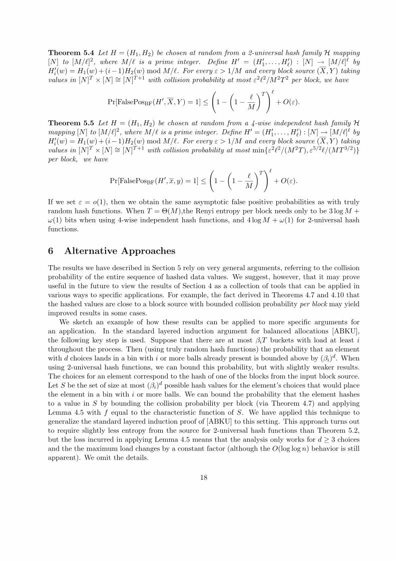
Theorem 5.4 Let H = (H1,H2) be chosen at random from a 2-universal hash family H mapping[N ] to [M/`]2, where M/` is a prime integer. Define H ′ = (H ′

1, . . . ,H′`) : [N ] → [M/`]` by

H ′i(w) = H1(w)+(i−1)H2(w) mod M/`. For every ε > 1/M and every block source (X, Y ) taking

values in [N ]T × [N ] ∼= [N ]T+1 with collision probability at most ε2`2/M2T 2 per block, we have

Pr[FalsePosBF(H ′, X, Y ) = 1] ≤(

1−(

1− `

M

)T)`

+ O(ε).

Theorem 5.5 Let H = (H1,H2) be chosen at random from a 4-wise independent hash family Hmapping [N ] to [M/`]2, where M/` is a prime integer. Define H ′ = (H ′

1, . . . , H′`) : [N ] → [M/`]` by

H ′i(w) = H1(w)+(i−1)H2(w) mod M/`. For every ε > 1/M and every block source (X, Y ) taking

values in [N ]T × [N ] ∼= [N ]T+1 with collision probability at most minε2`2/(M2T ), ε5/2`/(MT 3/2)per block, we have

Pr[FalsePosBF(H ′, x, y) = 1] ≤(

1−(

1− `

M

)T)`

+ O(ε).

If we set ε = o(1), then we obtain the same asymptotic false positive probabilities as with trulyrandom hash functions. When T = Θ(M),the Renyi entropy per block needs only to be 3 log M +ω(1) bits when using 4-wise independent hash functions, and 4 log M + ω(1) for 2-universal hashfunctions.

6 Alternative Approaches

The results we have described in Section 5 rely on very general arguments, referring to the collisionprobability of the entire sequence of hashed data values. We suggest, however, that it may proveuseful in the future to view the results of Section 4 as a collection of tools that can be applied invarious ways to specific applications. For example, the fact derived in Theorems 4.7 and 4.10 thatthe hashed values are close to a block source with bounded collision probability per block may yieldimproved results in some cases.

We sketch an example of how these results can be applied to more specific arguments foran application. In the standard layered induction argument for balanced allocations [ABKU],the following key step is used. Suppose that there are at most βiT buckets with load at least ithroughout the process. Then (using truly random hash functions) the probability that an elementwith d choices lands in a bin with i or more balls already present is bounded above by (βi)d. Whenusing 2-universal hash functions, we can bound this probability, but with slightly weaker results.The choices for an element correspond to the hash of one of the blocks from the input block source.Let S be the set of size at most (βi)d possible hash values for the element’s choices that would placethe element in a bin with i or more balls. We can bound the probability that the element hashesto a value in S by bounding the collision probability per block (via Theorem 4.7) and applyingLemma 4.5 with f equal to the characteristic function of S. We have applied this technique togeneralize the standard layered induction proof of [ABKU] to this setting. This approach turns outto require slightly less entropy from the source for 2-universal hash functions than Theorem 5.2,but the loss incurred in applying Lemma 4.5 means that the analysis only works for d ≥ 3 choicesand the the maximum load changes by a constant factor (although the O(log log n) behavior is stillapparent). We omit the details.

18

7 Conclusion

We have started to build a link between previous work on randomness extraction and the practicalperformance of simple hash functions, specifically 2-universal hash functions. While we expectthat our results can be further improved, they already give bounds that appear to apply to manyrealistic hashing scenarios. In the future, we hope that there will be a collaboration between theoryand systems researchers aimed at fully understanding the behavior of hashing in practice. Indeed,while our view of data as coming from a block source is a natural initial suggestion, theory–systemsinteraction could lead to more refined and realistic models for real-life data (and in particular,provide estimates for the amount of entropy in the data). A complementary direction is to showthat hash functions used in practice (such as those based on cryptographic functions, which maynot even be 2-universal) behave similarly to truly random hash functions for these data models.Some results in this direction can be found in [DGH+].

Acknowledgments

We thank Adam Kirsch for his careful reading of and helpful comments on the paper.

References

[ABKU] Y. Azar, A. Z. Broder, A. R. Karlin, and E. Upfal. Balanced Allocations. SIAM Journalon Computing, 29(1):180–200, 2000.

[BBR] C. H. Bennett, G. Brassard, and J.-M. Robert. Privacy amplification by public discussion.SIAM Journal on Computing, 17(2):210–229, 1988. Special issue on cryptography.

[Blo] B. H. Bloom. Space/Time Trade-offs in Hash Coding with Allowable Errors. Communi-cations of the ACM, 13(7):422–426, 1970.

[BS] A. Blum and J. Spencer. Coloring random and semi-random k-colorable graphs. Journalof Algorithms, 19(2):204–234, 1995.

[BM1] A. Broder and M. Mitzenmacher. Using multiple hash functions to improve IP lookups.In INFOCOM 2001: Proceedings of the Twentieth Annual Joint Conference of the IEEEComputer and Communications Societies, pages 1454–1463, 2001.

[BM2] A. Broder and M. Mitzenmacher. Network Applications of Bloom Filters: A Survey.Internet Mathematics, 1(4):485–509, 2005.

[CW] J. L. Carter and M. N. Wegman. Universal classes of hash functions. Journal of Computerand System Sciences, 18(2):143–154, 1979.

[CG] B. Chor and O. Goldreich. Unbiased Bits from Sources of Weak Randomness and Proba-bilistic Communication Complexity. SIAM J. Comput., 17(2):230–261, Apr. 1988.

[DKSL] S. Dharmapurikar, P. Krishnamurthy, T. Sproull, and J. Lockwood. Deep packet inspec-tion using parallel bloom filters. IEEE Micro, 24(1):52–61, 2004.

19

[DW] M. Dietzfelbinger and P. Woelfel. Almost random graphs with simple hash functions. InSTOC ’03: Proceedings of the thirty-fifth annual ACM symposium on Theory of computing,pages 629–638, New York, NY, USA, 2003. ACM Press.

[DGH+] Y. Dodis, R. Gennaro, J. Hastad, H. Krawczyk, and T. Rabin. Randomness Extractionand Key Derivation Using the CBC, Cascade and HMAC Modes. In M. K. Franklin,editor, CRYPTO, volume 3152 of Lecture Notes in Computer Science, pages 494–510.Springer, 2004.

[GB] G. Gonnet and R. Baeza-Yates. Handbook of algorithms and data structures: in Pascaland C. Addison-Wesley Longman Publishing Co., Inc. Boston, MA, USA, 1991.

[ILL] R. Impagliazzo, L. A. Levin, and M. Luby. Pseudo-random Generation from one-way func-tions (Extended Abstracts). In Proceedings of the Twenty First Annual ACM Symposiumon Theory of Computing, pages 12–24, Seattle, Washington, 15–17 May 1989.

[IZ] R. Impagliazzo and D. Zuckerman. How to Recycle Random Bits. In 30th Annual Sympo-sium on Foundations of Computer Science, pages 248–253, Research Triangle Park, NorthCarolina, 30 Oct.–1 Nov. 1989. IEEE.

[KM] A. Kirsch and M. Mitzenmacher. Less Hashing, Same Performance: Building a BetterBloom Filter. In Proceedings of the 14th Annual European Symposium on Algorithms,pages 456–467, 2006.

[Knu] D. Knuth. The Art of Computer Programming, Volume 3: Sorting and Searching. AddisonWesley Longman Publishing Co., Inc. Redwood City, CA, USA, 1998.

[Mut] S. Muthukrishnan. Data Streams: Algorithms and Applications. Foundations and Trendsin Theoretical Computer Science, 1(2), 2005.

[NT] N. Nisan and A. Ta-Shma. Extracting Randomness: A Survey and New Constructions.Journal of Computer and System Sciences, 58(1):148–173, 1999.

[NZ] N. Nisan and D. Zuckerman. Randomness is Linear in Space. J. Comput. Syst. Sci.,52(1):43–52, Feb. 1996.

[OP] A. Ostlin and R. Pagh. Uniform hashing in constant time and linear space. Proceedingsof the thirty-fifth annual ACM symposium on Theory of computing, pages 622–628, 2003.

[PPR] A. Pagh, R. Pagh, and M. Ruzic. Linear probing with constant independence. In STOC’07: Proceedings of the thirty-ninth annual ACM symposium on Theory of computing,pages 318–327, New York, NY, USA, 2007. ACM Press.

[PR] R. Pagh and F. Rodler. Cuckoo hashing. Journal of Algorithms, 51(2):122–144, 2004.

[Ram1] M. V. Ramakrishna. Hashing practice: analysis of hashing and universal hashing. InSIGMOD ’88: Proceedings of the 1988 ACM SIGMOD international conference on Man-agement of data, pages 191–199, New York, NY, USA, 1988. ACM Press.

[Ram2] M. V. Ramakrishna. Practical performance of Bloom filters and parallel free-text search-ing. Communications of the ACM, 32(10):1237–1239, 1989.

20

[RFB] M. V. Ramakrishna, E. Fu, and E. Bahcekapili. Efficient Hardware Hashing Functions forHigh Performance Computers. IEEE Trans. Comput., 46(12):1378–1381, 1997.

[SV] M. Santha and U. V. Vazirani. Generating Quasi-random Sequences from Semi-randomSources. J. Comput. Syst. Sci., 33(1):75–87, Aug. 1986.

[SS] J. P. Schmidt and A. Siegel. The Analysis of Closed Hashing under Limited Randomness(Extended Abstract). In STOC, pages 224–234. ACM, 1990.

[Sha] R. Shaltiel. Recent Developments in Explicit Constructions of Extractors. Bulletin of theEuropean Association for Theoretical Computer Science, 77:67–95, June 2002.

[Sie] A. Siegel. On universal classes of extremely random constant-time hash functions. SIAMJournal on Computing, 33(3):505–543 (electronic), 2004.

[ST] D. A. Spielman and S.-H. Teng. Smoothed analysis of algorithms: why the simplexalgorithm usually takes polynomial time. Journal of the ACM, 51(3):385–463 (electronic),2004.

[TZ] M. Thorup and Y. Zhang. Tabulation based 4-universal hashing with applications to sec-ond moment estimation. In Proceedings of the Fifteenth Annual ACM-SIAM Symposiumon Discrete Algorithms, pages 615–624 (electronic), New York, 2004. ACM.

[Voc] B. Vocking. How asymmetry helps load balancing. Journal of the ACM, 50(4):568–589,2003.

[WC] M. N. Wegman and J. L. Carter. New hash functions and their use in authenticationand set equality. Journal of Computer and System Sciences, 22(3):265–279, 1981. Specialissue dedicated to Michael Machtey.

[Woe] P. Woelfel. Asymmetric balanced allocation with simple hash functions. In SODA ’06:Proceedings of the seventeenth annual ACM-SIAM symposium on Discrete algorithms,pages 424–433, New York, NY, USA, 2006. ACM Press.

[Zuc] D. Zuckerman. Simulating BPP Using a General Weak Random Source. Algorithmica,16(4/5):367–391, Oct./Nov. 1996.

21