1979

Ecology, 97(8), 2016, pp. 1979–1993© 2016 by the Ecological Society of America

Why species tell more about traits than traits about species: predictive analysis

James s. Clark1,2,3

1Nicholas School of the Environment, Duke University, Durham, North Carolina 27709 USA2Department of Statistical Science, Duke University, Durham, North Carolina 27709 USA

Abstract. Trait analysis aims to understand relationships between traits, species di-versity, and the environment. Current methods could benefit from a model- based proba-bilistic framework that accommodates covariance between traits and quantifies contributions from inherent trait syndromes, species interactions, and responses to the environment. I develop a model- based approach that separates these effects on trait diversity. Application to USDA Forest Inventory and Analysis (FIA) data in the eastern United States demon-strates an apparent paradox, that the analysis of species better explains and predicts traits than does direct analysis of the traits themselves; trait data contain less, not more, infor-mation than species on environmental responses. Whereas variation in some traits is dom-inated by inherent syndromes (tendency for certain traits to be associated with others within an individual and species), others are strongly controlled by variation in species diversity. There is substantial variation in environmental control on trait patterns, between traits and regionally. In terms of environmental response traits do not aggregate into defined plant functional types, as would be desirable for models.

Key words: climate effects; forests; generalized joint attribute modeling; joint species distribution; predic-tive trait analysis; species diversity; trait hyper-volume.

IntroduCtIon

Can analysis of ecological traits explain the diversity of communities in ways that study of species cannot? If distributions of traits provide more direct information on function than do distributions of the species that possess them, they may clarify some mechanisms (Kraft et al. 2008, Mokany et al. 2008, Lamanna et al. 2014) and simplify biodiversity in models to a few trait- defined plant functional types (PFTs) (Boulangeat et al. 2012). Alternatively, a small number of traits that are weakly linked to fitness may provide limited insight on com-munity diversity (Bret- Harte et al. 2008, Kraft et al. 2015). While studies increasingly strive to explain how species and traits are controlled by the environment (Swenson et al. 2012, Lamanna et al. 2014), we do not yet have model- based estimates even for basic quantities, such as how trait covariances depend on the environment. Studies find weak effects of environmental variables at best and lack estimates of uncertainty. Lack of uncer-tainty estimates makes it hard to say how much variation is meaningful. Here I demonstrate that probabilistic models can provide an objective basis for evaluating the connections between species, traits, and the environment. Application to forest inventory data demonstrates how their influences vary geographically and strong and coherent effects of environment and species diversity.

Model- based analysis is developed here to quantify the variation in traits that comes from (1) trait syndromes, (2) the diversity of species that possess them, and (3) the environmental variation that affects both species and trait diversity. Ecological traits are attributes of organisms that vary within individuals, between individuals, and between species (Wright et al. 2004, 2007, Westoby and Wright 2006, Lavorel et al. 2008, Albert et al. 2010, Asplund and Wardle 2014, Mitchell and Bakker 2014, Stahl et al. 2014, Moran et al. 2016), but they are most often analyzed as attributes of locations (Fig. 1a). In other words, there is a trait value associated with a location on a map, but it is derived from values asso-ciated with individuals of a species. Trait syndromes describe how trait variation is structured within and between species (Westoby et al. 2002). They are summa-rized by means, variances, or distributions over indi-viduals of a species, without reference to location. For example, species differences in nutrient requirements lead to covariance between individuals in foliar nitrogen and phosphorus (Reich et al. 1998, Reich and Oleksyn 2004, Han et al. 2005). Species having low wood density may tend to grow rapidly or possess other structural attributes (Chave et al. 2009, Poorter et al. 2010). Some trait covariance could have a phylogenetic component (Rafferty and Ives 2013). The term species diversity is used here in the usual sense of both numbers of species (richness) and evenness (Pielou 1977). Increasing richness can increase trait diversity, as new species bring new trait values. However, for a given number of species, trait diversity decreases with decreasing evenness, as the

Manuscript received 13 January 2016; revised 18 March 2016; accepted 21 March 2016. Corresponding Editor: N. J. B. Kraft.

3 E-mail: jimclark@duke.edu

1980 Ecology, Vol. 97, No. 8 JAMES S. CLARK

distribution of trait values is concentrated around those of the dominant species. Finally, some of that covariance is explained by environmental variation, through its effects on the species that possess both the traits that are measured in a study and also those that are not. Thus, trait syndromes reference individuals whereas the effects of species diversity and environmental on trait distribu-tions reference locations.

The model- based approach provided here quantifies the joint distribution of species and traits data that are measured on different scales. The joint distribution is needed not only to identify effects of trait syndromes, species diversity, and environment, but also to accom-modate the codependence between traits that is induced by the methods used to derive location- referenced trait values as community-weighted means (CWMs). An analysis of climate effects on traits entails a scale trans-lation from measurements on individuals to locations. This transfer is often done using CWMs, the weights being species abundances for a location (Garnier et al. 2004, Ackerly and Cornwell 2007, Díaz et al. 2007, Kraft et al. 2008, Lavorel et al. 2008, Swenson and Weiser 2010, Rainford and Blossey 2014, van Bodegom et al. 2014, Wilfahrt et al. 2014). In RLQ analysis, a sample- by- traits CWM matrix is obtained as the product of a sample- by- species matrix (L) and a species- by- trait matrix (Q′; Doledec et al. 1996, Legendre et al. 1997, Laliberté and Legendre 2010, Lebrija- Trejos et al. 2010, Roscher et al. 2012, Dray et al. 2014). The translation from envi-ronment to traits involves a third matrix, R, the sample- by- environment matrix. Sometimes trait values are assigned to locations based on whether or not a species might occur there (Lamanna et al. 2014); in this case, weights are zeros and ones. Such location- referenced trait values are analyzed in a variety of ways; for simplicity, I refer to CWM analysis, recognizing that CWMs are not the basis for all trait studies, but nonetheless are the subject of a large literature. In each of these cases trans-lating traits from individual measurements to locations induces covariance between CWM values, because values for multiple traits are obtained from the same species data, the same weights.

Joint analysis is complicated by the fact that trait and species data come in many forms. Just as species abun-dance data may be continuous (basal area, density, biomass), discrete (number of individuals), composition (relative abundance), or presence–absence (Clark 2016), trait data can likewise involve different data types. Continuous traits can include specific leaf area (SLA), wood density, leaf chemistry, and maximum tree height. Leaf habit is a categorical trait. Examples include broadleaf deciduous, broadleaf evergreen, and needleleaf evergreen (Fig. 1). When categorical traits are converted into CWM values, they become composition data—the continuous categories sum to 1 (Aitchison 1986, Leininger et al. 2013). Other variables are ordinal, lacking an absolute scale, such as shade tolerance (Baker 1949, Russell et al. 2014). Ordinal variables cannot be analyzed

as quantitative data unless the scale itself is modeled as part of the analysis (Lawrence et al. 2008, Schick et al. 2013).

In the absence of probability- based models to syn-thesize the joint distribution of many data types inter-pretations have relied on randomized versions of data and descriptive methods. Creative approaches include correlation, cluster analysis, ordination, machine- learning algorithms, and other exploratory techniques (Garnier et al. 2004, Wright et al. 2007, Chave et al. 2009, Albert et al. 2010, Kleyer et al. 2012, Swenson et al. 2012, Stahl et al. 2013, Russell et al. 2014). RLQ analysis has the appeal of incorporating multiple traits. However, these methods do not yield probability statements. There are some model- based analyses of CWM values, but they lack a joint distribution. Generalized linear models fitted for each trait independently or for traits as predictors of species presence/absence (Webb et al. 2010, Pollock et al. 2012, Jamil et al. 2013, Zhu et al. 2014) miss probabilistic relationships between traits. Current models do not accommodate the fact that CWM variation between samples (Fig. 1a) can be subtle relative to the large dis-persion within samples (Fig. 1b). A joint distribution is needed that accommodates not only variation in traits, but covariance between traits, within a model framework.

This paper provides model- based trait inference and probabilistic prediction, which quantifies dependence in trait syndromes, species diversity, and environment and provides a basis for evaluating hypotheses (Ackerly and Cornwell 2007, Kraft et al. 2008, 2015, Lamanna et al. 2014). Inference refers to fitting a model to estimate parameters with uncertainty. Predictive distributions are used to evaluate the model in- and out- of- sample and to evaluate its implications outside where data are observed. The uncertainty that can be estimated for parameters and predictions is important for hypothesis testing, e.g., by comparing fits for models that describe different relation-ships. I begin by summarizing unique aspects of trait analysis that benefit from a joint analysis. Current CWM analyses often involve comparisons with environmental gradients or species diversity. I show why more insight is available from analyses of species, followed by trait prediction. The example application to eastern U.S. forests quantifies the contributions of environment to trait and species diversity. It demonstrates that the dis-tributions of species are more sensitive to the environment than are the distributions of traits and shows how trait data can be effectively interpreted.

traIt data and models

The paradoxical conclusion that CWM analysis can be most informative when it begins with species rather than traits results from how stochasticity is treated in a trait model. A CWM analysis obtains trait values for a location by weighting species traits by the relative abun-dance of each species. Consider a single trait value tms, for trait m = 1,…, M measured on each of s = 1,…, S

August 2016 1981PREDICTIVE TRAIT ANALYSIS

FIg. 1. (a) Trait norms (TN; Eq. S2) and (b) ratio of the square- root of trait codispersion (WTC; Eq. S5) divided by TN, a coefficient of variation. In (b), contours are from thin to fat, 0.1, 1, 10. SLA, specific leaf area.

Seed mass

−1.8

1.3Dry wood density

−1.8

1.2

Maximumheight

−0.8

2.3

Leaf [N]

−1.9

1.3Leaf [P]

−1.2

1.5

SLA

−1.6

1.6

3035

4045

Seed mass

0

5

Dry wooddensity

0

5

Maximumheight

0

5

−95 −90 −85 −80 −75 −70

3035

4045

Leaf [N]

0

5

−95 −90 −85 −80 −75 −70

Leaf [P]

0

5

−95 −90 −85 −80 −75 −70

SLA

0

5

1982 Ecology, Vol. 97, No. 8 JAMES S. CLARK

species. Together these trait values are organized as an M × S matrix T of trait syndromes by species. Each trait occupies one row of T, a length-S vector tm. Weights are contained in the length-S vector wi at locations i = 1,…, n. Weights can be relative abundances of each species. The CWM value for trait m at location i is

(1)

The weight represented by the abundance of each species affects the CWM values for all traits and thus induces co- dispersion. The trait values obtained in this manner can be modeled jointly. However, the stochas-ticity in traits does not come from the trait data, suggesting an alternative approach.

What’s random, and why it matters

The stochasticity in CWM analysis does not come from traits. This is important because probabilistic models treat observations as random and independent. A standard weighted mean is obtained by weighting random observations unevenly, with the sum- to- one con-straint on weights. The weights are taken to be fixed, and the sample is random. In CWM analysis, the opposite is true—species abundances are random, and the trait values in matrix T are taken as fixed—the same matrix T is applied to all sample locations. The CWM not only translates traits from individuals of a species to locations. It also changes the covariance structure of data. I first discuss why the change in reference affects the trait analysis, followed by the effect of CWM on model covariance.

To estimate the effect of environment ei on species si and trait mi requires that all three variables be referenced by location i. To predict species and traits from envi-ronment, we need the conditional distribution

For example, to understand the effect of temperature or moisture (e) on a foliar chemistry trait (m), we could obtain a random sample of leaves recovered from litter traps, referenced by the location of the trap. The trait value could be recorded for each leaf. A model of

[si,mi|ei

]

could relate the trait values directly to the environment at each location.

A reference problem arises because trait values are rarely obtained this way. Individuals are sampled, not leaves, are selected for sampling. Let (i) be the index for an individual selected for sampling at location (i). Individuals on the basis of all three variables, a condi-tional distribution

and leaves are measured on the sampled individual. Species and traits affect which individuals are sampled when studies focus on particular species groups, life

forms, and so on. Environment affects sampling because it affects which species and trait values are common, and the environments included in a study are typically taken as part of the study design. The species- trait model is now problematic because traits and species depend on which individuals are in the data, related by conditional distributions,

In the special case where individuals are selected at random and all individuals contribute to trait values in the same way, then the distribution is simplified to some-thing more like the litter trap example. Consider ran-domly located plots, each containing ni individuals. Then if individuals are selected at random, and each individual has a probabiliity 1/ni of being selected, and the proba-bility does not depend on other variables.

In this case we have the proper conditional distri-bution, which, like the leaf example, does not depend on individuals

(2)

Usually we do not have this distribution, due to two problems: (A) individuals are not selected at random and (B) each individual contributes to the mean trait value at a location differently. Problem A means we cannot ignore the design. Problem B means that individual meas-urements require some form of weighting.

Trait reference and non- ignorable design

Ignorable design is an important concept for trait analysis, because trait values depend on climate and species (that’s usually the point), and these variables have biased representation in literature compilations. In the foregoing example of foliar chemistry, a model for trait response to soil fertility could come from litter traps deployed along a gradient. The model can ignore sampling design if the response is effectively the same as would have been obtained if sampling had been done at different locations along the gradient. Likewise, sampling leaves at random from litter traps allows us to ignore individuals and species, due to the manner in which samples are obtained. A model of envi-ronment effects on traits could take the measured trait values on leaves and scale them by the total weight of the sample to obtain location- referenced trait values. Again, the sample need not be referenced to an indi-vidual or even a species. However, design cannot be ignored if samples are concentrated in part of the gra-dient, on specific species, or specific individuals, because sample distribution determines parameter

umi=

S∑

s=1

tms

wis= t

m

wi

[si,mi|ei

].

[Ii|si,mi,ei

]

si,mieiIi

=

Iisi,mi,ei

si,mi,ei

∑s,t

Iisi,mi,ei

si,mi,ei

[Ii|si,mi,ei

]=[Ii

]=n−1

i.

si,miei

=

n−1i

si,mi,ei

n−1i

∑s,t

si,mi,ei

=si,mi,ei

ei

.

August 2016 1983PREDICTIVE TRAIT ANALYSIS

estimates. Problems compound if the studies used to compile trait data target specific species, which is almost always the case.

Individuals are not identical

Even where individuals are sampled at random, a model of environment effects on traits requires a means for scaling the sampled leaves to obtain their contri-bution to total leaves at the location. This scaling requires that individuals can be weighted in terms of the number (or mass) of leaves they hold. Ideally, the weights approximate the contribution of each individual to the location- referenced trait. Whereas wood density might be scaled by its biomass of the individual, seed mass might be scaled by fecundity, including zeros for non- reproductive individuals. The species- specific weights (e.g., allometric coefficients) introduce covariance between traits that does not exist in the true values. The CWM values have induced covariance that results from use of the same species weights for multiple traits.

Eq. 1 is a deterministic transformation of random species abundance by a fixed trait matrix T. Rather than a weighted mean, the CWM is more accurately described as a variable change, a standard term for variables (traits) that inherit the distribution of other variables (species abundances) as a simple functional relationship. CWM trait values do not have means and variances in the usual sense (they result from a variable change), but they can be described by norms and dispersion (Appendix S1). In this paper, trait syndromes are described by the trait norm (TN) and trait co-dispersion (TC; Table 1). I use the terms “mean” and “variance” when discussing variables that could be random in a model. CWM analysis weights the trait norm by species abundance

in a sample, termed the weighted trait norm (WTN) and weighted trait co-dispersion (WTC). The concepts of TN and TC are valuable as baselines for considering species and environment effects.

Recognizing that stochasticity in CWM traits ema-nates from weights suggests both limitations and oppor-tunities. Limitations include the fact that, independent of species, traits obtained as CWM values do not have distributions. Trait values for a location reflect species turnover in space and, unless design can be ignored, species selection by ecologists. Maps like Fig. 1 are maps of species, not traits. So “trait modeling” can be viewed as “weight modeling”; the variation in traits is induced by weights. The realization that trait models are ulti-mately weight models suggests the opportunity. If non- ignorable design and weighting can be addressed, then the translation from individuals to locations in Eq. 1 can happen before or after analysis. Our analysis addresses the design challenges with use of a uniform sample grid over the sub- continent. Use of CWM values, based on biomass of each individual, shifts reference from plants to locations. Variation within species is not included in this analysis, due to availability of data. However, con-structing a model for traits and species given environment with intraspecific variation has to confront these same issues (see Discussion). By fully evaluating both approaches, I show the paradox: we can learn more about traits from the indirect model of species than from the direct model of CWM traits themselves. I use the term trait response model (TRM) for the model where translation comes first. I use the term predictive trait model (PTM) for the model where translation comes last. Before describing each, I summarize the design consid-erations for trait analysis.

table 1. Variables and sources of dispersion and variance in trait formulas, including model- based inference.

Source Eq. Size Description Uncertainty

Samples and transformations

Trait observation (ti) 1 M × 1 trait vector at location i data (if replicate measurements)

Relative species abundance (wi) 1 S × 1 species vector at location i data (if replicate plots) Trait matrix (T) 7, 8, S2 M × S traits by species matrix fixed Predictors (xi) 3, 6 Q × 1 design vector at location i fixed

Inherent trait syndromes

Trait norm (TN) S2 M × 1 average over species no Trait co- dispersion (TC) S4 M × M average squared distance from TN noSample weighted traits Weighted trait norm (WTN) or

community weighted meanS3 M × 1 weighted by a species sample no

Weighted trait co- dispersion (WTC) S5 M × M average squared distance from WTN no

Model- based estimates

Predictive covariance (PTC) S8 M × M covariance from inherent syndromes, species diversity, and environment

data, model, parameters

Environmental trait covariance (ETC) and species covariance (ESC)

S9 M × M covariance explained by environmental predictors

data, model, parameters

Note: Dimensions are given for Q predictors, M traits, and S species.

1984 Ecology, Vol. 97, No. 8 JAMES S. CLARK

Model- based inference and prediction

Both the trait response model (TRM) and the pre-dictive trait model (PTM) described here begin with species composition data and lead to model- based esti-mates (TRM) or predictions (PTM) of covariances for the joint distribution of traits. The length-S vector wi in Eq. 1 contains relative species abundances in observation i. The TRM translates S species to a length-M vector of traits, ui = Twi first and then models traits as a combi-nation of discrete and continuous data types. The PTM models species weights as composition data and then predicts traits. The generalized joint attribution model (gjam) was used for both TRM and PTM. gjam accom-modates combinations of continuous, categorical, com-position, and ordinal data on the observation scales (Clark 2016; Appendix S1).

In TRM, traits are response variables. Seed mass, wood density, maximum height, foliar chemistry, and specific leaf area (SLA) are continuous variables. In this analysis, they are centered and standardized. Dioecy and ring- porous xylem anatomy are categorical variables, both with two classes. Leaf habit has three classes (broadleaf deciduous, needleleaf evergreen, broadleaf evergreen). Categorical traits become composition data when transformed by weights, fractions that sum to one. Ordinal traits include shade, drought, and flood tol-erance scores, based on five classes (Niinemets and Valladares 2006, Stahl et al. 2013, Russell et al. 2014). Although modeled as continuous variables in previous trait analyses, ordinal traits cannot be averaged or modeled with regression, because they have no scale—the difference between a score of 1 and 2 (e.g., “very intol-erant” and “intolerant”) does not equal the difference between 2 and 3 (e.g., “intolerant” and “intermediate”). We use the original five categories for shade- , flood- , and drought- tolerance (Baker 1949, Russell et al. 2014) and model them in gjam as ordinal data (Appendix S1). Because CWMs cannot be used for ordinal data each plot is assigned the modal tolerance score obtained using the CWM values as weights on each tolerance class. These are “community- weighted modes.”

Joint modeling of combined data types is detailed in Clark et al. (2016, in review). The first stage model is a multivariate normal distribution. The vector of traits at location i is

(3)

where α is a Q × M matrix of coefficients, xi is the length Q vector of predictors, and Ω is an M × M trait covariance matrix. Continuous values in vector ui are the trait values themselves (continuous traits) or they determine the values for discrete traits vim defined by a partition pm,k for the kth level of trait m

(4)

(5)

Whereas TRM translates weights to traits first and then models traits, PTM models weights first, translates to traits second, and predicts traits third. Eq. 3 becomes

where β is a Q × S matrix of coefficients, and Σ is an S × S species covariance matrix. Continuous values in vector wi are the relative species weights. Once the species model is fitted, the translation to traits is a variable change

(7)

(8)

Thus, the model is fitted to species weights then trans-formed to traits.

The third step involves trait prediction, which quantifies the contribution of species diversity to trait diversity (Appendix S1). Trait prediction provides a model- based version of WTC in Eq. 5. From this we derive the predictive trait covariance (PTC) and the environmental trait covar-iance (ETC), which can be expressed as a fraction of the total model- based variance, the relative ETC, or RETC. Likewise the relative environmental species covariance is RESC.

Species and environment contributions to trait diversity

The framework laid out here includes the inherent trait syndromes (TC), the effects contributed by species dis-tribution and abundance (PTC), and the effects of envi-ronment that operates through its impact on species distribution (ETC; Table 1). Importantly, all of these contributions are on the same scale as the trait data; we can interpret effects of environment x and trait corre-lation Ω on the same scale as the traits themselves.

The most important distinction between traditional CWM analysis and both of the methods used here is the model. Weighted trait codispersion (WTC; Eq. S5) describes codispersion in traits induced by empirical species abundances (W). By contrast, the model- based PTC (Eq. S8) describes trait diversity in terms of species responses to environment with full posterior inference available for β and Σ, which can be decomposed into species and envi-ronment effects. The effect of environmental variable q on trait m is

i.e., the sum of the effects of each species. The effect of species s is isolated as pmsq = tmsβsq. The ability to isolate how each species contributes can be an advantage of PTM.

Evaluating the effect of a predictor taken over all species and traits requires too many coefficients and no way to combine them. Inverse prediction (Clark et al. 2012, 2013) provides sensitivity of all traits to a predictor in x. The number of sensitivity coefficients for a multivariate response can be large, e.g., S × Q coefficients for species or M × Q coefficients for traits. They cannot be added together or

ui∼MVN

(

xi,Ω

)

vim =k pm,k ≤uim <pm,k+1 (discrete class)

tim=

u

imcontinuous trait

vim

discrete trait(observations)

(6)wi∼MVN

(xi,Σ

)

=T

=TΣT.

um

xq

=Tmq

August 2016 1985PREDICTIVE TRAIT ANALYSIS

averaged. By inverting the model, inverse prediction reduces sensitivity analysis to Q coefficients, each describing how the full ensemble of traits and species responds to a predictor. I use Brynjarsdottir and Gelfand’s (2015) index, the variance term in Clark et al.’s (2013) sensitivity index, for the TRM

and the PTM

I predict sensitivity s in eqns 9a, b from both models. In the application that follows, I demonstrate their rela-tionships to one another.

The model- based analysis quantifies how species diversity and environment affect the covariance in traits. Trait syndromes for the species present at a local site or within a region occupy a cloud in trait space (Hutchinson 1957, Mouillot et al. 2005, Lamanna et al. 2014). That cloud has hyper- volume V(TC), where TC is the trait covariance for species that occur in the region. (Appendix S1). The volume of that cloud is increased by species richness and by species evenness. Conversely, species dominance reduces trait diversity. This reduction in trait volume can result from “filtering” of species possessing certain trait values (Dias et al. 1998, Cornwell and Ackerly 2009). The hyper- volume of traits that includes effects of species diversity is V(WTC) (empirical weights) or V(PTC) (model- based estimate). Finally, the volume that is explained by the environmental inputs is V(ETC).

Simple indices summarize the effects on trait diversity on the trait cloud V(). Inherent trait diversity occupies a hyper- volume on a per- species basis,

The maximum hyper- volume obtains at maximum entropy, all species equally abundant. This covariance is TC. Species diversity reduces the inherent diversity from potential TC to actual WTC. The reduction is greatest when this index is large

The effect of the environment is large when it repre-sents a large fraction of the inherent trait diversity:

methods

I illustrate using data from the USDA Forest Inventory and Analysis (FIA) program, climate from PRISM (data available online),4 and trait data, described in the

Appendix S1. The trait response model (TRM, Eq. 3) and the predictive trait model (PTM, Eq. 6) were both fitted to the data using generalized joint attribute mod-eling (gjam in R, Appendix S1). For this illustration, I include main effects from variables in Table S1, including interactions between moisture and soil type, a multilevel factor (four levels). Five percent of data were reserved for out- of- sample prediction. Diagnostics are presented with results in the next section.

results

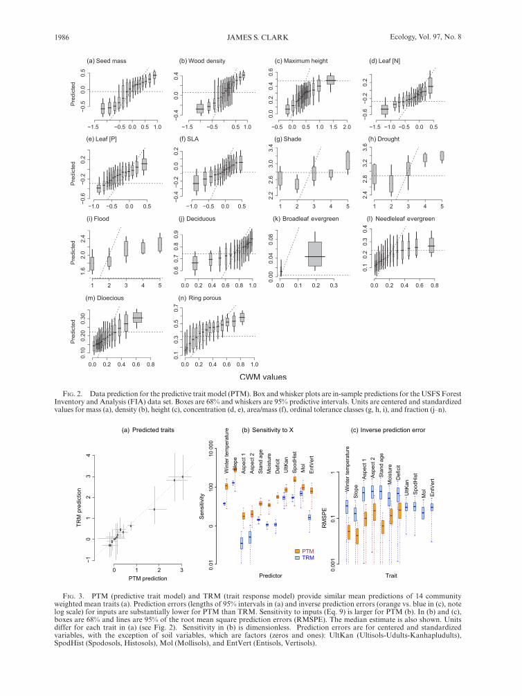
The two methods differ in their sensitivity to environ-mental variables and predictive capacity. Both models predict most traits well, those for the predictive trait model (PTM) shown in Fig. 2. Predictions are least accurate at extremes, where there are few data. Poorest predictions are for ordinal tolerance classes (Fig. 2g–i). The model includes local and regional site factors that might be expected to predict these variables, including stand age for shade tolerance, deficit for drought tol-erance, and moisture for flood tolerance. Of the compo-sitional trait leaf types, the rare broadleaf evergreen type is poorly predicted (Fig. 2k).

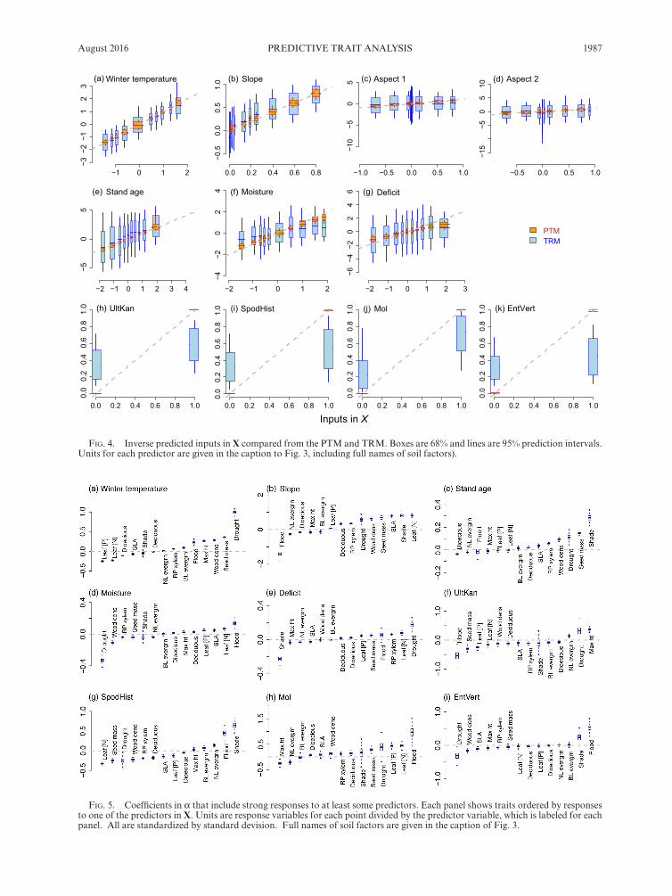
Mean trait predictions are similar for the two models, with prediction errors being smaller for the PTM (Fig. 3a). The PTM finds larger sensitivity to predictors (Fig. 3b) and lower inverse prediction error for inputs in the model X (Fig. 3c). The difference is so wide for soil types that they could not be represented on the same scale with other inputs in Fig. 3c. If a predictor variable accounts for much of the observed response then inverse predictions will be concentrated near the 1:1 line in Fig. 4, as is the case for PTM (orange). Wide predictive intervals indicate low sensitivity for TRM (blue in Fig. 4). The full community of species provides especially accurate predictions of soil type, whereas traits do not (Fig. 4h–k). Despite differences in sensitivity, models agree that, taken across all species, winter temperature, slope, and soils are covariates having the most influence on traits in this analysis (Fig. 3b) and are best predicted by the community of species and traits (Fig. 3c).

Posterior distributions for trait responses to predictors are well identified, with narrow 95% credible intervals (Fig. 5). Although ordinal tolerance classes are not well predicted by the model, they are most sensitive to a number of predictors, probably due in part to definitions: the ordinal classes are partly defined by their tendency to covary with input variables analyzed here (Niinemets and Valladares 2006). Of all traits, drought tolerance shows the strongest positive response to winter temper-ature (Fig. 5a) and climatic deficit (Fig. 5e) and the strongest negative response to moisture (Fig. 5d) and entisol/vertisol soils (Fig. 5i). Flood tolerance shows the strongest positive response to moisture (Fig. 5d), mollisol (Fig. 5h) and entisol/vertisol soils (Fig. 5i) and the strongest negative response to slope (Fig. 5b) and ultisol- udults- kanhapludults soils (Fig. 5f). Shade tolerance

(9a)sTRM =diag(−1

)

(9b)sPTM =diag(T

(TΣT

)−1

T)

(10a)V (TC)

S

(10b)1−V (WTC)

V (TC).

(10c)V (ETC)

V (TC).

4 http://prism.nacse.org/

1986 Ecology, Vol. 97, No. 8 JAMES S. CLARK

FIg. 2. Data prediction for the predictive trait model (PTM). Box and whisker plots are in- sample predictions for the USFS Forest Inventory and Analysis (FIA) data set. Boxes are 68% and whiskers are 95% predictive intervals. Units are centered and standardized values for mass (a), density (b), height (c), concentration (d, e), area/mass (f), ordinal tolerance classes (g, h, i), and fraction (j–n).

(a) (b) (c) (d)

(e) (f) (g) (h)

(i) (j)

(m) (n)

(k) (l)

FIg. 3. PTM (predictive trait model) and TRM (trait response model) provide similar mean predictions of 14 community weighted mean traits (a). Prediction errors (lengths of 95% intervals in (a) and inverse prediction errors (orange vs. blue in (c), note log scale) for inputs are substantially lower for PTM than TRM. Sensitivity to inputs (Eq. 9) is larger for PTM (b). In (b) and (c), boxes are 68% and lines are 95% of the root mean square prediction errors (RMSPE). The median estimate is also shown. Units differ for each trait in (a) (see Fig. 2). Sensitivity in (b) is dimensionless. Prediction errors are for centered and standardized variables, with the exception of soil variables, which are factors (zeros and ones): UltKan (Ultisols-Udults-Kanhapludults), SpodHist (Spodosols, Histosols), Mol (Mollisols), and EntVert (Entisols, Vertisols).

0 1 2 3

−10

12

34

PTM prediction

TRM

pre

dict

ion

(a) Predicted traits

Predictor

Sen

sitiv

ity0.

010

100

10 0

00

PTMTRM

(b) Sensitivity to X

Trait

RM

SP

E0.

001

0.1

1

(c) Inverse prediction error

Win

ter t

empe

ratu

reS

lope

Asp

ect 1

Asp

ect 2

Sta

nd a

geM

oist

ure

Def

icit

UltK

anS

podH

ist

Mol Ent

Ver

t

Slo

peA

spec

t 1A

spec

t 2S

tand

age

Moi

stur

eD

efic

itU

ltKan

Spo

dHis

tM

olE

ntV

ert

Win

ter t

empe

ratu

re

August 2016 1987PREDICTIVE TRAIT ANALYSIS

FIg. 4. Inverse predicted inputs in X compared from the PTM and TRM. Boxes are 68% and lines are 95% prediction intervals. Units for each predictor are given in the caption to Fig. 3, including full names of soil factors).

Inputs in X

−1 0 1 2

−3−2

−10

12

3

0.0 0.2 0.4 0.6 0.8

−0.5

0.0

0.5

1.0

−1.0 −0.5 0.0 0.5 1.0

−10

−50

5

−0.5 0.0 0.5 1.0

−15

−50

510

−2 −1 0 1 2 3 4

−50

5

−2 −1 0 1 2

−4−2

02

4

−2 −1 0 1 2 3

−6−4

−20

24

6

PTMTRM

0.0 0.2 0.4 0.6 0.8 1.0

0.0

0.2

0.4

0.6

0.8

1.0

0.0 0.2 0.4 0.6 0.8 1.0

0.0

0.2

0.4

0.6

0.8

1.0

0.0 0.2 0.4 0.6 0.8 1.0

0.0

0.2

0.4

0.6

0.8

1.0

0.0 0.2 0.4 0.6 0.8 1.0

0.0

0.2

0.4

0.6

0.8

1.0

(a) Winter temperature (b) Slope (c) Aspect 1 (d) Aspect 2

(e) Stand age (f) Moisture (g) Deficit

(h) UltKan (i) SpodHist (j) Mol (k) EntVert

FIg. 5. Coefficients in α that include strong responses to at least some predictors. Each panel shows traits ordered by responses to one of the predictors in X. Units are response variables for each point divided by the predictor variable, which is labeled for each panel. All are standardized by standard devision. Full names of soil factors are given in the caption of Fig. 3.

1988 Ecology, Vol. 97, No. 8 JAMES S. CLARK

shows the strongest positive response to stand age (Fig. 5c) and spodisol- histisol soils (Fig. 5g) and the strongest negative response to climatic deficit (Fig. 5e). In each of these cases at least some of these predictors are used to assign ordinal classes to species, which affects, in turn, the plot CWM value.

The model- based analysis provides estimates and uncertainty for trait variables measured in diverse ways on a common scale, allowing comparisons. The strongest effects on foliar chemistry come from temperature, a negative effect on leaf (N) and leaf [P] (Fig. 5a) and mol-lisol soils, a positive effect (Fig. 5h). However, the overall responses of these foliar traits differ substantially. The environmental trait covariance (ETC) shows that leaf [N] responds like SLA, whereas leaf (P) responds most like

dioecy (Fig. 6). Xylem anatomy, wood density, and seed mass are most similar based on their responses to the environment (Fig. 6). Based on responses to all environ-mental variables there are three distinct clusters of traits shown at the top of Fig. 6.

If traits capture the responses of species to environ-mental predictors, then trait groupings provide a natural classification of plant functional types (PFTs). Fig. 6 shows a clustering based on distance using responses to the same environmental variables, RESC for species (left) and RETC for traits (top), i.e., the responses of species and traits to the environment. The clustering of species based on their responses to the environment is consistent with major forest types in the eastern United States. The clustering of traits is based on the same criteria. If PFTs

FIg. 6. Cluster analysis of species (left) and traits (top) based on the relative environmental trait covariance (RETC,). The table at right shows trait values centered on mean values, with clustering at the top. The main clusters in species and traits are outlined with dashed lines on the grid. Color scale is in units of standard deviations for each trait. Custer distance has units of Dij = ETCii + ETCjj - 2ETCij.

August 2016 1989PREDICTIVE TRAIT ANALYSIS

can summarize responses of species, we expect well- defined blocks of trait–species combinations in Fig. 6. Although there are a few weak patterns (high average wood density and seed mass in southern forests), results do not provide a summary set of PFTs based on traits that could stand in for species groups.

The importance of modeling ordinal variables properly is demonstrated by the partition estimates for the five classes in Fig. 7. There are four values separating five ordinal classes for each variable. The first partition is fixed at a value of 1, separating the first and second classes, but estimates for the other classes are part of the posterior distribution (Clark 2016). The highly nonlinear relationship, with negligible separation for the highest shade- and flood- tolerance classes, comes from two aspects of the data: (1) few plots are assigned to these highest categories, because the modal tolerance class for a plot is rarely the most tolerance class, and (2) the eco-logical separation between high- tolerance classes is weaker than for low- tolerance classes. The ordinal classes cannot be analyzed as an absolute scale, because they are assigned on a qualitative basis. With proper inference, they show strong responses to the environment (Fig. 5).

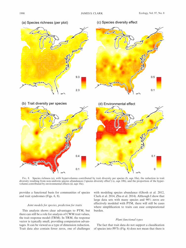
The model- based approach provides a probabilistic basis for evaluating the effects of species diversity and environment on trait diversity. The contributions differ for each trait, but can be summarized across all traits by the volume of the trait cloud (Fig. 8). Taken over all traits, the trait volume per species is highest in the south-eastern and Gulf coastal plain (Fig. 8b). In other words, traits are more tightly packed across the rest of the map. The inherent trait diversity is reduced by species domi-nance least and controlled by environmental variation most in the Midwest (Fig. 8c), with dry climate and fertile soils (mollisols). The effect of the environment is strong where there are species that have large response to the environment (large |β|) and where the variation in climate is large (Q in Eq. S9). The remaining central, northeast, and northern lakes regions have the strongest reductions in trait diversity due to species dominance.

dIsCussIon

The apparent paradox, that a species model better pre-dicts controls on trait responses than do the traits them-selves, is understood from basic principles of aggregation. Ecologists have recently argued to shift attention from species to traits (Mokany et al. 2008, Lebrija- Trejos et al. 2010). Many studies look for pattern in trait data that can explain environmental constraints on species diversity (e.g., Stahl et al. 2013, Lamanna et al. 2014, Kraft et al. 2015). Results presented here help clarify how models can aid analysis of environmental controls on species and trait diversity, including why more is learned about traits from studying species, rather than from analysis of traits directly. It provides perspectives that can guide future analysis and interpretation of trait patterns.

The contrasting performance of TRM and PTM comes from the fact that information is not recovered by analysis of aggregated versions of the same data (Clark et al. 2011). Predictive performance is most critical for evaluating mechanisms, because it most closely addresses the question: “What trait responses result from a given environmental scenario?” Here the contrast between traits vs species analysis is stark (Figs. 3, 4). The many species contributing to the PTM contain information that is unavailable to the TRM. Said another way, many combinations of species are indistinguishable on the basis of CWM values, even when traits are evaluated as a joint distribution. Each species brings information, and, through PTM, that information is available for pre-diction. It includes the fundamental relationships between species and environment that is lost when species are summarized by a few traits. Thus, one can learn more from the species themselves.

It would not be correct to attribute the limitations of CWM analysis solely to methodology. The differences between TRM and PTM result from the fact that a small number of measureable traits cannot explain diversity of large numbers of species. In CWM analysis variability comes solely from the species; traits are everywhere fixed.

The advantage for inverse prediction

The PTM is especially valuable for inverse prediction of inputs in X. No single species or trait could predict local climate, drainage, stand age, slope, aspect, and soil type. Nor could the environment be predicted from inde-pendent models fitted to each tree species or trait. The joint distribution of species can predict all of these vari-ables together and far better than could be done with traits (Fig. 4). The predictive distribution provides a basis for clustering species and traits based on responses to the environment. Environmental trait covariance (ETC)

FIg. 7. The estimated partition for ordinal tolerance classes, each on a five- point scale.

0 2 4 6 8 10Unit variance scale

Dro

ught

Floo

dS

hade

1 2 3 4

1990 Ecology, Vol. 97, No. 8 JAMES S. CLARK

provides a functional basis for communities of species and trait syndromes (Figs. 6, 8).

Joint models for species, prediction for traits

This analysis shows clear advantages to PTM, but there can still be a role for analysis of CWM trait values, the trait response model (TRM). In TRM, the response vector is typically small, providing computation advan-tages. It can be viewed as a type of dimension reduction. Trait data also contain fewer zeros, one of challenges

with modeling species abundance (Ghosh et al. 2012, Clark et al. 2014, Zhu et al. 2014). Although I show that large data sets with many species and 90% zeros are effectively modeled with PTM, there will still be cases where simplification to traits can ease computational burden.

Plant functional types

The fact that trait data do not support a classification of species into PFTs (Fig. 6) does not mean that there is

FIg. 8. Species richness (a), with hypervolumns contributed by trait diversity per species (b, eqn 10a), the reduction in trait diversity resulting from non-uniform species abundances (‘species diversity effect’) (c, eqn 10b), and the proportion of the hyper-volumn contributed by environmental effects (d, eqn 10c).

2.3

9.3

0.1

0.4

0.1

0.5

0

0.1

(a) Species richness (per plot)

(b) Trait diversity per species

(c) Species diversity effect

(d) Environmental effect

August 2016 1991PREDICTIVE TRAIT ANALYSIS

no role for PFTs in models. First, species included in this analysis do not span the range of PFTs that might be used in global models, many clearly differentiated such as C3 and C4 grasses. Still, this analysis does span a broad range of PFTs, and it does not map to responses of species across a broad climate gradient (Fig. 6). The important point here is that a PFT class does not have to respond differently from all others to have potential use in models. Most important in models is that species within a PFT class respond similarly.

Inherent syndromes, species diversity, environmental control

The need to evaluate relationships between traits and species diversity and the environment motivates joint predictive trait modeling. This perspective separates trait syndromes, i.e., codispersion of traits (TC), codis-persion induced by species diversity of a sample (WTC), environmental trait covariance (ETC), and relative envi-ronmental trait covariance (RETC) (Table 1). All can be cast as distance matrices to reveal their relationships to one another (e.g., cluster or correlation analysis; Fig. 6) and geographically (Fig. 8). Inverse prediction provides sensitivity analysis of large trait distributions (Fig. 3b).

Trait variation at the organism scale

Recognition of the importance of trait variation within and between organisms predates the recent increase in trait studies. From variation within organisms (e.g., sun vs. shade leaves, tension vs. compression wood, seed- size variation) and between individuals, as the basis for adaptive evolution, the role of individual variation is critical. Intra- organism and intraspecific variation have been increasingly recognized in trait studies (Mitchell and Bakker 2014, Moran et al. 2016). Because the subject is already large when limiting analysis to CWM trait values, I focus here on variation at the species level. However, biogeographic analysis of intraspecific variation con-fronts the same issues addressed here, including the shift in reference from individuals to locations, proper weighting, and analysis as TRM or PTM.

aCknowledgments

This study was supported by NSF grants EF- 1137364, the Macrosystems Biology program, and the Coweeta LTER. For comments on the manuscript, I thank David Ackerly, Aaron Berdanier, Alan Gelfand, Nathan Kraft, Matt Kwit, Bijan Seyednasrollah, Maria Uriarte, and two anonymous reviewers.

lIterature CIted

Ackerly, D. D., and W. K. Cornwell. 2007. A trait- based approach to community assembly: partitioning of species trait values into within- and among- community components. Ecology Letters 10:135–145.

Aitchison, J. 1986. The statistical analysis of compositional data. Chapman and Hall, New York, New York, USA.

Albert, C. H., N. G. Thuiller, R. Yoccoz, S. Douzet, S. Aubert, and S. Lavorel. 2010. A multi trait approach reveals the struc-ture and the relative importance of intra vs. interspecific vari-ability in plant traits. Functional Ecology 24:1192–1201.

Asplund, J., and J. D. A. Wardle. 2014. Within- species variabil-ity is the main driver of community- level responses of traits of epiphytes across a long- term chronosequence. Functional Ecology 28:1513–1522.

Baker, F. S. 1949. A revised tolerance table. Journal of Forestry 47:179–181.

van Bodegom, P. M., J. C. Douma, and L. M. Verheijen. 2014. A fully traits- based approach to modeling global vegetation distribution. Proceedings of the National Academy of Sciences USA 111:13733–13738.

Boulangeat, I., et al. 2012. Improving plant functional groups for dynamic models of biodiversity: at the crossroads between functional and community ecology. Global Change Biology 18:3464–3475.

Bret-Harte, M. S., M. C. Mack, G. R. Goldsmith, Sloan, D. B., J. DeMarco, G. R. Shaver, P. M. Ray, Z. Biesinger, and F. Stuart Chapin III. 2008. Plant functional types do not predict biomass responses to removal and fertilization in Alaskan tussock tundra. Journal of Ecology 96:713–726.

Brynjarsdottir, J., and A. E. Gelfand. 2015. Collective sensitiv-ity analysis for ecological regression models with multivariate response. 19:479–500. Unpublished manuscript.

Chave, J., D. Coomes, S. Jansen, S. L. Lewis, N. G. Swenson, and A. E. Zanne. 2009. Towards a worldwide wood econom-ics spectrum. Ecology Letters 12:351–366.

Clark, J. S. 2016. Generalized joint attribute modeling (gjam) in R. http://sites.nicholas.duke.edu/clarklab/code/

Clark, J. S., D. M. Bell, M. H. Hersh, M. Kwit, E. Moran, C. Salk, A. Stine, D. Valle, and K. Zhu. 2011. Individual- scale variation, species- scale differences: inference needed to understand diversity. Ecology Letters 14:1273–1287.

Clark, J. S., D. M. Bell, M. Kwit, A. Powell, R. Roper, A. Stine, B. Vierra, and K. Zhu. 2012. Individual- scale inference to anticipate climate- change vulnerability of biodiversity. Philosophical Transactions of the Royal Society B 367:236–246.

Clark, J. S., D. M. Bell, M. Kwit, A. Powell, and K. Zhu. 2013. Dynamic inverse prediction and sensitivity analysis with high- dimensional responses: application to climate- change vulnerability of biodiversity. Journal of Biological, Environmental, and Agricultural Statistics 18:376–404.

Clark, J. S., A. E. Gelfand, C. W. Woodall, and K. Zhu. 2014. More than the sum of the parts: forest climate vulnerability from joint species distribution models. Ecological Applications 24:990–999.

Clark, J. S., D. Nemergut, B. Seyednasrollah, P. Turner, and S. Zhang. 2015. Median- zero, multivariate, multifarious data: generalized distribution modeling for biodiversity syn-thesis. Unpublished manuscript.

Cornwell, W. K., and D. D. Ackerly. 2009. Community assem-bly and shifts in plant trait distributions across an environ-mental gradient in coastal California. Ecological Monographs 79:109–126.

Díaz, S., S. Lavorel, F. de Bello, F. Quétier, K. Grigulis, and T. M. Robson. 2007. Incorporating plant functional diversity effects in ecosystem service assessments. Proceedings of the National Academy of Sciences USA 104:20684–20689.

Díaz, S., M. Cabido, and F. Casanoves. 1998. Plant functional traits and environmental filters at a regional scale. Journal of Vegetation Science 9:113–122.

Doledec, S., D. Chessel, C. J. F. ter Braak, and S. Champely. 1996. Matching species traits to environmental variables:

1992 Ecology, Vol. 97, No. 8 JAMES S. CLARK

a new three- table ordination method. Environmental and Ecological Statistics 3:143–166.

Dray, S., P. Choler, S. Dolédec, P. R. Peres-Neto, W. Thuiller, S. Pavoine, and C. J. F. ter Braak. 2014. Combining the fourth- corner and the RLQ methods for assessing trait responses to environmental variation. Ecology 95:14–21.

Garnier, E., et al. 2004. Plant functional markers capture eco-system properties during secondary succession. Ecology 85:2630–2637.

Ghosh, S., A. E. Gelfand, K. Zhu, and J. S. Clark. 2012. The k- ZIG: flexible modeling for zero- inflated counts. Biometrics 68:878–885.

Han, W. X., et al. 2005. Leaf nitrogen and phosphorus stoichi-ometry across 753 terrestrial plant species in China. New Phytologist 168:377–385.

Hutchinson, G. E. 1957. Concluding remarks. Cold Spring Harbour Symposia Quantitative Biology 22:415–427.

Jamil, T., W. A. Ozinga, M. Kleyer, and C. J. ter Braak. 2013. Selecting traits that explain species–environment relation-ships: a generalized linear mixed model approach. Journal of Vegetation Science 24:988–1000.

Kleyer, M., S. Dray, F. Bello, J. Lepš, R. J. Pakeman, B. Strauss, W. Thuiller, and S. Lavorel. 2012. Assessing species and com-munity functional responses to environmental gradients: Which multivariate methods? Journal of Vegetation Science 23:805–821.

Kraft, N. J. B., R. Valencia, and D. D. Ackerly. 2008. Functional traits and niche- based tree community assembly in an Amazonian forest. Science 322:580–582.

Kraft, N. J. B., O. Godoy, and J. M. Levine. 2015. Plant func-tional traits and the multidimensional nature of species coex-istence. Proceedings of the National Academy of Sciences USA 112:797–802.

Laliberté, E., and P. Legendre. 2010. A distance- based frame-work for measuring functional diversity from multiple traits. Ecology 91:299–305.

Lamanna, C., et al. 2014. Functional trait space and the latitu-dinal diversity gradient. Proceedings of the National Academy of Sciences USA 111:13745.

Lavorel, S., K. Grigulis, S. McIntyre, N. S. G. Williams, D. Garden, J. Dorrough, S. Berman, F. Quétier, A. Thébault, and A. Bonis. 2008. Assessing functional diversity in the field—methodology matters!. Functional Ecology 22: 134–147.

Lawrence, E., D. Bingham, C. Liu, and V. N. Nair. 2008. Bayesian inference for multivariate ordinal data using param-eter expansion. Technometrics 50:182–191.

Lebrija-Trejos, E., E. A. Pérez-García, J. A. Meave, F. Bongers, and L. Poorter. 2010. Functional traits and environmental filtering drive community assembly in a species- rich tropical system. Ecology 91:386–398.

Legendre, P., R. Galzin, and M. L. Harmelin-Vivien. 1997. Relating behavior to habitat: solutions to the fourth- corner problem. Ecology 78:547–562.

Leininger, T. J., A. E. Gelfand, J. M. Allen, and J. A. Silander. 2013. Spatial regression modeling for compositional data with many zeros. Journal of Agricultural, Biological, and Environmental Statistics 18:314–334.

Mitchell, R. M., and J. D. Bakker. 2014. Quantifying and comparing intraspecific functional trait variability: a case study with Hypochaeris radicata. Functional Ecology 28:258–269.

Mokany, K., J. Ash, and S. Roxburgh. 2008. Functional identity is more important than diversity in influencing ecosystem processes in a temperate native grassland. Journal of Ecology 96:884–893.

Moran, E. V., F. Hartig, and D. M. Bell. 2016. Intraspecific trait variation across scales: implications for understanding global change responses. Global Change Biology 22:137–150.

Mouillot, D., W. Stubbs, M. Faure, O. Dumay, J. A. Tomasini, J. B. Wilson, and T. D. Chi. 2005. Niche overlap estimates based on quantitative functional traits: a new family of non- parametric indices. Oecologia 145:345–353.

Niinemets, U., and F. Valladares. 2006. Tolerance to shade, drought, and waterlogging of temperate northern hemisphere trees and shrubs. Ecological Monographs 76:521–547.

Pielou, E. C. 1977. Mathematical ecology. Wiley, New York, New York, USA.

Pollock, L. J., W. K. Morris, and P. A. Vesk. 2012. The role of functional traits in species distributions revealed through a hierarchical model. Ecography 35:716–725.

Poorter, L., I. McDonald, A. Alarcon, E. Fichtler, J. C. Licona, M. Pena-Claros, F. Sterck, Z. Villegas, and U. Sass-Klaassen. 2010. The importance of wood traits and hydraulic conductance for the performance and life history strategies of 42 rainforest tree species. New Phytologist 185:481–492.

Rafferty, N. E., and A. R. Ives. 2013. Phylogenetic trait- based analyses of ecological networks. Ecology 94:2321–2333.

Rainford, S. K., and B. Blossey. 2014. Community- weighted mean functional effect traits determine larval amphibian responses to litter mixtures. Oecologia 174:1359–1366.

Reich, P. B., and J. Oleksyn. 2004. Global patterns of plant leaf N and P in relation to temperature and latitude. Proceedings of the National Academy of Sciences USA 101: 11001–11006.

Reich, P. B., M. B. Walters, D. S. Ellsworth, J. Vose, J. Volin, C. Gresham, and W. Bowman. 1998. Relationships of leaf dark respiration to leaf N, SLA, and life- span: a test across biomes and functional groups. Oecologia 114:471–482.

Roscher, C., J. Schumacher, M. Gubsch, A. Lipowsky, A. Weigelt, N. Buchmann, and E.-D. Schulze. 2012. Using plant functional traits to explain diversity- productivity rela-tionships. PLoS ONE 7:e36760.

Russell, M. B., C. W. Woodall, A. W. D’Amato, G. M. Domke, and S. S. Saatchi. 2014. Beyond mean functional traits: Influence of functional trait profiles on forest structure, pro-duction, and mortality across the eastern US. Forest Ecology and Management 328:1–9.

Schick, R. S., S. D. Kraus, R. M. Rolland, A. R. Knowlton, P. K. Hamilton, H. M. Pettis, R. D. Kenney, and J. S. Clark. 2013. Using hierarchical Bayes to understand movement, health, and survival in critically endangered marine mam-mals. PLoS ONE 8:e64166.

Stahl, U., J. Kattge, B. Reu, W. Voigt, K. Ogle, J. Dickie, and C. Wirth. 2013. Whole- plant trait spectra of North American woody plant species reflect fundamental ecological strategies. Ecosphere 4:art128.

Stahl, U., B. Reu, and C. Wirth. 2014. Predicting species’ range limits from functional traits for the tree flora of North America. Proceedings of the National Academy of Sciences USA 111:13739–13744.

Swenson, N. G., and M. D. Weiser. 2010. Plant geography upon the basis of functional traits: an example from eastern North American trees. Ecology 91:2234–2241.

Swenson, N. G., et al. 2012. The biogeography and filtering of woody plant functional diversity in North and South America. Global Ecology and Biogeography 21: 798–808.

Webb, C. T., J. A. Hoeting, G. M. Ames, M. I. Pyne, and N. L. Poff. 2010. A structured and dynamic framework to advance traits- based theory and prediction in ecology. Ecology Letters 13:267–283.

Westoby, M., and I. J. Wright. 2006. Land- plant ecology on the basis of functional traits. Trends in Ecology & Evolution 21:261–268.

August 2016 1993PREDICTIVE TRAIT ANALYSIS

Westoby, M., D. S. Falster, and A. T. Moles. 2002. Plant ecological strategies: some leading dimensions of variation between species. Annual Review of Ecology System 33:125–159.

Wilfahrt, P. A., B. Collins, and P. S. White. 2014. Shifts in func-tional traits among tree communities across succession in eastern deciduous forests. Forest Ecology and Management 324:179–185.

Wright, I. J., et al. 2007. Relationships among ecologically important dimensions of plant trait variation in seven Neotropical forests. Annals of Botany 99:1003–1015.

Wright, I. J., et al. 2004. The worldwide leaf economics spec-trum. Nature 428:821–827.

Zhu, K., C. W. Woodall, S. Ghosh, A. E. Gelfand, and J. S. Clark. 2014. Dual impacts of climate change: forest migration and turn-over through life history. Global Change Biology 20:251–264.

supportIng InFormatIon

Additional supporting information may be found in the online version of this article at: http://onlinelibrary.wiley.com/doi/10.1002/ecy.1453/suppinfo