why the geographic variation in health care spending ... · accounted for by variation in income,...
TRANSCRIPT

1
Louise sheinerBrookings Institution
Why the Geographic Variation in Health Care Spending Cannot Tell Us Much
about the Efficiency or Quality of Our Health Care System
AbstrAct Examining the geographic variation in Medicare and non-Medicare health spending, I find little support for the view that most of the variation can be attributed to differences in practice styles. Instead, I find that socioeconomic factors that affect the need for medical care, as well as inter-actions between the Medicare system and other parts of the health system, can account for most of the variation in spending. I also find that controlling for health attributes at the state level explains more of the state-level varia-tion associated with omitted health attributes than controlling for them at the individual level, an econometric difference that likely explains much of the dif-ference between my results and those of the Dartmouth group. More broadly, I find that geographic variations in health spending do not provide a useful way to examine the inefficiencies of our health system. States where Medicare spending is high differ in multiple ways from states where it is low, and it is difficult to isolate the effects of health spending intensity from the effects of the underlying state characteristics. I show, for example, that previous findings about the relationships between health spending, the share of physicians who are general practitioners, and health care quality, are likely the result of omitted factors rather than the result of causal relationships.
it is well known that Medicare spending per beneficiary varies widely across geographic areas. The conventional wisdom from the leaders in
this research area, the Dartmouth group, is that little of this variation is accounted for by variation in income, prices, demographics, or health sta-tus, but instead most of the variation represents differences in “practice

2 Brookings Papers on Economic Activity, Fall 2014
styles” (Skinner and Fisher 2010). Further, the Dartmouth research sug-gests that the additional health spending in the high-spending areas does not improve the quality of health care, and, indeed, might even diminish it.
One of the implications of the Dartmouth work is that healthcare spend-ing can be reduced without significant effects on health outcomes. For example, Jason Sutherland, Elliott Fisher, and Jonathan Skinner (2009) make this argument: “Evidence regarding regional variations in spending and growth, however, points to a more hopeful alternative: we should be able to reorganize and improve care to eliminate wasteful and unnecessary services” (p. 1). This view was promoted by the Obama administration as part of its effort to reform health care. In a Wall Street Journal op-ed, Peter Orszag, then director of the Office of Management and Budget (OMB), referring to the Dartmouth work, stated the following:
If we can move our nation toward the proven and successful practices adopted by lower-cost areas and hospitals, some economists believe healthcare costs could be reduced by 30%—or about $700 billion a year—without compromising the quality of care.1
The Dartmouth group has also argued that this geographic variation holds the key to reducing excess cost growth in health care. According to Fisher, Julie Bynum, and Skinner (2009) (emphasis added):
By learning from regions that have attained sustainable growth rates and build-ing on successful models of delivery-system and payment system reform, we might . . . manage to “bend the cost curve.” . . . Reducing annual growth in per capita spending from 3.5% (the national average) to 2.4% (the rate in San Fran-cisco) would leave Medicare with a healthy estimated balance of $758 billion, a cumulative savings of $1.42 trillion.
In this paper, I reexamine the geographic variation in health spending at the state level and find little support for the Dartmouth views. I find that most of the geographic variation in Medicare spending is explainable, at least in an econometric sense, by differences in socioeconomic factors that affect the need for medical care and the resources available in the nonelderly population to finance it. Although it is not possible to rule out the Dart-mouth view that the differences in spending reflect differences in practice styles, other explanations for the variation in spending seem to be better
1. Peter Orszag, “Health Costs Are the Real Deficit Threat,” Wall Street Journal, May 15, 2009. (http://online.wsj.com/news/articles/SB124234365947221489?mg=reno64- wsj, accessed July 15, 2014).

Louise sheiner 3
supported by the data. Furthermore, I show that the relationships between health spending (both Medicare and non-Medicare), physician composi-tion, and quality are likely the result of omitted factors rather than the result of causal relationships.
The main difference between this paper and much of the previous work on geographic variation is the level at which health attributes are controlled for. My analysis uses state-level data, whereas previous analyses have controlled for health attributes at the individual level. While at first blush it might seem preferable to control for health attributes at the individual level, only state-level variation in health characteristics can explain state-level variation in spending—that is, there is no sense in which using state-level data in a cross-sectional regression would throw out useful information.2 In fact, I show that state-level data are likely to do a better job in controlling for unobserved health characteristics. Furthermore, by focusing on state-level data, I am able to examine the characteristics of states that have high Medicare spending.
I find that the geographic variation in health spending does not provide a useful way to examine the inefficiencies of our health system. States where Medicare spending is high are very different from states where Medicare spending is low, and it is difficult to isolate the effects of differences in health spending intensity from the effects of the differences in the under-lying state characteristics. Insights into the relationship between health spending and outcomes are more likely to be provided by natural experi-ments, such as that analyzed by Doyle (2007), who showed that among visitors to Florida who had heart attacks, outcomes were better at hospitals with higher spending; the true experiment run in Oregon, in which a group of uninsured low-income adults was selected by lottery to be given the chance to apply for Medicaid (Finkelstein and others, 2011), or the recent paper by Amy Finkelstein, Matthew Gentzkow, and Heidi Williams (2014) which focuses on Medicare beneficiaries who move.
It is important to note at the outset that nothing in this paper suggests that improvements in our health system are unattainable. Rather, the paper suggests that comparisons of spending between high-cost states and low-cost states are unlikely to provide a measure of how much we can hope to gain by efforts to improve health system efficiency.
2. For example, if states all had the same mean levels of health, then individual-level regressions of health spending on health might be helpful in predicting individual health spending, but they would not provide any information about cross-state variation in spending.
4 Brookings Papers on Economic Activity, Fall 2014
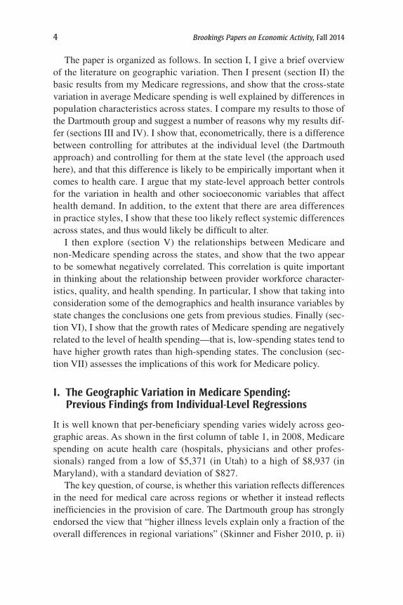
The paper is organized as follows. In section I, I give a brief overview of the literature on geographic variation. Then I present (section II) the basic results from my Medicare regressions, and show that the cross-state variation in average Medicare spending is well explained by differences in population characteristics across states. I compare my results to those of the Dartmouth group and suggest a number of reasons why my results dif-fer (sections III and IV). I show that, econometrically, there is a difference between controlling for attributes at the individual level (the Dartmouth approach) and controlling for them at the state level (the approach used here), and that this difference is likely to be empirically important when it comes to health care. I argue that my state-level approach better controls for the variation in health and other socioeconomic variables that affect health demand. In addition, to the extent that there are area differences in practice styles, I show that these too likely reflect systemic differences across states, and thus would likely be difficult to alter.
I then explore (section V) the relationships between Medicare and non-Medicare spending across the states, and show that the two appear to be somewhat negatively correlated. This correlation is quite important in thinking about the relationship between provider workforce character-istics, quality, and health spending. In particular, I show that taking into consideration some of the demographics and health insurance variables by state changes the conclusions one gets from previous studies. Finally (sec-tion VI), I show that the growth rates of Medicare spending are negatively related to the level of health spending—that is, low-spending states tend to have higher growth rates than high-spending states. The conclusion (sec-tion VII) assesses the implications of this work for Medicare policy.
I. the Geographic Variation in Medicare spending: Previous Findings from Individual-Level regressions
It is well known that per-beneficiary spending varies widely across geo-graphic areas. As shown in the first column of table 1, in 2008, Medicare spending on acute health care (hospitals, physicians and other profes-sionals) ranged from a low of $5,371 (in Utah) to a high of $8,937 (in Maryland), with a standard deviation of $827.
The key question, of course, is whether this variation reflects differences in the need for medical care across regions or whether it instead reflects inefficiencies in the provision of care. The Dartmouth group has strongly endorsed the view that “higher illness levels explain only a fraction of the overall differences in regional variations” (Skinner and Fisher 2010, p. ii)

Louise sheiner 5
and hence that most of the variation reflects inefficiencies. For example, Sutherland, Fisher, and Skinner (2009) find that controlling for age, race, income, self-reported health status, presence of diabetes, blood pressure, body-mass index, and smoking history only eliminates about 30 percent of the difference between spending in the top and bottom quintiles.3 They conclude that “more than 70% of the differences in spending . . . cannot be explained away by the claim that ‘my patients are poorer or sicker’ ” (p. 1228). Instead, their view is that the variation reflects differences in the way medicine is practiced—practice styles—and that by simply emulating the practices of the health providers in the cheaper states, care could be up to 30 percent cheaper (Fisher and others 2003).
But including only a few health measures in the equation does not allevi-ate the concern that there is still important omitted variation in underlying health needs. Other researchers have attempted to do a better job control-ling for the health of beneficiaries. For example, Stephen Zuckerman and
table 1. Cross-state Variation in Per-Beneficiary Medicare spending, Controlling for Prices, income, And Population Characteristics, 2008 In annual dollars
No controls (actuals)a
Control for income and Medicare
pricesb
Control for income,
Medicare prices, and
diabetes ratesb
Control for income, age
groups, diabetes rates, race, and
uninsuredb
Average 6,790 6,790 6,790 6,790Standard deviation 827 698 410 328Coefficient of variation
12% 10% 6% 5%
Lowest 5,371 5,580 5,798 6,055Highest 8,937 8,239 7,568 7,510Range 3,566 2,659 1,770 1,455
Source: Author’s analysis; see online appendix for data sources.a. The first column describes the distribution of per-beneficiary acute Medicare spending across
the states.b. Columns 2, 3, and 4 calculate an adjusted per-beneficiary Medicare spending for each state, equal to
the mean per-beneficiary spending plus the residual from the regression described in the column heading.
3. An additional difference is that the quintiles in the Medicare Beneficiary Survey are defined as hospital-referral regions (HRRs), rather than states. Given that there is varia-tion in spending within states, there is more variation across HRRs than across states. For example, the state data show a 29-percent difference in real spending between bottom and top quintiles, whereas the HRR data show a 52-percent difference. Thus, the state data might understate the amount of unexplained variation. On the other hand, some of the variation in HRRs is more likely to reflect random variation.

6 Brookings Papers on Economic Activity, Fall 2014
others (2010) explore the effects of adding additional health measures as controls in the estimating equations. They control for whether the indi-vidual died that year, whether a number of conditions were newly diag-nosed, and whether the individual had a history of heart attack, stroke, or any of a number of other conditions. In addition, they include information on supplementary health insurance. Including these other health factors explains an additional 7 percent of the difference between quintiles 1 and 5, so that 63 percent of the variation remains unexplained. As they note, however, even with their health measures, they “do not capture the severity of illness or the presence of multiple chronic conditions” (p. 61).
Including even more detailed measures of beneficiary health reduces the geographic variation further (MedPAC 2009), with a study by James Reschovsky, Jack Hadley, and Patrick Romano (2013) finding that dif-ferences in health explain between 75 percent and 85 percent of the geo-graphic variation in spending. However, Skinner and Fisher, both with Dartmouth, point out that the additional controls, which are garnered from the Medicare billing records, depend on doctors having diagnosed condi-tions in order to perform procedures, and may well control for the very varia-tion that they are trying to explain. They note that “regions that have doctors who do more testing will have patients with more diagnoses and thus will appear to have sicker patients” (Skinner and Fisher 2010, p. 8). This con-cern is a reasonable one (see, for example, Wennberg and others 2013), yet not adequately controlling for patient health is also highly problematic when one is trying to isolate health care spending that is not explained by patient characteristics.
The profound influence that the Dartmouth work had on the public dis-course led Congress, during its negotiations over health reform, to direct the Institute of Medicine to convene a panel of experts to grapple with the question of whether Medicare should actually use the geographic variation in health spending as a basis of payment policy—that is, whether Medicare should lower payments to high spending areas. The Institute of Medicine commissioned research that examined individual insurance claims (from Medicare, Medicaid, and private insurers) and used the information on the claims to adjust for the patients’ individual health status. The institute’s report, titled “Variation in Health Care Spending: Target Decision Making, Not Geography,” concludes that while health spending exhibited sizable and persistent variation even when it was adjusted for price and risk, it is not possible to characterize some areas as systematically overspend-ing or underspending. In particular, it notes that using a geographic adjustment would “unfairly reward low-value providers in high-value

Louise sheiner 7
regions and punish high-value providers in low-value regions” (Institute of Medicine 2013, p. 17.)
A recent paper by Amy Finkelstein, Matthew Gentzkow, and Heidi Williams (2014) analyzes the health spending of Medicare beneficiaries when they move from one area to another. The idea is that, if health spend-ing varies only because of individual health characteristics, then there should be no impact on these movers’ Medicare expenditures when they relocate from a low-spending to a high-spending area. In contrast, if health spending variation is unrelated to health, then a mover’s health spending should increase (or decrease) in direct proportion to the difference in mean health spending between the old and new locations. Using this method-ology, the authors find that, on average, about half of the difference in price-adjusted Medicare spending across areas is directly attributable to differences in individual health characteristics.
To summarize: It is clear that variation in illness levels explains some of the geographic variation in Medicare spending. The Dartmouth group’s view is that variation in illness is a minor contributor to spending variation. Other analysts conclude that variation in illness is a much more important factor, but still find large unexplained variation.
The movers study uses a natural experiment approach that is well suited to examining the direct impact of individual health characteristics on Medi-care spending. But most of the previous work on geographic variation has been cross-sectional in nature and has relied on individual-level data. That is, previous researchers, using the health records of individual Medicare beneficiaries, have regressed spending on measures of health and have identified the mean residuals either by state or by the area fixed effects as a measure of unexplainable geographic variation.
A different approach is to start with mean health expenditures by state, and then test how much the variation in spending is associated with the attributes of the states reviewed. This approach, which I apply in my analy-sis, yields quite different results.
II. Geographic Variation Using state-Level regressions
In this section I lay out the results of my state-level regressions and also compare them with previous state-level studies.
II.A. Data Used in This Study
The main data source for this analysis is the state health accounts put together by the Centers for Medicare and Medicaid research, which

8 Brookings Papers on Economic Activity, Fall 2014
provide a breakdown of total health spending across states by payer and service. These data are supplemented by a wide variety of state-level data on income, health insurance status, health behaviors, social capital, and demographics. The measures of population health are from telephone sur-veys in which people are asked basic questions about their health; these surveys represent the health of the entire adult population. (Further details on the sources for these data are included in the online appendix.4)
This study focuses on the level of “acute” health spending—that is, spending on hospitals, physicians, and other professionals—and omits spending on long-term care, dental care, and prescription drugs. Acute health spending, which accounted for 73 percent of Medicare spending in 2008, is what analysts typically have in mind when discussing physi-cian practice styles. Long-term care, which accounted for 12 percent of spending, will be driven in important ways by both social factors (such as whether seniors’ children provide care at home) and Medicaid’s nursing home policies, which vary across the states in ways unrelated to the health care system per se.5 In any case, the results for total Medicare spending are virtually identical to those for acute health spending.6
The focus on acute spending also makes comparisons between Medicare spending and spending for the non-Medicare population easier, since the non-Medicare population is much less likely to use long-term care. I use both the state health accounts and private health insurance premiums from the Medical Expenditure Panel Survey (MEPS)7 to measure non-Medicare spending. The empirical work in this paper uses data from 2008, but the results are quite similar for earlier years.
4. Online appendixes for this volume may be found at the Brookings Papers website, www.brookings.edu/bpea, under “Past Editions.”
5. Thus, these data are not subject to the criticism (raised in Skinner and others 2008) that the aggregate spending by state is affected by family support, community centers, and respite care for low-income elderly or disabled people. Nevertheless, a disadvantage of this approach is that it ignores much of post-acute care, which has become an increasingly impor-tant source of geographic variation over time.
6. The Institute of Medicine (2013) has pointed out that post-acute care—and particu-larly home health care—is the largest source of unexplained variation in spending across regions. While my regressions for total spending and for acute spending are virtually identi-cal, I too find that when running regressions component by component I am able to explain only about 50 percent of the variation in nonacute care. MedPac (2011) has suggested that there is evidence of fraud in the use of home health services and durable medical equipment in Medicare; such variation could be significantly reduced by antifraud measures.
7. The Medical Expenditure Panel Survey, which began in 1996, is an annual survey of households and employers that gathers information on medical usage, costs, and health insurance. It is sponsored by the Agency for Healthcare Research and Quality.
Louise sheiner 9
II.B. Results from State-Level Regressions
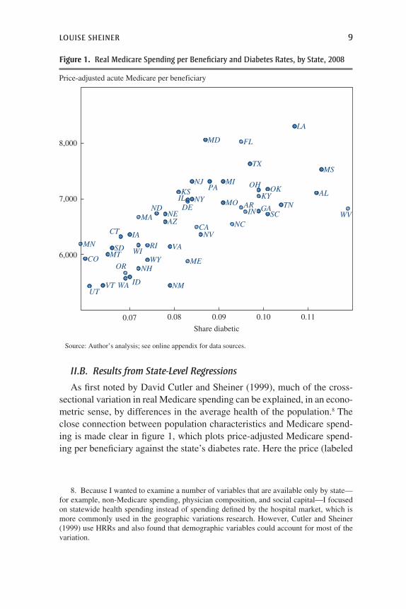
As first noted by David Cutler and Sheiner (1999), much of the cross-sectional variation in real Medicare spending can be explained, in an econo-metric sense, by differences in the average health of the population.8 The close connection between population characteristics and Medicare spend-ing is made clear in figure 1, which plots price-adjusted Medicare spend-ing per beneficiary against the state’s diabetes rate. Here the price (labeled
8. Because I wanted to examine a number of variables that are available only by state—for example, non-Medicare spending, physician composition, and social capital—I focused on statewide health spending instead of spending defined by the hospital market, which is more commonly used in the geographic variations research. However, Cutler and Sheiner (1999) use HRRs and also found that demographic variables could account for most of the variation.
AL
AR
AZCA
CO
CT
DE
FL
GA
IA
ID
IL
IN
KS KY
LA
MA
MD
ME
MI
MN
MO
MS
MT
NC
NDNE
NH
NJ
NM
NV
NY
OH OK
OR
PA
RI
SC
SD
TN
TX
UT
VA
VT WA
WI
WV
WY6,000
7,000
8,000
0.07 0.08 0.09 0.10 0.11
Share diabetic
Price-adjusted acute Medicare per beneficiary
Source: Author’s analysis; see online appendix for data sources.
Figure 1. real Medicare spending per Beneficiary and Diabetes rates, by state, 2008

10 Brookings Papers on Economic Activity, Fall 2014
“Medicare price” in the following tables) reflects the average geographic adjustment used by Medicare to compensate providers in different areas.9
Table 2 reports the results of regressions of the log of per-beneficiary acute Medicare spending on state characteristics. As shown in column 1, per capita income explains only about 15 percent of the variation in acute Medicare spending across states. Adding in the Medicare price (column 2) boosts the explanatory power to just 22 percent.10 However,
9. Medicare adjusts payments to providers for differences in local wage rates, teaching hospital status, and the degree of uncompensated care. I use the ratio of actual to price-standardized Medicare payments for services as the price measure, excluding skilled nurs-ing facilities, home health, hospice, and durable medical equipment. See CMS Geographic Variation Public Use Files (https://www.cms.gov/Research-Statistics-Data-and-Systems/Statistics-Trends-and-Reports/Medicare-Geographic-Variation/GV_PUF.html).
10. The coefficient on the log of the Medicare price variable is less than 1, meaning that a 1-percent increase in provider compensation raises Medicare spending by less than 1 percent. This may be because the price is measured with error (the categories used in the Medicare files from which it is gathered do not match the categories in the state health accounts exactly) or, more likely, because the variable is picking up something about the characteristics of the population.
table 2. regressions identifying effect of state Characteristics on Cross-state Medicare spending Variations, 2008
Independent variable
Dependent variable: Log acute Medicare spending per beneficiary by state, 2008a
(1) (2) (3) (4)
Log per capita income 0.35**(0.11)
0.13(0.15)
0.44**(0.09)
0.31**(0.09)
Log Medicare price 0.64**(0.29)
0.65**(0.17)
0.72**(0.14)
Percent diabetic 6.3**(0.70)
4.5**(0.81)
Percent black 0.43**(0.12)
Percent uninsured 0.47*(0.24)
Share elderly (ages 65–74) -1.6**(0.37)
Constant -1.8(1.2)
0.55(1.5)
-3.2**(1.0)
-1.1(1.0)
No. of observations 48 48 48 48Adjusted R2 0.15 0.22 0.72 0.81
Source: Author’s analysis; see online appendix for data sources.a. Statistical significance at the *10 and **5 percent levels.

Louise sheiner 11
simply including a state’s diabetes rate increases the explained share of spending to 72 percent, which is not surprising given the results in figure 1. The coefficient on diabetes (6.3) suggests that an increase in diabetes incidence in adults from 6 percent to 12 percent (0.06 to 0.12)—which are the rates in Minnesota and West Virginia, respectively—would increase Medicare expenditures by almost 40 percent. Notice that the increase in the R2 of the equation from the inclusion of a state’s diabetes rate—about 50 percentage points—mirrors the share of variation associ-ated with health characteristics that was found in the study of movers (Finkelstein and others 2011) discussed above.11
As shown in column 4, spending is higher when more of the population is uninsured and black, and it is lower the greater is the share of 65- to 74-year-olds in the elderly population. With all these variables included in the regression, the R2 increases to 81 percent. Thus, most of the geo-graphic variation in Medicare spending across the states is explainable in an econometric sense by some simple measures of population characteristics.
Turning back to table 1, one can see how the variation in health spend-ing changes once these factors are accounted for. As the far-right column there shows, including age, income, health, and other demographic factors lowers the standard deviation from $827 for the unadjusted spending to just $328 for the adjusted spending. Figure 2 plots the adjusted Medicare spending (in logs) against the log of unadjusted Medicare. It shows that, while adjusted and unadjusted spending are correlated, the relationship is fairly weak (the coefficient on unadjusted Medicare spending is 0.16 and the R2 is 0.15). Many states that appear to be high-cost, like New York and New Jersey, are no longer high-cost once the price, demographic, and health variables are included; similarly, Colorado and Montana, which are on the low end of the distribution of unadjusted Medicare spending, appear to be relatively high spenders once the adjustments have been taken into account. These regression results suggest that the cross-state variation in Medicare spending is tightly associated with the characteristics of state populations and that once those characteristics are controlled for the varia-tion in spending is fairly small.
Table 3 presents the information in a way that is more directly compa-rable to some of the work that has been done previously.12 For this table,
11. A more direct comparison is from a univariate regression of price-adjusted Medicare spending on diabetes; that regression has an R2 of 48 percent, also right in line with the findings of Finkelstein and others (2011).
12. For example, Zuckerman and others (2010) examined how the fixed-effects coef-ficients on spending quintiles change as more individual health variables are added.

12 Brookings Papers on Economic Activity, Fall 2014
Log actual Medicare spending
Unexplained log Medicare spendinga
8.7
8.8
8.9
9.0
8.7 8.8 8.9 9.0
AL
AR
AZ
CA
CO
CT
DEFL
GA
IAID ILIN
KS
KY
LAMA
MD
ME
MI
MN
MO
MS
MT
NCND
NE
NH
NJ
NM
NV
NY
OHOKOR
PA
RISC
SD TN
TXUT
VA
VT
WA
WI
WV
WY
Source: Author’s analysis; see online appendix for data sources.a. Unexplained log Medicare spending is the residual for each state from the regression in table 2,
column 4.
Figure 2. Adjusted and unadjusted Medicare spending, by state, 2008
table 3. Medicare spending per Beneficiary, unadjusted and Adjusted, by Quintile, 2008 Annual dollars
Quintilea
Unadjusted Medicare spending per beneficiaryb
Adjusted Medicare spending per beneficiaryc
1d 6,082 6,6162e 6,743 6,8023f 7,247 6,7814g 7,750 6,9885h 8,513 6,964
Difference quintiles 5 and 1 2,431 348
Source: Author’s analysis; see online appendix for data sources.a. Each quintile represents roughly 20 percent of the Medicare population.b. Actual acute Medicare spending per beneficiary.c. Adjusted Medicare spending equals the average Medicare spending for the entire population plus the
unexplained portion of the spending from the regression in table 2, column 4.d. UT, ID, NM, MT, WY, SD, ME, OR, VT, WA, CO, VA, IA, NH, ND, WI, AR, MN, WV, AZ.e. TN, IN, NC, SC, KS, MO, OK, GA, NV, AZ.f. KY, RI, MS, OH, IL, DE, PA, CT.g. TX, MA, MI, LA, CA.h. FL, NY, NJ, MD.

Louise sheiner 13
states are sorted according to unadjusted Medicare spending and then put into quintiles based on population shares (so that roughly 20 percent of the Medicare population is in each quintile.) The table shows how much of the variation in spending is explained by the covariates in table 2. Comparing the top quintile to the bottom quintile, one can see that unadjusted spending is $2,431, or 40 percent higher, in the top quintile compared to the bottom quintile. Adjusted spending, however, shows much less of a variance, with the difference between the top and bottom quintiles averaging just $348, or 5 percent.
These regressions show that there is a systematic relationship between population characteristics and real per-beneficiary Medicare spending: states with similar demographic characteristics have similar levels of real spending.13 Thus, what the Dartmouth researchers have deemed to be dif-ferences in “practice styles” are not randomly distributed, but are instead closely linked to population characteristics. If it had turned out that places with similar demographics—say, Kentucky and Louisiana—had widely varying spending levels, it would be easier to argue that the differences are unrelated to health needs and likely reflect provider behavior.
III. Why Are the results so Different?
The basic difference between the regressions in this paper and those used by other researchers is the level at which the health attributes are controlled for. Prior researchers have used individual health records to regress spend-ing on measures of an individual’s health, and then calculated the mean residuals by area from that regression or else run regressions with area fixed effects. My work regresses average health spending by state against average health attributes in the state and then examines the residuals from these regressions.
Although one might have expected these approaches to yield similar answers, they do not. For example, consider again the impact of diabetes on health spending. Sutherland, Fisher, and Skinner (2010) include a per-son’s body-mass index as well as the presence of diabetes and a number
13. Thus, Atul Gawande’s characterization of the two towns in Texas—El Paso and McAllen—as having similar demographics but sharply different levels of Medicare spend-ing, does not characterize the variation in spending overall (Gawande 2009). In fact, it also overstates the similarities between El Paso and McAllen: in 2007, the adult diabetes rate was 9.7 percent in El Paso County but 13.3 percent in Hidalgo County (the county McAllen is in) (Texas Department of State Health Services 2008).

14 Brookings Papers on Economic Activity, Fall 2014
of health attributes in their individual regression, which nevertheless explained only 20 percent of the variation between the top and bottom quintiles of health spending. In my state regressions, by contrast, simply including the mean obesity rate by state is sufficient to explain almost 70 percent of the health spending variation. A key question is how to inter-pret this difference.
III.A. Reasons Why the State and Individual Results Might Differ
hyPothesis 1: THE STATE REGRESSIOnS DO A BETTER jOB Of COnTROLLInG
fOR DIffEREnCES In PATIEnT HEALTH. There are two reasons why state-level variables might control better for health. First, the health and demo-graphic variables used in the state-level regressions are not exactly the same as those that are used in the individual regressions. In particular, the state-level health variables measure the average health of the entire adult population, rather than that of Medicare beneficiaries alone. Thus, state-level variables might capture conditions that have prevailed throughout a person’s life. For example, although sick patients are typically not obese, if they have been obese throughout their life that condition would be likely to contribute to their current health status. Similarly, the health costs of diabetes depend on when a person first acquired the disease; in states where the incidence of diabetes is high (generally the states where obesity is also high), diabetic Medicare beneficiaries are likely to be in worse health, on average, than diabetic beneficiaries in states where the incidence of diabetes is low. Similarly, all Medicare beneficiaries have insurance, but patients who did not have insurance prior to becoming eli-gible for Medicare are likely to be in worse health and to have a greater need for health services. Thus, the average rate of insurance in a state may be a useful marker for patient health, even for those currently with insurance.
Second, and probably more importantly, the state regressions might do a better job of picking up unobserved health. Observed and unobserved health will be correlated at the individual level if people who are in poor health in some dimensions also tend to be in poor health in other dimen-sions. For example, someone who smoked when she was younger (unob-served) may be more likely to be diabetic when older (observed). Observed and unobserved health could be further correlated at the state level if there is a third factor—say, the average stress level in a state—that affects both observed and unobserved health independently. For example, some people in states where life is more stressful may respond to the stress by smok-ing, others may respond by overeating and becoming diabetic, and others

Louise sheiner 15
may respond by both overeating and smoking. Thus, in states with a high level of smoking, both smokers and nonsmokers may be more likely to be diabetic than in states with lower smoking levels. If this is the case, the average diabetes level in a state will tell more about unobserved smoking behavior than measures of whether an individual is diabetic.
hyPothesis 2: PRACTICE STyLES ARE GEARED TOWARD THE HEALTH Of THE
TyPICAL PATIEnT, WHICH IS OnLy MEASURABLE In THE STATE-LEVEL REGRESSIOnS. A second hypothesis is that health systems may be geared toward the median or average patient. Physicians practicing in states with a sicker population may practice a more intensive form of medicine for all their patients than those practicing in states with a healthier population. For example, in states with sicker populations, hospitals may be more likely to invest in new technologies and physicians may be more likely to adopt more invasive procedures. Under this hypothesis, it is the mean level of health needs that will determine medical expenditures, rather than the individual level, so an approach based on state means will do a better job of capturing the link between population health and Medicare expenditures.
hyPothesis 3: PROVIDERS EnGAGE In “VOLUME SHIfTInG.”14 Previous research has shown that health providers respond to financial incentives (Jacobson and others 2006, Clemens and Gottlieb 2012, Hadley and Reschovsky 2006). Providers might practice a more intensive form of medicine, or just bill Medicare more for similar care, in places where the nonelderly popu-lation is uninsured or underinsured or where private reimbursement rates are low. While such shifting may not be the most efficient mechanism to finance health care, it also suggests that the Medicare expenditures could not be reduced without adverse effects on the health system.
hyPothesis 4: SOCIAL CAPITAL AffECTS PROVIDER BEHAVIOR. The Dartmouth researchers suggest that the strong correlation between states’ attributes and spending may be due to differences in social capital that directly affect provider behavior.15 Skinner and others (2008) note that “physicians who
14. In the health economics literature, cost shifting is defined as the situation in which, in response to cuts in the level of public program reimbursements, providers are able to raise the prices paid by those with insurance. A second possible response—“volume shifting”—occurs when providers shift resources away from those with public insurance and toward those with private insurance. See Rice and others (1999) and Showalter (1997).
15. Social capital is a measure of social cohesion created by Robert Putnam, author of Bowling Alone: The Collapse and Revival of American Community (Putnam 2000). It is an agglomeration of responses to questions related to community involvement (voting, PTA attendance) and levels of trust (answers to questions such as “Are people generally trustworthy?”).

16 Brookings Papers on Economic Activity, Fall 2014
live in . . . high social-capital states are more likely to adopt new and effec-tive innovations rather than simply performing more tests and procedures with questionable medical efficacy” (p. 122). Work by Skinner and Staiger (2007) demonstrates that states with high levels of social capital are more likely to follow recommended guidelines about prescribing beta blockers in the treatment of heart attacks. Because the choices made by physicians seem the most easy to influence, this hypothesis suggests that it might be possible to devise Medicare policies that would reduce geographic varia-tion and yield savings for the Medicare system. On the other hand, to the extent that poor social capital affects the quality of the providers and their staffs, finding such policies might be quite challenging.
III.B. A formal Comparison of Individual and State-Level Regressions
It is helpful to write down a simple model to clarify the sources of dif-ferences between state- and individual-level regressions. In the following, assume that samples are infinite, so sample means are equal to population means. Let i index individuals and j index states. Let eH
ij, eUij, and eO
ij be mean-zero individual-level random variables that are independent across individuals, independent of each other, and independent of all state-level random variables. Similarly, let wU
–
j and wjP be mean-zero state-level ran-
dom variables that are independent across states and independent of each other.
The health spending of individual i living in state j, denoted Hij, is a function of observed health, Oij, unobserved health, Uij, the state practice style, Pj, and random error eH
ij:
H O U Pij ij ij j ijH(1) .= α + β + γ + + ε
Assume that health conditions are measured such that higher levels increase health spending, so b and g are both positive.
An individual’s observed health is equal to the mean observed health in a state plus a random error term:
O Oij j ijO(2) .= + ε
reLAtionshiP Between oBserVeD AnD unoBserVeD heALth. An individ-ual’s unobserved health is related to both the individual’s own observed health and the mean unobserved health in that person’s state. In particular, Uij is equal to the mean unobserved health in the state, U
–j, plus d times the

Louise sheiner 17
difference between the individual’s and the state-mean observed health, (Oij - O
–j) and a random error eU
ij:16
U U O Oij j ij j ijU( )= + δ − + ε(3) .
The relationship between unobserved and observed health at the indi-vidual level also translates into a relationship at the state level. That is, if people with poor observed health also have poor unobserved health, then states with a lot of people with poor observed health will necessarily have a lot of people with poor unobserved health. This relationship is captured by the coefficient d. There is also an additional state-level relationship between mean observed health O
–j and unobserved health, U
–j, measured by
the coefficient z, such that mean unobserved health in a state is:
U z Oj j jU(4) .( )= + δ + ω
The coefficient z captures the relationship between observed and unob-served health that occurs only at the state level. That is, it captures the pos-sibility, raised by hypothesis 1 above, that for an individual with a given observed health, his or her unobserved health is likely to be worse if he or she is in a less healthy state. If no such relationship exists, then z = 0. Combining equations 2 and 3, individual unobserved health can be rewrit-ten this way:
= δ + + ω + ε(5) .U O zOij ij j jU
ijU
PrACtiCe styLes. As described above, there are a number of reasons why practice styles might be related to mean health in a state: because physi-cians practice the type of medicine that works best for the median patient (hypothesis 2); because poor-health states are also under-resourced states, and providers volume-shift (hypothesis 3); because poor-health states are states with low social capital, and providers make worse choices when social capital is low (hypothesis 4).
For ease of exposition, assume that practice styles are only a function of observable (rather than observable and unobservable) health characteristics:
= + ω(6) .P xOj j jP
16. The subtraction of mean observed health in the Oij - O–
j term is necessary in order for the mean of the left-hand side of equation 3 to equal mean unobserved health in the state.
18 Brookings Papers on Economic Activity, Fall 2014
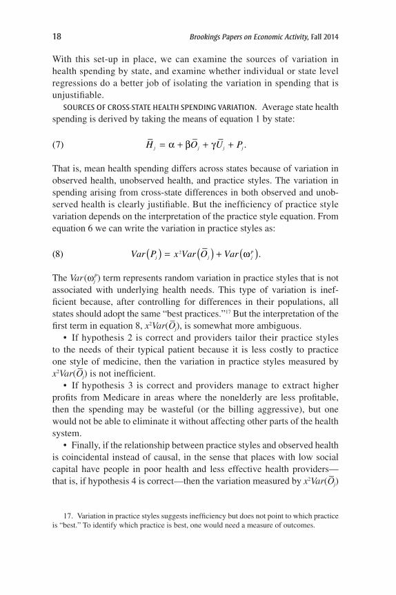
With this set-up in place, we can examine the sources of variation in health spending by state, and examine whether individual or state level regressions do a better job of isolating the variation in spending that is unjustifiable.
sourCes oF Cross-stAte heALth sPenDing VAriAtion. Average state health spending is derived by taking the means of equation 1 by state:
= α + β + γ +(7) .H O U Pj j j j
That is, mean health spending differs across states because of variation in observed health, unobserved health, and practice styles. The variation in spending arising from cross-state differences in both observed and unob-served health is clearly justifiable. But the inefficiency of practice style variation depends on the interpretation of the practice style equation. From equation 6 we can write the variation in practice styles as:
Var P x Var O Varj j jP(8) .2 ( )( ) ( )= + ω
The Var(wjP) term represents random variation in practice styles that is not
associated with underlying health needs. This type of variation is inef-ficient because, after controlling for differences in their populations, all states should adopt the same “best practices.”17 But the interpretation of the first term in equation 8, x2Var(O
–j), is somewhat more ambiguous.
• If hypothesis 2 is correct and providers tailor their practice styles to the needs of their typical patient because it is less costly to practice one style of medicine, then the variation in practice styles measured by x2Var(O
–j) is not inefficient.
• If hypothesis 3 is correct and providers manage to extract higher profits from Medicare in areas where the nonelderly are less profitable, then the spending may be wasteful (or the billing aggressive), but one would not be able to eliminate it without affecting other parts of the health system.
• Finally, if the relationship between practice styles and observed health is coincidental instead of causal, in the sense that places with low social capital have people in poor health and less effective health providers—that is, if hypothesis 4 is correct—then the variation measured by x2Var(O
–j)
17. Variation in practice styles suggests inefficiency but does not point to which practice is “best.” To identify which practice is best, one would need a measure of outcomes.

Louise sheiner 19
measures inefficient provider practices. This hypothesis, if true, is consis-tent with the Dartmouth view that some places practice better and more efficient medicine than others. But, even assuming that this hypothesis is correct, the fact that there are systematic differences between places that practice good medicine and places that do not suggests that improving efficiency will be no easy task.
We can now examine how well individual and state level regressions account for the cross-state variation in Medicare spending.
inDiViDuAL-LeVeL regressions. Some research (such as Institute of Medicine 2013) corrects for differences in health spending by estimat-ing national regressions of health spending on health characteristics, and then calculating the residuals by geographic area. Other work (Zuckerman and others 2010) runs national regressions with fixed effects to calculate the unexplained variation by geographic area. Both are considered below:
An individual-level regression of health spending on observed health attributes can be written as
H a b O eijind ind
ij ijind(9) ˆ ˆ ˆ .= + +
If we rewrite equation 1 in terms of observed health, we see that
H O U P
O zO O xO
O z x O
ij ij ij j ijH
ij j ij jU
ijU
j jP
ijH
ij j jU
ijU
jP
ijH
(10)
.[ ]( )
( ) ( )
= α + β + γ + + ε
= α + β + γ + δ + ω + ε + + ω + ε
= α + β + γδ + γ + + γω + γε + ω + ε
Note that, through equations 3, 4, and 6, the error in the square brackets in equation 10 is correlated with Oij, which means that b̂ind is a biased and inconsistent estimator of both b and b + gd. In particular,
bCov H O
Var O
Var O
Var Oz x
m z x
ind ij ij
ij
j
ij
(11) ˆ ,
,
( )( )( ) ( )( ) ( )
( ) ( )
= = β + γδ + γ +
= β + γδ + γ +
where m is the ratio of the variances of state-mean observed health to indi-vidual observed health. Given that observed health varies within a state as well as across states (from equation 6: Oij = O
–j + eO
ij), we know that m < 1.

20 Brookings Papers on Economic Activity, Fall 2014
With a fixed-effects regression, the coefficient on the state dummy will capture all the variation by state that is not captured by observed health. In particular, Dj, the coefficient on the dummy variable in state j, will be
( )= γ + + γω + ωD z x Oj j jU
jP .
The coefficient on observed health, b̂ind,FE, will be
bCov H O
Var Oind FE ij ij
ij
(12) ˆ ,.,
( )( ) ( )= = β + γδ
stAte-LeVeL regression. Taking means by state from equations 1 and 5, we can write
( )( )= α + β + γ δ + + + γω + ωH z x Oj j jU
jP(13) .
Because wjU– and wj
P are both mean-zero and independent of all other random variables, the error in this regression does not covary with the independent variable. Thus, in the following state-level regression:
= + +H a b O ejstate state
j jstate(14) ˆ ˆ ˆ ,
the estimated coefficient on mean observed health is simply
( )( )= β + γ δ + +(15) ˆ .b z xstate
CoMPAring stAte AnD inDiViDuAL-LeVeL regressions. Why can the state-level regressions explain so much more of the cross-state regressions than the individual-level regressions, and which regression correctly character-izes the degree of inefficiency in the Medicare system?
The residuals from an individual-level regression of health spending on observed health are
e H H b O Oijind
ijind
ij(16) ˆ ˆ ,( )( )= − − −
so the mean residuals by state are
( )( )= − − −e H H b O Ojind
jind
j(17) ˆ ˆ .

Louise sheiner 21
Similarly, the residuals from the state regressions of mean health spending on mean observed health are
( )( )= − − −e H H b O Ojstate
jstate
j(18) ˆ ˆ .
The only way for the residuals to differ is if the individual and state-level regressions produce different coefficients on observed health. Index the three types of regressions by k, where k can be (i) the individual regression without fixed effects; (ii) the individual fixed-effects regression; or (iii) the state-level regression. Then, note that all three coefficients can be written as
( ) ( )= β + γδ + γ +b K z xkˆ .
When k refers to the individual regression without fixed effects, K = m, the ratio of the variance of state-mean observed health to the variance of individual observed health, which is positive but less than 1. When k refers to the fixed-effects regression, K = 0, and when k refers to the state-level regression, K = 1.
So b̂ind, b̂ind,FE, and b̂state will differ if:(i) gz > 0: There is a state-specific factor, like stress, that affects both
observed and unobserved health independently (hypothesis 1)and/or(ii) x > 0: Physician practice styles depend on the mean health of the
area (hypotheses 2 through 4).In both of these cases, the coefficient on observed health will be larger in
the state regressions, and the unexplained variation will be smaller.Figure 3 provides the simple intuition for this result. In the top panel,
observed health varies both within and across states 1, 2, and 3. As the mea-sure of observed health (health problems) increases, so too does individual health spending. However, in addition, holding individual observed health constant, states with higher average measures of observed health have higher spending. Under this assumption (and with just three data points), the state-level regression will perfectly predict health spending, and state residuals will be zero. The individual regression line is flatter, however, and the regression over-predicts spending for state 1 and under-predicts it for state 2. With an individual fixed-effects regression, the slope of the regression line is equal to the slope within a state. All of the difference in spending that is not directly associated with observed illness is captured by the state fixed effect.

22 Brookings Papers on Economic Activity, Fall 2014
Health spending
Observed health
Health spending
Observed health
1 1 11 1 1 11 1 1 1 11 1 1 11 1 1 11 1 1 1 11 1 1 11
2 2 2 22 2 2 22 2 2 2 22 2 2 22 2 2 22 2 2 2 22 2 2 2
33 3 3 33 3 3 33 3 3 3 33 3 3 33 3 3 33 3 3 3 33 3 3
111111111111111111111111111111
222222222222222222222222222222
333333333333333333333333333333
4
5
6
7
8
1.0 1.5 2.0 2.5 3.0
Individual observationsMeans by stateIndividual regression lineState regression line
1 1 1 1 1 1 1 1 1 1 1 1 1 1 1 1 1 1 1 1 1 1 1 1 1 1 1 1 1 1
2 2 2 2 2 2 2 2 2 2 2 2 2 2 2 2 2 2 2 2 2 2 2 2 2 2 2 2 2 2
3 3 3 3 3 3 3 3 3 3 3 3 3 3 3 3 3 3 3 3 3 3 3 3 3 3 3 3 3 3
1.2
1.4
1.6
1.8
0.5 1.0 1.5 2.0
Individual observationsMeans by stateIndividual and state regression line
Source: Author’s analysis; see online appendix for data sources.
Figure 3. intuitive Model of relationship between health spending and observed health in three Fictional states, individual vs. state regressions

Louise sheiner 23
In contrast, the bottom panel shows that if practice styles are invariant to health and there is no unobserved illness, individual and state regres-sion lines are the same and the state regressions would have no additional explanatory power.
unexPLAineD VAriAtion in heALth sPenDing. The health spending that is “unexplained” by illness is
( )( )
( )( ) ( )
= − − −
= γ + − − + γω + ω
e H H b O O
z x O O K
jk
jk
j
j jU
jP
(19) ˆ ˆ
1 .
Thus, the smaller K is, the larger is the “unexplained” variation in health spending. Because K = 0 in the individual fixed-effects regression and is likely close to 0 in the individual-level regression without fixed effects, the state regression will “explain” much more of the variation in health spending.
With the state-level regression, K = 1, so each state’s regression error is simply
ejstate
jU
jP(20) ˆ .= γω + ω
It is easy to show which sources of variation are “unexplained” by the individual regressions but “explained” by the state regressions. These are:
(i) a fraction (1 - K) of the component of unobserved health that is correlated with mean observed health; and
(ii) a fraction (1 - K) of the component of practice styles that is cor-related with mean observed health.
As already discussed, health spending that varies because of unobserved health is unambiguously justifiable.18 If practice styles reflect the mean health in an area because it is economically efficient to use them, then the state-level regressions will also do a better job of identifying “inefficient” spending than the individual regressions will. Only if practice styles reflect mean health—in a way that is more coincidental than causal—could the case be made that the individual-level regressions provide a better mea-sure of the inefficient variation in health spending. Hypothesis 4, which
18. Such spending is not efficient in any large sense because it is not easy to justify dif-ferent parts of the population having such large differences in health status. But, given that they do, it is certainly justifiable that Medicare will spend more.
24 Brookings Papers on Economic Activity, Fall 2014
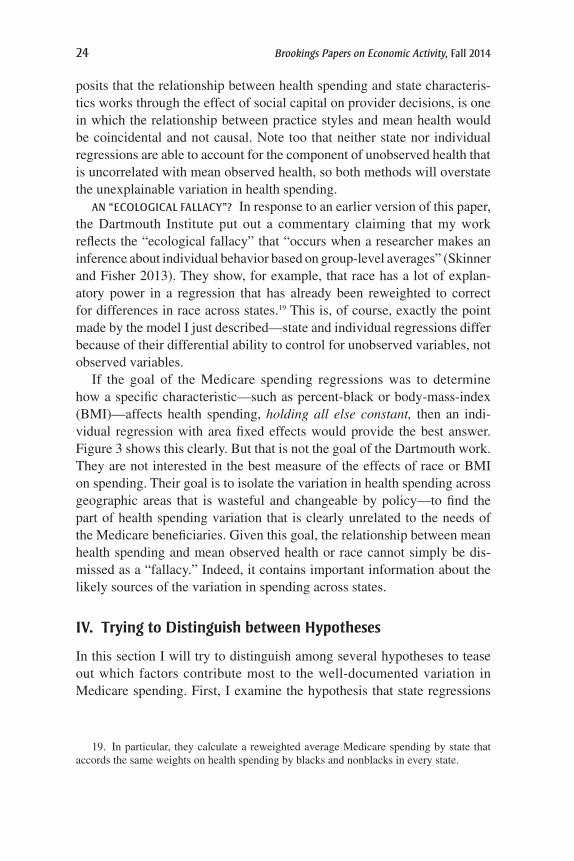
posits that the relationship between health spending and state characteris-tics works through the effect of social capital on provider decisions, is one in which the relationship between practice styles and mean health would be coincidental and not causal. Note too that neither state nor individual regressions are able to account for the component of unobserved health that is uncorrelated with mean observed health, so both methods will overstate the unexplainable variation in health spending.
An “eCoLogiCAL FALLACy”? In response to an earlier version of this paper, the Dartmouth Institute put out a commentary claiming that my work reflects the “ecological fallacy” that “occurs when a researcher makes an inference about individual behavior based on group-level averages” (Skinner and Fisher 2013). They show, for example, that race has a lot of explan-atory power in a regression that has already been reweighted to correct for differences in race across states.19 This is, of course, exactly the point made by the model I just described—state and individual regressions differ because of their differential ability to control for unobserved variables, not observed variables.
If the goal of the Medicare spending regressions was to determine how a specific characteristic—such as percent-black or body-mass-index (BMI)—affects health spending, holding all else constant, then an indi-vidual regression with area fixed effects would provide the best answer. Figure 3 shows this clearly. But that is not the goal of the Dartmouth work. They are not interested in the best measure of the effects of race or BMI on spending. Their goal is to isolate the variation in health spending across geographic areas that is wasteful and changeable by policy—to find the part of health spending variation that is clearly unrelated to the needs of the Medicare beneficiaries. Given this goal, the relationship between mean health spending and mean observed health or race cannot simply be dis-missed as a “fallacy.” Indeed, it contains important information about the likely sources of the variation in spending across states.
IV. trying to Distinguish between Hypotheses
In this section I will try to distinguish among several hypotheses to tease out which factors contribute most to the well-documented variation in Medicare spending. First, I examine the hypothesis that state regressions
19. In particular, they calculate a reweighted average Medicare spending by state that accords the same weights on health spending by blacks and nonblacks in every state.

Louise sheiner 25
do a better job than individual regressions of picking up unobserved health characteristics, in case it is these unobserved characteristics that explain most of the variation. Second, I test the hypothesis that physicians prac-tice more efficient medicine where social capital is higher. Third, I test the hypothesis that in areas with low levels of Medicare spending, physicians are more likely to choose less aggressive treatment options whenever a medical consensus is lacking. Finally, I examine the general hypothesis that geographic variation in spending reflects different practice styles at all, by looking to see if there is similar variation in spending for non-Medicare patients, all else held equal.
IV.A. Covariance in Health Measures across States
The hypothesis that the state regressions do a better job of picking up unobserved health is one that relies on health variables being more cor-related at the state level than at the individual level. I test this hypothesis with data from the Behavioral Risk Factor Surveillance System (BRFSS), a telephone survey that asks about regular exercise, smoking, diabetes, obe-sity, self-reported health, and insurance status.20 An advantage of these data is that, unlike the health variables from the Medicare billing records, they represent basic measures of health. As a result, they should be unaffected by the practice styles of the individuals’ health providers.
Table 4 compares the coefficients from state and individual-level bivari-ate regressions of five measures of health or health behaviors: regular exer-cise, smoking, obesity, diabetes, and self-reported health. The top panel shows the results when regressions are run on individuals; the bottom panel shows the results when the regressions are of state means (of the identical data). State-level health measures are much more highly correlated than individual health measures. For example, the mean smoking rate in a state is a much better predictor of mean health status than an individual’s smok-ing is of his or her health status. A 1-percentage-point increase in the rate of smoking in a state is associated with a 0.3-percentage-point increase in the mean rate of poor health in a state; whereas at the individual level, a 1-percentage-point increase in the smoking rate raises the likelihood of poor health by only 0.02 percent. This discrepancy suggests that the state-level
20. The BRFSS is a very large telephone survey about risk behaviors, preventive health practices, and health conducted annually by state health departments in conjunction with the Centers for Disease Control and Prevention.

26 Brookings Papers on Economic Activity, Fall 2014
health regressions are likely to do a better job of picking up omitted health variables than the individual-level regressions.
Consider a data set that had information on an individual’s exercise, smoking, poor health, diabetes, and insurance status, but not on obesity. How much better would state-level means of these variables be at explain-ing cross-state variation in self-reported health status than individual-level regressions? As shown in table 5, the answer is: much better. The table com-pares the following methodologies. First, the “individual-level” approach uses the micro data to regress individual characteristics on the dependent variable. For example, in the first row of the table, the dependent variable is obesity and the independent variables are age, sex, smoking, health status, diabetes incidence, and insurance status. I then calculate the mean residual of these regressions by state. This is similar to what Dartmouth does when it calculates the residuals of age-, sex-, and illness-adjusted spending by state. The R2 in the table is simply equal to 1 minus the ratio of the variance of the mean residuals divided by the variance of the mean obesity rates
table 4. Bivariate regressions of health Measures, individual vs. state Means
Regressions of individual data (N = 178,698)
Dependent variable
Independent variablePoor
healthCurrent smoker
Exercise regularly Obese Diabetes
Poor health 0.07 -0.12 0.13 0.21Current smoker 0.02 -0.05 -0.04 -0.02Exercise regularly -0.03 -0.06 0.07 -0.01Obese 0.03 -0.05 -0.08 0.09Diabetes 0.15 -0.06 -0.04 0.26
Regressions of state means (N = 51)
Dependent variable
Independent variablePoor
healthCurrent smoker
Exercise regularly Obese Diabetes
Poor health 0.86 -1.22 0.77 0.39Current smoker 0.34 -0.56 0.39 0.15Exercise regularly -0.31 -0.35 -0.36 -0.16Obese 0.45 0.58 -0.82 0.3Diabetes 1.1 1.1 -1.9 1.48
Source: Author’s analysis of Behavioral Risk Factor Surveillance Data, 2000.

Louise sheiner 27
across the states. It measures the share of the cross-state variation that is eliminated once the individual health attributes are controlled for.21
The table shows that, in general, the state-level regressions have much more power than the individual-level regressions. For example, as shown in row 1, controlling for individual health variables other than obesity reduces the variance in mean obesity across states by 24 percent, whereas the state-level regression (where mean obesity is regressed against the means of the other health variables) explains 61 percent of the variance across states. This pattern holds regardless of which health variable is omitted. For example, while controlling for individual health attributes does nothing to explain the cross-state variation in smoking, including the state means of those variables explains 45 percent of it. (This is not surprising given that, at the individual level, smoking is negatively correlated with obesity and diabetes.) Similarly, the explained share of the cross-state variation in the exercise increases from 17 percent to 58 percent, and the explained share
table 5. regressions of health Measures on Variation in spending, Comparing individual-Level and state-Level Approaches
Dependent variable Independent variables
Share of state variation explained
(1) Individual-level
regressions
(2) State-level regressions
1. Obesity Smoker, poor health, sedentary, diabetic, insurance status, age, sex
0.24 0.61
2. Smoker Poor health, obesity, sedentary, diabetic, insurance status, age, sex
0.01 0.45
3. Poor health Obesity, smoker, sedentary, diabetic, insurance status, age, sex
0.30 0.74
4. Sedentary Obesity, smoker, poor health, diabetic, insurance status, age, sex
0.16 0.58
5. Diabetes Smoker, poor health, sedentary, obesity, insurance status, age, sex
0.47 0.63
Source: Author’s analysis of Behavioral Risk Factor Surveillance Data, 2000.
21. Note that the numbers in the table are not the R2 of the individual-level regressions. These variables may explain little of the variation in the dependent variable across individu-als (for example, if much of the variation is random) but do a much better job accounting for the differences across states (where random variation is mostly eliminated).

28 Brookings Papers on Economic Activity, Fall 2014
of self-reported poor health increases from 30 percent to 74 percent, when going from individual-level to state-level regressions.
These regressions suggest that mean health variables will do an excel-lent job of characterizing the health status of a population—much better than including a few measures of individual health. Of course, as more and more individual health variables are included at the individual level, unobserved health becomes much less of an issue. The problem with this approach, as Skinner and Fisher (2010) point out (correctly, I think), is that it becomes hard to distinguish between an individual’s actual underlying health and the health codes that appear on charts of patients for whom pro-cedures have been ordered.
IV.B. Testing the Importance of Social Capital
As noted above, Skinner and others (2009) hypothesize that physicians practice more efficient medicine where social capital is higher. Accord-ing to Putnam (1995), social capital represents “features of social life—networks, norms, and trust—that enable participants to act together more effectively to pursue shared objectives” (pp. 664–65). Research has consis-tently found it to be associated with a wide range of economic and political outcomes (Glaeser and others 1999), including health outcomes and health behaviors.22
In the following, I use the measure of social capital put together by Putnam, just as Skinner and Fisher do.23 Figure 4 shows that social capital is indeed correlated with price-adjusted Medicare spending per beneficiary. However, social capital is also highly correlated with many other attributes of communities that are likely to affect health spending. Figure 5 shows the remarkable correlations between a state’s level of social capital and, first, its diabetes rate (top panel) and, second, its black percentage of the population (bottom panel). Thus, it is possible that the association between social capital and Medicare spending is simply picking up the relationship between population health and Medicare spending; conversely, it is pos-sible that the impact of the state health variables in the regressions shown in table 2 is being overstated because the impact of social capital on pro-vider decisions is omitted.
22. Also see the UCLA Health Impact Assessment Clearninghouse Learning & Informa-tion Center (HIA-CLIC) web page, “Social Capital” (http://www.hiaguide.org/sectors-and- causal-pathways/pathways/social-capital).
23. This particular measure includes questions relating to trust, social engagement, and civic participation.

Louise sheiner 29
Table 6 compares these two possibilities by adding in social capital to each of the regressions presented in table 2. It shows that social capital is a significant predictor of Medicare spending only when health variables are omitted from the equation. However, once these variables are included, social capital is no longer significant and its coefficient is close to 0. This in turn suggests that the variation in spending is accounted for by variation in population characteristics rather than by variation in practice styles asso-ciated with the different decision-making capacities of each area’s health providers.24
Social capital
AL
AR
AZCA
CO
CT
DE
FL
GA
IA
ID
IL
IN
KSKY
LA
MA
MD
ME
MI
MN
MO
MS
MT
NC
NDNE
NH
NJ
NM
NV
NYOH OK
OR
PA
RI
SC
SD
TN
TX
UT
VA
VTWA
WI
WV
WY
8.6
8.7
8.8
8.9
9.0
–1 0 1
Log price-adjusted acute Medicare per beneficiary
Source: Author’s analysis; see online appendix for data sources. a. In this and successive figures, ”social capital” follows Putnam’s measure, as described in the online
appendix.
Figure 4. social Capitala and Adjusted Medicare spending, by state
24. I don’t want to overemphasize these regression results. The idea of social capital might not be fully captured by this particular metric, so it could be that providers make poorer decisions in places with low social capital.

30 Brookings Papers on Economic Activity, Fall 2014
Share diabetic
AL
AR
AZ
CA
CO
CT
DE
FL
GA
IAID
IL
IN
KS
KY
LA
MA
MD
ME
MI
MN
MO
MS
MT
NC
NDNE
NH
NJ
NM
NV
NY
OHOK
OR
PA
RI
SC
SD
TN
TX
UT
VA
VT
WA
WI
WV
WY
0.06
0.08
0.10
–1 0 1Social capital
Percent black
Social capital
AL
AR
AZCA
CO
CT
DE
FL
GA
IAID
IL
IN
KSKY
LA
MA
MD
ME
MI
MN
MO
MS
MT
NC
ND
NE
NH
NJ
NM
NV
NY
OH
OK
OR
PA
RI
SC
SD
TN
TX
UT
VA
VT
WA
WI
WVWY
0.10
0.20
0.30
–1 0 1
Source: Author’s analysis; see online appendix for data sources.
Figure 5. social Capital, Diabetes rates, and Black race, by state

Louise sheiner 31
IV.C. Some Evidence from Procedure Rates
The Dartmouth group has shown that the degree of consensus in the medical community about the appropriate treatment of a condition affects geographic variation: when there is a clear consensus that a particular pro-cedure should be used, there is typically little variation, but when no such consensus exists, there is much greater variation (Dartmouth Atlas Project 2007). In some of these cases, they note, clinical science is inadequate, and in others, multiple treatment options are possible. One natural question, then, is whether areas with low levels of spending are more likely to choose the less aggressive option when medical evidence is lacking.
The Dartmouth group notes that when a person fractures a hip, there is no alternative but to perform a hip fracture repair, and this always involves a hospital admission. In contrast, when an individual has hip osteoarthritis, there is a choice to be made: the individual can have the osteoarthritis treated medically, which is “low risk, but not very effective in relieving symptoms” (p. 5, table 1) or get a hip replacement, which is “very effective, but there are modest risks of mortality and complications, as well as a long recovery
table 6. regressions of health and Demographic Measures, including social Capital, on Cross-state Medicare spending, 2008a
Log acute Medicare spending per beneficiary by state
(1) (2) (3) (4)
Social capital -0.10**(0.02)
-0.09**(0.02)
0.01(0.02)
0(0.03)
Log per capita income 0.51**(0.09)
0.40**(0.15)
0.43**(0.10)
0.31**(0.09)
Log Medicare price 0.29(0.24)
0.69**(0.19)
0.72**(0.16)
Percent diabetic 6.8**(1.9)
4.5**(1.14)
Percent black 0.43**(0.12)
Percent uninsured 0.47*(0.25)
Share of elderly ages 65–74 -1.6**(0.43)
Constant -3.4**(1.0)
-2.3*(1.3)
-3.2**(1.0)
-1.1(1.0)
No. of observations 48 48 48 48Adjusted R2 0.50 0.51 0.72 0.81
Source: Author’s analysis; see online appendix for data sources.a. Statistical significance at the **5 percent level and *10 percent level.

32 Brookings Papers on Economic Activity, Fall 2014
period.” (p. 5, table 1). Dartmouth shows that the variation in hip replace-ment rates across hospital referral regions (basically hospital markets) is five times greater than the variation in hip repair rates (Dartmouth 2007).
Figure 6 shows the relationship between diabetes and hip repair rates (top panel) and hip replacement rates (bottom panel). As shown in the top panel, hip repair rates are closely associated with diabetes. This association is likely to be partly causal, since diabetics are more likely to suffer hip frac-tures (Janghorbani and others 2006), and partly reflective of the power of an area’s diabetes rate to measure the overall health of its residents. However, as shown in the bottom panel, the relationship is the opposite for the hip replacement rate, which is an elective procedure. Places with high dia-betes rates are much less likely to have hip replacements. This could also reflect the greater risk of complications from such procedures for diabetics (Memtsoudis and others 2012), the greater value placed on being pain-free by beneficiaries who are otherwise healthy and active, or some other factors.
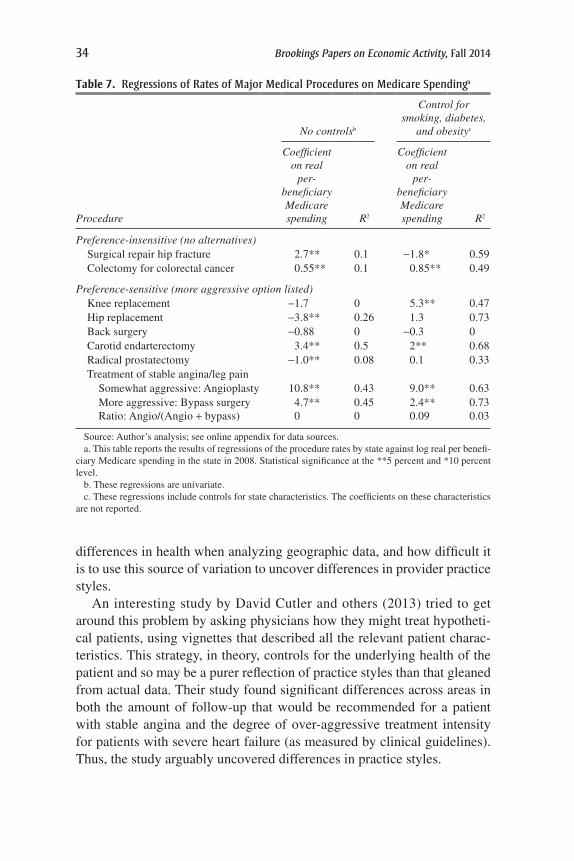
Table 7 shows the relationship between Medicare expenditures and the procedures described by Dartmouth as (i) having no alternatives and (ii) being preference-sensitive. The first column reports the results of bivar-iate regressions of procedure rates (or for bypass surgery and angioplasty, the ratio of the two) on real Medicare spending per beneficiary. The second column shows the results when health attributes—diabetes, smoking, and obesity—are controlled for.
The table suggests a number of conclusions. First, high-spending states are more likely than low-spending states to undertake procedures for which there are no alternatives, showing that underlying health rates differ. Sec-ond, comparing the R2 from the first and second set of regressions shows that simple measures of differences in underlying health can explain a sig-nificant fraction of the differences in procedure use. Third, the variation in usage of different procedures may reflect differences in the appropriateness of such procedures across areas, rather than differences in practice styles.
Indeed, without adjustment for underlying health, low-spending states appear to be more likely to provide some forms of aggressive care, namely hip replacement and radical prostatectomy. For other elective and arguably aggressively interventionist procedures, including knee replacement and back surgery, there appears to be no systematic relationship between aver-age Medicare spending and usage rates. Finally, while high-spending states are much more likely to have higher rates of cardiac procedures, even when smoking, diabetes, and obesity rates are taken into account, the share of such interventions that are more aggressive is unrelated to average spend-ing levels. These results show how important it is to control for underlying

Louise sheiner 33
AL
AR
AZ
CA
CO
CT
DE
FL
GA
IA
ID
IL
IN
KS
KYLA
MA
MD
ME
MIMN
MO
MS
MT
NC
ND
NE
NHNJ
NM
NV
NY
OH
OK
ORPA
RI
SC
SD
TN
TX
UT
VA
VTWA
WI
WV
WY
6.0
6.5
7.0
7.5
8.0
8.5
0.06 0.08 0.10Share diabetic
Rate of hip fracture repair
Rate of hip replacement
3
4
5
ALAR
AZ
CA
CO
CTDE
FL
GA
IA
ID
ILINKS
KY
LA
MAMD
ME MI
MN
MO
MS
MT
NC
ND
NE
NH
NJNM
NVNY
OH
OK
OR
PARI
SC
SD
TN
TX
UT
VA
VTWA
WI
WV
WY
0.06 0.08 0.10Share diabetic
Source: Author’s analysis; see online appendix for data sources.
Figure 6. hip Fracture repair and hip replacement rates: Correlations with Diabetes rates, by state
34 Brookings Papers on Economic Activity, Fall 2014
differences in health when analyzing geographic data, and how difficult it is to use this source of variation to uncover differences in provider practice styles.
An interesting study by David Cutler and others (2013) tried to get around this problem by asking physicians how they might treat hypotheti-cal patients, using vignettes that described all the relevant patient charac-teristics. This strategy, in theory, controls for the underlying health of the patient and so may be a purer reflection of practice styles than that gleaned from actual data. Their study found significant differences across areas in both the amount of follow-up that would be recommended for a patient with stable angina and the degree of over-aggressive treatment intensity for patients with severe heart failure (as measured by clinical guidelines). Thus, the study arguably uncovered differences in practice styles.
table 7. regressions of rates of Major Medical Procedures on Medicare spendinga
No controlsb
Control for smoking, diabetes,
and obesityc
Procedure
Coefficient on real
per- beneficiary Medicare spending R2
Coefficient on real
per- beneficiary Medicare spending R2
Preference-insensitive (no alternatives) Surgical repair hip fracture 2.7** 0.1 -1.8* 0.59 Colectomy for colorectal cancer 0.55** 0.1 0.85** 0.49
Preference-sensitive (more aggressive option listed) Knee replacement -1.7 0 5.3** 0.47 Hip replacement -3.8** 0.26 1.3 0.73 Back surgery -0.88 0 -0.3 0 Carotid endarterectomy 3.4** 0.5 2** 0.68 Radical prostatectomy -1.0** 0.08 0.1 0.33 Treatment of stable angina/leg pain Somewhat aggressive: Angioplasty 10.8** 0.43 9.0** 0.63 More aggressive: Bypass surgery 4.7** 0.45 2.4** 0.73 Ratio: Angio/(Angio + bypass) 0 0 0.09 0.03
Source: Author’s analysis; see online appendix for data sources.a. This table reports the results of regressions of the procedure rates by state against log real per benefi-
ciary Medicare spending in the state in 2008. Statistical significance at the **5 percent and *10 percent level.
b. These regressions are univariate.c. These regressions include controls for state characteristics. The coefficients on these characteristics
are not reported.
Louise sheiner 35
Nevertheless, a key question remains, whether those differences in practice styles are correlated with other factors that affect spending. Prac-tice styles, as noted earlier, might reflect the health of the typical patient.25 Furthermore, if better practice styles are associated with higher social capi-tal, as had been hypothesized, then any regression of spending on practice styles will pick up both the effects of physician decision making as well as the underlying health differences that contribute to differences in spend-ing. Thus, the finding by Cutler and others that these differences in practice styles can explain up to 36 percent of end-of-life spending and 17 percent of overall Medicare spending may reflect the fact that places where pro-viders are likely to practice efficient medicine are also those places where patients are in generally good health. So long as the differences in practice styles are not random, the vignette approach alone can’t solve the basic dif-ficulty of disentangling the sources of spending variation.
IV.D. Clues from the non-Medicare Population
If the geographic variation in Medicare spending is reflective of prac-tice styles, then one might expect to see a similar variation in spending, holding all else equal, for non-Medicare patients. Similarly, if some areas have poorer health than others, one might expect to see higher spending in places with poor health as well. To test these hypotheses, I use two differ-ent measures of non-Medicare health expenditures. The first method aims to capture all acute health spending received by non-Medicare beneficia-ries. To do this, I calculate Medicare spending by service (hospital, physi-cian, and other professional) and “gross it up” to reflect total expenditures on behalf of Medicare beneficiaries, including deductibles and coinsur-ance.26 I then take total expenditures on hospitals, physicians, and other
25. The “mean health” explanation can’t directly explain the variation in the aggres-siveness of care recommended for the heart failure patients—after all, such interventions would have been even more inappropriate for patients in worse health. However, research-ers (McGlynn and others 1994) have found that in areas where physicians perform a greater volume of inappropriate treatments, they also perform a greater volume of appropriate care, suggesting that the mean health in an area might still explain the degree of aggressive intervention. A vignette in which the hypothetical patient actually warranted aggressive intervention could shed light on this question.
26. I used the average Medicare share of payments for physician and hospital services from the Medicare Beneficiary Survey to calibrate the out-of-pocket spending by service; in particular, I assumed that Medicare covered 86 percent of hospital expenses and 69 per-cent of physician and other professional expenses; an alternative measure that assumed that Medicare covered a greater share of expenditures—93 percent for hospitals and 85 percent for physicians—yielded very similar results.
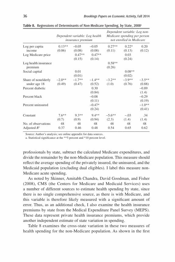
36 Brookings Papers on Economic Activity, Fall 2014
professionals by state, subtract the calculated Medicare expenditures, and divide the remainder by the non-Medicare population. This measure should reflect the average spending of the privately insured, the uninsured, and the Medicaid population (excluding dual eligibles). I label this measure non-Medicare acute spending.
As noted by Skinner, Amitabh Chandra, David Goodman, and Fisher (2008), CMS (the Centers for Medicare and Medicaid Services) uses a number of different sources to estimate health spending by state, since there is no single comprehensive source, as there is with Medicare, and this variable is therefore likely measured with a significant amount of error. Thus, as an additional check, I also examine the health insurance premiums by state from the Medical Expenditure Panel Survey (MEPS). These data represent private health insurance premiums, which provide another independent estimate of state variation in spending.
Table 8 examines the cross-state variation in these two measures of health spending for the non-Medicare population. As shown in the first
table 8. regressions of Determinants of non-Medicare spending, by state, 2008a
Dependent variable: Log health insurance premium
Dependent variable: Log non-Medicare spending per person
not enrolled in Medicare
Log per capita income
0.13**(0.06)
-0.05(0.08)
-0.05(0.08)
0.27**(0.11)
0.22*(0.13)
0.20(0.12)
Log Medicare price 0.47**(0.15)
0.47**(0.14)
0.03(0.24)
Log health insurance premium
0.58**(0.26)
Social capital 0.01(0.01)
0.08**(0.02)
Share of nonelderly under age 18
-2.0**(0.49)
-1.7**(0.47)
-1.4**(0.52)
-3.2**(1.0)
-3.9**(0.76)
-3.5**(0.88)
Percent diabetic 0.30(0.84)
-0.89(1.4)
Percent black -0.08(0.11)
-0.29(0.19)
Percent uninsured -0.47*(0.24)
-1.0**(0.41)
Constant 7.6**(0.7)
9.3**(0.9)
9.4**(0.94)
-5.6**(2.3)
-.03(1.4)
.34(1.4)
No. of observations 48 48 48 48 48 48Adjusted R2 0.37 0.46 0.48 0.54 0.65 0.62
Source: Author’s analysis; see online appendix for data sources.a. Statistical significance at the **5 percent and *10 percent level.

Louise sheiner 37
column, the share of young people and per capita income can account for some of the variation in health insurance premiums across states. Adding in the log of the Medicare price (which is partly based on hospital wage rates) increases the fit. Social capital has no predictive value for health insurance premiums; similarly, the rate of diabetes in the population has no significant effect on premiums, although the rate of uninsurance appears to be loosely (and negatively) associated with private insurance premiums.
The second set of columns in table 8 examines the determinants of non-Medicare spending more broadly. Spending is higher where per capita income is higher and where the share of kids is lower. Furthermore, there is a significant relationship between non-Medicare health spending and the MEPS health insurance premium, with each 1-percent increase in the premium associated with a 0.6-percent increase in average non-Medicare spending. This finding suggests that the measure of non-Medicare health spending is a reasonable one.
Social capital is a significant predictor of non-Medicare spending, but the relationship is opposite to that for Medicare spending: Higher levels of social capital are associated with lower Medicare spending, but higher non-Medicare spending. The final column of table 8 shows that the relationship between social capital and non-Medicare spending is largely accounted for by the relationship between social capital and insurance rates. States with low social capital have high rates of uninsurance and consequently low levels of spending. (These states might also have low reimbursement rates, which would also contribute to lower overall spending.) As with the private health insurance premium regressions, the rate of diabetes does not predict health spending, and other health factors, including obesity rates, smoking rates, and overall health status (not shown) were found to be insignificant as well.
The lack of a relationship between non-Medicare spending and popula-tion health is likely due to a combination of factors, including the fact that less of the health spending of the nonelderly is related to underlying poor health (and more of it is related to childbirth, preventive care, accidents, and random health shocks), those in poor health are less likely to have insurance, and the effects of poor health on spending probably cumulate over time and have much less of an impact on health spending at younger ages. In addition, some of the variation in spending across states reflects price variation (likely reflecting the competitiveness of the health provider and insurance markets), which would not be affected by health status (Institute of Medicine 2013).
Table 9 examines the relationship between health spending for the non-elderly population and Medicare spending. The first three columns of the table explore the relationship between private health insurance premiums
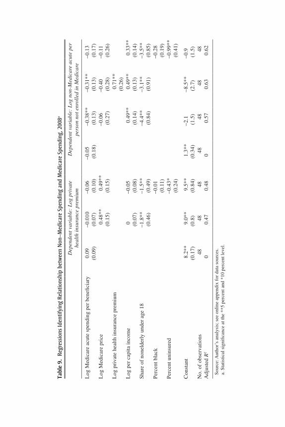
tabl
e 9.
reg
ress
ions
iden
tifyi
ng r
elat
ions
hip
betw
een
non
–Med
icar
e sp
endi
ng a
nd M
edic
are
spen
ding
, 200
8a
Dep
ende
nt v
aria
ble:
Log
pri
vate
he
alth
insu
ranc
e pr
emiu
mD
epen
dent
var
iabl
e: L
og n
on-M
edic
are
acut
e pe
r pe
rson
not
enr
olle
d in
Med
icar
e
Log
Med
icar
e ac
ute
spen
ding
per
ben
efici
ary
0.09
(0.0
9)-0
.010
(0.0
7)-0
.06
(0.1
0)-0
.05
(0.1
8)-0
.38*
*(0
.13)
-0.3
1**
(0.1
3)-0
.13
(0.1
7)L
og M
edic
are
pric
e0.
48**
(0.1
5)0.
49**
(0.1
5)-0
.06
(0.2
7)-0
.40
(0.2
8)-0
.11
(0.2
6)L
og p
riva
te h
ealt
h in
sura
nce
prem
ium
0.71
**(0
.26)
Log
per
cap
ita
inco
me
0 (0.0
7)-0
.05
(0.0
8)0.
49**
(0.1
4)0.
49**
(0.1
3)0.
33**
(0.1
4)S
hare
of
none
lder
ly u
nder
age
18
-1.8
**(0
.46)
-1.5
**(0
.49)
-4.4
**(0
.84)
-3.1
**(0
.91)
-3.5
**(0
.85)
Per
cent
bla
ck-0
.01
(0.1
1)-0
.28
(0.1
9)P
erce
nt u
nins
ured
-0.4
3*(0
.24)
-0.9
9**
(0.4
1)
Con
stan
t8.
2**
(0.1
7)9.
0**
(0.8
)9.
5**
(0.8
4)1.
3**
(0.3
4)-2
.1(1
.5)
-8.5
**(2
.7)
-0.9
(1.5
)N
o. o
f ob
serv
atio
ns48
4848
4848
4848
Adj
uste
d R
20
0.47
0.48
00.
570.
630.
62
Sour
ce: A
utho
r’s
anal
ysis
; see
onl
ine
appe
ndix
for
dat
a so
urce
s.a.
Sta
tistic
al s
igni
fican
ce a
t the
**5
per
cent
and
*10
per
cent
leve
l.

Louise sheiner 39
and acute Medicare spending per beneficiary; they show that there is virtu-ally no relationship. In contrast, once per capita income and the share of young people (under age 18) is taken into account, non-Medicare spend-ing (shown on the right side of the table) appears to be negatively related to Medicare spending, with every 1-percent increase in Medicare spend-ing associated with a 0.4-percent decrease in non-Medicare spending. This negative relationship appears to reflect the opposing associations between social capital and Medicare and non-Medicare spending: Once the black percentage of the population and the share that is uninsured are taken into account (the final column), the negative relationship becomes much smaller and insignificant.
These regressions show that there is little relationship between private health spending and Medicare. Michael Chernew and others (2010) obtain similar results when comparing Medicare spending to spending for those insured through large employers: although in-patient hospital utilization was similar for Medicare and non-Medicare beneficiaries, total spending was not.
But Medicare and total non-Medicare spending appear to be negatively correlated, and factors that increase Medicare spending—such as health variables, percent black, and percent uninsured—either have no effect on non-Medicare spending (health variables) or reduce it (percent black and percent uninsured). Thus, places with poor health, high rates of uninsurance, and a large black population—like Mississippi and Louisiana—have high Medicare spending and low non-Medicare spending. Conversely, places with the opposite characteristics—like Vermont and Minnesota—have rela-tively high non-Medicare spending and low Medicare spending. This find-ing suggests that some form of “volume shifting” is likely occurring. Places where health care resources for the non-Medicare population are low may rely on Medicare to help finance their health care systems, whereas places where private resources are more ample may have less need to do so.27
V. the relationships between spending, Physician Workforce composition, and Quality
In general, Medicare and non-Medicare beneficiaries use the same providers—the same hospitals and the same physicians—so decisions made by these providers are likely to reflect the policies and payment
27. Evaluating the efficiency effects of such volume shifting is difficult, because Medi-care reimbursements are unlikely to reflect the marginal cost of procedures, particularly for providers, like hospitals, that have high fixed costs.

40 Brookings Papers on Economic Activity, Fall 2014
generosity of all the payers. Thus, a complete analysis of the determinants of health-system-wide characteristics, like physician workforce composi-tion and quality, needs to take into account spending by both Medicare and non-Medicare beneficiaries, as well as the demographic characteristics of different areas.
V.A. Medicare Spending and the Physician Workforce
Baicker and Chandra (2004) showed that states with a greater share of physicians who are general practitioners have significantly lower Medicare spending and significantly higher quality than states with a higher share of specialists. This is an interesting finding because it suggests an actual policy that one might follow to lower costs and improve quality. One con-sideration, however, is that the mix of physicians is likely to depend on the entire population’s demand for services. If the elderly use specialists at a different rate than the nonelderly, the mix of spending by the nonelderly and the elderly might affect the composition of the physician workforce. More generally, the strong dependence of Medicare spending on health and demographic variables suggests that studies that do not control for these factors could be misleading. Richard Cooper (2009a) argues that the share of general practitioners is a marker for sociodemographic differences, but does not test the implications of controlling for these characteristics.
Table 10 suggests that the relationship between spending and the com-position of the physician workforce is not as clear as suggested by Baicker
table 10. regressions identifying relationships between Physician workforce Characteristics and spendinga
Dependent variable: Log spending per beneficiary, 2008
Medicare Non-Medicare
General practitioners per 1,000 -0.49** -0.04 0.51** 0.33*Total physicians per 1,000 0.05* 0.04* 0.06* 0.03Log per capita income 0.13 0.38** 0.34** 0.29**Log Medicare price -0.14 0.34Percent diabetic 4.6**Percent black 0.23 -0.16Percent uninsured 0.37 -0.8*Share of nonelderly under age 18 -1.7 -2.1*
Constant 0.59 -2.7** -2.3* -1.4No. of observations 48 48 48 48Adjusted R2 0.43 0.74 0.63 0.65
Source: Author’s analysis; see online appendix for data sources.a. Statistical significance at the **5 percent and *10 percent level.

Louise sheiner 41
and Chandra. The first column of the table reports the results from a regres-sion of per-beneficiary acute Medicare spending on physician composition, mean state income, and Medicare prices, similar to the regression run by Baicker and Chandra. Holding the number of physicians constant, there is a strong negative relationship between the number of general/family prac-titioners per 1,000 population and the level of Medicare spending—which matches the Baicker and Chandra result. However, once the rate of diabe-tes, the rate of uninsured, and the black percentage of the population are included in the regression, the relationship disappears.
The right-most pair of columns reports the results when the dependent variable is non-Medicare spending. Here, the story is the opposite: the more general/family practitioners there are, the higher non-Medicare spending is. Even when one includes the share of the population that is black and the share uninsured in the regression, this effect persists. Finally, there is no relationship between health insurance premiums and physician workforce characteristics. These results suggest that the share of general practitioners does appear to be a marker for population characteristics, as Cooper sug-gests, and once this is taken into account there appears to be no system-atic relationship between these broad workforce characteristics and health spending.
V.B. Medicare Spending and Quality
Much of the Dartmouth group’s work has argued that geographic areas where health spending is higher do not show any better health outcomes than those where it is lower, suggesting that there is no payoff for that extra spending. But some earlier research, including that by Katherine Baicker and Chandra (2004) and Skinner, Douglas Staiger, and Fisher (2006), argues that higher spending is actually associated with lower quality, per-haps because high-spending areas are less likely to adopt cost-saving and quality-improving technologies. In contrast, when Cooper (2009b) exam-ines total spending by state (note that this measure is highly correlated with non-Medicare spending), he concludes that more spending is associated instead with higher quality.
The quality measure used in these studies—the Jencks index—is a ranking of states based upon how well they comply with recommended medical guidelines. For example, the index includes measures of whether hospitals treat heart attack victims with beta blockers, whether patients get antibiotics during the recommended 24 hours before surgery, and whether ACE inhibitors are appropriately prescribed for patients with heart failure.

42 Brookings Papers on Economic Activity, Fall 2014
One advantage of this index is that, unlike outcomes-based measures of quality, it does not need to be adjusted for differing health risks, because it is based on standards of care that virtually all patients should receive. A disadvantage, however, is that because it is measuring relatively simple and agreed-upon processes of care, it may be biased toward finding a negative relationship between spending and quality. As demonstrated by Chandra and Staiger (2007) with respect to heart attack treatment, geo-graphic areas differ in the type of care they specialize in: areas where heart attack victims tend to be treated surgically are worse at medi-cal management, and vice versa. Thus, for patients who need surgery, intensive-treatment areas are best, and for patients who do not require surgery, less intensive areas are better. However, because the Jencks index only includes measures of medical management (five of the twenty-three measures in the index relate to timeliness and appropriateness of aspi-rin, beta blockers, and ACE inhibitors for heart attack victims), it will be biased toward showing higher quality for areas that practice less intensive forms of medicine.
Furthermore, the Jencks index also includes measures that likely depend on demographic and socioeconomic characteristics. For example, it includes measures of whether the population (not just Medicare beneficiaries) gets flu shots, whether women have mammograms, and whether diabetics get appropriate screening tests (biennial eye exams, lipid profiles, and blood sugar tests). In practice, whether individuals receive these types of services may depend on whether there are clinics nearby, whether they have easy access to transportation, whether they have the time or the ability to take time off work for an appointment, whether they have insurance, and so on—and these are all likely related to demographic characteristics.
How sensitive are the literature’s conclusions on quality and spending to the inclusion of health and insurance controls? The first column of table 11 reproduces the result found in much of the literature: Medicare spending is higher in areas with low quality, according to the Jencks ranking. However, similar to the findings for physician workforce composition, health spend-ing for the non-Medicare population (second row) has the opposite rela-tionship to quality, with more spending associated with higher quality. This surprising finding is evident in figure 7, which plots Medicare and non-Medicare spending against the Jencks ranking. Turning back to Table 11, the second column shows that there is also a positive, but insignificant, relationship between private health insurance premiums and quality. How-ever, as shown in columns 3 and 4, the relationships between quality and

table 11. regressions identifying relationships between health spending and Jencks index of Qualitya
Dependent variable: Jencks quality ranking, 2000
Log price-adjusted Medicare spending per beneficiary
-80**(14)
-88**(15)
-17(17)
-14(17)
Log non-Medicare spending per person not enrolled in Medicare
39**(12)
5(12)
Log health insurance premium 40(25)
17(20)
Share of nonelderly under age 18 -170**(83)
-164**(76)
Log per capita income 12(12)
24*(12)
-25**(11)
-26**(11)
Percent diabetic -652**(138)
-683**(138)
Percent uninsured -128**(35)
-127**(34)
Constant -49(118)
-451**(197)
378**(115)
260(185)
No. of observations 48 48 48 48Adjusted R2 0.59 0.52 0.78 0.78
Source: Author’s analysis; see online appendix for data sources; Jencks quality ranking is for 2000; all other data are for 2008.
a. Statistical significance at the **5 percent and *10 percent level.
AL
AR
AZ
CA
COCT
DE
FL
GA
IA
ID
IL
IN
KS
KY
LA
MA
MD
ME
MI
MN
MO
MS
MT
NC
ND
NE
NH
NJ
NM NV
NY
OH
OK
OR
PA
RI
SC
SD
TN
TX
UT
VA
VT
WA
WI
WV
WY
AL
AR
AZ
CA
CO CT
DE
FLGA
IA
ID
IL
IN
KS
KY
LA
MA
MD
ME
MI
MN
MO
MS
MT
NC
ND
NE
NH
NJ
NMNV
NY
OH
OK
OR
PA
RI
SC
SD
TN
TX
UT
VA
VT
WA
WI
WV
WY
10
20
30
40
50
3,000 4,000 5,000 6,000 7,000 8,000
Jencks quality ranking
Price-adjusted Medicare spending Non-Medicare spendingHealth spending
Source: Author’s analysis; see online appendix for data sources.
Figure 7. Quality ranking and health spending, by state

44 Brookings Papers on Economic Activity, Fall 2014
health spending are not robust, and they are eliminated by simply control-ling for overall health and access to care.
Table 12 examines the Baicker and Chandra (2004) finding that more generalists leads to higher quality. Here, too, including the share of the population that is uninsured, the share that is black, and the share that is under age 18 leads one to conclude that there is little relationship between the variation in physician composition across states and the variation in quality.
The point of these exercises is not to argue that there is no relationship between physician workforce composition and spending or between quality and Medicare spending, but that such relationships are very hard to tease out from cross-state differences in Medicare spending. As noted previ-ously, states with high levels of Medicare spending are very different from states with low levels of Medicare spending, and they are different in ways that are likely to affect all dimensions of the health system. While includ-ing controls for these differences is helpful and important, it is sometimes difficult to know whether the controls are exogenous or endogenous. For example, it could be that Medicare spending is high in places with a large black population because such populations have a lower share of general
table 12. regressions of effects of Physician Composition on Quality ranking
Dependent variable: Jencks quality ranking, 2000
(1) (2) (3)
General practitioners per 1,000 63**(14)
22**(11)
4.6(13)
Total physicians per 1,000 9.5**(2.6)
0.7(2.1)
-4.1(3.1)
Percent diabetic -592**(0.87)
-683**(95)
Percent uninsured -132**(39)
-131**(37)
Share of nonelderly under age 18 -227**(109)
Constant -85**(12)
29**(16)
123**(47)
No. of observations 48 48 48Adjusted R2 0.34 0.73 0.75
Source: Author’s analysis; see online appendix for data sources; Jencks quality ranking is for 2000; all other data are for 2008.
a. Statistical significance at the **5 percent and *10 percent level.

Louise sheiner 45
practitioners, or it could be that Medicare spending is high in places with a lower share of general practitioners because such places have a large black population with high Medicare expenses. The finding that the relationships between non-Medicare spending, quality, and physician composition are opposite to those of Medicare spending suggest that important interactions are occurring that are difficult to control for.
A recent Institute of Medicine report also examines the relationship between health utilization and quality, using a variety of new metrics that have been introduced in recent years. The report concentrates on three composite measures of quality: (i) a measure that examines patient safety (absence of errors) in hospitals; (ii) a measure that examines mortality rates; and (iii) a measure that examines avoidable hospital admissions28 (Institute of Medicine 2013, p. 16). It finds that “areas with high scores on some quality measures do not necessarily have high scores on others,” suggesting that areas cannot be classified by their “quality.” These findings reinforce the view that any geographic-level correlations between spending and overall quality are unlikely to be causal.
VI. Growth rates
Finally, it is important to consider the implications of these findings for analyzing the growth of Medicare spending across states. The Dartmouth group’s methodology often examines changes in the level of Medicare spending over time—thus, for example, Skinner, Staiger, and Fisher (2006) compare dollar changes in Medicare spending with changes in heart-attack survival rates to argue that increased spending was negatively related to increased survival. Similarly, Baicker and Chandra (2004) find that increases in the level of Medicare spending are associated with reductions in quality.
This methodology would make sense if the prices paid by Medicare and the health needs of the populations did not vary across states. But, to the extent that the variation in the level of spending is associated with state attributes, a better approach is to compare the growth rates of spending across states.29 Otherwise, high-spending states with the same growth rate as low-spending states will appear to have increased
28. Unfortunately, only a subset of these measures is available to the public.29. Even by the Dartmouth researchers’ calculations, 30 percent of the variation in medi-
cal spending derives from differences in income and health across areas.

46 Brookings Papers on Economic Activity, Fall 2014
spending more, thus making it more likely that increased spending will be found to be not worthwhile.30
Furthermore, part of the message from the Dartmouth researchers is that low-cost areas are also areas that are more likely to adopt cost-effective technologies and less likely to adopt expensive technologies that do not increase quality. So, are low-spending states also low-growth states?
Figure 8 examines changes in relative Medicare spending over time (between 1991 and 2008). As shown in the top panel, the ranking of state Medicare spending has been fairly stable. However, as shown in the bot-tom panel, there is a strong negative correlation between health spending growth and initial level of health spending. Low-spending states tend to increase spending at a faster pace than high-spending states. For exam-ple, Medicare spending rose at an average rate of 6.2 percent per year in Nebraska but at only 3.7 percent per year in Pennsylvania.
Table 13 reports the results from a simple regression of health spend-ing growth on the initial spending level (growth in per capita income and insurance were not significant and are not included). The negative cor-relation between the level of health spending and the subsequent growth is observed from 1991 to 2000 and from 2000 to 2008. Thus, the data do not support the idea that low-spending states are low-growth states that adopt technology in a more cost-effective manner, and understanding regional variation is unlikely to be the key to figuring out how to bend the cost curve.31
30. More formally, if Medicare spending per beneficiary, M, is equal to spending per condition, C, times conditions per beneficiary (a function of health), H, then Medicare spend-ing in state i in year 1 is just M1
i = C1iHi and spending in year 2 is M2
i = C2iHi. Then, the change
in Medicare spending is M2i - M1
i = Hi(C2i - C1
i) and locations with greater health needs will have greater change in spending for any given increase in cost per case. Of course, taking logs yields log(M1
i) = log(C1i) + log(Hi) and thus change in the logs (that is, percent change)
will yield a measure that is unaffected by state health.31. Fisher, Bynum, and Skinner (2009) write in the New England Journal of Medicine:
“To slow spending growth, we need policies that encourage high-growth (or high-cost) regions to behave more like low-growth, low-cost regions—and that encourage low-cost, slow-growth regions to sustain their current trends.” However, their view that there are “low-cost, slow-growth” (p. 851) regions comes from looking at the relationship between growth rates and end-of-period spending, rather than the more appropriate beginning-of-period mea-sure (because places where spending grows more slowly will more likely have lower end-of-period spending).

Louise sheiner 47
Log acute Medicare spending per beneficiary, 2008
Log acute Medicare spending per beneficiary, 1991
ALAR
AZ
CA
CO
CT DE
FL
GA
IA
ID
IL
INKS
KY
LAMA
MD
ME
MI
MN
MO
MS
MT
NC
ND
NE
NH
NJ
NM
NV
NY
OH
OK
OR
PA
RI
SC
SD
TN
TX
UT
VAVT WA
WIWV
WY
8.6
8.7
8.8
8.9
9
9.1
7.6 7.8 8 8.2
Log acute Medicare spending per beneficiary, 1991
ALAR
AZ
CACO
CT
DE
FL
GA
IAID
IL
IN
KS
KY
LAMA
MDME MI
MN
MO
MS
MT
NCND
NE
NHNJ
NM NV
NYOHOKOR
PA
RI
SC
SD
TN
TX
UT
VA
VT
WA
WI
WVWY
0.04
0.045
0.05
0.055
0.06
7.8 8 8.2
Growth rate, 1991–2008
Source: Author’s analysis; see online appendix for data sources.
Figure 8. Medicare spending growth, 1991–2008

48 Brookings Papers on Economic Activity, Fall 2014
VII. conclusions
The evidence presented in this paper shows that most of the variation in Medicare spending across states is associated with factors that affect health and health behaviors, rather than with random variation in practice styles. Isolating the exact channels through which differences in health affect Medicare spending is difficult, however, because both the need for health spending and provider practice styles will likely be affected by variations in population health and the variables that are correlated with it.
The paper has several findings that suggest that the variation in Medi-care spending does not represent wasteful spending that could be easily eliminated without significant effects on the health system. First, popu-lation characteristics have more explanatory power for Medicare spend-ing than measures of social capital, indicating that the variation in patient characteristics is more important than variation in provider characteristics. Second, health measures are significantly more correlated at the state level than at the individual level, making it likely that state-level regressions do
table 13. growth rates and Persistence in Medicare spending
Persistence of spending
Regression of log per beneficiary acute Medicare spending on its lag
Dependent variable year Lag year
Coefficient on lagged Medicare
spending R2
No. of observations
(1) 2008 2000 0.87** 0.91 48(2) 2000 1991 0.78** 0.76 48(3) 2008 1991 0.71** 0.75 48
Relationship between persistence and growth rate
Regression of growth rate of acute Medicare spending on the lagged log of acute per beneficiary medical spending
Growth rate years
Lag spending year
Coefficient on lagged Medicare
spending R2
No. of observations
(1) 2000–2008 2000 -0.02** 0.16 48(2) 1991–2000 1991 -0.03** 0.18 48(3) 1991–2008 1991 -0.02** 0.32 48
Source: Author’s analysis; see online appendix for data sources.a. Statistical significance at the **5 percent level.

Louise sheiner 49
a better job of controlling for unobserved variation in population health.32 Third, there does not seem to be a significant relationship between the use of “preference-sensitive procedures” and the level of Medicare spending. Fourth, states with high levels of Medicare spending tend to have lower levels of non-Medicare spending. Providers in these last states might face greater financial difficulties than providers elsewhere and may volume-shift to Medicare patients in order to cover costs.
The paper also shows that conclusions about the relationships between health spending, physician composition, and quality are sensitive to the inclusion of variables like the share of the population that is uninsured, black, or diabetic. What this sensitivity demonstrates is the difficulty of using the geographic variation in spending for hypothesis testing. It is not surprising that states in the South spend more on Medicare and have worse outcomes. These states perform significantly worse in numerous areas, including high school graduation rates, test scores, and teenage pregnancy.33 There are many ways that such differences can affect health utilization and outcomes, including differences in underlying health, social supports and social stressors, patient self-care and advocacy, ease of access to services, capabilities of hospital and physician nurses and technicians, and cultural differences in attitudes toward care. A comparison of health spending in Mississippi with health spending in Minnesota is not likely to pro-vide a useful metric of the “inefficiencies” of the health system in isolation; rather, the difference in spending likely mirrors broader societal prob-lems unrelated to the health system per se. This finding suggests that reduc-ing the geographic variation in health spending will not be an easy task.34
Finally, the evidence also suggests that low-cost states are not low-growth states. Thus, the geographic variation in Medicare spending is probably not the key to finding ways to slow spending growth while continuing to improve quality over time.
32. Indeed, the results from these state-level regressions are quite consistent with those found by Finkelstein and others (2014) using detailed data on movers. They find that 40 to 50 percent of the variation in price-adjusted spending is attributable to variation in individual health; my regressions suggest that adding health and demographic measures improves the fit by about 60 percent. The difference from the state-level regressions suggests that volume shifting and practice styles geared toward mean health also have explanatory power.
33. For teen pregnancy rates, see http://thenationalcampaign.org/data/compare/1701; for test scores, see http://www.act.org/newsroom/data/2014/states.html; for high-school gradua-tion rates, see http://nces.ed.gov/pubs2011/dropout08/figures/figure_06.asp.
34. Further, the differences among states also suggest that the strategies to improve health and lower spending might need to be targeted to the specific characteristics of the states.

50 Brookings Papers on Economic Activity, Fall 2014
AcknoWLeDGMents I would like to thank Greg Duffee, Glenn Follette, Byron Lutz, Vasia Panousi, David Wessel, the editors, my discussants David Cutler and Douglas Staiger, and the participants at the Federal Reserve System Regional Conference, the Johns Hopkins microeconomics seminar, the Brookings Institution seminar, and the NBER Health Conference for very helpful comments. I am grateful to Brendan Mochoruk for excellent research assistance.
references
ACT, Inc. “2014 ACT National and State Scores.” (http://www.act.org/newsroom/data/2014/states.html)
Baicker, Katherine, and Amitabh Chandra. 2004. “Medicare Spending, the Physi-cian Workforce, and Beneficiaries’ Quality of Care.” Health Affairs W4-194, 7 (April).
Chandra, Amitabh, and Douglas Staiger. 2007. “Productivity Spillovers in Health Care: Evidence from the Treatment of Heart Attacks.” Journal of Political Economy 115, no. 1: 103–40.
Chernew, Michael E., Lindsay M. Sabik, Amitabh Chandra, Teresa B. Gibson, and Joseph P. Newhouse. 2010. “Geographic Correlation between Large-Firm Commercial Spending and Medicare Spending.” American Journal of Managed Care 16, no. 2: 131–38.
Clemens, Jeffrey, and Joshua Gottlieb. 2012. “Do Physicians’ Financial Incentives Affect Medical Treatment and Patient Health.” Stanford University (SIEPR). (http://siepr.standford.edu/publicationsprofile/2447)
CMS Geographic Variation Public Use Files. (https://www.cms.gov/Research- Statistics-Data-and-Systems/Statistics-Trends-and-Reports/Medicare-Geographic- Variation/GV_PUF.html)
Cooper, Richard. 2009a. “States with More Physicians Have Better-Quality Health Care.” Health Affairs 28, no. 1: w91–102.
———. 2009b. “States with More Health Care Spending Have Better-Quality Health Care: Lessons about Medicare.” Health Affairs 28, no. 1: w103–115.
Cutler, David M., and Louise Sheiner. 1999. “The Geography of Medicare.” American Economic Review 89, no. 2: pp. 228–33, May.
Cutler, David, Jonathan Skinner, Ariel Dora Stern, and David Wennberg. 2013. “Physician Beliefs and Patient Preferences: A New Look at Regional Varia-tion in Health Care Spending.” Working Paper no. 19320. Cambridge, Mass.: National Bureau of Economic Research.
Dartmouth Atlas Project. 2007. “Preference-Sensitive Care.” Topic Brief. The Dartmouth Institute for Health Policy and Clinical Practice. (http://www.dart mouthatlas.org/downloads/reports/preference_sensitive.pdf)
Doyle, Joseph. 2007. “Returns to Local-Area Health Care Spending: Using Health Shocks to Patients Far from Home.” Working Paper no. 13301. Cambridge, Mass.: National Bureau of Economic Research.

Louise sheiner 51
Finkelstein, Amy, Matthew Gentzkow, and Heidi Williams. 2014. “Sources of Geo-graphic Variation in Health Care: Evidence from Patient Migration.” Working Paper no. 20789. Cambridge, Mass.: National Bureau of Economic Research.
Finkelstein, Amy, Sarah Taubman, Bill Wright, Mira Bernstein, Jonathan Gruber, Joseph Newhouse, Heidi Allen, Katherine Baicker, and the Oregon Health Study Group. 2011. “The Oregon Health Insurance Experiment: Evidence from the First Year.” Quarterly Journal of Economics 127, no. 3: 1057–1106.
Fisher, Elliott, Julie Bynum, and Jonathan Skinner. 2009. “Slowing the Growth of Health Care Costs—Lessons from Regional Variation.” New England Journal of Medicine 360: 849–52.
Fisher, Elliott, David E. Wennberg, Thérèsa A. Stukel, Daniel J. Gottlieb, F. L. Lucas, and Étoile L. Pinder. 2003. “The Implications of Regional Variations in Medicare Spending—Part 1: The Content, Quality, and Accessibility of Care.” Annals of Internal Medicine 138, no. 4: 273–87: 273.
Gawande, Atul. 2009. “The Cost Conundrum: What a Texas Town Can Teach Us About Healthcare.” New Yorker, June.
Glaeser, Edward, David Laibson, Jose Scheinkman, and Christine Soutter. 1999. “What is Social Capital? The Determinants of Trust and Trustworthiness.” Working Paper no. 7216. Cambridge, Mass.: National Bureau of Economic Research.
Hadley, Jack, and James Reschovsky. 2006. “Medicare Fees and Physicians’ Medicare Service Volume: Beneficiaries Treated and Services per Benefi-ciary.” International Journal of Health Care Finance Economics 6, no. 2: 131–50.
Institute of Medicine. 2013. “Variation in Health Care Spending: Target Deci-sion Making, Not Geography.” Washington: National Academies Press.
Jacobson, Mireille, A. James O’Malley, Craig C. Earle, Juliana Pakes, Peter Gaccione, and Joseph P. Newhouse. 2006. “Does Reimbursement Influence Che-motherapy Treatment for Cancer Patients?” Health Affairs 25, no. 2: 437–43.
Janghorbani, Mohsen, Diane Feskanich, Walter C. Willett, and Frank Hu. 2006. “Prospective Study of Diabetes and Risk of Hip Fracture: The Nurses’ Health Study.” Diabetes Care, July.
Jencks, Stephen, Edwin Huff, and Timothy Cuerdon. 2003. “Change in the Quality of Care Delivered to Medicare Beneficiaries, 1998–1999 to 2000–2001.” JAMA 289, no. 3.
McGlynn, E. A., C. D. Naylor, G. M. Anderson, and others. 1994. “Comparison of the Appropriateness of Coronary Angiography and Coronary Artery Bypass Graft Surgery between Canada and New York State.” JAMA 272, no. 12: 934–40.
Medicare Payment Advisory Commission (MedPAC). 2009. “Report to the Con-gress: Measuring Regional Variation in Service Use.” Washington.
———. 2011. “Report to the Congress: Regional Variation in Medicare Service Use.” Washington.
Memtsoudis, Stavros G., Xuming Sun, Ya-Lin Chiu, Michael Murok, Ottokar Stundner, Stephen M. Pastoers, and Madhu Mazumdar. 2012. “Utilization of

52 Brookings Papers on Economic Activity, Fall 2014
Critical Care Serices among Patients Undergoing Total Hip and Knee Arthro-plasty: Epidemiology and Risk Factors.” Anesthesiology, 117, no. 1.
Putnam, Robert. 1995. “Tuning in, Tuning Out: The Strange Disappearance of Social Capital in America.” Political Science and Politics 28, no. 4: 664–83.
———. 2000. Bowling Alone: The Collapse and Revival of American Community. New York: Simon and Schuster.
Reschovsky, James, Jack Hadley, and Patrick Romano. 2013. “Geographic Varia-tion in Fee-for-Service Medicare Beneficiaries’ Medical Costs Is Largely Explained by Disease Burden.” Medical Care Research and Review 70, no. 5: 542–63.
Rice, T., S. Stearns, D. E. Pathman, S. DesHarnais, M. Brasure, and M. Tai-Seale. 1999. “A Tale of Two Bounties: The Impact of Competing Fees on Physician Behavior.” Journal of Health Politics, Policy, and Law 24, no. 6.
Showalter, Mark H. 1997. “Physicians’ Cost Shifting Behavior: Medicaid versus Other Patients.” Contemporary Economic Policy 15, no. 2.
Skinner, Jonathan, Amitabh Chandra, David Goodman, and Elliott Fisher. 2009. “The Elusive Connection between Health Care Spending and Quality.” Health Affairs 28, no. 1: 1119–23.
Skinner, Jonathan, and Elliott Fisher. 2010. “Reflections on Geographic Variations in U.S. Health Care.” Dartmouth Institute for Health Policy and Clinical Prac-tice, May 12.
———. 2013. “Brief Comments on ‘Why the Geographic Variation in Health Care Spending Can’t Tell Us Much about the Efficiency or Quality of Our Health Care System.’” Working paper. (http://tdi.dartmouth.edu/images/uploads/SF%20 comments%20on%20Sheiner%20v2%201_2013.pdf)
Skinner, Jonathan, and Douglas Staiger. 2007. “Technology Adoption from Hybrid Corn to Beta-Blockers.” In Hard-to-Measure Goods and Services: Essays in Honor of Zvi Griliches, edited by Ernst R. Berndt and Charles R. Hulten. Uni-versity of Chicago Press.
Skinner, Jonathan, Douglas Staiger, and Elliott Fisher. 2006. “Is Technological Change in Medicine Always Worth it? The Case of Acute Myocardial Infarc-tion.” Health Affairs 25, no. 2: w34–w47.
Sutherland, Jason, Elliott Fisher, and Jonathan Skinner. 2009. “Getting Past Denial—The High Cost of Health Care in the United States.” New England Journal of Medicine 361, no. 13: 1227–30.
Texas Department of State Health Services. 2008. “2007 Diabetes Prevalence by County.” (http://www.dshs.state.tx.us/diabetes/tdcdata.shtm)
Wennberg, John, Douglas Steiger, Sandra Sharp, Daniel Gottlieb, Gwyn Bevin, Klim McPherson, and Gilbert Welch. 2013. “Observational Intensity Bias Asso-ciated with Illness Adjustment: Cross-Sectional Analysis of Insurance Claims.” BMJ (February 21).
Zuckerman, Stephen, Timothy Waidmann, Robert Berenson, and Jack Hadley. 2010. “Clarifying Sources of Geographic Differences in Medicare Spending.” New England Journal of Medicine 363, no. 1.
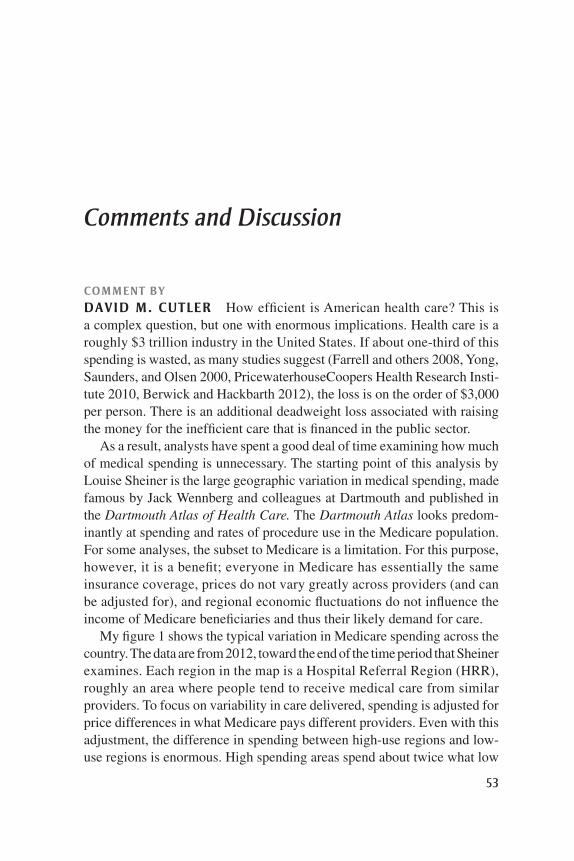
53
Comments and Discussion
Comment ByDAVID m. CUtLeR How efficient is American health care? This is a complex question, but one with enormous implications. Health care is a roughly $3 trillion industry in the United States. If about one-third of this spending is wasted, as many studies suggest (Farrell and others 2008, Yong, Saunders, and Olsen 2000, PricewaterhouseCoopers Health Research Insti-tute 2010, Berwick and Hackbarth 2012), the loss is on the order of $3,000 per person. There is an additional deadweight loss associated with raising the money for the inefficient care that is financed in the public sector.
As a result, analysts have spent a good deal of time examining how much of medical spending is unnecessary. The starting point of this analysis by Louise Sheiner is the large geographic variation in medical spending, made famous by Jack Wennberg and colleagues at Dartmouth and published in the Dartmouth Atlas of Health Care. The Dartmouth Atlas looks predom-inantly at spending and rates of procedure use in the Medicare population. For some analyses, the subset to Medicare is a limitation. For this purpose, however, it is a benefit; everyone in Medicare has essentially the same insurance coverage, prices do not vary greatly across providers (and can be adjusted for), and regional economic fluctuations do not influence the income of Medicare beneficiaries and thus their likely demand for care.
My figure 1 shows the typical variation in Medicare spending across the country. The data are from 2012, toward the end of the time period that Sheiner examines. Each region in the map is a Hospital Referral Region (HRR), roughly an area where people tend to receive medical care from similar providers. To focus on variability in care delivered, spending is adjusted for price differences in what Medicare pays different providers. Even with this adjustment, the difference in spending between high-use regions and low-use regions is enormous. High spending areas spend about twice what low

54 Brookings Papers on Economic Activity, Fall 2014
spending areas do. Put another way, if all spending moved to the level of the area at the 25th percentile of the spending distribution, overall Medi-care costs would fall by nearly one-third.
Is there anything that can justify this spending difference? That is the question Sheiner asks in this paper. Her dependent variable is basically a state-level version of my figure 1. The major difference between Sheiner’s variable and the Dartmouth Atlas measure is that Sheiner looks only at acute care, whereas my figure 1 considers post-acute care as well. Empiri-cally, a very large share of the variation in spending across areas is associ-ated with differential use of post-acute care (Institute of Medicine 2013). Nevertheless, the variation in acute care is substantial as well.
As noted, the generosity of insurance coverage is not a serious issue across areas, nor are differences in prices paid for care. What Sheiner focuses
Price-Adjusted Medicare Reimbursements (Parts A & B) per Beneficiaryby Hospital Referral Region (2012)
$10,530 to 13,600 (61)$9,910 to < 10,530 (61)$9,120 to < 9,910 (62)$8,260 to < 9,120 (61)$6,720 to < 8,260 (61)Not populated
Source: Dartmouth Institute for Health Policy and Clinical Practice. Reprinted with permission. a. Medicare reimbursements per beneficiary adjusted for age, sex, race, and price.
Figure 1. Adjusted Medicare Spending by Hospital Referral Region, 2012a

coMMentS and diScuSSion 55
on instead is health status. The areas where spending is higher are also areas where obesity rates are higher, and with them cardiovascular disease risk factors such as high cholesterol, hypertension, and diabetes.
How much of this spending difference is a true finding rather than an eco-logical error from omitting variables correlated with health status? While Sheiner does not take an absolute position on this question, on balance she argues that health status is the most likely explanation of the differences. I am skeptical that it is.
One way to test the theory is to compare the impact of disease risk at the micro and aggregate levels. The coefficients on similar disease factors tend to be very different in this exercise. Xiaohui Zhuo and others (2014) show that people with a lifetime history of diabetes spend more on health care as seniors than comparable people without diabetes, but the peak spending difference is only about twice as high. As people age, the gap narrows. In contrast, Sheiner estimates that if everyone in an area had diabetes, spend-ing would be six times higher than if no one had diabetes.
One could make the argument that the macro coefficient is larger because of measurement error in diabetes status at the micro level. But this seems implausible. The ratio of coefficients at the micro level to those at the macro level is equal to the share of variation in diabetes status at the macro level that is measured with error at the micro level. It is hard to imagine a setting where individual data would be two-thirds less precise than area-level data.
Moreover, we know more about why spending differs across geographic areas than just the fact that it does. In work I have done with colleagues (Cutler and others 2014), we analyze physician responses to vignette ques-tions about how the physician would treat particular people. In the canonical example, the vignette patient is an elderly man with very severe congestive heart failure, for whom there are essentially no restorative therapies. Empir-ically, half the men who are in the condition of this vignette patient will die within a year. Physicians express very different views about how to treat this man, with some recommending palliative care and others wanting to pur-sue aggressive intervention, even when the medical literature provides no support for the latter. These responses vary geographically, and spending is much higher in areas of the country where physicians express a preference for more aggressive care. Even with a small sample of physicians in each area, areas where more physicians wish to provide more aggressive care spend 60 percent more at the end of life. It is not the health of the patient that differs in these settings; indeed, while patient preferences about end-of-life care vary across areas, they are uncorrelated with actual end-of-life care spending. Rather, it is the view of the physician that dominates.

56 Brookings Papers on Economic Activity, Fall 2014
As Sheiner notes, in one sense this is definitive, but in another it is not. The fact that physicians have different views about optimal treatments could reflect the differing average health of patients in their areas. For example, in an area with more diabetics, physicians might decide that their guidelines should involve more aggressive care. Countering that possibility, however, are several other pieces of evidence. In addition to being correlated with health status, spending is also associated with the minority share of the pop-ulation. It is hard to know why minority race should positively influence spending, controlling for disease risk. Outside of health care, spending is correlated with measures such as the diffusion of hybrid corn technology (Skinner and Staiger 2007) and, as Sheiner shows, long-standing metrics of social capital. But where do those measures of social capital come from? The debate is in some ways endless, and Sheiner does a good job in high-lighting this.
Ultimately, we will need an intervention to tell these theories apart. Can we modify the beliefs of physicians about what is appropriate or otherwise successfully constrain their actions? If so, how?
There is another element of the issue that warrants attention. Research on waste in medical care started at the geographic level, but it has gone beyond there. It turns out that within regions, there are high-use institutions and low-use institutions. And within institutions, there are high-use departments and low-use departments. And even within departments, there are high-use clini-cians and low-use clinicians. As in a fractal, variability in medical treatments exists at every level at which it has been measured.
Consider just one example: rates at which head CT scans are ordered for patients presenting to an emergency department with atraumatic headaches. Prevedello and others (2012) examine head CT scan ordering rates among such patients at a single emergency department in a major urban hospital. The rate of such ordering varied by a factor of nearly 3:1 across physicians, from 21 percent to 60 percent.
This personalization of variability is unlikely to be due to unmeasured health status. It is hard to believe that different physicians in the same emer-gency department perceive different probabilities of brain tumors in the population as a whole. Clearly, what varies is the interpretation of how best to practice medicine.
What is most surprising about this variability is how little clinicians are aware of it. Most physicians do not know whether they are high or low utilizers of care. When alerted to their standing as a high or low utilizer, the high utilizers invariably assert that it is a consequence of differential underlying health of the patients they see, or alternatively that it reflects

coMMentS and diScuSSion 57
superior outcomes on their part. Such theories can be disproven with data. After this has occurred, physicians accept that they practice differently, and often attribute that to their training or to a particular adverse experience at some point in the past. With time and discussion, physicians can be induced to practice differently (Leonhardt 2009), but it does not happen automati-cally. It takes effort.
Most consequentially, none of this effort is rewarded. High utilization brings in more money than low utilization; head CT scans contribute posi-tively to the bottom line at most emergency departments and for many doc-tors. Organizations can spend time and money standardizing care across physicians, but there is little reason to do so if the net impact is a reduction in profitability.
This brings back the discussion of the geographic variation in care. In Atul Gawande’s (2009) famous article on McAllen, Texas, Gawande argues that physicians in McAllen have a greater taste for money relative to patient benefits than do physicians in other areas of the country. Profits and patient benefits do not always conflict, but sometimes they do. In those cases, the slope of the indifference curve between money and benefits becomes impor-tant. It is not unreasonable to believe that such trade-offs differ across phy-sicians. Nor is it unreasonable that physicians prefer to work with other physicians who have the same tastes they do. Nor is it surprising that physi-cians with preferences for profits would choose to work where patients are less healthy, which also happen to be areas where norms toward care do not significantly constrain what is done.
In this view of the world, the key issue is not the health status of the popula-tion, but the payment rules under which physicians operate. When payment is based on the amount of treatment done, physicians who value money will find that aggressive care pays. By contrast, in a more neutral reimbursement environment the variation in treatments across areas would decline. The Insti-tute of Medicine (2013) argues extensively for this view in a recent report. It concludes that the solution to geographic variation in care is not devising policies that target high-spending regions, but rather changing the payment system everywhere to reward high-value care.
The accountable care movement has picked up on this theme (Cutler 2014). One recent study estimates that 40 percent of the dollars in medical care have at least some value component to them (Catalyst for Payment Reform 2014). Many of these incentives are weak, but not all. There are more than 600 Accountable Care Organizations in operation around the country (Petersen and others 2014). Interestingly, one of the industries that is being born from this is a consulting industry to help health systems reduce

58 Brookings Papers on Economic Activity, Fall 2014
variability in care across clinicians. Addressing variability is high on the list of priorities in almost all health systems, yet most systems do not know how to do it.
The payment system is changing rapidly, and this shows every indica-tion of continuing. Thus, we are likely to know much more about some of the factors influencing physician behavior in the next few years. If Sheiner is right, the impact of these reforms on health spending will be modest—or worse, harmful. If the Gawande-Dartmouth theory is right, spending could fall without adverse impact. I look forward to the update of Sheiner’s paper, with the interim answer, when we have those results.
ReFeRenceS FoR tHe cutleR coMMent
Berwick, Donald M., and Andrew D. Hackbarth. 2012. “Eliminating Waste in U.S. Health Care.” JAMA 307, no. 14: 1513–16.
Catalyst for Payment Reform. 2014. 2014 National Scorecard on Payment Reform. San Francisco. http://www.catalyzepaymentreform.org/images/documents/ NationalScorecard.pdf
Cutler, David. 2014. The Quality Cure. University of California Press.Cutler, David, Jon Skinner, Ariel Stern, and David Wennberg. 2014. “Physician
Beliefs and Patient Preferences: A New Look at Regional Variation in Health Care Spending.” Mimeo.
Farrell, Diana, Eric Jenson, Bob Kocher, Nick Lovegrove, Fareed Melhem, Lenny Mendonca, and Beth Parish. 2008. Accounting for the Cost of US Health Care: A New Look at Why Americans Spend More. New York: McKinsey Global Insti-tute, McKinsey & Company.
Gawande, Atul. 2009. “The Cost Conundrum: What a Texas Town Can Teach Us about Health Care.” New Yorker, June 1.
Institute of Medicine. 2013. Variation in Health Care Spending: Target Decision Making, Not Geography. Washington: National Academies Press.
Leonhardt, David. 2009. “Making Health Care Better.” New York Times Magazine, November 3.
Petersen, Matthew, Paul Gardner, Tianna Tu, and David Muhlestein. 2014. Growth and Dispersion of Accountable Care Organizations. June 2014 update. Washington: Leavitt Partners.
Prevedello, Luciano M., Ali S. Raja, Richard D. Zane, Aaron Sodickson, Stuart Lipsitz, and Louise Schneider. 2012. “Variation in Use of Head Computed Tomography by Emergency Physicians.” American Journal of Medicine 125, no. 4: 356–64.
PricewaterhouseCoopers Health Research Institute. 2010. “The Price of Excess: Identifying Waste in Healthcare Spending.” New York.
Skinner, Jonathan, and Douglas Staiger. 2007. “Technology Adoption from Hybrid Corn to Beta Blockers.” In Ernst R. Berndt and Charles R. Hulten, eds., Hard-

coMMentS and diScuSSion 59
to-Measure Goods and Services: Essays in Honor of Zvi Griliches (University of Chicago Press), pp. 545–70.
Yong, P. L., R. S. Saunders, and L. A. Olsen (eds.). 2010. “The Healthcare Impera-tive: Lowering Costs and Improving Outcomes.” Workshop Series Summary from the Institute of Medicine Roundtable on Evidence-Based Medicine. Wash-ington: National Academies Press.
Zhuo, Xiaohui, Ping Zhang, Lawrence Barker, Ann Albright, Theodore Thompson, and Edward Gregg. 2014. “The Lifetime Cost of Diabetes and Its Implications for Diabetes Prevention.” Diabetes Care 37, no. 9: 2557–64.
Comment ByDoUGLAS o. StAIGeR1 Over the last four decades a large literature has documented substantial variation in health care spending, utilization, and quality across regions, hospitals, and physicians (IOM 2013, Skinner 2012). Many analysts, and the Dartmouth group in particular, argue that these dif-ferences reflect persistent productivity differences, and are not the result of random fluctuation or unmeasured differences in patient health status or preferences.
My figure 1 provides a typical example of the kind of evidence that has been produced. It plots hospital-level data on mortality and spending for Medicare patients admitted to the hospital with a heart attack (acute myo-cardial infarction, or AMI) during 2007–09. As is common in this literature, the hospital-level estimates were adjusted using standard methods to control for observed differences in patient risk and hospital prices, and hospitals with fewer than 200 AMI patients were not plotted to minimize random fluctuations (Skinner and others 2013). Nevertheless, there remains sub-stantial variation across hospitals: average 1-year Medicare expenses range from $30,000 to $60,000, while 1-year mortality rates range from 20 per-cent to 45 percent. Compared to the most productive hospitals (indicated by the scatterplot points in the lower left of the figure), patient mortality and expenditures are roughly a third higher in the least productive hospitals (upper right).
The key features of my figure 1—twofold variation in cost and qual-ity, which are largely unrelated to each other, implying large variation in productivity—are not unique to this example. Similar results have been
1. I thank Amitabh Chandra, Jonathan Skinner, and James Feyrer for helpful comments and advice. I am co-founder of, have an equity interest in, and have consulted for ArborMetrix, a company that sells performance measurement systems and consulting services to insurers and hospitals.

60 Brookings Papers on Economic Activity, Fall 2014
found across different levels of aggregation (county, state, hospital, physi-cian) using a wide variety of data sets and patient populations. In fact, persis-tent productivity differences are not unique to health care. A long literature has documented similarly large productivity differences across plants and firms (Syverson 2011), teachers and schools (Jackson, Rockoff, and Staiger 2014) and countries (Klenow and Rodríguez-Clare 1997). In health care, as in these other settings, there is a growing consensus that these differences are in large part causal and capture how average costs and outcomes would change if a patient were to be treated in a different region or by a different provider. Much of the recent literature has moved on to understanding why these productivity differences exist and developing strategies that would encourage less efficient providers and regions to move, in Peter Orszag’s
0.45
0.40
0.35
0.30
0.25
40,00035,000 45,000
Risk- and price-adjusted Medicare expenditures (dollars)b
50,000 55,000 60,000
Risk-adjusted 1-year mortalityb
Source: Author’s calculations, using data from Skinner and others (2013).a. The figure plots risk-adjusted mortality rates against risk- and price-adjusted 1-year Medicare expendi-
tures (dollars) for each hospital, based on Medicare beneficiaries age 65 or over admitted for an acute myocardial infarction (AMI) from 2007 to 2009. Only hospitals with at least 200 Medicare AMI admissions are plotted.
b. Risk and price adjustment were done using standard patient-level methods; risk adjustment did not control for Medicare’s Hierarchical Condition Categories (HCCs). See Skinner and others (2013).
Figure 1. Spending and Mortality for AMi Admissions, by Hospital, 2007–09a

coMMentS and diScuSSion 61
words, toward “the proven and successful practices adopted by lower-cost areas and hospitals” (Orszag 2009).
In the paper under discussion here, Louise Sheiner takes a step back to challenge this consensus. She argues that geographic variation in health care spending reflects unmeasured population health needs and socioeconomic characteristics rather than causal productivity differences. Her key piece of evidence, illustrated in her figure 1, is that there is a strong correlation between average Medicare spending in a state and proxies for health needs in the state such as the share of the state that is diabetic. This correlation, she argues, is prima facie evidence that geographic variation is driven primarily by differences in population health needs, not differences in productivity. After she controls for the share of the state that is diabetic and a few other state-level measures of socioeconomic status, little unexplained variation remains. More broadly, Sheiner argues that it is difficult to learn anything from geographic variation, because high-spending states differ in multiple dimensions from low-spending states.
It is not clear what we learn from the correlations documented by Sheiner. Earlier work has found similar correlations of population health and demo-graphic measures with health care spending and quality, but the interpreta-tion of these correlations has varied. For example, Richard Cooper (2009) documents a strong correlation between regional spending and poverty and, like Sheiner, has argued that regional variation reflects health needs rather than productivity differences. Alternatively, a number of papers have found higher mortality and adverse event rates in hospitals serving minor-ity populations, and interpreted this as evidence that true quality of care is lower in minority-serving hospitals (Morales and others 2005, Skinner and others 2005, Lake and others 2015). Amitabh Chandra and Staiger (2007) find that areas with the types of heart attack patients most appropriate for aggressive treatment are more likely to provide aggressive treatment to all patients, but argue that this is the result of true productivity differences in regions that specialize in providing aggressive treatment. Jonathan Skinner and Staiger (2007) also find strong correlations at the state level between health care spending and mortality (for Medicare AMI patients) and a wide variety of demographic measures and proxies for innovativeness in the state, but they interpret the data as suggesting that true productivity dif-ferences are related to state-level barriers to adoption of efficient tech-nologies (see also Skinner and Staiger 2015).
Are these correlations driven by unmeasured health differences across areas, as Sheiner and Cooper both argue, or is there simply a correlation between true productivity differences and state population characteristics,

62 Brookings Papers on Economic Activity, Fall 2014
as much of the recent literature argues? A simple empirical framework that relates the standard patient-level estimation method to Sheiner’s state-level estimation method helps to clarify why the state-level correlations docu-mented by Sheiner cannot answer this question.
The standard risk-adjustment method runs a patient-level fixed-effect regression of the form
(1) ˆ ˆ ˆ ,1= β + α + εY Xij ij j ij
where Yij is a patient outcome (such as spending or mortality) for patient i treated in region (or hospital) j, and Xij is a vector of patient-level controls such as age, gender, race, pre-existing medical conditions and, in some data sets, detailed clinical characteristics. Estimates of the fixed effects ˆ( )α j are the risk-adjusted measures of patient spending or mortality in each region or hospital (such as what was plotted in my figure 1). These measures may be associated with average characteristics of patients ( )Xj or other charac-teristics (Zj) of the region:
�(2) ˆ ˆ ˆ .2 3α = β + β + ωX Zj j j j
Averaging my equation 1 at the state level and substituting for α̂ j using my equation 2 yields Sheiner’s between-state estimator:
�(3) ˆ ˆ ˆ .1 2 3( )= β + β + β + ωY X Zj j j j
Sheiner argues that the residual from this regression �( )ω j is a better esti-mate of the causal variation in productivity across states than the residual from my equation 1 ˆ( )α j . Thus, the key to understanding the difference between the standard approach and Sheiner’s approach is my equation 2: Sheiner believes that the correlation between α̂ j and the regional measures
,( )X Zj j is due to health attributes that were omitted from my equation 1 and removes it, whereas the standard approach treats α̂ j as true productiv-ity estimates and tries to understand why productivity is correlated with the regional measures. Estimates of my equation 2 (or equivalently, Sheiner’s equation 3) provide no evidence to decide which interpretation is correct. Therefore, the state-level correlations documented by Sheiner cannot answer the key question of whether regional and provider variation is informative about productivity.
Other evidence, however, strongly suggests that regional and provider-level variation is not driven by omitted health attributes. First, regional and hospital-level estimates that control for more detailed clinical information

coMMentS and diScuSSion 63
at the patient level are highly correlated with standard estimates, and they continue to be correlated with population characteristics such as income and race (Dimick and Birkmeyer 2008, Dimick and others 2010, McClellan and Staiger 2000, Morales and others 2005, Skinner and others 2005, Sutherland, Fisher, and Skinner 2009). Second, there is substantial varia-tion across regions and hospitals in measures for which health attributes are not relevant, such as aspirin and beta blocker use in the hospital fol-lowing a heart attack, and these measures are also strongly correlated with population characteristics such as income and race (Baicker and Chandra 2004, Skinner and Staiger 2007). Third, there is substantial variation across regions in how physicians say they would treat patients in standardized vignettes (holding patient attributes constant), and this variation is strongly correlated with actual practice patterns (Cutler and others 2013). Finally, two seminal papers from the Dartmouth group (Fisher and others 2003a and 2003b) focus on regional differences in end-of-life spending because it “reflects the component of regional variation in Medicare spending that is unrelated to regional differences in illness” (p. 273). They find that health status is similar across regions with different end-of-life spending, but patients received roughly 60 percent more care in the higher-spending regions.
More importantly, there is growing evidence that regional and provider variation in spending and patient outcomes are related to causal estimates of productivity differences. First, there are large impacts on average costs when patients are randomized to medical groups (Doyle, Ewer, and Wagner 2010) or quasi-randomized to hospitals (Doyle 2011, Doyle and others 2015), and these differences are strongly predicted by standard risk-adjusted estimates. Second, Amy Finkelstein, Matthew Gentzkow, and Heidi Williams (2014) find that when Medicare patients move from one region to another, their Medicare spending and utilization change immediately by an amount that is roughly 50 to 60 percent of the difference in average spending and utilization between the regions. Consistent with Jason Sutherland, Elliott Fisher, and Jonathan Skinner (2009), they find that health characteristics can explain only about a third of the average differences in spending and utili-zation across regions. Finally, John Birkmeyer and others (2013) directly assesses surgical technical skill using video, and find that surgeon skill was strongly negatively associated with risk-adjusted patient complication rates and subsequent rates of reoperation, readmission, and emergency room admission.
All of this evidence suggests that standard patient-level risk-adjusted measures of spending, utilization, and quality are to a large extent capturing

64 Brookings Papers on Economic Activity, Fall 2014
causal productivity differences across regions and providers rather than omitted health attributes of the population. This would suggest that Sheiner is finding a correlation between true productivity differences and state pop-ulation characteristics, and misinterpreting it as evidence of omitted health attributes.
This view of Sheiner’s results is consistent with a broader literature arguing that micro-founded estimates of productivity are valid, and that macro-level correlations of productivity with population characteristics are difficult to interpret. For example, in the field of education, so-called value-added esti-mates of teacher performance (based on student-level test score regressions similar to my equation 1) have been validated in a number of natural and ran-domized experiments (Bacher-Hicks, Kane, and Staiger 2014, Chetty, Fried-man, and Rockoff 2014a, 2014b, Kane and Staiger 2008, Kane and others 2013), despite the fact that these estimates are strongly correlated with aver-age student poverty. Macroeconomists have abandoned production function estimates based on cross-country variation (which, like Sheiner’s cross-state regressions, explain away most of the variation), and instead use estimates of total factor productivity based on micro-founded estimates of the returns to physical and human capital (Klenow and Rodríguez-Clare 1997).
The important question is not whether large and persistent productivity differences exist—the evidence is overwhelming that they do. The impor-tant question is why these productivity differences exist, why they are asso-ciated with a number of market and firm characteristics, and whether there are strategies that could improve productivity and welfare. As Sheiner notes, and as has become apparent in the macro literature on productivity, simple correlations between productivity and market characteristics are not likely to take us very far. Instead, we need models that can explain persistent produc-tivity differences, empirical tests of these models, and evaluations of inter-ventions designed to improve productivity. Along these lines, recent work on productivity spillovers (Chandra and Staiger 2007), technology diffusion (Skinner and Staiger 2015), competition (Bloom and others 2010, Chandra and others 2013), and management quality (Bloom and others 2014) are a promising step forward toward a better understanding of why these differ-ences exist. Running cross-section regressions of state-level spending on state-level health measures, as Sheiner does, is a step backwards.
ReFeRenceS FoR tHe StAigeR coMMent
Bacher-Hicks, Andrew, Thomas Kane, and Douglas Staiger. 2014. “Validating Teacher Effect Estimates Using Changes in Teacher Assignments in Los Angeles.” Work-ing Paper no. 20657. Cambridge, Mass.: National Bureau of Economic Research.

coMMentS and diScuSSion 65
Baicker, Katherine, and Amitabh Chandra. 2004. “Medicare Spending, the Physician Workforce, and Beneficiaries’ Quality of Care.” Health Affairs, April.
Birkmeyer, John, Jonathan Finks, Amanda O’Reilly, Mary Oerline, Arthur Carlin, Andre Nunn, Justin Dimick, Mousumi Banerjee, and Nancy Birkmeyer. 2013. “Surgical Skill and Complication Rates after Bariatric Surgery.” New England Journal of Medicine 369, no. 15: 1434–42.
Bloom, Nicholas, Carol Propper, Stephan Seiler, and John Van Reenen. 2010. “The Impact of Competition on Management Quality: Evidence from Public Hospi-tals.” Working Paper no. 16032. Cambridge, Mass.: National Bureau of Economic Research.
Bloom, Nicholas, Raffaella Sadun, Renata Lemos, Daniela Scur, and John Van Reenen. 2014. “The New Empirical Economics of Management.” Occasional Paper no. CEPOP41. London School of Economics and Political Science, Center of Economic Performance.
Chandra, Amitabh, Amy Finkelstein, Adam Sacarny, and Chad Syverson. 2013. “Healthcare Exceptionalism? Productivity and Allocation in the U.S. Health-care Sector.” Working Paper no. 19200. Cambridge, Mass.: National Bureau of Economic Research.
Chandra, Amitabh, and Douglas Staiger. 2007. “Productivity Spillovers in Health-care: Evidence from the Treatment of Heart Attacks.” Journal of Political Economy 115, no. 1: 103–40.
Chetty, Raj, John Friedman, and Jonah Rockoff. 2014a. “Measuring the Impacts of Teachers I: Evaluating Bias in Teacher Value-Added Estimates.” American Economic Review 104, no. 9: 2593–32.
———. 2014b. “Measuring the Impacts of Teachers II: Teacher Value-Added and Student Outcomes in Adulthood.” American Economic Review 104, no. 9: 2633–79.
Cooper, Richard. 2009. “States with More Health Care Spending Have Better-Quality Health Care: Lessons about Medicare.” Health Affairs 28, no. 1: w103–w115.
Cutler, David, Jonathan Skinner, Ariel Dora Stern, and David Wennberg. 2013. “Physician Beliefs and Patient Preferences: A New Look at Regional Varia-tion in Health Care Spending.” Working Paper no. 19320. Cambridge, Mass.: National Bureau of Economic Research.
Dimick, Justin, and John Birkmeyer. 2008. “Ranking Hospitals on Surgical Qual-ity: Does Risk-Adjustment Always Matter?” Journal of the American College of Surgeons 207, no. 3: 347–51.
Dimick, Justin, Nicholas Osborne, Bruce Hall, Clifford Ko, and John Birkmeyer. 2010. “Risk Adjustment for Comparing Hospital Quality with Surgery: How Many Variables Are Needed?” Journal of the American College of Surgeons 210, no. 4: 503–08.
Doyle, Joseph. 2011. “Returns to Local-Area Healthcare Spending: Using Health Shocks to Patients Far from Home.” American Economic Journal: Applied Economics 3, no. 3: 221–43.

66 Brookings Papers on Economic Activity, Fall 2014
Doyle, Joseph, Steven Ewer, and Todd Wagner. 2010. “Returns to Physician Human Capital: Evidence from Patients Randomized to Physician Teams.” Journal of Health Economics 29, no. 6: 866–82.
Doyle, Joseph, John Graves, Jonathan Gruber, and Samuel Kleiner. 2015. “Mea-suring Returns to Hospital Care: Evidence from Ambulance Referral Patterns.” Journal of Political Economy, forthcoming.
Finkelstein, Amy, Matthew Gentzkow, and Heidi Williams. 2014. “Sources of Geographic Variation in Health Care: Evidence from Patient Migration.” Working Paper no. 20789. Cambridge, Mass.: National Bureau of Economic Research.
Fisher, Elliott, David Wennberg, Therese Stukel, Daniel Gottlieb, F. L. Lucas, and Etoile Pinder. 2003a. “The Implications of Regional Variations in Medicare Spending. Part 1: The Content, Quality, and Accessibility of Care.” Annals of Internal Medicine 138, no. 4: 273–87.
———. 2003b. “The Implications of Regional Variations in Medicare Spending. Part 2: Health Outcomes and Satisfaction with Care.” Annals of Internal Medi-cine 138, no. 4: 288–98.
IOM (Institute of Medicine). 2013. “Variation in Health Care Spending: Target Decision Making, Not Geography.” Washington: National Academies Press.
Jackson, Kirabo, Jonah Rockoff, and Douglas Staiger. 2014. “Teacher Effects and Teacher-Related Policies.” Annual Review of Economics 6: 801–25.
Kane, Thomas, Daniel McCaffrey, Trey Miller, and Douglas Staiger. 2013. “Have We Identified Effective Teachers? Validating Measures of Effective Teaching Using Random Assignment.” MET Project Research Paper, Bill & Melinda Gates Foundation.
Kane, Thomas, and Douglas Staiger. 2008. “Estimating Teacher Impacts on Stu-dent Achievement: An Experimental Evaluation.” Working Paper No. 14607. Cambridge, Mass.: National Bureau of Economic Research.
Klenow, Peter, and Andres Rodríguez-Clare. 1997. “The Neoclassical Revival in Growth Economics: Has It Gone Too Far?” In NBER Macroeconomics Annual 1997, ed. by Ben Bernanke and Julio Rotemberg. Cambridge, Mass.: National Bureau of Economic Research.
Lake, Eileen, Douglas Staiger, Jeffrey Horbar, Michael Kenny, Thelma Patrick, and Jeannette Rogowski. 2015. “Disparities in Perinatal Quality Outcomes in Very Low Birth Weight Infants in Neonatal Intensive Care.” Health Services Research, forthcoming.
McClellan, Mark, and Douglas Staiger. 2000. “Comparing the Quality of Health Care Providers.” In Frontiers in Health Policy Research, vol. 3, ed. by Alan Garber. MIT Press.
Morales, Leo, Douglas Staiger, Jeffrey Horbar, Joseph Carpenter, Michael Kenny, Jeffery Geppert, and Jeannette Rogowski. 2005. “Mortality among Very Low Birthweight Infants in Hospitals Serving Minority Populations.” American Journal of Public Health 95, no. 12: 2206–12.
Orszag, Peter. 2009. “Health Costs Are the Real Deficit Threat.” Wall Street Journal, May 15.

coMMentS and diScuSSion 67
Skinner, Jonathan. 2012. “Causes and Consequences of Geographic Variation in Health Care.” In Handbook of Health Economics, vol. 2, ed. by T. McGuire, M. Pauly, and P. Pita Baros. North Holland.
Skinner, Jonathan, Amitabh Chandra, Douglas Staiger, Julie Lee, and Mark McClellan. 2005. “Mortality after Acute Myocardial Infarction in Hospitals That Disproportionately Treat Black Patients.” Circulation 112: 2634–41.
Skinner, Jonathan, and Douglas Staiger. 2007. “Technology Adoption from Hybrid Corn to Beta Blockers.” In Hard-to-Measure Goods and Services: Essays in Honor of Zvi Grilliches, ed. by Ernst R. Berndt and Charles R. Hulten. Univer-sity of Chicago Press and NBER.
———. 2015. “Technology Diffusion and Productivity Growth in Health Care.” Review of Economics and Statistics, forthcoming.
Skinner, Jonathan, Weiping Zhou, Daniel Gottlieb, and Elliott Fisher. 2013. “Mea-suring Hospital-Level Healthcare Expenditures and Outcomes with Disease-Specific Cohorts.” Final Report for the Institute of Medicine Committee on Geographic Variation in Health Care Spending, January 10.
Sutherland, Jason, Elliott Fisher, and Jonathan Skinner. 2009. “Getting Past Denial—The High Cost of Health Care in the United States.” New England Journal of Medicine 361: 1227–30.
Syverson, Chad. 2011. “What Determines Productivity?” Journal of Economic Literature 49, no. 2: 326–65.
GeneRAL DISCUSSIon Peter Orszag agreed with discussant David Cutler that even without emphasizing the role of regional variation one must conclude that there is a massive amount of variation in the practice norms in health care and that risk adjustments do not explain it. In fact, hospitals are hiring businesses to examine their practices and identify risk-adjusted clinical variation to reduce wasteful practices, something that would make no sense to do if all the treatment variation stemmed from the riskiness of the patients alone. This approach is becoming more promi-nent for two reasons. First, hospitals had little incentive to do it as long as they did not face capitated or other risk-based payment systems; however, the reality and, more importantly, the perception now is that the payment system is evolving away from fee-for-service payments. Second, digitiza-tion of medical records makes these analyses easier to do than in a paper-based system.
Orszag wondered how variations in cost relate to treatment quality. He cited a series of studies done by Joseph Doyle and his colleagues. Their initial paper suggested that higher-cost hospitals showed lower mortality rates one year after acute-care treatment, but that paper focused only on emergency room visits. When an updated version of the analysis looked

68 Brookings Papers on Economic Activity, Fall 2014
at all acute care and post-acute care as well, it found the correlation with mortality to be zero; there was a positive correlation for acute care and a negative one for post-acute spending, and when total treatment spending was examined it found no correlation at all. So putting together the fact that there is huge variation both among hospitals and also within each hospital, and given the finding—albeit based on limited evidence to date—that there is no clear connection between treatment cost and quality of outcomes, this seems to take one to the same conclusion that the Dartmouth research has found, albeit in a different way and at a different level of aggregation.
Amanda Kowalksi voiced her enthusiasm for the big data revolution and its application to discerning individual results in health care and, par-ticularly, the Affordable Care Act (ACA). She felt too that if individual-level data are becoming available they are likely to reveal much more than is possible with state-level data, noting that the Medicare claims data have been analyzed at the individual level for some time now and were the foundation of the Dartmouth project’s work. It surprised her that Louise Sheiner was able to run state-level regressions and find patterns that individual-level analyses had been unable to find.
She wondered if the variation Sheiner found could be explained by comparing the R-squareds from a state-level regression to those from an individual-level regression. Taking blood pressure as an example, on the individual level there would be much more variation than there would be at the state level, since the mean would average that out. She asked Sheiner whether she had tried inserting state-level controls into the individual-level regressions and, if she had, whether the findings still held.
Sheiner responded to Kowalski’s last question by affirming that the findings had in fact held up quite well after testing the individual data with state-level controls.
Drawing an analogy to a field he was more familiar with, Steven Davis mentioned that a large literature documents performance differences, usu-ally in total factor productivity, across plants in the manufacturing sector. In addition to enormous performance heterogeneity, the literature also finds that better-performing units tend to grow at the expense of worse-performing units. Unlike the health care sector, in manufacturing there are strong market incentives to perform well, and there is not the same kind of moral hazard and adverse selection as in the health care sector. Nevertheless, the manufacturing sector shows very large and somewhat persistent performance differences across plants. In that light, it would be quite surprising if hospitals and other units in the health care sector did not show equally large or larger performance differences.

coMMentS and diScuSSion 69
Picking up on the medical management aspect of the paper, Davis noted that recent descriptive studies of health care management by Nicholas Bloom and others find that even basic management 101 training can improve performance outcomes. Their findings reinforce what Cutler said in his remarks about the benefits of showing physicians how their peers handle similar patients. The literature also points to the difficulty of achieving performance gains in this way due to the resistance people have to changing their own workplace habits. Health practitioners have to be walked through alternative approaches step by step to be convinced to change, and this takes a lot of data and a lot of time. In sum, he felt that while there are large performance gains to be had in the health care sec-tor, there are good reasons to think it will take a lot of work and time to achieve them.
Caroline Hoxby disagreed with discussant Douglas Staiger’s character-ization of the literature on the role of value-added in teacher performance. The literature actually found that even within a single school there are enor-mous variations, and some of the highest-spending areas in the country were found to have poor quality teachers as measured by value-added, while some low-spending areas were found to have teachers with high value-added. For example, regressing average value-added in a school district or state on a lot of aggregate characteristics, one finds the regressions do not explain much, whereas the average characteristics of the district or state do a par-ticularly good job of explaining average value-added. This is one of the reasons, she believes, why the differences among teachers in their produc-tivity probably stem from some aspect of what each teacher is doing and not just from some omitted variable.
Hoxby found Sheiner’s omitted-variable explanation for why the state characteristics matter completely plausible. If one knows a variable at the individual level, knowing the aggregate variable will also be valuable, since it can tell us whether our individual measure has a lot of measure-ment error. For example, if one wants to know someone’s permanent income, knowing that his income is x this year is not very informative until one also knows the typical income of his neighborhood. The median income of all of his neighbors probably says a lot about his permanent income. The same thing could be true in health. After people get a diag-nostic test, researchers cannot normally follow them day by day to see what they are doing. Instead, researchers have a lot of imperfect measures of their health, which are used to make risk adjustments. It is not surprising that putting those risk adjustment measures in context enables us to learn a lot more about what their risks are.

70 Brookings Papers on Economic Activity, Fall 2014
Hoxby opined that the health literature may suffer from relatively poor quality in the data it relies on. Unlike analyses in education, where the key control variable in studying teachers’ effectiveness can be their stu-dents’ performance the previous year, in health care individual outcomes cannot be measured very often. One cannot observe individuals dying of heart disease “over again” every year. Doing individual risk adjustments in health studies is like trying to control for risk in a study of teachers’ effectiveness but only being able to observe their students’ height or race, rather than the most important variable, which would be the students’ per-formance at the end of the last year.
John Haltiwanger elaborated on a few points that Davis and Staiger raised concerning the productivity literature. Studies have found enormous heterogeneity in productivity across firms within every narrowly defined industry, and he saw no reason to expect health care to be an exception. An open question is this: What prevents resources being moved away from the low-productivity firms to the high-productivity firms? Studies need to be structured to distinguish between frictions—like market structure and product differentiation—and distortions. Frictions support productiv-ity dispersion in an equilibrium even if there are no distortions, and this should be true of the health care industry as well. This paper appears to take the view that dispersion in productivity is an indicator of distortions. But that needs to be verifed more directly. In the productivity literature, there is an active research agenda looking for direct measures of such dis-tortions, either in cross-section or over time. That same approach should be used in this context to try to understand the dispersion in health care productivity and quality.
Justin Wolfers wanted to know if Staiger, whom he thought had mounted a stout defense of the view that the hospital cross-state variation was mostly causal, could explain why any of that would also be correlated with percent diabetic. Is there an explanation that can square all the facts including those, like the diabetes patterns, that seem so central to Sheiner’s argument?
Robert Gordon felt that Sheiner’s paper offered a wonderful new set of insights. Her series of scatter-plot graphs made him think immediately of the Old Confederacy and specifically the Mississippi Delta cotton belt, which had the highest share of black share croppers in the history of Jim Crow and the lowest literacy rates. There are two different correlations with the racial effect of being black in America: on health and on poverty. The list of health problems that blacks and low-income Americans are more prone to includes diabetes, cancer, and many other diseases.

coMMentS and diScuSSion 71
And yet, Gordon added, geography is not destiny. During the Great Migration, as many as 2,000 African Americans arrived by train each day in Chicago alone, all coming up from the Deep South. Many of them set-tled in the South Side of Chicago, and for over 45 years that population has been truly different in its health statistics. So the health patterns follow the racial group, not the region per se.
This may also beg the question of why health status is negatively cor-related with economic growth, rather than positively correlated. Gordon suggested three historical reasons. First, the invention of air conditioning, which encouraged population growth in lower-wage states, such as Arizona. Second, the Taft-Hartley Act, which introduced the right of southern states to avoid unions, again keeping wages low. And third, the slowing down of the demand curve for labor. An example of the last factor is the recent deci-sion by Electrolux to abandon a factory in Pennsylvania and build the most advanced refrigerator factory in the world outside of Memphis, which is still one of the poorest cities in the country. All of these factors have encour-aged a lopsided geographic pattern of economic growth, so much so that the state-based economic growth rates in low-wage states have outpaced the rates in high-wage states by four to one.
Louise Sheiner responded, first, by agreeing with the point that with so many factors being so closely correlated it is hard to pick out what is causal. She agreed with Staiger that the racial variable—percent black—is not causal but rather is associated with other factors. In her view the geographic locations are genuinely different, and this makes the analysis very difficult. Referring to Cutler’s vignette research, which illustrated health practice styles, she agreed that these styles vary across areas, as do measures of mean health in each place.
This presents a problem with every individual-level regression, in her view, because if a locality’s mean health is what actually matters, one cannot find that using the individual regressions. A more important chal-lenge, in her view, is to understand what causes the differences in practice styles across areas. If it is differences in social capital—and she believes it probably is—this becomes tricky to capture, because social capital affects so many things. Places where doctors make good decisions have to have good social capital, but they also have very healthy patients making good decisions. Therefore, simply running a regression about doctors’ styles and health spending may indeed show a close relationship between the two, but the cause might not be the practice styles.
Responding to Cutler’s skepticism that diabetes could be such a sig-nificant factor in health costs, inasmuch as costs would be 600 percent

72 Brookings Papers on Economic Activity, Fall 2014
higher if everyone in a population were diabetic, she said that in fact the differences between Minnesota and Mississippi, where diabetes rates are 6 percent versus 12 percent, do support this. If one increased the share of the adult population that is diabetic from 6 percent to 12 percent, then the regression coefficient shows that total health spending would go up about 40 percent, which seems quite plausible, given the roughly 50 percent dif-ference in life expectancy at age 65 between Minnesota and Mississippi.
The enormous amount of health spending in the South is incredibly inefficient, Sheiner said. There simply should not be so many people so sick, so this indicates a large, societal problem. The policy question con-cerns whether this is an inefficiency that will be easy to change. Could the passage of a few laws and other changes allow us to quickly save 30 percent on Medicare? Of course it will not be that easy, just as it is not reasonable to think that changes in educational policy are likely to raise achievement and wages in Mississippi to the levels they are at in Minnesota—although that would be wonderful.
Sheiner asked everyone to consider the fact that the health patterns have been so stable across time. Consider too the fact that Kaiser Perman-ente, which she believes has all the right incentives and could have made all the right changes in practice styles and taken over the market—since after all Kaiser has been both lower-cost and higher-quality—nevertheless has not managed to do that. This tells us that making progress is not going to be easy.