wibe de jong devesh tiwari lawrence berkeley national

Robust and Resource-EfficientQuantum Circuit ApproximationTirthak Patel

Northeastern UniversityBoston, Massachusetts, USA

Ed YounisLawrence Berkeley National

LaboratoryBerkeley, California, USA

Costin IancuLawrence Berkeley National


Wibe de JongLawrence Berkeley National


Devesh TiwariNortheastern University

Boston, Massachusetts, USA

ABSTRACT

We present QEst, a procedure to systematically generate approx-imations for quantum circuits to reduce their CNOT gate count.Our approach employs circuit partitioning for scalability with pro-cedures to 1) reduce circuit length using approximate synthesis,2) improve fidelity by running circuits that represent key samplesin the approximation space, and 3) reason about approximationupper bound. Our evaluation results indicate that our approach of“dissimilar” approximations provides close fidelity to the originalcircuit. Overall, the results indicate that QEst can reduce CNOTgate count by 30-80% on ideal systems and decrease the impact ofnoise on existing and near-future quantum systems.

1 INTRODUCTION AND MOTIVATION

We begin by providing a brief relevant background of quantumcomputing, followed by motivation for QEst, and summarize theapproach and contributions of QEst.

1.1 Quantum Computing: A Brief Background

The unit of information in quantum computing is the qubit. Thisis a two-level abstraction, whose state is represented by |𝜓 ⟩ =

𝛼 |0⟩ + 𝛽 |1⟩, which is a superposition of the |0⟩ and |1⟩ states.When this qubit is measured, its superposition collapses and it canbe measured in state |0⟩ with probability ∥𝛼 ∥2 and in state |1⟩ withprobability ∥𝛽 ∥2, such that ∥𝛼 ∥2 + ∥𝛽 ∥2 = 1. Similarly, an 𝑛-qubitentangled quantum system can be represented as a superposition

of 2𝑛 states: |𝜓 ⟩ =𝑘=𝑛−1∑︁𝑘=0

𝛼𝑘 |𝑘⟩, such that𝑘=𝑛−1∑︁𝑘=0∥𝛼𝑘 ∥2 = 1.

Under Deutch’s computational model, a quantum program canbe represented as a circuit of operations [9]. A quantum systemcan be put into a desired superposition state using quantum gatesor operations. For example, a one-qubit NOT operation can beused to rotate the state of qubit (|0⟩ to |1⟩ or vice versa), whilea two-qubit controlled-NOT or CNOT operation can be used toentangle two qubits and apply a NOT gate to the “target” qubitif the “control” qubit is in the |1⟩ state. When these operationsare applied in succession to one another, they form a “quantumcircuit” that represents and executes the corresponding “quantumalgorithm.” Note that all quantum algorithms can be represented asa sequence of one-qubit rotation gates and two-qubit CNOT gates.

10 20 30 40 50 60 70 80 90 100Timestep

0.8

0.9

1.0

Ave

rage

Mag

net

izat

ion

Ground Truth

Current Approach (Qiskit)

(a) TFIM

5 10 15 20 25 30 35 40 45 50Timestep

−0.5

0.0

0.5

Sta

gger

edM

agn

etiz

atio

n

Ground Truth

Current Approach (Qiskit)

(b) Heisenberg

Figure 1: The output of the TFIM and Heisenberg quan-

tum algorithms on the IBMQ Manila quantum computer

using all Qiskit compiler optimizations (current approach)

is far from the expected output (ground truth) at different

timesteps.

1.2 Motivation for QEst

Existing quantum systems and projected near-term future quantumsystems suffer from a pack of different types of errors [20, 32].These include state-preparation and measurement (SPAM) errorsand qubit state decoherence errors. These near-term intermediate-scale quantum (NISQ) devices also suffer from errors related toapplying one-qubit and two-qubit gates to a qubit. These errorsget compounded over the course of a quantum circuit, as a circuitruns many quantum operations. The two-qubit (CNOT) operationerror rate (1-3%) tends to be an order of magnitude above one-qubitoperation error rate.

This makes it difficult to run long quantum circuits with manyCNOT gates on near-term quantum computers as the CNOT gateshave a high application error as well as take longer to apply, causingdecoherence errors. Previous works have proposed several tech-niques that focus on circuit compilation and mapping to hardwarein a manner that reduces the CNOT gate count of the circuit as wellas reduces the impact of the errors. These include reducing gatecount by collapsing adjacent gates, deleting gate operations usingcommutativity and unitary laws, reducing the number of CNOTand SWAP operations (implemented using three CNOT gates) byperforming layout-aware mapping of the quantum circuit to thehardware, and performing noise-aware mapping to ensure thatmore noisy qubits and operations are avoided as much as possi-ble [21, 26, 27, 35, 37, 39, 42, 44, 45]. Qiskit [25], IBMQ’s python-based quantum compiling package has these state-of-the-art com-pilation techniques implemented as optimization passes, whereby

arX

iv:2

108.

1271

4v1

[qu

ant-

ph]

28

Aug

202

1

arXiv, August, 2021 Tirthak Patel, Ed Younis, Costin Iancu, Wibe de Jong, and Devesh Tiwari

the optimizations are applied one after another. While these compi-lation and mapping passes are effective in some cases, they are notable to reduce the gate count to a degree that is able to reduce thenoise sufficiently.

As an instance, Fig. 1(a) and (b) show the output of the TFIM(Transverse Field Ising Model) and Heisenberg quantum algorithms,respectively, in the ideal (ground truth) scenario vs. the case inwhich they are on run on the real IBMQ Manila quantum com-puter [6]. TFIM outputs the time evolution of the average magne-tization (energy) of a four-spin physical system with only the 𝑧Hamiltonian interaction component, while Heisenberg outputs thetime evolution of a four-spin system with 𝑥,𝑦, 𝑧 Hamiltonian inter-action components [3]. Even though the IBMQ Manila computer isa relatively low-error NISQ device and all of the Qiskit compiler op-timizations are applied when running the circuit on the computer,the output is far from the expected ideal output. The error is largeenough for the output to be not provide meaningful insights. Forexample, with TFIM, the output does not remain consistent acrossthe timesteps (even though it should according to the ground truthoutput), not does it have the same magnetization amplitude as theground truth.

1.3 Approach and Contributions of QEst

Overall, the compilation and mapping passes employed by the state-of-the-art approaches cannot reduce the output error sufficiently.Therefore in this work, we present QEst, a technique that focuseson delivering a large reduction in CNOT gate count to reduce theeffect of noise.

QEst is built on are a few key observations and opportunities.A quantum circuit can be mathematically represented as a unitarymatrix. A unitary matrix can have multiple mathematically close“approximations”. These approximated unitaries can represent theoriginal circuit’s functionality. QEst leverages this property todemonstrate that it is possible to use approximations to our advan-tage to improve the output fidelity of complex quantum programson erroneous NISQ devices.

While the idea of approximating circuits appears promising, itposes multiple challenges not solved by prior works before it can berealized in practice. First, approximating a complex quantum circuitrequires calculating approximate circuits of a large unitary matrix.Unfortunately, the calculation of how mathematically approximatea circuit is to its original circuit is computationally infeasible forquantum programs beyond four-five qubits. QEst employs circuitpartitioning to make the problem tractable: QEst applies approxi-mations on small-size partitions (blocks) and then, combines theseapproximate blocks to produce an approximate full circuit for theoriginal circuit. While this is the only way to produce approxima-tions for large circuits, it poses two primary challenges.

(1) First, when we combine multiple approximate circuit blocksto produce a full approximate circuit, there is no existing knowledgeor mechanism to understand how these approximations interactand affect the overall quality of the full approximate circuit. QEstovercomes this hurdle by providing a theoretical proof to guaranteethat the quality of the approximation of the full circuit can be boundedby controlling the quality of the approximations of blocks. This allows

QEst to combine the approximate blocks and guarantee that theoverall approximation is of an acceptable quality.

(2) The second challenge is that the quality of a circuit approxi-mation is expressed as the difference between the unitary matrix ofthe original circuit and unitary matrix generated after approxima-tion; this measure of approximation does not have strict ordering ordirect analytical relationship with the output fidelity. Thus, differ-ent “similar” approximate circuits can potentially produce differentprogram outputs (and hence, output fidelities). QEst overcomesthis challenge by devising a novel apriori selection and combinationstrategy to indirectly control the overall output fidelity by choosinga set of “dissimilar” approximate circuits that have low CNOT gatecounts. QEst’s method is effective in achieving higher output fidelityby controlling the approximations for individual circuits.

The main contributions of this work are as following:

• QEst leverages the approach of circuit synthesis, a techniqueto generate a mathematically equivalent circuit for a givenquantum circuit [8, 13, 14, 23, 34], and approximates it togenerate low-CNOT-gate-count circuits that deliver a largereduction in noise.• QEst defines an apriori approximation selection criterionthat enables it to select approximations with fewer CNOTgates in a manner that the effect of the approximations doesnot manifest in the output of the circuit.• We provide a theoretical proof to bound the distance ofthe approximations from the original circuit, which enablesQEst to partition the circuit for synthesis and scale up.• QEst’s evaluation demonstrates a 30-80% reduction in theCNOT gate count of circuit while ensuring that the outputdoes not deviate from the output of the original circuit onan ideal quantum system. On a noisy system, QEst reducesthe output error by up 30% points.• Using real materials simulation algorithms like TFIM andHeisenberg,QEst demonstrates its ability to track algorithm-specific output even on existing quantum computers due tocareful selection of low-error approximations.

2 QEST-RELEVANT TERMS AND

DEFINITIONS

Before we present our technique in Sec. 3, below we introduce someterms and definitions that are used in this paper.

A quantum algorithm (or transformation) is a procedure (orcomputation) that takes a system from an initial state into a finalstate, as prescribed by its developer. There are multiple formalismspaces in which we can reason about quantum program behavior:1) process metrics [18], and 2) domain-specific or standard outputmetrics [5, 11, 30].

First, at the fundamental level, each program is represented bya unitary matrix 𝑈 . For a 𝑛-qubit system in initial state |𝜓 ⟩, theeffect of the program is computed as 𝑈 |𝜓 ⟩, where 𝑈 is a 2𝑛 × 2𝑛unitary matrix. In general, synthesis algorithms use norms to assessthe solution quality, and their goal is to minimize ∥𝑈 −𝑈 ′∥, where𝑈 is the unitary that describes the transformation and 𝑈 ′ is thecomputed solution. This norm is referred to as process distance.Intuitively, process distance metrics compare how alike are two

Robust and Resource-Efficient Quantum Circuit Approximation arXiv, August, 2021

Original Block 1

Original Block 2

Synthesized Block 1a

Synthesized Block 1z

CircuitPartitioning

ApproximateSynthesis Synthesized Block 2a

Synthesized Block 2z

Synthesized Full Circuit 1

Synthesized Full Circuit N

Produce N dissimilar circuits with low CNOT gate countOriginal

Full Circuit

Q0Q1Q2Q3

U1

U2

Dual Annealing

Engine

Figure 2: QEst’s methodology of partitioning the circuit into smaller blocks, generating multiple approximate solutions for

each block, and selecting “dissimilar” circuits from the block search space while minimizing the CNOT gate count.

mathematical representations of a computation. While early syn-thesis algorithms used to employ the diamond norm [18], morerecent works use the Hilbert-Schmidt (HS) inner product due to itslower computational overhead [8, 16, 19].

The Hilbert-Schmidt inner-product is defined as Tr(𝑈 †𝑈 ′). Thismetric ranges from 0 to 2𝑛 , and the closer the value is to 0, thehigher the process distance of the two unitary matrices. To makethe process distance value range from 0 to 1 and to make it sothat the closer the value is to 0, the smaller the distance (“zero”distance), typically the HS distance is transformed as ⟨𝑈 ,𝑈 ′⟩𝐻𝑆 =√︂1 − ∥Tr(𝑈

†𝑈 ′)∥2𝑁 2 , where 𝑁 = 2𝑛 . We refer to this metric as the

Hilbert-Schmidt or HS distance and use it for our approximatesynthesis technique.

Second, comparing two quantum programs requires examin-ing and reasoning about their output after the circuit is measured.Given two probability amplitudes of the output of two quantumalgorithms), there are multiple distances used to asses their similar-ity depending on the use case of the algorithm. For example, for theTFIM and Heisenberg algorithms shown in Fig. 1 the average andstaggered magnetization rates are calculated from their output prob-abilities. However, in general, a common distance measure acrossall algorithms is required to compare the probability amplitudes ofthe produced distribution with the expected distribution.

A probability distribution distance metric that is primarily usedto measure the output distance is the Total Variational Dis-

tance (TVD). For an 𝑛-qubit circuit, which has 𝑁 = 2𝑛 outputstates, the TVD can be calculated as 1

2∑𝑘=𝑁𝑘=1 |𝑝 (𝑘) − 𝑝

′(𝑘) |, where𝑝 (𝑘) is the probability of state 𝑘 with the original circuit and 𝑝 ′(𝑘)is the probability of state 𝑘 with the synthesized circuit. Anothermetric is the Jensen-Shannon Divergence (JSD), calculated as√︃

12[𝐷 (𝑝 ∥ 𝑚) + 𝐷 (𝑝 ′ ∥ 𝑚)], where 𝑚 is the pointwise mean of

𝑝 and 𝑝 ′ and 𝐷 is the Kullback–Leibler divergence calculated as∑𝑘𝑞(𝑘)𝑙𝑜𝑔( 𝑞 (𝑘)

𝑟 (𝑘) ) for two probability distributions 𝑞 and 𝑟 . Bothmetrics have a value between 0 and 1, with 0 being the best (lowestdistance). We use these two metrics to evaluate the output distancefor all algorithms.

Next, we present QEst, an approximate synthesis technique toreduce the CNOT gate count of quantum algorithms.

3 DESIGN AND IMPLEMENTATION OF QEST

In this section, we provide an in-depth description of how QEstaddresses the problem of reducing the number of CNOT gates ina circuit. We begin by providing an overview of the end-to-enddesign of QEst.

3.1 Overview of QEst Design

As shown in Fig. 2, QEst first partitions the large circuit into mul-tiple smaller circuits called “blocks” to ensure a scalable solution.Next, it generates approximate circuit solutions with low CNOTgate counts for individual blocks using approximate synthesis. Ap-proximate synthesis is a procedure whereby an approximate circuitcan be produced by reducing the process distance between theunitary matrices of the approximate and original circuits. Once thesynthesized blocks are generated for each block, they are combinedto form the approximate full circuit, which now has a lower CNOTgate count than the original circuit.

However, because the circuit is approximate, the output of thecircuit can be different from the original circuit. To overcome thisissue, QEst’s makes use of its key insight: multiple different approxi-mate full circuits can be generated because the block instances can becombined in different ways. QEst uses a dual annealing engine tosearch the block instance search space in a manner that it selectsmultiple low-CNOT-gate-count full circuit approximations that aremathematically “dissimilar” to each other. This ensures that whenthe outputs of the approximations are averaged, it produces thesame output as the original full circuit, but by using circuits thathave fewer CNOT gates. We also provide a theoretical proof thatbounds the full circuit’s approximation distance, without the needto calculate it directly as it is computationally infeasible, to avoidcoarse approximations.

Next, we describe each of these steps in detail, starting with adescription of circuit synthesis.

3.2 Overview and Challenges of Circuit

Synthesis

Quantum circuit synthesis is the technique used to find a circuitfor a quantum algorithm that is mathematically close (referred toin this paper as “exact” synthesis) to the original algorithm circuit.Recall that an 𝑛-qubit quantum algorithm can be represented asan 𝑁 × 𝑁 unitary matrix, where 𝑁 = 2𝑛 . This unitary matrix canbe calculated by taking a product of all the operations run by a


Q3

U1

U2

U = U1 x U2U

Q2Q1Q0

Figure 3: Example of partitioning a circuit (represented us-

ing unitaries 𝑈1 and 𝑈2). Operations are applied in order

from left to right. Isolated squares represent one-qubit ro-

tation gates, circles connected to another qubit represent

CNOT gates, and the squares at the end represent measure-

ment gates.

quantum algorithm. For example, if an algorithm runs 𝐾 operationsone after another, and the 𝑘𝑡ℎ operation is represented using theunitary𝑈𝑘 , the unitary of the entire algorithm can be calculated as𝑈 = 𝑈𝐾𝑈𝐾−1 . . .𝑈2𝑈1.

Synthesis is the process of finding a circuit with unitary𝑈 ′ (withfewer CNOT gates than the original) for 𝑈 , such that the processdistance between the two is minimized. It is non-trivial to constructan optimal 𝑈 ′ (in terms of CNOT gates) in an analytical or rule-based manner for large circuits [14, 40]. For this reason, previousworks have proposed numerical optimization solutions [8, 36, 43].These works attempt to construct the synthesized circuit one layerat a time (a layer typically consists of a combination of one-qubitrotation gates and two-qubit CNOT gates). Once a layer is embeddedonto the synthesized circuit, numerical optimization methods areused to optimize the rotation angles such that the process distancebetween the unitary of the synthesized circuit (𝑈 ′) and the originalcircuit (𝑈 ) is minimized. If the distance is within a certain acceptablethreshold, the solution is accepted. If an acceptable solution is notfound, another layer of gates is added to the synthesized circuit andagain the numerical optimization is performed. Note that every timea layer is added, the optimizer has increased degrees of freedomdue to the more rotation angles, getting the synthesized circuit’sunitary closer to the original circuit’s unitary. The Hilbert-Schmidtprocess distance is widely used to calculate whether the processdistance between 𝑈 ′ and 𝑈 is within the acceptable threshold of

𝜖 [8, 16, 19]:

√︂1 − ∥Tr (𝑈

†𝑈 ′)∥2𝑁 2 < 𝜖 .

However, the synthesis technique is not scalable with in-

crease in circuit size as the unitary scales exponentiallywith

the number of qubits. This makes the calculation of the processdistance during each iteration of numerical optimization exponen-tially slower with increase in circuit size. For example, a 20-qubitcircuit requires 220×2 inner products to calculate the process dis-tance each time. In fact, it is difficult to calculate the unitary of theentire circuit in the first place because it requires multiplying largequantum operation unitaries. Thus, it is infeasible to perform syn-thesis on a full circuit unitary for large circuits. The circuit can bedivided into manageable chunks before synthesis can be performed.This is the first step of the QEst procedure.

3.3 STEP 1: Partitioning Large Circuits

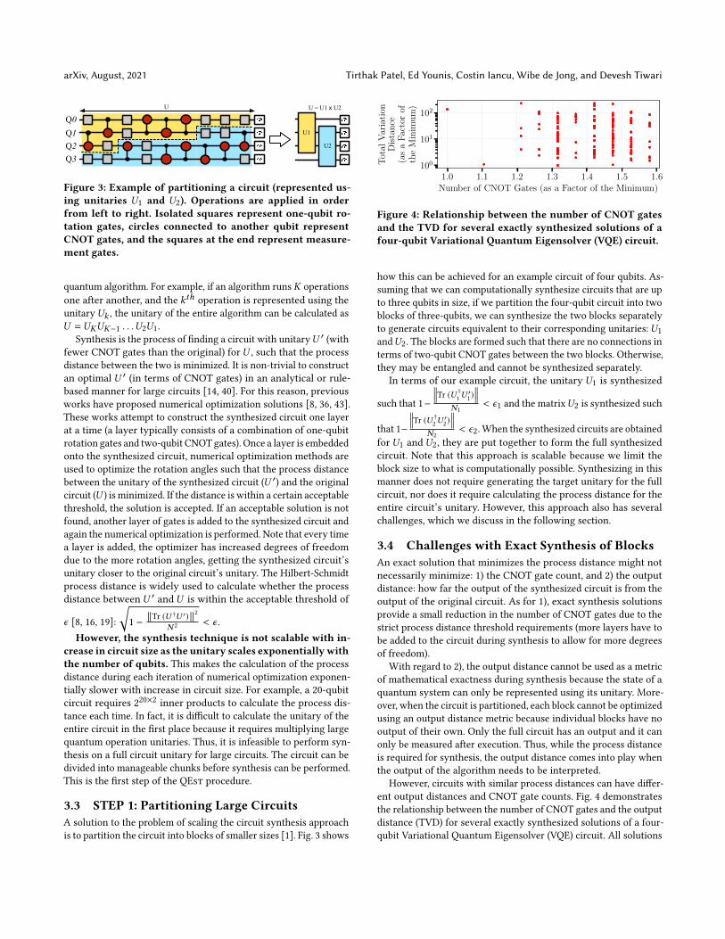
A solution to the problem of scaling the circuit synthesis approachis to partition the circuit into blocks of smaller sizes [1]. Fig. 3 shows

1.0 1.1 1.2 1.3 1.4 1.5 1.6Number of CNOT Gates (as a Factor of the Minimum)

100

101

102

Tot

alV

aria

tion

Dis

tan

ce(a

sa

Fac

tor

ofth

eM

inim

um

)

Figure 4: Relationship between the number of CNOT gates

and the TVD for several exactly synthesized solutions of a

four-qubit Variational Quantum Eigensolver (VQE) circuit.

how this can be achieved for an example circuit of four qubits. As-suming that we can computationally synthesize circuits that are upto three qubits in size, if we partition the four-qubit circuit into twoblocks of three-qubits, we can synthesize the two blocks separatelyto generate circuits equivalent to their corresponding unitaries: 𝑈1and𝑈2. The blocks are formed such that there are no connections interms of two-qubit CNOT gates between the two blocks. Otherwise,they may be entangled and cannot be synthesized separately.

In terms of our example circuit, the unitary 𝑈1 is synthesized

such that 1−

Tr (𝑈 †1𝑈 ′1) 𝑁1

< 𝜖1 and the matrix𝑈2 is synthesized such

that 1−

Tr (𝑈 †2𝑈 ′2) 𝑁2

< 𝜖2. When the synthesized circuits are obtainedfor 𝑈1 and 𝑈2, they are put together to form the full synthesizedcircuit. Note that this approach is scalable because we limit theblock size to what is computationally possible. Synthesizing in thismanner does not require generating the target unitary for the fullcircuit, nor does it require calculating the process distance for theentire circuit’s unitary. However, this approach also has severalchallenges, which we discuss in the following section.

3.4 Challenges with Exact Synthesis of Blocks

An exact solution that minimizes the process distance might notnecessarily minimize: 1) the CNOT gate count, and 2) the outputdistance: how far the output of the synthesized circuit is from theoutput of the original circuit. As for 1), exact synthesis solutionsprovide a small reduction in the number of CNOT gates due to thestrict process distance threshold requirements (more layers have tobe added to the circuit during synthesis to allow for more degreesof freedom).

With regard to 2), the output distance cannot be used as a metricof mathematical exactness during synthesis because the state of aquantum system can only be represented using its unitary. More-over, when the circuit is partitioned, each block cannot be optimizedusing an output distance metric because individual blocks have nooutput of their own. Only the full circuit has an output and it canonly be measured after execution. Thus, while the process distanceis required for synthesis, the output distance comes into play whenthe output of the algorithm needs to be interpreted.

However, circuits with similar process distances can have differ-ent output distances and CNOT gate counts. Fig. 4 demonstratesthe relationship between the number of CNOT gates and the outputdistance (TVD) for several exactly synthesized solutions of a four-qubit Variational Quantum Eigensolver (VQE) circuit. All solutions


Q0

Q1

Q2

Figure 5: Leap compiler builds the circuit layer-by-layer.

have a similar process distance of less than 10−5 (exact solutionthreshold) and yet have TVDs in a large range. The solution withthe minimum number of CNOT gates has one of the highest TVDs,while the solution with only 10% more CNOT gates than the mini-mum (1.1 factor) has a lower TVD. This small-scale example showsthat it is not always advisable to select the exact solution with thefewest number of CNOT gates. Thus, QEst breaks away from thenotion of having an exact synthesized solution by designing anapproximate synthesis approach.

3.5 STEP 2: Generate Approximate Circuits for

Blocks

QEst employs an approximate synthesis procedure that generatesmultiple low-CNOT-gate-count circuit approximations in a mannerthat minimizes the output distance between the synthesized circuitsand the original circuit of a block.

The key to achieving this reduction is realizing that differenttypes of circuits can be synthesized such that they have process dis-tance below a certain threshold. Recall that synthesis is performedusing numerical optimization building layer-by-layer. The qubitsthat these layers are placed on and the rotation angles that areassigned to them during the process distance minimization proce-dure affects the final synthesized circuit that is produced. Multipledifferent approximate circuits can be produced by varying thesefactors.

To achieve this, QEst modifies the Leap compiler [36] to returnthe best𝑀 circuits with the lowest process distance at each layer ofthe compiler tree. The compiler constructs a circuit tree one layerat a time as shown in Fig. 5. Each layer consists of a CNOT gatebetween two qubits followed by two rotation gates on both thequbits. It attempts this layer on all allowed two-qubit combinationsand optimizes the rotation angles to minimize the unitary processdistance. As more layers are added, the tree expands due to theincreased number of layer permutations. Every few layers, it picksthe branch with the least process distance and starts reconstructingthe tree from there to reduce the number of optimization evalua-tions. QEst uses the compiler to generate multiple approximationsat each layer of the tree (a tree layer roughly corresponds to oneCNOT gate). This enables the generation of approximate circuitsof different qualities in terms of process distances for each blockat different CNOT gate counts. All approximate solutions are gen-erated until the tree exceeds the CNOT gate count of the originalcircuit. As more layers are constructed and the tree becomes deeper,the process distance decreases. However, because we would like tohave multiple solutions for a block, including the ones with higherCNOT gate counts than the minimum CNOT gate count solution,we collect all solutions of different CNOT gate counts.

Process Distance Boundary

1 Sample 3 Samples 5 Samples

Target Output

Synthesis Samples

Average of Samples

Figure 6: Visual representation of how averaging over mul-

tiple approximations in the can produce a similar output as

the original circuit (with the average having a low output

distance).

3.6 STEP 3: Putting Together Approximate

Blocks

How can these low-CNOT-gate-count approximations be used toreduce the output distance? Fig. 6 demonstrates a visual example ofhow selecting multiple synthesized circuits can help ensure that theoutput distance is reduced. The figure is read from left to right, withthe first circle showing when one approximate circuit sample isused and the last circle showing when six samples are used. The redcross shows the output of the original circuit in Hilbert space, theboundary circle around it demarcates the boundary of the processdistance threshold used for approximate synthesis (this threshold islarger than used with exact synthesis so as to generate low-CNOT-gate-count solutions). The blue squares show the output samplesof the approximate synthesized circuit and the dark blue diamondshows the average of the samples. We make two points:

1) If only the circuit with the fewest number of CNOT gates isselected, it can result in a high output distance as shown in the firstcircle. While the circuit with the lowest CNOT gate count mightalso coincidentally have a low output distance for some algorithms,this cannot be established analytically as it assumes knowing theground truth output. Instead, averaging over 𝑀 low-CNOT-gate-count circuits can help us regulate and control the output distancewith more robustness than simply choosing one circuit. The trade-offhere is between the CNOT gate count and the output distance. Ifmultiple circuits are not selected, we do not have a way to controland reduce the output error. On the other hand, if the CNOT gatecount is high, it defeats the purpose of synthesis.

2) It is also not sound to just have many random approximations.If the approximations are mathematically similar (e.g., if the sixsamples in the third circle were in the same region of the circle),their output cannot average out to reduce the output distance. Thus,QEst must ensure that the approximations are “dissimilar,” whilealso having a low CNOT count.

QEst achieves this balance by using a dual-annealing-basedminimization algorithm [33] shown in Algorithm 1 to minimize anobjective function that places equal weight on CNOT-gate count andthe dissimilarity of the approximations:min 𝑓 = 1

2 ×CNOT Count+12 × Approx. DissimilarityThe CNOT count in this objective function is simply the nor-

malized CNOT gate count of the approximation compared to theoriginal circuit. The approximation dissimilarity is calculated as thefraction of already selected circuit samples with similarity to thenew sample. Consider two approximate circuit samples, 𝑆1 and 𝑆2.If the process distance between the two samples (⟨𝑆1, 𝑆2⟩𝐻𝑆 ) is less


Algorithm 1 Dual annealing engine’s objective function.1: 𝑂 ← Original circuit2: 𝐴← Approximate circuit to score3: 𝑆 ← Already selected approximations4: 𝑐𝑛𝑜𝑟𝑚 ← (CNOT count of 𝐴) / (CNOT count of 𝑂)5: 𝜖 ← Process distance threshold6: if ⟨𝐴,𝑂⟩𝐻𝑆 > 𝜖 then ⊲ If the threshold is breached7: return 1.08: else if 𝑆 == {∅} then ⊲ If this is the first sample9: return 𝑐𝑛𝑜𝑟𝑚10: else11: 𝑚 = 0 ⊲ Fraction of similar samples12: for 𝑠 ∈ 𝑆 do

13: 𝑚 =𝑚 + ⟨𝐴, 𝑠⟩𝐻𝑆 ≤ max{⟨𝐴,𝑂⟩𝐻𝑆 , ⟨𝑂, 𝑠⟩𝐻𝑆 }14: end for

15: 𝑚 =𝑚/size(𝑆)16: return

12 ×𝑚 +

12 × 𝑐𝑛𝑜𝑟𝑚

17: end if

than the maximum of their process distances to the original circuit(max{⟨𝑆1,𝑂⟩𝐻𝑆 , ⟨𝑂, 𝑆2⟩𝐻𝑆 }), then the two samples are consideredsimilar: ⟨𝑆1, 𝑆2⟩𝐻𝑆 ≤ max{⟨𝑆1,𝑂⟩𝐻𝑆 , ⟨𝑂, 𝑆2⟩𝐻𝑆 }. Intuitively, inthe visualization shown in Fig. 6, this means that both samples arein the same region of the circle. If the process distance betweenthe two is greater than the maximum of their process distancesto the original circuit, then the two circuits are on the oppositeside of the circuit; thus, their output can be averaged out. The firstsample has an approximation dissimilarity of zero (since there areno already selected circuits), and the objective function will selectthe approximate circuit with the lowest CNOT-gate count. As moresamples are selected, the approximation dissimilarity gains moresignificance as it becomes increasingly difficult to find dissimilar ap-proximations. However, the equal weight on CNOT count ensuresthat approximations that have too many CNOTs are not selected.

While this objective function works well for non-partitionedcircuits, it requires a tweak to accommodate large partitioned cir-cuits. Calculating if two full circuit approximations (constructed byputting together block approximations) are similar should not re-quire the computationally infeasible use of the full circuit unitaries.Instead, QEst uses the metric “fraction of all circuit blocks that aresimilar” in the objective function as it is a scalable alternative thatworks well in practice. As an instance, for two approximations of afull circuit consisting of ten blocks, if three of the blocks are mathe-matically similar, the two approximations receive a similarity scoreof 0.3. Next, we discuss a major challenge when approximatinglarge partitioned circuits.

3.7 A Challenge of Approximating Full

Circuits

While for individual blocks it can be ensured that the approxima-tions are not too coarse by eliminating ones with a high outputdistance (Lines 6-7 in Algorithm 1), a major challenge of partitionedsynthesis is to ensure that when the approximate blocks are putback together, the process distance of the full circuit approximationis not violated. Blocks cannot be combined without the knowledge

of how their process distances accumulate. For example, the pro-cess distance may compound multiplicatively when the blocks arecombined to form the full circuit. Without having a theoreticalbound on the process distance of the full circuit, the process dis-tance thresholds of its blocks may have to be kept unnecessarilysmall to be on the safe side. This means that the synthesized blockslikely end up being longer than they need to be as more layersare typically required during the numerical optimization process ifthe distance threshold is very small. Overcoming this problem canhelp us synthesize shorter circuits with fewer CNOT operations.To this end, next we provide a theoretical proof to bound the fullcircuit process distance based on the process distances of its blockswithout the need to directly calculate the process distance of the fullcircuit. This will help us ensure that the full circuit approximationsthat are too coarse can be eliminated during the dual annealingminimization procedure.

3.8 Theoretical Upper Bound on Process

Distance

We prove the theoretical upper bound for a circuit partitioned intotwo blocks without any loss of generality (e.g., the one shown inFig. 3), and it can then be extended to a circuit partitioned into 𝐾blocks.

We want the process distance of the unitary𝑈 of the full circuitto be bounded without performing synthesis on the full circuit due

to the lack of scalability:

√︂1 − ∥Tr (𝑈

†𝑈 ′)∥2𝑁 2 < 𝜖 . 𝑈 is an 𝑁 × 𝑁

matrix, where 𝑁 is 2𝑛 , where 𝑛 is the number of qubits in the

full circuit. We choose the

√︂1 − ∥Tr (𝑈

†𝑈 ′)∥2𝑁 2 metric for process

distance as it is a reasonable metric to measure unitary equivalency,it is computationally efficient, and it gives us the ability to provea bound on it without calculating it directly. The 𝜖 bound needsto be derived based on the process distances of its circuit blocks.Recall that the partitioned blocks are small enough to be efficientlysynthesizable and therefore, have known process distances. Theexample circuit has two blocks and these blocks have the below twoprocess distance bounds by construction (synthesis is performed ina manner that ensures that these bounds are met).√√√√√

1 −

Tr (𝑈 †1𝑈 ′1) 2𝑁 21

≤ 𝜖1 ,

√√√√√1 −

Tr (𝑈 †2𝑈 ′2) 2𝑁 22

≤ 𝜖2 (1)

Here, 𝑁1 and 𝑁2 are the dimensions of𝑈1 and 𝑈2, respectively.For the example circuit, we have 𝑈 = (𝐼 ⊗ 𝑈2) (𝑈1 ⊗ 𝐼 ) = 𝑈𝐼2𝑈1𝐼 .The notation 𝑈1𝐼 refers to the unitary (𝑈1 ⊗ 𝐼 ), representing theKronecker product of the 𝑈1 operation with the identity operationon the remaining qubits (no operation can be represented as theidentity operation). Similarly,𝑈𝐼2 refers to the unitary (𝐼 ⊗𝑈2). Thepost-synthesis approximations of these unitaries can be representedas𝑈 ′ = (𝐼 ⊗ 𝑈 ′2) (𝑈

′1 ⊗ 𝐼 ) = 𝑈

′𝐼2𝑈′1𝐼 . Also, 𝑁 = 𝑁𝐼 × 𝑁1 = 𝑁2 × 𝑁𝐼 .

As a first step, we prove the process distance bound when a uni-tary representing a partitioned block is extended to the remainingqubits in the full circuit, i.e., we determine the process distance of𝑈1 ⊗ 𝐼 matrix given the process distance of the𝑈1 matrix. We begin


by rearranging the terms in Eq. 1 to isolate for Tr (𝑈 †1𝑈 ′1) , as is

shown below.

√√√√√1 −

Tr (𝑈 †1𝑈 ′1) 2𝑁 21

≤ 𝜖1 ⇒

Tr (𝑈 †1𝑈 ′1) 2𝑁 21

≥ 1 − 𝜖21

⇒ Tr (𝑈 †1𝑈 ′1) 2 ≥ 𝑁 2

1 (1 − 𝜖21 ) ⇒

Tr (𝑈 †1𝑈 ′1) ≥ 𝑁1

√︃1 − 𝜖21

(2)

Next, we show how Tr (𝑈 †1𝐼𝑈′1𝐼 ) is related to Tr (𝑈 †1𝑈

′1):

Tr (𝑈 †1𝐼𝑈′1𝐼 ) = Tr [(𝑈1 ⊗ 𝐼 )† (𝑈 ′1 ⊗ 𝐼 )] = Tr [(𝑈 †1 ⊗ 𝐼

†) (𝑈 ′1 ⊗ 𝐼 )]

= Tr [(𝑈 †1 ⊗ 𝐼 ) (𝑈′1 ⊗ 𝐼 )] = Tr (𝑈 †1𝑈

′1 ⊗ 𝐼 𝐼 ) = Tr (𝑈 †1𝑈

′1 ⊗ 𝐼 )

= Tr (𝑈 †1𝑈′1)tr(I) = Tr (𝑈 †1𝑈

′1)𝑁𝐼

(3)

Substituting Eq. 2 into Eq. 3, we get that Tr (𝑈 †1𝐼𝑈 ′1𝐼 ) ≥ 𝑁√︃

1 − 𝜖21 ,as shown below. Tr (𝑈 †1𝐼𝑈 ′1𝐼 ) = Tr ((𝑈 †1𝑈 ′1)𝑁𝐼 = Tr ((𝑈 †1𝑈 ′1) 𝑁𝐼

≥ 𝑁1

√︃1 − 𝜖21𝑁𝐼 = 𝑁1𝑁𝐼

√︃1 − 𝜖21 = 𝑁

√︃1 − 𝜖21

(4)

If we rearrange the terms in Eq. 4 (similar to the rearranging in

Eq. 2, but in reverse order), we get

√︄1 −

Tr (𝑈 †1𝐼𝑈 ′1𝐼 ) 2𝑁 2 ≤ 𝜖1. Thus,

the process distance of a block unitary that does not span the fullsize (number of qubits) of a circuit remains bounded by the samethreshold when the unitary is extended to the size of the circuit.Therefore, using a similar procedure, we can also show that for the

second block,𝑈2,

√︄1 −

Tr (𝑈 †𝐼2𝑈 ′𝐼2) 2𝑁 2 ≤ 𝜖2.

We now have the tools to bound the process distance of thefull circuit. Recall that the process distance for the full circuit is√︂1 − ∥Tr (𝑈

†𝑈 ′)∥2𝑁 2 . Substituting 𝑈 = 𝑈𝐼2𝑈1𝐼 , we obtain the follow-

ing: √︄1 −

Tr (𝑈 †𝑈 ′) 2𝑁 2 =

√︄1 −

Tr [(𝑈𝐼2𝑈1𝐼 )† (𝑈 ′𝐼2𝑈′1𝐼 )]

2𝑁 2

=

√√√1 −

Tr (𝑈 †1𝐼𝑈 †𝐼2𝑈 ′𝐼2𝑈 ′1𝐼 ) 2𝑁 2 =

√√√1 −

Tr [(𝑈 ′1𝐼𝑈 †1𝐼 ) (𝑈 †𝐼2𝑈 ′𝐼2)] 2𝑁 2

(5)

Using the inequality proven by Wang and Zhang [41] and usingthe above derived bounds for process distances of 𝑈1𝐼 and𝑈𝐼2, thefollowing relationship is obtained:√√√

1 −

Tr [(𝑈 ′1𝐼𝑈 †1𝐼 ) (𝑈 †𝐼2𝑈 ′𝐼2)] 2𝑁 2

≤

√√√1 −

Tr (𝑈 ′1𝐼𝑈 †1𝐼 ) 2𝑁 2 +

√√√1 −

Tr (𝑈 †2𝐼𝑈 ′2𝐼 ) 2𝑁 2

≤

√√√1 −

Tr (𝑈 †1𝐼𝑈 ′1𝐼 ) 2𝑁 2 +

√√√1 −

Tr (𝑈 †2𝐼𝑈 ′2𝐼 ) 2𝑁 2

≤ 𝜖1 + 𝜖2

(6)

10−8 10−6 10−4 10−2 100

Process Distance Upper Bound

10−8

10−5

10−2

101

Pro

cess

Dis

tan

ce

Figure 7: The theoretical process distance upper bound suc-

cessfully bounds the process distance in practice.

Combining Eq. 5 and Eq. 6, we get

√︂1 − ∥Tr (𝑈

†𝑈 ′)∥2𝑁 2 ≤ 𝜖1 + 𝜖2.

This proof can be extended to circuits partitioned into 𝐾 blocksby providing the proof for two blocks at a time, combining thetwo into a single unitary and providing the proof again for the twounitaries (combined unitary and the third unitary), and so on and soforth, iteratively. Therefore, for a circuit partitioned into 𝐾 blocks, we

have that

√︂1 − ∥Tr (𝑈

†𝑈 ′)∥2𝑁 2 ≤

𝑘=𝐾∑︁𝑘=1

𝜖𝑘 . The process distance of the

full circuit is theoretically upper bounded by the sum of the processdistances of all of its partitioned blocks.

While the relationship between the derived process distance up-per bound and the actual process distance cannot be directly/theoreticallyproven as it algorithm specific and varies depending on how thealgorithm circuit is constructed and partitioned, we demonstratethis relationship using real algorithm examples. Fig. 7 shows the re-lationship between the process distance upper bound and the actualprocess distance for different algorithms. The results indicate thatthe derived upper bound is respected across all samples and a rela-tively tight bound is obtained for different algorithms and processdistance values. Therefore, the upper bound enables us to confi-dently bound the process distance of the full circuit (without theneed to calculate it directly) simply by ensuring that its partitionedblocks are combined by the dual annealing engine in a manner thatthe sum of their process distances is within an acceptable threshold.

Putting it togerher. In summary, QEst enables reduction in theCNOT gate count by partitioning the circuit into smaller blocks andgenerating multiple approximate circuits for the blocks. It then putsback together the block approximations in a manner that reducesthe CNOT gate count as well as generates dissimilar approxima-tions to reduce the output distance using its dual annealing engine.It is aided by the theoretical upper bound to eliminate coarse ap-proximations in a scalable manner. In the next section, we evaluatethe effectiveness of QEst for different algorithms after providingdetails about the experimental setup and methodology.

4 EVALUATION

4.1 Experimental Setup and Methodology

Comparative Techniques.We compare against the original cir-cuit as a baseline circuit (referred to as the Baseline) in terms ofthe CNOT gate count, ground truth output, as well as the errorobserved in a noisy environment. We also compare to the circuitgenerated when all the Qiskit compiler optimizations are appliedto this Baseline circuit. These compiler optimizations are simply


Table 1: Algorithms and benchmarks used to evaluateQEst.

Algorithm Description

Adder Quantum adder circuit [7]Heisenberg Time-independent Heisenberg Hamiltonian [3]HLF Hidden linear function [4]QFT Quantum Fourier transform [28]QAOA Quantum alternating operator ansatz [10]Multiplier Quantum multiplier circuit [12]TFIM Transverse field ising model [3]VQE Variational quantum eigensolver [24]XY XY quantum Heisenberg model [3]

referred to as Qiskit. When these compiler passes are applied tothe approximate circuits produced by QEst, the results generatedby the produced circuits are referred to as QEst + Qiskit.

Experimental Setup. The partitioning, approximate synthesis,and dual annealing components of QEst are run on our local com-pute cluster consisting of 2.4 GHz Intel E5-2680 v4 CPUs. A maxi-mum block size of four qubits is used to partition the circuits usingthe scan partitioner available as part of the open-source BQSKitpackage [1]. It forms partitions by traversing the circuit left to rightand creating four-qubit blocks. Note that some blocks may be ofa smaller size if need be. A maximum block size of four qubits isused as it synthesizes efficiently and yields good results. When analgorithm has multiple blocks, the approximate synthesis step isrun on different blocks in parallel on up to ten compute nodes. Leapcompiler [36], which is also a part of the BQSKit package, is modi-fied and used for synthesis as described in Sec. 3. The Python-basedSciPy package is used to run the dual annealing engine [15]. Theprocess distance threshold to eliminate coarse approximations inthe annealing engine is set proportional to the number of blocks inthe circuit and up to 16 approximations are generated for each al-gorithm. A balanced weight of 0.5 is used for CNOT gate count andapproximation dissimilarity in the objective function that the dualannealing engine minimizes. The ground truth results are obtainedby running the Baseline circuit in an ideal quantum simulationenvironment using the Qiskit unitary simulator [25], which is partof the Aer package. We perform noisy simulations on circuits upto 16 qubits (it was not possible to run noisy simulations on largercircuits) using the IBMQ QASM simulator available via the IBMquantum experience cloud. A Pauli noise model is used for all thequbits with noise levels of 1%, 0.5%, and 0.1% to simulate how QEstwill perform for future NISQ computers as the noise level decreases.We run circuits up to five qubits on the IBMQ Manila quantumcomputer in order to demonstrate how the technique performson existing quantum computers. We use 8192 experimental trials(maximum allowed) per experiment. Each circuit run on a quantumcomputer takes 10-12 seconds for all trials.

Algorithms and Benchmarks.We use the algorithms and bench-marks listed in Table 1 to evaluate QEst. Adder and Multiplierare standard quantum arithmetic circuits, while QAOA and VQEare quantum variational algorithms. Heisenberg, TFIM, and XYare time-evolving Hamiltonian algorithms for material simulations.

Ad

der

4

Ad

der

9

Hei

sen

.4

Hei

sen

.8

HL

F5

HL

F10

QF

T5

QF

T10

QA

OA

5

QA

OA

10

Mu

ltip

ly5

Mu

ltip

ly10

TF

IM4

TF

IM8

TF

IM16

TF

IM32

VQ

E4

XY

4

XY

8

0

25

50

75

100

Imp

rove

men

tin

Nu

mb

erof

CN

OT

Gat

es(%

)

Qiskit Quest Quest + Qiskit

Figure 8: QEst reduces the CNOT gate count across all algo-

rithms compared to theBaseline circuits aswell as theQiskit

optimizations applied on the Baseline circuits. The number

next to the algorithm name indicates the number of qubits.

The Heisenberg model has non-zero strength for the coupling in-teraction between nearest neighbor spins for all three axes (𝑥,𝑦, 𝑧),TFIM does for 𝑧, and XY does for 𝑥 and 𝑦. We evaluate circuits ofsize 4-32 qubits.

Evaluation Metrics. In terms of output distance, we use the To-tal Variation Distance (TVD) and the Jensen-Shannon Divergence(JSD) as defined in Sec. 2. These are general metrics that are typi-cally used to define the output distance across all algorithms. Tocalculate the output distance from the Baseline for QEst, the out-put probability distributions of all of its approximate circuits areaveraged to generate one probability distribution. In addition tothese metrics, we also study algorithm-specific output distances asnecessary. For example, for TFIM and Heisenberg algorithms, westudy the differences in the magnetization at different time steps.

4.2 Results and Analysis

QEst considerably reduces the CNOT gate count over the Baselinecircuit compared to the Qiskit compiler optimizations. Fig. 8 shows thepercent improvement, i.e., reduction, in CNOT gate count over theBaseline circuit with Qiskit, QEst and QEst + Qiskit for differentalgorithms. QEst delivers a reduction in CNOT gate count of 30-80% for most algorithms, even greater than 80% for some algorithmssuch as Heisenberg, which has many CNOT gates. In comparison,the Qiskit compiler optimizations can prove to be less effectivedepending on the algorithm. For the Heisenberg circuit, Qiskitgives over a 30% reduction in the CNOT gate count. But for mostother circuits the reduction is negligible, even resulting in a slightincrease in the CNOT gate count for some algorithms such as HLFand Multiply. In contrast, QEst always performs better than Qiskitand never performs worse than the Baseline.

When the Qiskit compiler optimizations are added on top ofthe approximate circuits produced by QEst, there can be a slightimprovement or degradation in CNOT count depending on thealgorithm. For example, QEst + Qiskit performs better than QEstfor the eight-qubit Heisenberg circuit, but it performs worse for thefour-qubit XY circuit. Nonetheless, for most algorithms we observethat it does not diminish the gains of QEst and so we use the QEst+ Qiskit configuration for evaluation results going forward.


Ad

der

4

Ad

der

9

Hei

sen

.4

Hei

sen

.8

HL

F5

HL

F10

QF

T5

QF

T10

QA

OA

5

QA

OA

10

Mu

ltip

ly5

Mu

ltip

ly10

TF

IM4

TF

IM8

TF

IM16

TF

IM32

VQ

E4

XY

4

XY

8

0.0

0.5

1.0

Tot

alV

aria

tion

Dis

tan

ce

1e-1

4

1e-1

4

2e-0

3

2e-0

7

1e-0

2

6e-0

3

1e-0

3

6e-0

2

5e-0

8

8e-0

8

9e-1

6

7e-0

8

5e-0

3

2e-0

2

7e-0

3

2e-0

2

2e-0

2

2e-0

4

2e-1

0

(a) Total Variation Distance

Ad

der

4

Ad

der

9

Hei

sen

.4

Hei

sen

.8

HL

F5

HL

F10

QF

T5

QF

T10

QA

OA

5

QA

OA

10

Mu

ltip

ly5

Mu

ltip

ly10

TF

IM4

TF

IM8

TF

IM16

TF

IM32

VQ

E4

XY

4

XY

8

0.0

0.5

1.0

Jen

sen

-Sh

ann

onD

iver

gen

ce

7e-0

8

6e-0

8

1e-0

2

1e-0

6

1e-0

2

5e-0

3

1e-0

3

5e-0

2

5e-0

8

7e-0

8

2e-0

8

1e-0

7

2e-0

2

5e-0

2

3e-0

2

7e-0

2

1e-0

2

9e-0

3

9e-0

6(b) Jensen-Shannon Divergence

Figure 9: QEst ensures low output distance from the ideal

output while delivering a reduction in CNOT gate count.

Add

er4

Heis

en. 4

HLF

5

QFT

5

QAO

A5

Mul

tiply

5

TFIM4

VQE

4

XY

40.00.20.40.60.81.0

Tot

alV

aria

tion

Dis

tan

ce

Qiskit Quest + Qiskit

Figure 10:QEst +Qiskit reduces the TVD compared toQiskit

when the circuits are run on the IBMQ Manila computer.

QEst’s approximations result in a low output distance even in the idealquantum computing scenario.We now evaluate if the approximatecircuits produced by QEst are resulting in the correct output (closeto ground truth results) even in the absence of noise. This can helpus understand if the approximate circuits are closely emulating theexpected output of the Baseline circuit. Fig. 9(a) and (b) show theTVD and JSD, respectively, between the ground truth output of theBaseline circuit and the approximated noiseless output of QEst.The figure shows that both the output distance metrics have lowvalues across all algorithms. Given the corresponding reductionin CNOT gate count, these results signify the usefulness of circuitapproximations even in a fault-tolerant environment. As both met-rics have similar trends, we use only the TVD going forward forbrevity.

QEst delivers a significant reduction in TVD on a real NISQ machine.Next, we evaluate the performance of QEst on IBMQ Manila, oneof the most recent and least error quantum computers availablevia IBMQ open access for algorithms which were possible to run.Fig. 10 shows the TVD from the ground truth when the algorithmsare run with just the Qiskit optimizations vs. when they are run

with QEst + Qiskit. While the raw TVD numbers are large for mostalgorithms due to the high noise of the current state-of-the-artquantum computers, QEst + Qiskit reduces the TVD by over 0.3or 30% points in some cases. For example, for the four-qubit TFIMcircuit, the TVD drops from 0.35 to 0.08.

QEst delivers a significant reduction in TVD even for larger circuitsand as hardware noise is decreased in a quantum simulation. Wenow present larger circuits run in a noisy simulation environmentwith noise levels of 1%, 0.5%, and 1% in Fig. 11(a), (b), and (c), re-spectively. The figures show the percentage reduction in TVD com-pared to when the Baseline circuit is run with a noisy simulationfor Qiskit and QEst + Qiskit. We see that across the board, QEst+ Qiskit reduces the TVD even as the hardware noise is reduced.This demonstrates the usefulness of circuit approximations evenwhen projected on to the future when the noise is reduced by 10×(0.1% compared to the current average noise of over 1%).QEst incurs one-time cost for building approximate circuits to yieldmeaningful output quality for circuits with a large number of CNOTgates. QEst’s approximate circuit building process consists of threesteps: (1) partitioning, (2) synthesis, and (3) dual-annealing engine.Fig. 12(a) and (b) show absolute time required for different circuitand relative contribution from each step. Overall, for most circuitsQEst can be completed within a few hours. The only exception isTFIM 32 which takes almost a full day. Partitioning takes up most ofthe time due to TFIM circuit structure. Synthesis and dual-annealingengines are not major contributers.

While this one-time cost is non-negligible, it has potential forsignificant reduction (e.g., all blocks can be synthesized in parallel).But, we did not need to focus on reducing this overhead because ofthe feedback provided by the domain scientists and physicists whoare actively working and improving the two major target applica-tions. They assessed this cost is hidden in the code developmentand improvement cycle, and hence, wanted this effort to focus onobtaining meaningful output quality. For example, the magnetiza-tion curve for the Heisenberg application should match the groundtruth curve. QEst achieved these algorithmic and science goals, asconfirmed by our case study on TFIM and Heisenberg over theirentire time evolution landscape (discussed below).

Also, we note that this overhead is not incurred each time theprogram needs to be compiled with Qiskit and executed. This isbecauseQEst produces full approximate circuits as one-time output.This one-time output can be compiled with Qiskit (in the order ofseconds) whenever needed for optimally mapping the approximatecircuit on physical qubits.

4.3 TFIM and Heisenberg: A Case Study

QEst +Qiskit is able tomore closely track the ground truth output thanjust Qiskit optimizations due to the larger reduction in the number ofCNOT gates. Fig. 13 shows the time evolutions of the four-spin TFIMand Heisenberg circuits with ground truth, and the Qiskit circuit,and QEst + Qiskit approximate circuits when run on the IBMQManila computer. Each step in the time evolution is a differentcircuit that is separately run with QEst. For the TFIM algorithm,the QEst + Qiskit magnetization line is more stable and closer inmagnitude to the ground truth than is the Qiskit magnetization


Ad

der

4A

dd

er9

Hei

sen

.4

Hei

sen

.8

HL

F5

HL

F10

QF

T5

QF

T10

QA

OA

5Q

AO

A10

Mu

ltip

ly5

Mu

ltip

ly10

TF

IM4

TF

IM8

TF

IM16

VQ

E4

XY

4X

Y8

0

50

Imp

rove

men

tin

Tot

alV

aria

tion

Dis

tan

ce(%

)


(a) 1% Noise

Ad

der

4A

dd

er9

Hei

sen

.4

Hei

sen

.8

HL

F5

HL

F10

QF

T5

QF

T10

QA

OA

5Q

AO

A10

Mu

ltip

ly5

Mu

ltip

ly10

TF

IM4

TF

IM8

TF

IM16

VQ

E4

XY

4X

Y8

0

50

Imp

rove

men

tin

Tot

alV

aria

tion

Dis

tan

ce(%

)


(b) 0.5% Noise

Ad

der

4A

dd

er9

Hei

sen

.4

Hei

sen

.8

HL

F5

HL

F10

QF

T5

QF

T10

QA

OA

5Q

AO

A10

Mu

ltip

ly5

Mu

ltip

ly10

TF

IM4

TF

IM8

TF

IM16

VQ

E4

XY

4X

Y8

0

50

100

Imp

rove

men

tin

Tot

alV

aria

tion

Dis

tan

ce(%

)


(c) 0.1% Noise

Figure 11: Noisy simulations with different levels of noise indicate that QEst can reduce TVD even for future NISQ devices.

Ad

der

4

Ad

der

9

Hei

sen

.4

Hei

sen

.8

HL

F5

HL

F10

QF

T5

QF

T10

QA

OA

5

QA

OA

10

Mu

ltip

ly5

Mu

ltip

ly10

TF

IM4

TF

IM8

TF

IM16

TF

IM32

VQ

E4

XY

4

XY

8

104

Exec

uti

onT

ime

(s)

(a) Execution Times

Ad

der

4

Ad

der

9

Hei

sen

.4

Hei

sen

.8

HL

F5

HL

F10

QF

T5

QF

T10

QA

OA

5

QA

OA

10

Mu

ltip

ly5

Mu

ltip

ly10

TF

IM4

TF

IM8

TF

IM16

TF

IM32

VQ

E4

XY

4

XY

8

0

50

100

Exec

uti

onT

ime

(%)

Partitioning Synthesis Dual Annealing

(b) Execution Time Division

Figure 12: The execution time overhead of QEst and its di-

vision among the different steps varies for different algo-

rithms.

10 20 30 40 50 60 70 80 90 100Timestep

0.8

0.9

1.0

Ave

rage

Mag

net

izat

ion

Ground Truth

Quest + Qiskit

Qiskit

(a) TFIM 4

5 10 15 20 25 30 35 40 45 50Timestep

−0.5

0.0

0.5

Sta

gger

edM

agn

etiz

atio

n

Ground Truth

Quest + Qiskit

Qiskit

(b) Heisenberg 4

Figure 13: QEst achieves closer to the ground truth output

on the IBMQ Manila machine than the Baseline.

line. For Heisenberg, QEst very closely tracks the ground truthmagnetization, while Qiskit produces meaningless results.

In fact, Fig. 14 plots the simulation results with noise levels 1%,0.5%, and 0.1%, and the figure shows that projected reduction inhardware errors can further reduce the output distance for TFIM

10 20 30 40 50 60 70 80 90 100Timestep

0.8

0.9

1.0

Ave

rage

Mag

net

izat

ion

Ground Truth

1% Noise

.5% Noise

.1% Noise

(a) TFIM 4

5 10 15 20 25 30 35 40 45 50Timestep

−0.5

0.0

0.5

Sta

gger

edM

agn

etiz

atio

n

Ground Truth

1% Noise

.5% Noise

.1% Noise

(b) Heisenberg 4

Figure 14: For TFIM, QEst performs better as the hardware

noise decreases. For Heisenberg, QEst’s output is close to

ground truth even in a high noise environment of 1%.

Q0

Q1

Q2

Q3

Q0

Q1

Q2

Q3

Baseline: 12 CNOTs QUEST: 6 CNOTs

(a) TFIM 4

Q0

Q1

Q2

Q3

Q0

Q1

Q2

Q3

Baseline: 900 CNOTs QUEST: 11 CNOTs

(b) Heisenberg 4

Figure 15: Illustration of the reduction in the CNOT gate

count for one of the TFIM and Heisenberg approximate cir-

cuits.

and Heisenberg. This is due to the large reduction in the CNOTgate count of both the algorithms.

Fig. 15(a) shows that circuit structure of the TFIM algorithm atthe 100𝑡ℎ timestep with Baseline and one of the approximationsgenerated using QEst. Similarly, Fig. 15(b) shows the circuit struc-ture of the Heisenberg algorithm at the 50𝑡ℎ timestep. The figuresillustrate the large reduction in CNOT gate count. For example, forthe Heisenberg algorithm, the gate count reduced from 900 CNOTsto just 11 CNOTs with approximate circuits. This reduction enablesfewer operations errors and lower decoherence errors due to fasterexecution.


10 20 30 40 50 60 70 80 90 100Timestep

0.7

0.8

0.9

1.0

Ave

rage

Mag

net

izat

ion

Ground Truth

ε = 10−1

ε = 2e10−1

ε = 4e10−1

(a) TFIM 4

5 10 15 20 25 30 35 40 45 50Timestep

−0.5

0.0

0.5

Sta

gger

edM

agn

etiz

atio

n

Ground Truth

ε = 10−1

ε = 2e10−1

ε = 4e10−1

(b) Heisenberg 4

Figure 16: Careful selection of process distance threshold for

the dual annealing engine produces good approximations of

the TFIM and Heisenberg circuits.

QEst’s design decisions of using process distance upper bound thresh-old and dissimilar approximations yields good results. Fig. 16(a) and(b) shows the output of TFIM and Heisenberg algorithms for differ-ent process distance thresholds. Recall that if the threshold is settoo high, the dual annealing engine is likely to select coarse approx-imations selecting more circuits with fewer CNOT gate count thanselecting ones with dissimilar characteristics (approximations withlow process distances among them). The figures shows that thiscan lead to a large error in the output distance for both algorithms.Thus, careful selection of the threshold is required to ensure benefi-cial results. However, it also does not have to be tuned exhaustivelybecause as the figure shows, QEst performs well for a wide rangeof values. Therefore, we set the threshold to be proportional tothe number of blocks in the circuit and it works well across allalgorithms in practice.

5 RELATEDWORK

Quantum Circuit Compiling and Mapping. There has been alarge focus on attempting to leverage compiler-based passes andquantum computing rules to reduce CNOT and SWAP gate countsand perform noise- and layout- aware mapping of the qubits to thehardware [21, 26, 27, 35, 37, 39, 42, 44, 45].

For example, in the circuit mapping space, previous efforts haveexploited the diverse error characteristics of different qubits to mapthe same baseline circuit in different ways expecting the outputdistances to reduce [31, 38]. But these works do not target reducingthe CNOT count considerably by employing approximate synthesisto systematically generate dissimilar circuits and thus, have largeoutput distances.

Quantum Circuit Synthesis. QEst employs synthesis as one ofthe steps in its procedure to generate approximate circuits. Previoussynthesis works have attempted to synthesize circuits with onlyspecific gates (e.g., only CNOTs) or universal circuits as exactly aspossible with as few CNOT gates as possible [8, 13, 14, 17, 23, 29,34, 36, 43]. We use a modified version of the Leap synthesis tool forQEst as it performs better than previous approaches [36].

Despite the potential of approximations, not many proceduresto generate resource efficient approximations using synthesis haveexisted before QEst. Madden et al. [22] describe generative proce-dures using synthesis, but these procedures are non-scalable and

lack any apriori criteria for selecting approximations across dif-ferent algorithms. Amy et al. [2] describe a more scalable directsynthesis algorithm, but the approach leads to very long circuits,sometimes by orders of magnitude compared to other synthesistools. In comparison, QEst defines a clear criterion for selectingdissimilar approximate circuits apriori, provides a theoretical proofto bound process distance, and generates circuits with few CNOTs.

6 CONCLUSION

In this work, we present QEst, a technique to reduce CNOT gatecount of quantum circuits using approximate synthesis and distance-based approximation selection.We provided a theoretical derivationto bound the process distance of approximations as well as a dissim-ilarity criterion to select approximations in a manner that reducesthe output distance. QEst achieves a CNOT gate reduction of 30-80% across algorithms while maintaining a low output distancefrom the output of the original circuit. While QEst’s contributionsare beneficial in the NISQ era for minimizing the impact of noise,they are also useful for fault-tolerant quantum computers.

7 ACKNOWLEDGEMENTS

This work was supported by the Office of Science, Office of Ad-vanced Scientific Computing Research Accelerated Research forQuantum Computing Program of the U.S. Department of Energyunder Contract No. DE-AC02-05CH11231. This work was also sup-ported by Northeastern University, NSF Award 1910601, and theMassachusetts Green High Performance Computing Center (MGH-PCC) facility. This research used resources of the Oak Ridge Lead-ership Computing Facility, which is a DOE Office of Science UserFacility supported under Contract No. DE-AC05-00OR22725. IBMQ was also used for this work. The views expressed are those ofthe authors and do not reflect the official policy or position of IBMor the IBM Q team.

REFERENCES

[1] https://github.com/BQSKit. BQSKit: Berkeley Quantum Synthesis Toolkit.[2] Matthew Amy, Dmitri Maslov, Michele Mosca, and Martin Roetteler. 2013. A

Meet-in-the-Middle Algorithm for Fast Synthesis of Depth-Optimal QuantumCircuits. IEEE Transactions on Computer-Aided Design of Integrated Circuits andSystems 32, 6 (2013), 818–830.

[3] Lindsay Bassman, Connor Powers, and Wibe A de Jong. 2021. ArQTiC: A Full-Stack Software Package for Simulating Materials on Quantum Computers. arXivpreprint arXiv:2106.04749 (2021).

[4] Sergey Bravyi, David Gosset, and Robert König. 2018. Quantum Advantage withShallow Circuits. Science 362, 6412 (2018), 308–311.

[5] Heinz-Peter Breuer, Elsi-Mari Laine, and Jyrki Piilo. 2009. Measure for the Degreeof Non-Markovian Behavior of Quantum Processes in Open Systems. Physicalreview letters 103, 21 (2009), 210401.

[6] Davide Castelvecchi. 2017. IBM’s Quantum Cloud Computer Goes Commercial.Nature News 543, 7644 (2017), 159.

[7] Steven A Cuccaro, Thomas G Draper, Samuel A Kutin, and David Petrie Moulton.2004. A New Quantum Ripple-Carry Addition Circuit. arXiv preprint quant-ph/0410184 (2004).

[8] Marc G Davis, Ethan Smith, Ana Tudor, Koushik Sen, Irfan Siddiqi, and CostinIancu. 2020. Towards Optimal Topology Aware Quantum Circuit Synthesis. In2020 IEEE International Conference on Quantum Computing and Engineering (QCE).IEEE, 223–234.

[9] David Elieser Deutsch. 1989. Quantum Computational Networks. Proceedingsof the Royal Society of London. A. Mathematical and Physical Sciences 425, 1868(1989), 73–90.

[10] Edward Farhi and Aram W Harrow. 2016. Quantum Supremacy through theQuantum Approximate Optimization Algorithm. arXiv preprint arXiv:1602.07674(2016).


[11] Alexei Gilchrist, Nathan K Langford, and Michael A Nielsen. 2005. DistanceMeasures to Compare Real and Ideal Quantum Processes. Physical Review A 71,6 (2005), 062310.

[12] Andrew Hancock, Austin Garcia, Jacob Shedenhelm, Jordan Cowen, and CalistaCarey. 2019. Cirq: A Python Framework for Creating, Editing, and InvokingQuantum Circuits. URL https://github.com/quantumlib/Cirq (2019).

[13] Raban Iten, Roger Colbeck, Ivan Kukuljan, Jonathan Home, and Matthias Chri-standl. 2016. Quantum Circuits for Isometries. Physical Review A 93, 3 (2016),032318.

[14] Raban Iten, Oliver Reardon-Smith, Emanuel Malvetti, Luca Mondada, GabriellePauvert, Ethan Redmond, Ravjot Singh Kohli, and Roger Colbeck. 2019. Intro-duction to UniversalQCompiler. arXiv preprint arXiv:1904.01072 (2019).

[15] Eric Jones, Travis Oliphant, Pearu Peterson, et al. 2016. SciPy: Open SourceScientific Tools for Python, 2001.

[16] Sumeet Khatri, Ryan LaRose, Alexander Poremba, Lukasz Cincio, Andrew TSornborger, and Patrick J Coles. 2019. Quantum-Assisted Quantum Compiling.Quantum 3 (2019), 140.

[17] Aleks Kissinger and Arianne Meijer-van de Griend. 2019. CNOT Circuit Ex-traction for Topologically-Constrained Quantum Memories. arXiv preprintarXiv:1904.00633 (2019).

[18] Alexei Yu Kitaev, Alexander Shen, Mikhail N Vyalyi, and Mikhail N Vyalyi. 2002.Classical and Quantum Computation. Number 47. American Mathematical Soc.

[19] Vadym Kliuchnikov, Alex Bocharov, and Krysta M Svore. 2014. AsymptoticallyOptimal Topological Quantum Compiling. Physical review letters 112, 14 (2014),140504.

[20] Ang Li and SriramKrishnamoorthy. 2020. QASMBench: A Low-Level qasmBench-mark Suite for NISQ Evaluation and Simulation. arXiv preprint arXiv:2005.13018(2020).

[21] Gushu Li, Yufei Ding, and Yuan Xie. 2019. Tackling the Qubit Mapping Problemfor NISQ-Era Quantum Devices. In Proceedings of the Twenty-Fourth InternationalConference on Architectural Support for Programming Languages and OperatingSystems. ACM, 1001–1014.

[22] Liam Madden and Andrea Simonetto. 2021. Best Approximate Quantum Compil-ing Problems. arXiv preprint arXiv:2106.05649 (2021).

[23] Esteban A Martinez, Thomas Monz, Daniel Nigg, Philipp Schindler, and RainerBlatt. 2016. Compiling Quantum Algorithms for Architectures with Multi-QubitGates. New Journal of Physics 18, 6 (2016), 063029.

[24] Jarrod R McClean, Jonathan Romero, Ryan Babbush, and Alán Aspuru-Guzik.2016. The Theory of Variational Hybrid Quantum-Classical Algorithms. NewJournal of Physics 18, 2 (2016), 023023.

[25] David C McKay, Thomas Alexander, Luciano Bello, Michael J Biercuk, Lev Bishop,Jiayin Chen, Jerry M Chow, Antonio D Córcoles, Daniel Egger, Stefan Filipp, et al.2018. Qiskit Backend Specifications for OpenQASM and OpenPulse Experiments.arXiv preprint arXiv:1809.03452 (2018).

[26] Prakash Murali, Jonathan M Baker, Ali Javadi-Abhari, Frederic T Chong, andMargaret Martonosi. 2019. Noise-Adaptive Compiler Mappings for NoisyIntermediate-Scale Quantum Computers. In Proceedings of the Twenty-FourthInternational Conference on Architectural Support for Programming Languages andOperating Systems. ACM, 1015–1029.

[27] PrakashMurali, David CMcKay, Margaret Martonosi, and Ali Javadi-Abhari. 2020.Software Mitigation of Crosstalk on Noisy Intermediate-Scale Quantum Comput-ers. In Proceedings of the Twenty-Fifth International Conference on ArchitecturalSupport for Programming Languages and Operating Systems. 1001–1016.

[28] Victor Namias. 1980. The Fractional order Fourier Transform and its Applicationto Quantum Mechanics. IMA Journal of Applied Mathematics 25, 3 (1980), 241–265.

[29] Beatrice Nash, Vlad Gheorghiu, and Michele Mosca. 2020. Quantum CircuitOptimizations for NISQ Architectures. Quantum Science and Technology 5, 2(2020), 025010.

[30] Michael A Nielsen and Isaac L Chuang. 2010. Frontmatter. , i–viii pages.[31] Tirthak Patel and Devesh Tiwari. 2020. Veritas: Accurately Estimating the Cor-

rect Output on Noisy Intermediate-Scale Quantum Computers. In 2020 SC20:International Conference for High Performance Computing, Networking, Storageand Analysis (SC). IEEE Computer Society, 188–203.

[32] John Preskill. 2018. Quantum Computing in the NISQ Era and Beyond. Quantum2 (2018), 79.

[33] Kemal H Sahin and Amy R Ciric. 1998. A Dual Temperature Simulated AnnealingApproach for Solving Bilevel Programming Problems. Computers & chemicalengineering 23, 1 (1998), 11–25.

[34] Vivek V Shende, Stephen S Bullock, and Igor L Markov. 2006. Synthesis ofQuantum-Logic Circuits. IEEE Transactions on Computer-Aided Design of Inte-grated Circuits and Systems 25, 6 (2006), 1000–1010.

[35] Yunong Shi, Nelson Leung, Pranav Gokhale, Zane Rossi, David I Schuster, HenryHoffmann, and Frederic T Chong. 2019. Optimized Compilation of Aggregated In-structions for Realistic Quantum Computers. In Proceedings of the Twenty-FourthInternational Conference on Architectural Support for Programming Languages andOperating Systems. ACM, 1031–1044.

[36] Ethan Smith, Marc G Davis, Jeffrey M Larson, Ed Younis, Costin Iancu, and WimLavrijsen. 2021. LEAP: Scaling Numerical Optimization Based Synthesis Usingan Incremental Approach. arXiv preprint arXiv:2106.11246 (2021).

[37] Kaitlin N Smith and Mitchell A Thornton. 2019. A Quantum ComputationalCompiler and Design Tool for Technology-Specific Targets. In Proceedings of the46th International Symposium on Computer Architecture. ACM, 579–588.

[38] Swamit S Tannu and Moinuddin Qureshi. 2019. Ensemble of Diverse Mappings:Improving Reliability of Quantum Computers by Orchestrating Dissimilar Mis-takes. In Proceedings of the 52nd Annual IEEE/ACM International Symposium onMicroarchitecture. ACM, 253–265.

[39] Swamit S Tannu and Moinuddin K Qureshi. 2019. Not All Aubits are CreatedEqual: A Case for Variability-Aware Policies for NISQ-Era Quantum Computers.In Proceedings of the Twenty-Fourth International Conference on ArchitecturalSupport for Programming Languages and Operating Systems. ACM, 987–999.

[40] Robert R Tucci. 2005. An introduction to Cartan’s KAK decomposition for QCprogrammers. arXiv preprint quant-ph/0507171 (2005).

[41] Bo-Ying Wang and Fuzhen Zhang. 1994. A Trace Inequality for Unitary Matrices.The American Mathematical Monthly 101, 5 (1994), 453–455.

[42] Robert Wille, Lukas Burgholzer, and Alwin Zulehner. 2019. Mapping QuantumCircuits to IBM QX Architectures Using the Minimal Number of SWAP and HOperations. In Proceedings of the 56th Annual Design Automation Conference 2019.ACM, 142.

[43] Ed Younis, Koushik Sen, Katherine Yelick, and Costin Iancu. 2021. QFAST:Conflating Search and Numerical Optimization for Scalable Quantum CircuitSynthesis. arXiv preprint arXiv:2103.07093 (2021).

[44] Chi Zhang, Ari B Hayes, Longfei Qiu, Yuwei Jin, Yanhao Chen, and Eddy Z Zhang.2021. Time-optimal Qubit Mapping. In Proceedings of the 26th ACM InternationalConference on Architectural Support for Programming Languages and OperatingSystems. 360–374.

[45] Alwin Zulehner and Robert Wille. 2019. Compiling SU (4) Quantum Circuits toIBM QX Architectures. In Proceedings of the 24th Asia and South Pacific DesignAutomation Conference. ACM, 185–190.

wibe de jong devesh tiwari lawrence berkeley national

Documents