CALIPSO Algorithm Theoretical Basis Document

Wide Field Camera (WFC) Level 1 Algorithms

Primary Authors: Michael C. Pitts, NASA Langley Research Center Yongxiang Hu, NASA Langley Research Center Jon C. Currey, NASA Langley Research Center Dave Winker, NASA Langley Research Center

James D. Lambeth, Science Applications International Corp. (SAIC)

PC-SCI-205 Release 1.0

25 October 2005

Cloud-Aerosol Lidar Infrared Pathfinder Satellite Observations

Wide Field Camera (WFC) Level 1 Algorithm Theoretical Basis Document

Document No: PC-SCI-205

Prepared By:

__________________________________________________________________ Michael C. Pitts Date

Approved By:

__________________________________________________________________ David M. Winker Date CALIPSO Principal Investigator

5

Table of Contents

1. Introduction …………………………………………………..……………….…7

1.1 Purpose …………………………………………………………………7 1.2 Scope ……………………………………………………………………7 1.3 Revision History ………………………………………………………...7

2. CALIPSO Mission Overview …………………………………………………7

2.1 Introduction …………………………………………………………….7 2.2 Science Objectives ……………………………………………………...8 2.3 Instruments ……………………………………………………………..9

3. Wide Field Camera Overview ……………………………………………….10

3.1 Role of WFC in CALIPSO ……………………………………………..10 3.2 WFC Instrument Description ………………………………………….11 3.3 Instrument Operations …………………………………………………14

4. Level 1 Algorithms ……………………………………………………………14

4.1 On-Board Processing …………………………………………………..14 4.2 Ground Processing ……………………………………………………..16

4.2.1 Radiometric Conversion Algorithm …………………………….16 4.2.2 Bi-Directional Reflectance ……………………………………...17 4.2.3 Geolocation ……………………………………………………..17 4.2.4 Registration to IIR Grid ..……………………….………………19 4.2.5 Track and Swath Homogeneity ………..………………………..19 4.2.6 Input Data Requirements ……………………………………….20

4.3 Data Processing Flow ………………………………………………….20

5. Level 1 Data Product ………………………………………………………….22

5.1 Level 1 Product Content ………………………………………………..22 5.2 Browse Products ………………………………………………………..23 5.3 Calibration Products ……………………………………………...……23 5.4 Raw Data Product ………………………………………………………23

6. On-Orbit Calibration Monitoring ………………………………………….23

6.1 Radiometric Calibration ………………………………………………....23

6

6.1.1 Deep Convective Clouds as Vicarious Targets …………….…23 6.1.2 Radiometric Calibration Application …………………………25 6.1.3 Other Vicarious Approaches ………………………………….25

6.1.4 Cross-Calibration with MODIS and CERES ……………...……26 6.2 Dark Current Offset ……………………………………………………..28

7 Level 1 Quality Control …………………………………………………………28

7.1 Geolocation Verification …………………………………………………28

7.1.1 Coastline Crossing Algorithm ………………………………...29 7.1.2 Algorithm Accuracy Considerations ……………………….32

7.1.2.1 Coastline Detection Errors ……………………….32 7.1.2.2 Bias Determination Error ………………………...33 7.1.2.3 Geolocation Assessment Error …………………...35 7.1.2.4 Post Launch Bias Monitoring.……………………..35

7.2 Detection of Defective Pixels ……………………………………………..35 7.3 Reflectance Statistics ……………………………………………………..36

8 References ……………………………………………………………………….36

7

1. INTRODUCTION 1.1 Purpose The intent of this document is to describe the Level 1 data processing algorithms for the Cloud-Aerosol Lidar and Infrared Pathfinder Satellite Observations (CALIPSO) satellite mission’s Wide Field Camera (WFC) instrument. These algorithms convert the WFC outputs from raw digital counts and engineering units into geolocated, radiometric parameters that make up the Level 1 data product. The digital counts and engineering units are referred to as the Level 0 data product. These algorithms are part of the CALIPSO WFC Level 1 subsystem that operates at the Langley Atmospheric Sciences Data Center. 1.2 Scope This document serves to describe the major processing tasks implemented in the Level 1 WFC processing software. The description of the processing tasks includes lists of the inputs and outputs to each algorithm, mathematical descriptions of the algorithms, top-level flow diagrams, and discussions of practical implementation issues. 1.3 Revision History This is Version 1.0 of this document. Revisions must be approved by the CALIPSO Principal Investigator and Wide Field Camera Instrument Scientist.

2. CALIPSO MISSION OVERVIEW 2.1. Introduction Current uncertainties in the roles played by clouds and aerosols in the Earth radiation budget limit our understanding of the climate system and the potential for global climate change. Cloud-Aerosol Lidar Infrared Pathfinder Satellite Observations (CALIPSO, formerly the PICASSO-CENA) is a satellite mission being developed within the framework of collaboration between NASA and the French space agency, CNES. The CALIPSO mission will address these uncertainties with a unique suite of active and passive instruments. The Lidar In-space Technology Experiment (LITE) demonstrated the potential benefits of space lidar for studies of clouds and aerosols (Winker et al., 1996). The CALIPSO mission builds on this experience with a payload consisting of a two-wavelength polarization-sensitive lidar, and passive imagers operating in the visible and infrared spectral regions. Data from these instruments will be used to measure the vertical distributions of aerosols and clouds in the atmosphere, as well as optical and physical properties of aerosols and clouds which influence the Earth radiation budget. CALIPSO will be flown in a polar orbit as part of the Aqua Constellation, which also includes the Aqua and Aura (formerly EOS PM and EOS Chem) satellites, and the

8

CloudSat and PARASOL satellites. Aqua carries a suite of instruments, including the MODIS, CERES and AIRS instruments, designed to study the Earth hydrologic cycle. CloudSat carries a 94-GHz cloud radar to provide cloud profiles and cloud physical properties. PARASOL is a satellite being developed by the French space agency CNES which will provide multi-spectral, multi-angle and polarization measurements of clouds, aerosols, and the Earth’s surface. 2.2 Science Objectives CALIPSO will address critical uncertainties in the direct radiative forcing of aerosols and clouds as well as aerosol influences on cloud radiative properties and cloud-climate radiation feedbacks. Atmospheric aerosols directly affect the Earth’s energy balance by absorbing and scattering shortwave (SW) solar radiation, and by absorbing and emitting longwave (LW) infrared radiation. Aerosols indirectly affect this balance by modifying the reflectance and lifetime of clouds through their role as cloud condensation nuclei, but this indirect forcing is poorly quantified. Unlike greenhouse gases, tropospheric aerosols are highly variable in space and time due to variable sources and short atmospheric residence times. Thus their radiative effects are also highly variable. The uncertainties in these effects may be more than half the entire greenhouse gas effect, but of opposite sign. Current observationally-based estimates of global aerosol forcing are severely handicapped by the current limited capabilities to observe aerosol from space. However, models must be used to estimate the impacts of aerosols on the climate in the past and to predict future trends. Model estimates of aerosol forcing, even forcing of the current climate, are highly uncertain, largely because current capabilities to observe the global distribution and properties of aerosols are insufficient to constrain key assumptions in these models. CALIPSO will provide critical observations of the vertical distribution of aerosols, an ability to perform height-resolved discrimination of aerosol into several types, and an improved capability to observe aerosol over bright and heterogeneous surfaces. The sensitivity of the climate to external forcings is largely controlled by interactions between clouds and radiation. Advances in model capabilities to predict climate change requires improved representations of cloud processes in models and decreased uncertainties in cloud-radiation interactions. The fundamental problem is in modeling the cloud feedback loop shown in Figure 2.1. The largest uncertainties involve the use of models to (a) predict cloud properties based on atmospheric state, and (b) use of these cloud properties to calculate radiative energy fluxes. In particular, the largest sources of uncertainty in estimating longwave radiative fluxes at the surface and within the atmosphere are connected with current difficulties in determining the vertical distribution and overlap of multilayer clouds. Because of the short time scales and nonlinear relationships typical of cloud processes, nearly simultaneous observations of all three parts of the cloud feedback loop shown in

9

Figure 2.1 are necessary to test the ability of cloud models to reproduce the physics of cloud-radiation feedbacks. Simultaneous, coincident data from CALIPSO, Aqua, CloudSat, and PARASOL will allow the most complete closure of this feedback loop possible in the near future. 2.3 Instruments CALIOP (Cloud Aerosol Lidar with Orthogonal Polarization), the CALIPSO lidar, is a two-wavelength, polarization-sensitive instrument providing high resolution vertical profiles of aerosol and cloud properties. The CALIPSO payload also contains two passive instruments: the Imaging Infrared Radiometer (IIR), developed by CNES, and the Wide Field Camera (WFC), developed by Ball Aerospace, both of which are nadir-viewing and co-aligned with the lidar. • The IIR provides calibrated radiances at 8.7 µm 10.6 µm, and 12 µm over a 64 km

swath. These wavelengths are chosen to optimize joint lidar/IIR retrievals of cirrus emissivity and particle size. Use of a microbolometer detector array in a non-scanning, staring configuration allows a simple and compact design.

Figure 2.1. Connections between atmospheric state, cloud properties, and radiative fluxes and the instruments required to observe the relevant parameters.

10

• The WFC has a single channel covering the 620 nm to 670 nm spectral region providing images of a 61 km swath with a spatial resolution of 125 meters. Data from the WFC are used in IIR retrievals. The WFC also provides meteorological context for the lidar measurements and allows highly accurate spatial registration between CALIPSO and instruments on other satellites of the Aqua constellation.

Instrument characteristics are summarized below in Table 2.2.

Characteristic Value Lidar: wavelengths telescope dia. footprint/FOV spatial resolution

532 nm, polarization sensitive 1064 nm (intensity) 1 meter 100 m/130 µrad 333 m horiz, 30 m vert

WFC: spectral range IFOV/swath

620-670 nm 125 m/ 61 km

IIR: wavelengths spectral resolution IFOV/swath

8.7 µm, 10.6 µm, 12.0 µm 0.8 µm 1 km/64 km

Table 2.2. Instrument characteristics.

3. WIDE FIELD CAMERA OVERVIEW 3.1 Role of the Wide Field Camera in CALIPSO The CALIPSO WFC is a narrow-band push-broom imager that provides continuous high spatial resolution imagery during the daylight segments of the orbit over a swath centered on the lidar footprint. The WFC swath is illustrated conceptually in Figure 3.1. The spectral band of the WFC is designed to match the Aqua MODIS instrument’s channel 1 having a central wavelength of 645 nm and a bandwidth of 50 nm. The primary WFC Level 1 products are radiance and reflectance registered to an Earth-based grid centered on the lidar ground track. One of the primary uses of the WFC is to accurately co-register CALIPSO images with those from Aqua to facilitate joint CALIPSO/Aqua retrievals. Another important role of the WFC is to provide supplemental data to the IIR retrievals of cloud microphysical properties. For instance, the visible wavelength WFC radiometric data will be utilized to identify the presence of low cloud and assess homogeneity over the IIR footprint.

11

Additional applications of the WFC data will be to provide overall meteorological context to CALIPSO imagery and to verify the pointing accuracy of the CALIPSO platform. 3.2 WFC Instrument Description The WFC is a commercial-off-the-shelf instrument based on the Ball Aerospace & Technologies Corporation CT-633 star tracker design. Although the WFC is designed with a 512 x 512 CCD array, it essentially operates as a push broom line camera by reading out only one row of pixels per image frame (see Figure 3.2). Nominally, 488 of the 512 pixels in the target row are utilized. To minimize smearing during readout operations, most of the CCD is masked off except approximately 30 rows near the center. This masking is accomplished by applying an opaque coating to the inside of the CCD window. If necessary, the active row can be reprogrammed on-orbit.

CALIPSO

WFC Image Swath

Laser FootprintLaser Footprint

61 km

Figure 3.1. WFC image swath

12

Figure 3.2. WFC operates as a pushbroom scanner.

The IFOV of each pixel in the camera is approximately 125 m x 125 m when projected onto the Earth’s surface from a nominal 705 km orbit. The image plane is oriented such that the active row of pixels is aligned in the cross track direction providing a full swath FOV of approximately 61 km in the cross track direction centered on the lidar boresight. Pixels outside the central 5-km cross-track swath are averaged to produce low-resolution (1 km) image samples. The resultant single frame data consists of two low-resolution swaths (each 28-km wide) on either side of a high-resolution swath (5-km wide) centered on the lidar ground track. Figure 3.3 shows schematically how the WFC images are built by accumulating these single frames along the orbit track. The WFC is designed to have a large dynamic range that will allow it to observe bright clouds without saturation and still be able to detect small variations in surface albedo. Although there is not a requirement for absolute radiometric calibration, the WFC must exhibit good radiometric stability to achieve its science objectives. It is expected that the WFC’s radiometric response will vary by less than 1% per day. To monitor the radiometric stability and characterize long-term trends, a number of vicarious calibration activities are planned. These will be discussed in more detail in Section 6.0. A summary of the WFC performance specifications are provided in Table 3.1

N illuminated rowsi

Orbit Track

Target Row, r

(programmable on-orbit)c

Opaque Mask on

CCD Window

Standard Output

Register Cross Track

View from behind focal plane,

looking at the Earth

13

Table 3.1 WFC Performance Specifications.

Parameter Specification Comment

Bandpass 620-670 nm Compatible with MODIS Channel 1

Single pixel IFOV 125 m x 125 m 24 µm pixels 135-mm focal length

Full Swath FOV 61 km 488 pixels cross-track

Dynamic Range 16 bits Standard on CT-633

SNR at Lmax

(730 Wm-2µm-1sr-1) 435 f/8 lens and full-well

capacity of 150 ke- SNR at Ltyp

(12 Wm-2µm-1sr-1) 51 As above

A

lon

g T

rack

Dis

tan

ce

(km

)

0

5

0 10.5 20.5 30.5-10.5-20.5-30.5

Cross Track Distance (km)

Orbit TrackLow Resolution (1 km x 1 km)

0

1

2

3

4

5

0-2.5 2.5

Cross Track Distance (km)

A

lon

g T

rack

Dis

tan

ce

(km

) Lidar

Shots

High Resolution Swath

covers 5 km cross track

with 125 m x 125 m resolution

Full Swath Coverage

Low Resolution (1 km x 1 km)

28 km 28 km

5 km

5 km

Figure 3.3. Single WFC frames are accumulated along-track to build images.

14

3.3 Instrument Operations During the normal autonomous mode of operation, the WFC acquires science data during the daylight portions of the CALIPSO orbits. Dark frame calibration data is routinely acquired during the nighttime portions of the orbits. This nominal WFC duty cycle is shown in Figure 3.4. The data acquisition start and stop points on the orbit are defined by the solar elevation angle at the satellite. This value is programmable on-orbit. In addition to the autonomous mode, the WFC may also be operated in a raw data mode that allows the full readout of all active pixels for diagnostic purposes. Further discussion of the dark frame calibration data and the diagnostic mode of operation are found in Section 6.1.

Figure 3.4. Standard duty cycle for WFC.

4. LEVEL 1 ALGORITHMS The WFC Level 1 algorithms are designed to convert the raw Level 0 instrument data into radiometric parameters. To reduce the volume of data being down-linked from the CALIPSO satellite to the Earth, some averaging of the WFC Level 0 data is performed on orbit. However, the bulk of the processing is performed on the ground at the LaRC Atmospheric Sciences Data Center. 4.1 On-Board Processing As discussed in Section 3.2, the WFC operates as a push broom line camera by reading out only one row of pixels per frame. During the CCD readout operations, pixels outside the central 5-km cross-track swath are binned on-chip to produce low-resolution (1 km x 125 m) image samples. The resultant single frame data consists of two low-resolution swaths (each 28-km wide) on either side of a high-resolution swath (5-km wide) centered

No Data Acquisition

NightsideNightside DaysideDayside

Dark Frames

Science Data Acquisition

15

on the orbit track covering 61 km across track and 125 m along track. There are a total of 96 image samples in each frame (56 low-resolution and 40 high-resolution). After each acquisition, these single frames are sent to the satellite Payload Controller for further processing and storage. The WFC single-frame processing is illustrated schematically in Figure 4.1.

Figure 4.1. WFC single frame processing At the Payload Controller, the WFC single frame data are collected and processed into WFC Major Profile packets that cover 5 km along track. As the single frames are collected, the two WFC low-resolution regions outside the central 5-km swath are additionally averaged in the along track direction to produce 1-km x 1-km low-resolution samples. No along-track averaging is performed on pixels in the central high-resolution swath and they retain their 125-m x 125 m resolution. This processing step is illustrated in Figure 4.2. The result of the Payload Flight Software (PFSW) on-board processing produces a 1-km along track by 61-km cross track image. The PFSW buffers five of these processed 1-km x 61-km frames to produce the WFC Major Profile image that represents 5 km along track by 61 km across track. The Major Profiles are then formatted into data packets and stored in the Payload Mass Memory Module for transmission to the ground. The WFC is synchronized with the IIR such that eleven WFC Major Profiles correspond to each IIR image set (55 km along track). These Major Profiles have a sequence count of 1 to 11. For the purposes of this document, the WFC Major Profile packets are considered to be the WFC Level 0 science data product that is input to the Level 1 processing.

Analog sum of

4 pixels

Analog sum of

4 pixels

DN1DN2

8

LDN1

DN + DN 1 2

ADC

p1

HDN8 HDN1HDN

2HDN3

....

p2

p3

pn

On-Chip

Binning

Digital Co-adding

and Averaging

. .. . . .. . . .. .

ADC

Low Resolution Sample High Resolution Sample

Single Row of 488 Pixels with 125 m x 125 m Resolution

28 Low Res. (1-km) Samples 28 Low Res. (1-km) Samples 40 High Res.

(125-m) Samples

16

Figure 4.2. On-orbit processing of the WFC data by the Payload Flight Software.

4.2 Ground Processing The WFC Level 0 data are transmitted from the satellite to the ground once per day. Once received by the Langley Atmospheric Sciences Data Center, the data are queued for Level 1 processing. The role of the Level 1 processing algorithm is to convert the WFC Level 0 science data into radiometric parameters and register the data onto a geometric grid. The Level 1 algorithms are described below. 4.2.1 Radiometric Conversion Algorithm The radiometric conversion algorithm converts the digital counts measured by the WFC into radiance values. For a given scene, the filtered radiance sensed by any active pixel p in the WFC CCD array can be expressed as

where Fp(Ω) is the instrument field of view function that takes into account the instantaneous field of view for pixel p and spatial smearing; S(λ) is the instrument response function that includes the detector quantum efficiency and any optical transmittance terms, including the filters and lens; I(λ) is the unfiltered radiance from the scene at the top of the atmosphere before it enters the camera; and ∆λ is the band pass of

)λ(I)λ(Sdλ)Ω(FdI~ pp ∫ ∫λ∆

Ω=

Low Resolution

1 km x 1km

No along track averaging

of high resolution pixels

LDN k

LDN k+1

LDN k+7

.....

Σ LDN k

k=1

8

18

Orbit Track

Low Resolution

Swath

High Resolution

Swath

High resolution

125 m x 125 m

17

the camera. The functional relationship between the filtered radiance and the digital counts measured by the WFC is given by where DNp is the digital output of the WFC electronics in response to the incident radiance pI~ , o

pDN is the offset or background digital counts corresponding to the dark current in pixel p, αp accounts for pixel to pixel variations in detector responsivity, and G is the system gain coefficient that relates absolute radiance to digital counts. Initial values for G, αp, and o

pDN were determined through preflight laboratory tests of the WFC at Ball Aerospace & Technologies Corporation. On orbit, o

pDN is monitored through routine acquisition of dark frame data, while αp and G are monitored using vicarious calibration approaches. Details of the on-orbit calibration plan are found in Section 6. 4.2.2 Bi-Directional Reflectance In addition to radiance, bi-directional reflectance is also derived from the WFC measurements. The bi-directional reflectance, ρp, from a given pixel is defined here as where µo is the cosine of the solar zenith angle and So is the extraterrestrial solar irradiance over the WFC bandpass adjusted for the correct Earth-Sun distance. In terms of digital counts, the reflectance can be expressed as . . For the calculation of reflectance, the solar irradiance can be combined with G and αp to form a general calibration constant, Cp, defined as This approach eliminates the dependence of the calibration on accurate knowledge of the solar irradiance over the WFC band pass. The calibration methodology is discussed further in Section 6.1. 4.2.3 Geolocation The geolocation algorithms identify the Earth locations of the WFC measurements and define the solar and observational geometry of the measurements. These algorithms are implemented using the science data processing (SDP) toolkit provided by the Earth Observing System Data and Information System (EOSDIS) Core System (ECS) project.

]DNDN[GI~ opppp −α=

oo

pp

SI~

µπ

=ρ

oo

oppp

pS

]DNDN[Gµ

−πα=ρ

o

pp

SGC α

=

18

Using the SDP toolkit to calculate the WFC geometric parameters helps insure compatibility in Earth-spacecraft-Sun geometry when comparing WFC data with data from other instruments on the Aqua and other EOS spacecraft. The required inputs for the geolocation processing are the CALIPSO navigation data that includes spacecraft attitude and ephemeris, UTC sample time, Earth rotation and ellipsoid models, and instrument pointing data. Spacecraft attitude is embedded in the Level 0 X-band telemetry; satellite ephemeris is post-processed on the ground by CNES and transmitted to LaRC; sample time is embedded in each CCSDS instrument packet. Pointing vectors for each WFC pixel were determined during preflight testing. The latitude and longitude of each measurement is defined by the intersection of a given WFC pixel’s pointing vector with the Earth ellipsoid. Earth location angles are reported in geodetic or geocentric coordinates. Viewing and solar zenith angles are also determined during the geolocation process. Error analysis for the geolocation algorithm is provided in the Theoretical Basis of the SDP Toolkit Geolocation Package for the ECS Project (ref. 3). Specified CALIPSO 3σ lidar geolocation errors are less than 1 km at nadir (Stadler, SER #JHS-007). Platform and payload pointing knowledge are allocated as a two dimensional horizontal error of 917 m (3σ) on the Earth’s surface. The following outline provides a high level summary of the geolocation process for each WFC pixel.

1. Generate the pixel pointing vector, U, in the spacecraft coordinate system (pointing vectors are derived from preflight test data)

2. Compute the required coordinate transformations

a. Interpolate the spacecraft attitude to the time t the WFC image was

acquired and construct the spacecraft-to-orbital coordinate transformation matrix Torb/sc

b. Interpolate the ECI (Earth Centered Inertial) spacecraft position Peci and

velocity Veci to image time t and construct the orbital-to-ECI transformation matrix Teci/orb

c. Construct the ECI-to-ECR (Earth Centered Rotating) rotation matrix

Tecr/eci for the image time t

d. Construct the composite transformation matrix Tecr/sc = Tecr/eci Teci/orb Torb/sc

3. Transform the instrument pointing vector and spacecraft position vector to ECR

coordinates a. Transform the instrument pointing vector U to the ECR coordinate system

Uecr = Tecr/sc U

19

b. Transform the spacecraft position vector Peci to the ECR coordinate system Pecr = Tecr/eci Peci

4. Calculate intersection of the ECR pointing vector with the WGS84 ellipsoid

5. Convert the ECR ellipsoid lookpoint into geodetic or geocentric coordinates

6. Calculate viewing and solar zenith angles

The geolocation process produces latitude and longitude coordinates for the 96 measurement samples in each WFC cross-track frame (40 high resolution and 56 low resolution). This product is referred to as the WFC “native” grid. Due to the sampling nature of the WFC, the along-track image does not have evenly spaced grid points. 4.2.4 Registration to IIR Grid To facilitate the use of the WFC data in IIR retrievals, the WFC radiometric data is also registered to the same Earth-based geometric grid as the IIR data. This grid projection has been defined as follows:

• Grid lines are orthogonal to the lidar track • Center point in each grid line is aligned with the lidar track • Center point is registered with a lidar shot • Grid lines are separated by about 1 km, but exact sampling is determined by

translation of sub-satellite point during a time ∆t equivalent to 3 lidar shots (i.e. ~148 ms)

The WFC data are registered to the IIR grid by interpolation of the “native grid” data using a bilinear interpolation scheme. 4.2.5 Track and Swath Homogeneity The WFC Level 1 data product also includes two parameters that quantify the homogeneity of the cross-track image frames: track homogeneity and swath homogeneity. The track homogeneity, Th, is defined simply as the standard deviation in radiance over the central 5-km high-resolution portion of the WFC image frame normalized by the mean. Mathematically, it can be expressed as where Ri represents the 125-m resolution radiance measurements in the central 5-km portion of the WFC image and R is the corresponding mean radiance or reflectance in this same region. The track homogeneity is calculated for each 125-m segment along the orbit track. Thus, the spatial resolution of Th is 5 km cross-track and 125 m along-track.

R)R(T i

hσ

=

20

In a similar fashion, the swath homogeneity, Sh, is defined as the variance in radiance over the full 61-km cross-track swath normalized by the swath mean. The swath homogeneity is calculated for each grid line in the IIR grid WFC data. The spatial resolution of Sh is 61 km cross-track and 1 km along-track 4.2.6 Input Data Requirements The following is a list of all required input data for the WFC Level 1 processing. WFC Level 0 Data (Major Profile Packets)

• Science data (digital counts) • Housekeeping data (e.g., focal plane temperature, base plate temperature, etc.) • CCD image location

Navigation Data

• Satellite ephemeris and attitude data • Pointing vectors for target row of pixels • UTC sample time • Earth rotation and ellipsoid models

Sensor Artifact Data (determined prior to launch and updated as necessary)

• Dark current map • Pixel defect map

Radiometric Calibration Data (determined prior to launch and updated as necessary)

• Calibration coefficients: Cp, G, αp, So 4.3 Data Processing Flow Figure 4.3 shows a top-level diagram of the WFC data processing flow from Level 0 digital counts and engineering units through Level 1 data product generation. The steps can be summarized as follows:

1) Mask bad pixels using current pixel defect map 2) Geolocate WFC data using navigation data 3) Subtract predetermined dark current offsets from Level 0 WFC data and

apply calibration coefficients to produce radiances and reflectance 4) Compute IIR grid and register WFC data to grid 5) Calculate track and swath homogeneity parameters 6) Write out Level 1 data product including current calibration coefficient

file

21

Figure 4.3. Level 1WFC end-to-end data processing flow.

22

5. LEVEL 1 DATA PRODUCT The WFC Level 1 data products are archived at the LaRC Atmospheric Sciences Data Center. The WFC Level 1 Science Product contains three gridded versions of the WFC Level 1 data, summarized below. Additionally, there is a WFC Calibration Data Product which archives dark frame data used in WFC calibration and a WFC Raw Mode Data Product which archives WFC Raw Mode data. All these data products include a limited number of instrument housekeeping parameters. Further details are given in the CALIPSO Data Products Catalog (PC-SCI-503). 5.1 Level 1 Product Content The WFC Level 1 Science Data Product includes several versions of the WFC data:

• WFC 1-km x 1-km Gridded Earth View Data (IIR grid) o Radiance o Reflectance o Swath Homogeneity o Position data (Latitude, longitude) o Viewing geometry

• WFC 1-km x 1-km Gridded Earth View Data (native grid)

o Radiance o Reflectance o Swath Homogeneity o Position data (Latitude, longitude)

• WFC 125- m x 125-m Gridded Earth View Data (central 5-km swath, native

grid) o Radiance o Reflectance o Track Homogeneity o Position data (Latitude, longitude)

• Calibration Coefficients

o G o αp

• Housekeeping data

o Focal plane temperature o Base plate temperature

23

5.2 Browse Product WFC browse images are generated as part of the Level 1 data processing. The browse product contains WFC images from the daylight portion of all orbits for a given day. The browse images are displayed at sufficient resolution to detect missing or bad pixels. 5.3 Calibration Product Dark frame data is collected on the night side of each orbit to determine the background (dark current) count levels in each pixel in the active row. Approximately 300 dark frames are acquired on each orbit. The orbital mean count levels and standard deviation are also calculated for each pixel. These data are reported as the WFC Calibration Data Product (see Section 6.2). 5.4 Raw Data Product One of the WFC modes of operation is the “Raw Mode”. In this mode, the WFC on-chip binning is turned off. The WFC controller packetizes the Raw Data directly from the WFC, with no binning performed by either the camera or the WFC controller software. Each packet of raw data contains forty WFC images of 488 pixels each. These data are reported as the WFC Raw Data Product.

6. ON-ORBIT CALIBRATION MONITORING An initial end-to-end calibration of the WFC was determined during preflight ground testing of the instrument. The calibration of the instrument is expected to change during the mission and periodic on-orbit calibration will be required to monitor these changes and characterize long-term trends. The on-orbit calibration will be determined through a combination of multiple methodologies including vicarious calibration measurements, intercomparisons with Aqua instruments (primarily MODIS and CERES), and dark frame calibrations. The baseline approach for determining the time-dependent calibration coefficients is described below. 6.1 Radiometric Calibration In the tropics, deep convective clouds with tops near the tropopause (~ 16 km) are be encountered frequently. These clouds represent the most stable, standard targets to monitor the end-to-end radiometric calibration of the WFC. Therefore, the baseline WFC calibration approach is based on observations of tropical deep convective clouds. 6.1.1 Deep Convective Clouds as Vicarious Targets Analysis of data from the Clouds and Earth’s Radiant Energy System (CERES) experiment has shown that cold (i.e. optically thick with brightness temperatures < 205 K) tropical convective clouds possess uniform and stable reflectance properties that

24

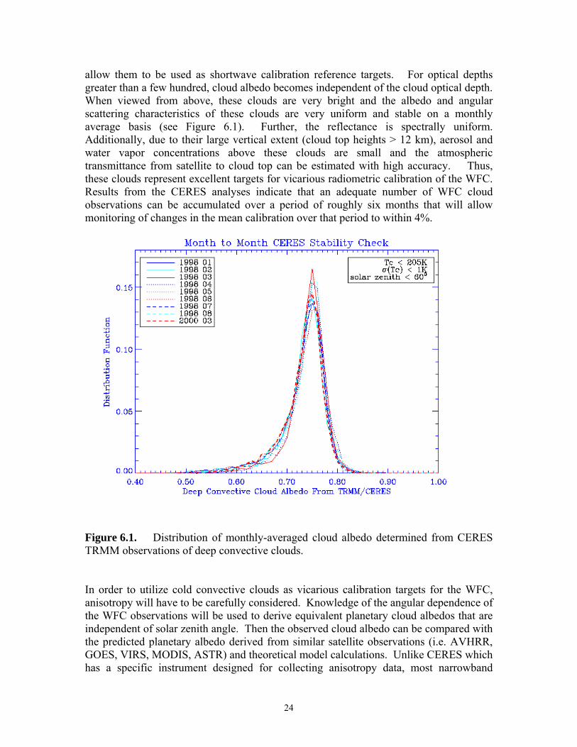
allow them to be used as shortwave calibration reference targets. For optical depths greater than a few hundred, cloud albedo becomes independent of the cloud optical depth. When viewed from above, these clouds are very bright and the albedo and angular scattering characteristics of these clouds are very uniform and stable on a monthly average basis (see Figure 6.1). Further, the reflectance is spectrally uniform. Additionally, due to their large vertical extent (cloud top heights > 12 km), aerosol and water vapor concentrations above these clouds are small and the atmospheric transmittance from satellite to cloud top can be estimated with high accuracy. Thus, these clouds represent excellent targets for vicarious radiometric calibration of the WFC. Results from the CERES analyses indicate that an adequate number of WFC cloud observations can be accumulated over a period of roughly six months that will allow monitoring of changes in the mean calibration over that period to within 4%.

Figure 6.1. Distribution of monthly-averaged cloud albedo determined from CERES TRMM observations of deep convective clouds. In order to utilize cold convective clouds as vicarious calibration targets for the WFC, anisotropy will have to be carefully considered. Knowledge of the angular dependence of the WFC observations will be used to derive equivalent planetary cloud albedos that are independent of solar zenith angle. Then the observed cloud albedo can be compared with the predicted planetary albedo derived from similar satellite observations (i.e. AVHRR, GOES, VIRS, MODIS, ASTR) and theoretical model calculations. Unlike CERES which has a specific instrument designed for collecting anisotropy data, most narrowband

25

instruments only perform cross-track scanning making it difficult to derive anisotropy models from these observations alone. As a result, a broadband-narrowband conversion scheme has been developed using CERES, VIRS, and MODIS observations on TRMM and Terra. Using this approach, it is possible to derive narrowband anisotropy models for the WFC from broadband models. 6.1.2 Radiometric Calibration Application Consider the solar radiance reflected by a deep convective cloud. As observed by any WFC pixel, p, this radiance is expressed as . Similarly, the bi-directional reflectance observed by any WFC pixel for this cloud is given by Rearranging terms and using the definition of the calibration constant, Cp, from Section 5.2.3, this expression can be written as . Therefore, if the cloud reflectance, ρcc,p, can be accurately characterized then cold tropical convective clouds could be used for determining the end-to-end radiometric calibration coefficient for the WFC. As shown by the CERES data, the cloud reflectance is very stable and we should be able to accurately characterize the angular variations using the well-calibrated shortwave MODIS channels. Although the extraterrestrial solar irradiance, So, is known to within 1 – 2 %, the absolute value is not required for determining the calibration constant. This also reduces the calibration errors due to uncertainty in knowledge of the WFC spectral band pass. Operationally, the time-dependent calibration coefficient, Cp, will be determined by combining and averaging tropical cloud measurements made over multiple orbits. To achieve the desired accuracy, averages of several months of measurements may be required. 6.1.3 Other Vicarious Approaches Vicarious calibration requires stable, homogeneous targets with relatively high reflectance. Additional potential calibration targets for the WFC include deserts, polar snow, and oceans.

]DNDN[GI~ opp,ccpp,cc −α=

oo

opp,ccp

p,ccS

]DNDN[Gµ

−πα=ρ

]DNDN[ρµC o

pp,cc

cc,pop

−π=

26

Deserts Well-characterized land surfaces may also be used as calibration targets under clear sky conditions. Deserts make good targets because they tend to be homogeneous over large regions and stable with time, but their angular scattering properties must be well characterized. Potential desert targets include portions of the Sahara desert in Algeria that have been characterized for use in calibrating the POLDER instrument and areas in the Australian desert which are uniform and have been, or could be, characterized. Desert targets also pose several potential problems for accurate calibration. For instance, it is not clear how accurately the scattering properties of the desert surfaces can be characterized, but probably nowhere close to the 2% level. Additionally, the presence of aerosol and water vapor can make accurate atmospheric transmissivity calculations problematic. POLDER claims a calibration to 4% accuracy using vicarious techniques, but in this case desert scenes are only used for calibrating the angular variation of the responsivity, not absolute radiometric calibration. Polar Snow Snow covered surfaces in the polar regions also could be used as vicarious calibration targets. Snow covered surfaces tend to be very homogeneous and offer the advantage that a large number of samples could be collected during most orbits. One difficulty in using snow surfaces as calibration targets is the solar zenith dependence varies with the age of the snow. In addition, the presence of Arctic haze and low level clouds can frequently contaminate the calibrations. A solar zenith dependence database for snow surfaces has been produced from MODIS Terra data. Oceans Ocean surfaces also might be useful calibration targets. In this case, the CALIPSO lidar can be used to identify clear ocean scenes with low aerosol loading. In contrast to cold convective clouds, deserts, and snow, these will be low-radiance scenes. At low wind speeds and outside of Sun glint regions, the oceans surface is extremely dark at 650 nm and the WFC signal will be dominated by Rayleigh scattering which is well-known. The small contribution from scattering off the ocean surface can be estimated with reasonable accuracy and the contributions from aerosols can be estimated from the lidar observations. 6.1.4 Cross-Calibration with MODIS and CERES Since MODIS has a well-calibrated shortwave channel centered very near 645 nm, it may be possible to use tropical convective clouds to transfer the MODIS calibration to the WFC. One potential difficulty is the differences in viewing geometry between CALIPSO and Aqua. As shown in Figure 6.2, the reflectance for viewing zenith angles between 0 – 5 degrees is very similar to those for viewing angles between 5 – 10 degrees. Therefore, if the CALIPSO and Aqua orbits are close, the reflectance should be almost identical. However, if the orbits differ significantly, then viewing zenith dependence needs to be considered. The narrowband angular reflectance characteristics of cold tropical clouds may be derived from MODIS measurements. Comparison of the WFC observations with the CERES broadband reflectance may also prove useful. For example, Figure 6.3 shows

27

Figure 6.2. Comparison of visible reflectance for viewing angles between 0–5o

and 5-10o. Figure 6.3. Comparison between CERES broadband and VIRS narrowband cloud reflectance (solid line represents model calculations with assumed particle shapes).

28

the relationship between CERES broadband and VIRS narrowband (650 nm) reflectance based on TRMM observations of ice clouds. The solar zenith angle in this case is between 42 – 48 degrees. The straight line in the figure is derived from model calculations with assumed particle shapes. Similar comparisons of the WFC data and the CERES Aqua broadband shortwave observations may provide useful calibration information. Again, however, viewing angle differences between the CALIPSO WFC and Aqua CERES may have to be considered. 6.2 Dark Current Offset The dark current offset, o

pDN , is essentially the thermally induced charge accumulated by each detector pixel when no light is present. Preflight values of these offsets were determined during ground testing of the WFC. However, radiation effects in space are expected to cause the dark current to increase over the lifetime of the mission. In addition, although the CCD focal plane temperature is controlled by a thermoelectric cooler (TEC), temperature fluctuations may occur due to strong thermal gradients across the spacecraft platform. Therefore, it is important that the dark current offset be monitored carefully on orbit. Nominally, dark frames are acquired during the nighttime portion of each orbit to calibrate the dark current offset in each pixel. Approximately 300 dark frames are acquired during each orbit. The Level 0 dark frame data has the same format as the daylight science data, but has a flag in the header record to distinguish it from daytime science data. Operationally, the dark frame data is processed as part of the Level 1 data processing and reported as the WFC Level 1 Calibration Data Product. The calibration data consists of the background count levels in each pixel for each frame. In addition, the mean count levels and standard deviations are calculated for each orbit. The calibration data is analyzed off-line to monitor changes in the dark current offset and identify defective pixels. Trends in the data are noted and the dark current file used in Level 1 processing is updated as necessary.

7. LEVEL 1 QUALITY CONTROL

7.1 Geolocation Verification Verification of the WFC pixel geolocation accuracy and an assessment of the spacecraft pointing will be performed using a coastline-crossing algorithm (Currey, 2002). This pointing assessment algorithm was first used on ERBE (Hoffman et al., 1987) and further refined in support of the CERES instrument Tropical Rainfall Measuring Mission (TRMM) (Currey et al., 1998). Validation of the geolocation process requires comparison of detected Earth features with a database containing the same features independently geolocated. For CALIPSO, clear coastline scenes will be analyzed to determine coastline-crossing locations. These are then compared with a coastline map to

29

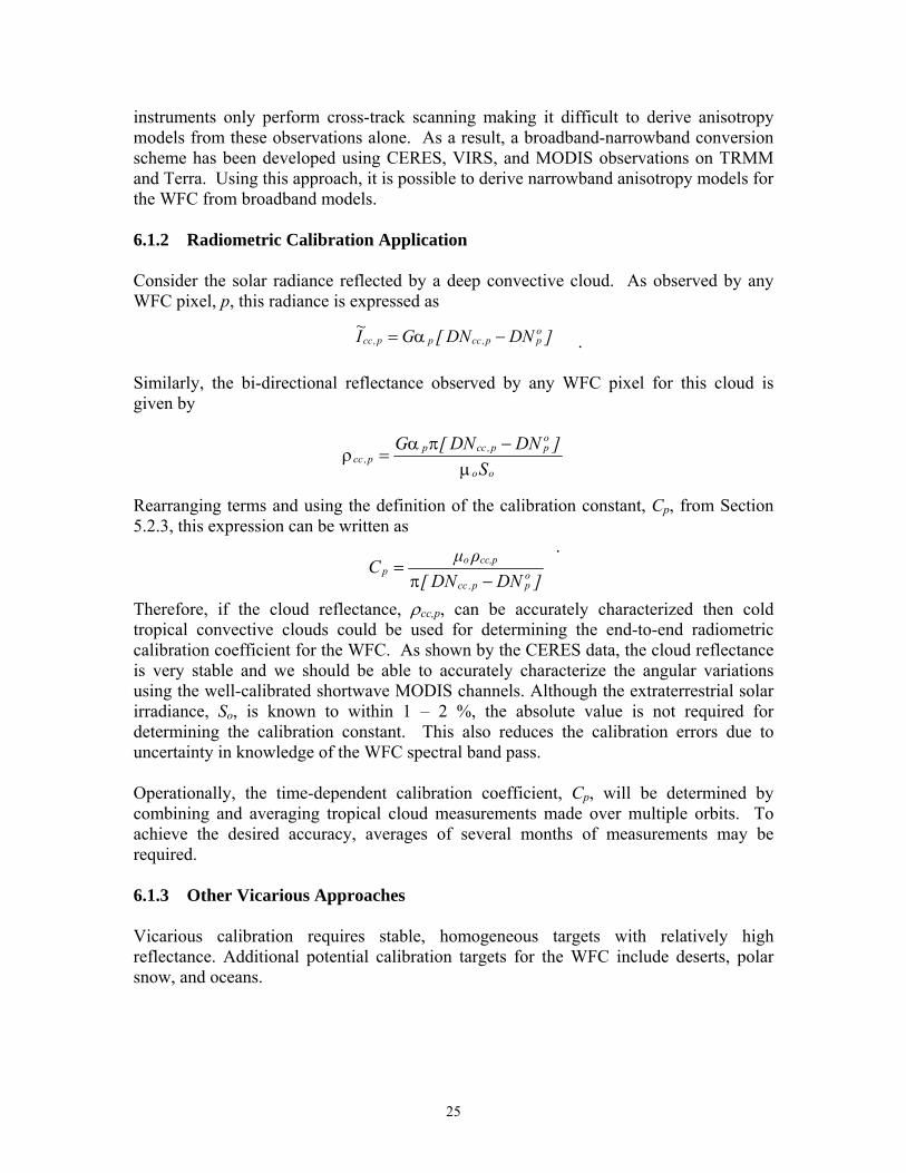
assess overall pointing accuracy. A large number of independently processed coastline scenes will be analyzed to detect systematic biases in the spacecraft along-track and cross-track coordinate system. 7.1.1 Coastline Crossing Algorithm As a detector scans across a high contrast scene, such as desert adjacent to ocean, a step response similar to Figure 7.1 is produced. The coastline signature is modeled using a cubic fit of four contiguous measurement samples

y i = ax i3 + bx i

2 + cx i + d where yi is the measured radiance and xi is pixel position (latitude or longitude). The equation coefficients are determined by solving the system of equations

⎥⎥⎥⎥

⎦

⎤

⎢⎢⎢⎢

⎣

⎡

dcba

=

1

42

43

4

32

33

3

22

23

2

12

13

1

1111

−

⎥⎥⎥⎥⎥

⎦

⎤

⎢⎢⎢⎢⎢

⎣

⎡

xxxxxxxxxxxx

⎥⎥⎥⎥

⎦

⎤

⎢⎢⎢⎢

⎣

⎡

4

3

2

1

yyyy

The inflection point, -b/3a, is considered to be the location of the coastline if it falls between x2 and x3 and the change in the observed radiance (or reflectance) exceeds a pre-defined threshold.

Figure 7.1. Determination of coastline crossing location.

30

The geolocation error for a scene is calculated by fitting an ensemble of detected crossings to a corresponding coastline map. The shift in geographical coordinates required to minimize the distance between the calculated coastline crossings and the coastline map is defined as the geolocation error for an individual scene. Figure 7.2 depicts an ensemble of crossings simulated from a digitized map of Baja, California with a bias of –1.2o longitude and 0.2o latitude. The downhill simplex minimization algorithm (Press et al., 1988) iteratively shifts the coastline in three separate directions until the differences between the calculated crossings and the map coastline are minimized. Geographic errors are transformed into spacecraft cross-track and along-track coordinates. Additional scenes are required to identify and track systematic biases in the instrument/satellite system.

Figure 7.2. Minimization technique to determine geolocation error. Figure 7.3 shows an example of this technique applied to a TRMM Visible and Infrared Scanner (VIRS) image of the western coast of Mexico taken January 3, 1998. Spacecraft heading is –31.6° relative to the equator. The minimum brightness temperature threshold in this case is 3 K. The coastline fitting technique minimizes 218 detected crossings to the World Data Bank II map database. The resulting longitude error of –0.0011° and latitude error of –0.0041o correspond to an along track error of 133 m and a cross track error of 455 m. VIRS pixel resolution is 2 km.

31

Figure 7.3. VIRS coastline detection example, Mexico, January 3, 1998

32

CALIPSO WFC geolocation verification will utilize two NOAA digital coastline reference maps: the Medium Resolution Digital Shoreline (MRDS) map and the World Vector Shoreline (WVS) map. The MRDS map is a digital compilation of 270 NOAA nautical charts covering the contiguous United States from the most up-to-date charts available from 1988-1992. The resultant average map scale is approximately 1:70,000 (~35-m resolution). The WVS map provides global coverage with a nominal scale of 1:250,000 (~125-m resolution). The National Imagery and Mapping Agency (NIMA) requires that 90% of all identifiable WVS shoreline features be located within 500 meters circular error of their true geographic positions referenced to the World Geodetic System (WGS) 84 Earth Model. The MRDS map will be used for analysis of WFC coastline scenes within the United States; otherwise the analyses will be based on WVS maps. Both map databases are available from an online site, the “Coastline Extractor,” hosted by the NOAA National Geophysical Data Center. 7.1.2 Algorithm Accuracy Considerations Two calculations contribute to the uncertainty of the coastline algorithm: 1) identification of coastline crossings in the WFC images, and 2) fitting the WFC coastline crossing ensembles to the reference coastline map. 7.1.2.1 Coastline Detection Errors The detector point spread function (PSF), coastline response model, and random sampling all affect the uncertainty of the calculated crossing location. Figure 7.4 depicts a number of theoretical one-dimensional PSFs with their corresponding step responses. Increments in the x-axis or along-scan direction are 0.01 pixels. The normalized PSFs vary from one to four pixels in width. The coastline truth is simulated with a step input at pixel index 100.

Figure 7.4. One dimensional PSFs and step response inflection point shifts.

0 100 200 3 0 0 0

0.1

0.2

0.3

0.4

0.5

0.6

0.7

0.8

0.9

1

0 100 200 3000

0.005

0.01

0.015

33

Inflection points are calculated from four equally spaced random samples. Calculated crossings are compared to the true simulated coastline at pixel index 100. Non-symmetric PSFs have shifts of 0.27 and 0.45 pixels with σ = 0.06 pixels. Table 7.1 summarizes the PSF coastline detection biases and uncertainties (N=100 random samples). The WFC PSF most closely resembles the first theoretical PSF in Table 7.1. For CALIPSO, each coastline crossing should be detected within 0.53 pixels (3σ) of the true coastline.

PSF Width (pixels)

Shift (pixels)

σ (pixels)

3σ (pixels)

1 0.000 0.176 0.528 2 0.000 0.098 0.294 3 0.266 0.055 0.165 4 0.446 0.064 0.192

Table 7.1. PSF step response coastline detection biases and uncertainties

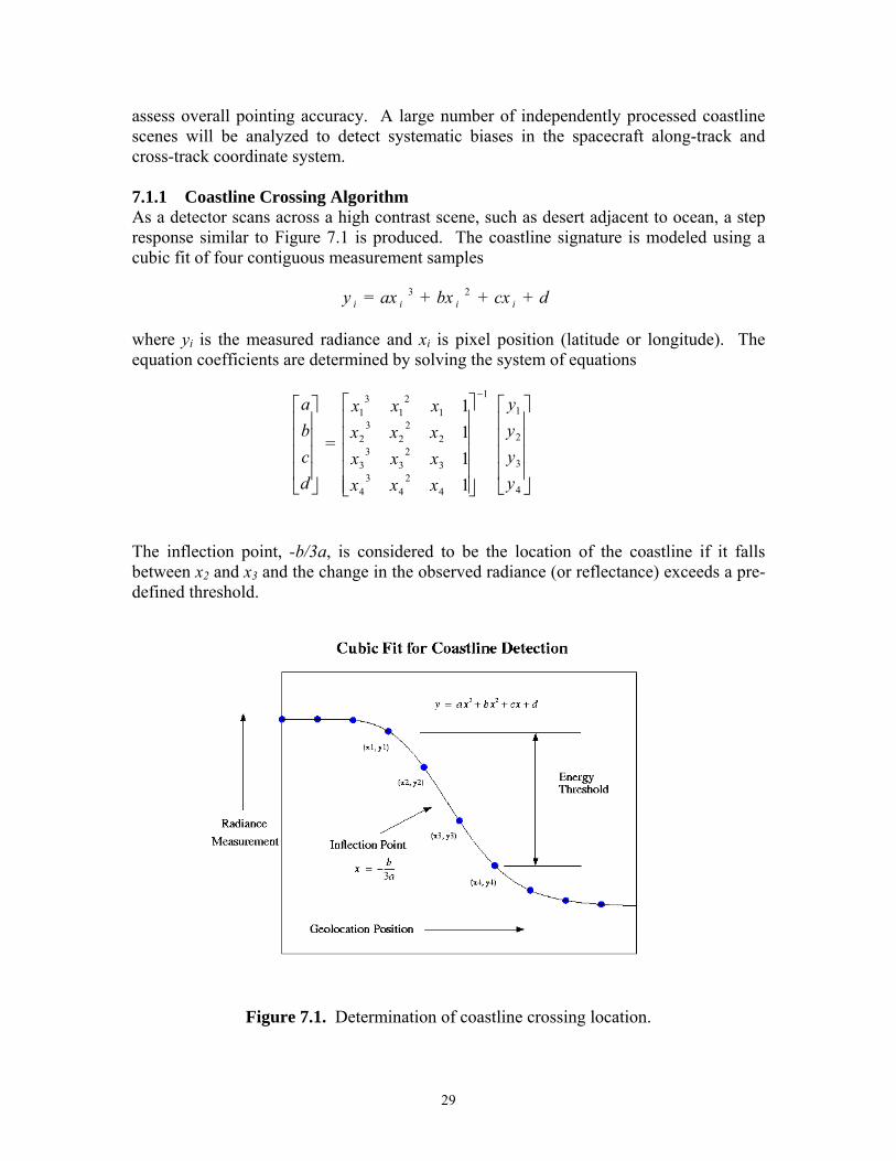
As a test case, a visible radiance land/water scene was generated using a radiative transfer model. This 1-m resolution dataset serves as the coastline truth. A convolution with the two-dimensional WFC PSF produces a simulated 125-m resolution, 5-km wide WFC scene. Figure 7.5 shows the 37 crossings detected from the 125-m data compared to the true coastline. Table 7.2 presents the along-track errors for the processed simulated WFC scene. The mean shift is 0.024 pixels (3 m) with 99.7% of the detected crossings within 0.28 pixels (35 m) of the true coastline. A mean negative shift indicates that the calculated crossings occur prior to the coastline map locations. To detect both along-track and cross-track errors, the minimization technique described in section 7.1.1 will be used. 7.1.2.2 Bias Determination Error The coastline detection algorithm essentially samples the shape of a coastline; the minimization process matches this shape to a reference map. The uncertainty in fitting the collection of WFC coastline crossings to the reference map is called the bias determination error. This section attempts to quantify the uncertainty of the bias determination algorithm and define map resolution and accuracy requirements. Table 7.3 depicts the bias determination accuracy when geographic biases are added to crossings simulated from a reference map, in this case a map of Baja, California containing 1158 values. Biases between the crossings and the map range from 1.2 degrees (~133 km) to .0001 degrees (~11 m). In all cases, except for the case of only 4 crossings, the correct bias is determined. The final average simplex shift indicates the magnitude and direction the crossings must be shifted in geographic coordinates to minimize the average crossing distance to the map. The simplex shift is the negative bias for a scene. The crossings are shifted back to their original map positions to within one meter (final difference). A fractional convergence tolerance, ftol, of .01 requires the three

34

simplex values to agree to within 1% of each other. Press et al. (1988) provides an excellent description of the downhill simplex method of minimization. The minimization process also works when the map resolution is less than the instrument pixel resolution. The ratio of map points per scene to crossings detected varies from 1 to 40 with accurate bias detection.

Figure 7.5. WFC scene simulated w/ 2D PSF convolution

Shift (pixels)

σ (pixels)

3σ (pixels)

-0.024

.084

.253

Table 7.2. Along-track errors for simulated WFC scene

X

Y

1000 2000 3000 4000 5000

500

1000

1500

2000

2500

3000

3500

4000

4500

Frame 001 26 Oct 2001 Pitts Simulation with & without PSFFrame 001 26 Oct 2001 Pitts Simulation with & without PSF

35

7.1.2.3 Geolocation Assessment Error The geolocation assessment accuracy is determined from the uncertainties of the coastline detection and bias determination algorithms. A theoretical estimate of the geolocation assessment accuracy can be calculated as follows: where σCD is the standard deviation of the coastline detection process (Table 7.1), σMAP is the uncertainty for an individual reference map point, NXINGS are the number of coastline crossings detected for a WFC scene, and NMAP are the number of reference coastline map points to which the ensemble distance is minimized. The WFC PSF most closely resembles the first theoretical PSF in Table 7.1, therefore the coastline detection uncertainty, σCD, is about 0.176 pixels or 21 m when using 125-m resolution WFC data. The bias determination uncertainty, σMAP, is determined from the reference coastline map accuracy. For the WVS coastline map, 90% of the map points are required to be within 500 m circular error of the true geographic position; therefore the WVS standard deviation, σMAP, equals 303 m. Using the WVS coastline map, WFC scenes with more than 70 coastline crossings should allow the geolocation error to be resolved to within about 100 m (3 σ). Although no accuracy numbers are provided with the MRDS map, the resolution is significantly better than the WVS map which should potentially allow geolocation errors to be resolved to less than 100 m when using coastline scenes from within the United States. 7.1.2.4 Post Launch Bias Monitoring During the first 90 days of the CALIPSO mission, an initial assessment of the geolocation accuracy will be performed using an interactive visualization tool, View_HDF (Lee, 2001), modified to support geolocation assessment. Partially clear coastal scenes will be analyzed by interactively shifting the reference coastline map overlay to match the WFC image data. Each month following, geolocation biases will be monitored and, if needed, be corrected in the production processing system. 7.2 Detection of Defective Pixels Pixels typically will fail in one of two ways: as a dead pixel that exhibits no charge or as a bright pixel that exhibits large charge independent of the incident illumination. Both of these pixel defects will be obvious in the image data. A dead pixel will appear as dark streak in the data while a bright pixel will appear as a bright stripe in the data. In addition, both types of pixel defects will be identified through statistical analysis of the dark frame data. Dead pixels will not affect adjacent pixels. Bright pixels will have essentially no effect on pixels in adjacent columns because the CCD has channel-stop regions to isolate columns from one another. However, charge from bright pixels may bleed into adjacent rows. If isolated pixels fail, they will be added to the bad pixel map and masked during

MAPMAP

XINGSCD

NN22

2 σσσ +=

36

Level 1 processing. If multiple pixel failures occur in the active row, then the target row will be moved. In the case of bright pixels, the target row will be shifted by at least 2 rows to reduce the bleeding effect. 7.3 Reflectance Statistics Statistics on the observed WFC reflectance will be generated for each orbit and reported as part of the Level 1 Data Product. The WFC data will be sorted into 5o solar zenith angle bins (0-5o, 5-10o, 10-15o, etc). For each solar zenith bin, the distribution of the observed WFC reflectance will be determined. These reflectance distributions will be compared with climatological statistics derived from MODIS data to provide an assessment of WFC data quality.

8. REFERENCES Release 5A SDP Toolkit Users Guide, ECS 333-CD-500-001, June 1999. Currey, C., Geolocation Assessment Algorithm for CALIPSO Using Coastline Detection,

NASA Technical Paper 2002-211956, 2002. Currey, C., L. Smith, and B. Neely, Evaluation of Clouds and the Earth’s Radiant Energy

System (CERES) scanner pointing accuracy using a coastline detection system, SPIE Conference on Earth Observing Systems III, San Diego, CA, July 1998.

Hoffman, L., W. Weaver, J. Kibler, Calculation and Accuracy of ERBE Scanner Measurement Locations, NASA Technical Paper 2670, 1987.

Lee, K., View_HDF User’s Guide, Version 3, 107 pp, 2001. http://eosweb.larc.nasa.gov/HPDOCS/view_hdf.html. Noerdlinger, P., Theoretical Basis for the SDP Toolkit Geolocation Package for the ECS

Project, ECS 445-TP-0002-002, May 1995. Press, W., B. Flannery, S. Teukolsky, and W. Vetterling, Numerical Recipes in C, Cambridge

University Press, Cambridge, 713 pp, 1998. Winker, D. M., M. P. McCormick, and R. Couch, An overview of LITE: NASA’s Lidar

In-space Technology Experiment, Proc. IEEE 84, 164-180, 1996.

37

Table 7.3. Scene Bias Determination Uncertainty

Number Xings

Lon, Lat Data Bias

(lon,lat)

Start Simplex (degrees)

Final Average Simplex Shift

(lon,lat)

Y[0] (m)

ftol Number Function

Calls

Number Simplex

Movements

Converge

1158 (÷1)

(0, 0) +/- 1.0 (-5.542168e-09, -6.309288e-08)

0.017 .001 217 97 yes

116 (÷10)

(0, 0) +/- 1.0 (-2.601026e-08, -5.096325e-08)

0.018 .01 1000 886 no

39 (÷30)

(0, 0) +/- 1.0 (-8.514351e-08, 1.417804e-07)

0.010 .01 128 64 yes

1158 (÷1)

(1.2, 0.2) +/- 2.0 (-1.199997e+00, -2.000005e-01)

0.364 .01 108 57 yes

116 (÷10)

(1.2, 0.2) +/- 2.0 (-1.199997e+00, -2.000002e-01)

0.405 .01 112 59 yes

29 (÷40)

(1.2, 0.2) +/- 2.0 (-1.199997e+00, -2.000004e-01)

0.268 .01 123 65 yes

1158 (÷1)

(-0.2, 1.2) +/- 2.0 (1.999972e-01, -1.200000e+00)

0.366 .01 113 59 yes

6 (÷200)

(-0.2, 1.2) +/- 2.0 (1.999969e-01, -1.200001e+00)

0.355 .01 134 67 yes

4 (÷300)

(-0.2, 1.2) +/- 2.0 (1.077308e+00, -2.743792e+00)

10710.0 .01 45 21 yes

58 (÷20)

(-0.5, -0.5) +/- 1.0 (5.000001e-01, 5.000002e-01)

0.016 .01 112 58 yes

58 (÷20)

(0.5, -0.5) +/- 1.0 (-4.999998e-01, 5.000002e-01)

0.018 .01 112 56 yes

58 (÷20)

(-0.01, -0.01) +/- 1.0 (9.994982e-03, 1.000023e-02)

0.433 .01 101 54 yes

58 (÷20)

(-0.01, -0.01) +/- 1.0 (-9.995032e-03, 9.999918e-03)

0.659 .01 108 57 yes

1158 (÷1)

(0.001, -0.001)

+/- 2.0 (-1.002690e-03, 1.000781e-03)

0.743 .01 93 50 yes

39 (÷30)

(0.001, -0.001)

+/- 2.0 (-1.005811e-03, 9.998169e-04)

0.657 .01 107 58 yes

1158 (÷1)

(0.0001, 0.0001)

+/- 0.5 (-1.049436e-04, -9.997992e-05)

0.717 .01 93 48 yes

58 (÷20)

(0.0001, 0.0001)

+/- 0.5 (-1.066786e-04, -9.977541e-05)

0.561 .01 99 51 yes

38