wide-field infrared survey explorer
TRANSCRIPT

Wide-field Infrared Survey Explorer
Subsystem Design Specification
Frame Co-addition
Version 8.385, 27-August-2010
Prepared by: Frank Masci
Infrared Processing and Analysis Center California Institute of Technology WSDC D-D019

2
Concurred By: Roc Cutri, WISE Science Data Center Manager Frank Masci, WISE Science Data Center Cognizant Engineer/Scientist

3
Revision History
Date Version Author Description
February 14, 2008 1.0 Frank Masci Initial Draft July 10, 2008 1.3 Frank Masci Implemented auto-tiling option
to support memory management for outlier detection
July 18, 2008 1.4 Frank Masci Implemented partitioning of frame lists to support memory management for outlier detection
August 19, 2008 1.5 Frank Masci Included ringing suppression algorithm to support HiRes
September 1, 2008 1.6 Frank Masci Implemented more robust frame background estimation when extended structure present. To support b’gnd matching and HiRes.
September 5, 2008 1.7 Frank Masci - Included -mcmprod switch to generate CFV and intensity cell images at each MCM iteration. - Also made box sizes for bmatch step more robust and avoid NaNs when computing extended source metrics
September 8, 2008 1.8 Frank Masci Added AWOD pad parameter: –pb_odet
October 25, 2008 1.9 Frank Masci Generated QA meta table and compute metrics
November 7, 2008 2.0 Frank Masci Implemented QA graphics files November 17, 2008 2.1 Frank Masci Included –wf option to control
inverse variance weighting. When on, leads to flux under-estimation for for bright srcs
January 28, 2009 2.2 Frank Masci Changed some for-loop notations in partitionme subroutine since syntax appears to conflict with PDL for some unknown reason
February 13, 2009 2.3 Frank Masci * Changed some for-loop notations in partitionme subroutine since syntax

4
appears to conflict with PDL. * Added subroutine to randomize input frame/mask lists prior to partitioning for outlier detection if “-partition” is set.
February 23, 2009 2.4 Frank Masci * Combined mask sub-mosaics into final mask if partitioning was triggered; update MAGZP and MAGZPUNC keys in input frame headers with global co-add values if tmatch performed. * Update MAGZP and MAGZPUNC keys in input frame headers with global co-add values if tmatch performed
May 20, 2009 2.6 Frank Masci Included new CL options -ip_odet and -is_odet as per AWOD vsn 1.6.
June 26, 2009 2.7 Frank Masci Compute median of input MAGZPUNCs instead of mean to protect against outliers; don't update MAGZPUNC in modified intensity frames since formally incorrect.
July 7, 2009 2.8 Frank Masci Included top-hat mosaic creation flag for use as MCM prior (-fp_coad); added -o9 output (cellcors from all iters) from first pass run of awaic, generated if -mcmprod option specified.
July 11, 2009 3.0 Frank Masci Include -ns_odet CL param. July 12, 2009 3.1 Frank Masci Included subroutine to expand
or blanket outlier regions. New CL params: -nei_odet, -nsz_odet, -exp_odet, -expodet
September 30, 2009 3.2 Frank Masci Added -ms_coad and -om_coad options to create mosaic mask and tag saturated and bad/unsaturated pixels.
October 1, 2009 3.3 Frank Masci Included NaN filtering in plane fitting for background matching.
October 20, 2009 3.4 Frank Masci Implemented drizzle option: -d_coad to match awaic vsn 4.5

5
November 2, 2009 3.5 Frank Masci Extensive HiRes functionality, new CL inputs: -h_coad; -oi_coad; -of_coad; -snu_coad; -snc_coad; -siggrid; also changed coadd exec to awaico in offline version.
November 2, 2009 3.6 Frank Masci Fix error-checking bug whereby creation of mask mosaic for n=1 is bypassed if any hires-related product or functionality is desired. Also added verbosity to SVB sub.
December 24, 2009 3.7 Frank Masci Fixed OutlierHist.svg QA plot when no outliers detected. Const. values caused crash.
January 18, 2010 3.8 Frank Masci Filter NaNs before computing block median for SVB.
February 13, 2010 4.0 Frank Masci Fixed cases when all int pixels of a QA partition are NaN'd and metrics croak.
March 6, 2010 4.1 Frank Masci Changed bmatch from switch to binary argument for easier calling in csh script.
March 11, 2010 4.2 Frank Masci * Added gausize, gausigm and flxbias as 1|0 binary CL options. * Added –bgrid param to compute robust frame background when extended structure detected in bmatch.
June 4, 2010 versioning now follows repository svn revision:
7.958
Frank Masci Implemented frame flagging due to excess outliers from e.g., moon-glow, SAA, saturation. Also make montage of jpegs of rejected frames
July 30, 2010 8.175 Frank Masci Implemented robust moon-masking algorithm using prior moon-masking
August 12, 2010 8.256 Frank Masci Added FITS metadata August 26, 2010 8.385 Frank Masci Current version – optimized
pixel-outlier and moon-rejection parameters in prep for prelim release.

6
Table of Contents
1. INTRODUCTION ......................................................................................................8
1.1 Purpose and Scope ...........................................................................................................8
1.2 Document Organization...................................................................................................8
1.3 Applicable Documents......................................................................................................9
1.4 Requirements..................................................................................................................10
1.5 Acronyms........................................................................................................................11
2 OVERVIEW .............................................................................................................13
3 INPUT/OUTPUT SUMMARY AND ASSUMPTIONS ...............................................15
3.1 I/O Specification.............................................................................................................15
3.2 Assumptions, Parameter Interplay, and Processing Details.........................................24
4 PREPARATORY STEPS ..........................................................................................28
4.1 Throughput (Gain) Matching ........................................................................................28
4.2 Frame Background/Level Matching..............................................................................29 4.2.1 Method 1: ‘robust’ tilted plane-fitting........................................................................30 4.2.2 Method 2: generic surface fitting with outlier rejection ..............................................31
5 FLAGGING OF MOON-GLOW FRAMES USING PRIOR MASK...........................32
6 OUTLIER DETECTION AND MASKING (AWOD).................................................35
6.1 Overview.........................................................................................................................35
6.2 Outlier Detection Implementation Details.....................................................................38 6.2.1 First Pass Computations.............................................................................................40 6.2.2 Second Pass Computations ........................................................................................43 6.2.3 Optimization Options ................................................................................................45 6.2.4 Frame-based outlier rejection.....................................................................................48
7 CO-ADDITION USING PRF INTERPOLATION .....................................................49
7.1 Advantages and Pitfalls of PRF-Interpolation ..............................................................52

7
8 CO-ADDITION USING OVERLAP-AREA WEIGHTING AND DRIZZLE ..............53
9 EXTENSION TO RESOLUTION ENHANCEMENT ................................................55
9.1 The Maximum Correlation Method ..............................................................................56
9.2 The CFV Diagnostic .......................................................................................................60
9.3 HiRes Uncertainties........................................................................................................62 9.3.1 a posteriori (data-derived) estimates..........................................................................62 9.3.2 Uncertainties from propagating priors........................................................................65 9.3.3 Signal-to-Noise Ratio Images ....................................................................................65
9.4 Ringing Suppression.......................................................................................................66
9.5 Noise Suppression Algorithm.........................................................................................68
9.6 HiRes in Practice............................................................................................................69
10 NAN’ING LOW DEPTH-OF-COVERAGE REGIONS............................................70
11 QUALITY ASSURANCE ........................................................................................70
11.1 Graphics........................................................................................................................74
12 USAGE EXAMPLES ..............................................................................................75
13 TESTING................................................................................................................75
14 LIENS .....................................................................................................................76

8
1. INTRODUCTION
1.1 Purpose and Scope This Subsystem Design Specification (SDS) document describes the basic requirements, assumptions, definitions, software-design details, algorithms, QA, and necessary interfaces for the COADD subsystem of the WISE Science Data System (WSDS). It is used to trace the incremental development of this subsystem, and contains sufficient detail to allow future modification or maintenance of the software by developers other than the original developer. framecoadder is a script that drives the COADD subsystem of the WISE Science Data System (WSDS). It is principally used to generate WISE Atlas Image products, but is generic enough for use on any astronomical image data that supports the FITS and WCS standards. It is a Perl script that threads together the various co-addition modules: AWAIC and AWOD (written in ANSI-compliant C), and contains functionality for background and throughput matching, moon-contamination flagging, resolution enhancement (HiRes), and Quality Assurance (QA). Throughout this document, the names “AWAIC”, framecoadder, or wframecoadder are used interchangeably. The HiRes functionality is not used in the generation of WISE Atlas Image products. It can be executed offline using the equivalent, publicly available AWAIC tool (for details, see http://wise2.ipac.caltech.edu/staff/fmasci/awaicpub.html). Overall, framecoadder performs the following steps, each of which can be turned on/off using command-line switches.
1. Throughput (gain) matching to equalize input photometric calibration zero-points and derive a single zero-point for the output co-add;
2. Background (offset) matching between frames to equalize levels;
3. Dynamic flagging of frames due to moon contamination;
4. Outlier pixel-detection and rejection (AWOD module), with subsequent frame-flagging
based on number of pixel-outliers per frame;
5. Frame co-addition (AWAIC module). HiRes’ing is optional;
6. QA metrics, plots and co-add uncertainty consistency checks. 1.2 Document Organization This document is organized along the major themes of Requirements; Other Software Interfaces; Assumptions; Functional Descriptions and Dependencies; Input/Output; Algorithm Descriptions; Testing; and Liens. The material contained in this document represents the current understanding
9
of the capabilities of the major WISE systems and sub-systems. Areas that require further analysis are noted by TBD (To Be Determined). 1.3 Applicable Documents
• WSDC Functional Requirements Document WSDC D-R001 (FRD – Level 4 Requirements): http://web.ipac.caltech.edu/staff/roc/wise/docs/WSDC_Functional_Requirements_all.pdf
• WSDS Functional Design Document WSDC D-D001 (FDD):
http://web.ipac.caltech.edu/staff/roc/wise/docs/WSDS_FDD_v1.pdf
• WSDC Science Data Quality Assurance Plan WSDC D-M004 (QAP): http://web.ipac.caltech.edu/staff/roc/wise/docs/QA_Plan_WSDC_2007-03-01.pdf
• Software Interface Specification (SIS) WSDC D-I101 – Frame Processing Mask:
http://web.ipac.caltech.edu/staff/fmasci/home/wise/InstruCal01.txt
• Software Interface Specification (SIS) WSDC D-I102 – Input Frame WCS FITS Header Keywords: http://web.ipac.caltech.edu/staff/fmasci/home/wise/SFPWrap01.txt
• Software Interface Specification (SIS) WSDC D-I121 – Level-3 (Atlas Image) QA
metadata: http://web.ipac.caltech.edu/staff/fmasci/home/wise/QAoutput_fco07.txt
• Proposed WISE Image Atlas Specifications (reviewed at Oct ’07 Science Team meeting): http://web.ipac.caltech.edu/staff/fmasci/home/wise/Atlas_image_spec_v1.2.pdf
• Atlas Image sky-tiling geometry:
http://web.ipac.caltech.edu/staff/fmasci/home/wise/tiling.html • Frame Co-addition Peer Review presentation (11/15/2007):
http://web.ipac.caltech.edu/staff/fmasci/home/wise/Co-addition_PeerReview.pdf
• Frame Co-addition Peer Review Report WSDC D-A001 (summary of 11/15/2007 Peer Review): http://spider.ipac.caltech.edu/staff/fmasci/home/wise/awaic_peerreview_report.pdf
• Frame Co-addition Critical Design Review (01/30/2008):
http://web.ipac.caltech.edu/staff/fmasci/home/wise/Co-addition_CDRJan08.pdf • Invited Talk on AWAIC: ADASS XVIII (11/04/2008, Quebec City):
http://web.ipac.caltech.edu/staff/fmasci/home/wise/adass08_talk.pdf

10
• Paper on AWAIC (for ADASS XVIII conference): http://web.ipac.caltech.edu/staff/fmasci/home/wise/awaic_adass08.pdf
• Overview on AWAIC with examples:
http://web.ipac.caltech.edu/staff/fmasci/home/wise/awaic.html • Example co-adds from a WSDS Processed simulation (v1.0 system release):
http://web.ipac.caltech.edu/staff/fmasci/home/wise/MidLatSimMosaics2.html • Example co-adds from 2MASS and Spitzer observations of the South Ecliptic Pole
(SEP): http://web.ipac.caltech.edu/staff/fmasci/home/wise/sep_mosaics.html • Examples/analysis from AWOD: A WISE Outlier Detector:
http://web.ipac.caltech.edu/staff/fmasci/home/wise/awod.html • A Simple Background Matcher (Bmatch):
http://web.ipac.caltech.edu/staff/fmasci/home/wise/bmatch.html
• WISE Science Team Meeting Presentation (04/19/2010): http://wise2.ipac.caltech.edu/proj/fmasci/AWAIC_STmtgApr10.pdf
• Moon-frame flagging proposal for multi-frame processing: http://wise2.ipac.caltech.edu/proj/fmasci/mooning.html
1.4 Requirements Below we summarize the requirements pertaining to the format, properties and quality of the final release WISE Atlas Image products. These are from the WSDC Functional Requirements Document (§1.3).
- L4WSDC-001: The WSDC shall produce a digital Image Atlas that combines multiple survey exposures at each position on the sky.
- L4WSDC-021: The images in the final WISE Image Atlas shall be re-sampled to a common pixel grid at all wavelengths.
- L4WSDC-022: The photometric calibration of the final WISE Image Atlas shall be tied to the photometric calibration of the final WISE Source Catalog.
- L4WSDC-023: The WSDC shall make all WISE image data available in accordance to the Flexible Image Transport (FITS) astronomical data standard.
- L4WSDC-026: The WSDC shall generate and archive coverage maps that show the number of independent observations that go into each pixel of the Image Atlas images in each band. The coverage numbers shall take into account focal plan coverage and losses due to poor data quality, low responsivity and/or high noise masked pixels, and pixels lost because of cosmic rays and other transient events.

11
- L4WSDC-051: The WSDC shall make the WISE catalog and image products available to the community via the internet through appropriate web-based tools.
- L4WSDC-053: The WSDC shall make the Image Atlas and Catalog products accessible to the astronomical community in collaboration with the NASA/IPAC Infrared Science Archive (IRSA) to ensure long-term availability beyond the end WISE missions operations and data processing phase, and to insure interoperability with other NASA mission archives.
- L4WSDC-060: The WSDC archive shall provide a web-based interface to enable selection, display and retrieval of any or all single-epoch images and combined Atlas Images based on position or time of observation for the purpose of quality assurance, validation and analysis. The goal shall be to select on any image metadata parameter.
- L4WSDC-078: The WISE science data products shall use the International Celestial Reference System (ICRS) to describe the positions and motions of celestial bodies. WISE astrometry shall be mapped into the ICRS using the 2MASS All-Sky Point Source Catalog as the primary astrometric reference.
- L4WSDC-084: The WISE Image Atlas shall be constructed by combining all available science images covering the sky. This does not include image pixels rejected because of low responsivity, high dark current or read noise, transient behavior such as charged particle impacts, or scattered light due to moon proximity.
- L4WSDC-086: The web-based interface to the WISE Image Atlas shall allow the user to view and retrieve an image in any of the four WISE bands with any specified center (tangent point) and any size up to at least 1° × 1°.
1.5 Acronyms 2-D Two-Dimensional 3-D Three-Dimensional ADASS Astronomical Data Analysis Software and Systems ANSI American National Standards Institute AWAIC A WISE Astronomical Image Co-adder AWOD A WISE Outlier Detector Bmatch Background matching CDR Critical Design Review CFV Correction Factor Variance COADD Co-Adder subsystem COBE COsmic Background Explorer COV depth-of-COVerage CPU Central Processing Unit CROTA2 Coordinate ROTAtion about axis 2 (W.of.N convention) DN Data Number DRAM Dynamic Random Access Memory E-W East-West FDD Functional Design Document FRD Functional Requirements Document

12
FITS Flexible Image Transport System FOV Field-Of-View GB Giga-Byte HIRES HIgh RESolution (sometimes written as HiRes) HST Hubble Space Telescope I/O Input / Output ICal Instrumental Calibration ICRS International Celestial Reference System INT INTensity IPAC Infrared Processing and Analysis Center IR Infra-Red IRAC Infra-Red Array Camera IRAS Infra-Red Astronomical Satellite IRSA NASA/IPAC Infra-Red Science Archive ISO International Organization for Standardization JPL Jet Propulsion Laboratory JPEG Joint Photographic Experts Group format Jy Jansky MAD Median Absolute Deviation MAGZP MAGnitude Zero Point MAGZPUNC MAGnitude Zero Point UNCertainty MB Mega-Byte MCM Maximum Correlation Method MED MEDian MOPEX Mosaicking and Point source EXtraction N-S North-South NaN Not-a-Number NEP North Ecliptic Pole ODET Outlier Detection PA Position Angle (E.of.N convention) PC Personal Computer PDL Perl Data Language PRF Point Response Function PSF Point Spread Function PTILE PercentTILE QA Quality Assurance QAP Quality Assurance Plan RAM Random Access Memory RL Richardson-Lucy algorithm RMS Root-Mean-Square fluctuation RSS Root-Sum-Squared SAA South Atlantic Anomaly SDS Subsystem Design Specification SEP South Ecliptic Pole

13
SIP Simple Imaging Polynomial SIS Subsystem Interface Specification S/N Signal-to-Noise SNR Signal-to-Noise Ratio (same as S/N) SUTR Sample-Up-The-Ramp SVB Slowly Varying Background SVG Scalable Vector Graphics format TBD To Be Determined TBR To Be Resolved Tmatch Throughput matching 2MASS Two Micron All Sky Survey UNC UNCertainty WCS World Coordinate System W? WISE band number: ? = 1, 2, 3, or 4 (~3.4, 4.6, 12.1, 22.2 µm) WISE Wide-field Infrared Survey Explorer WSDC WISE Science Data Center WSDS WISE Science Data System
2 OVERVIEW
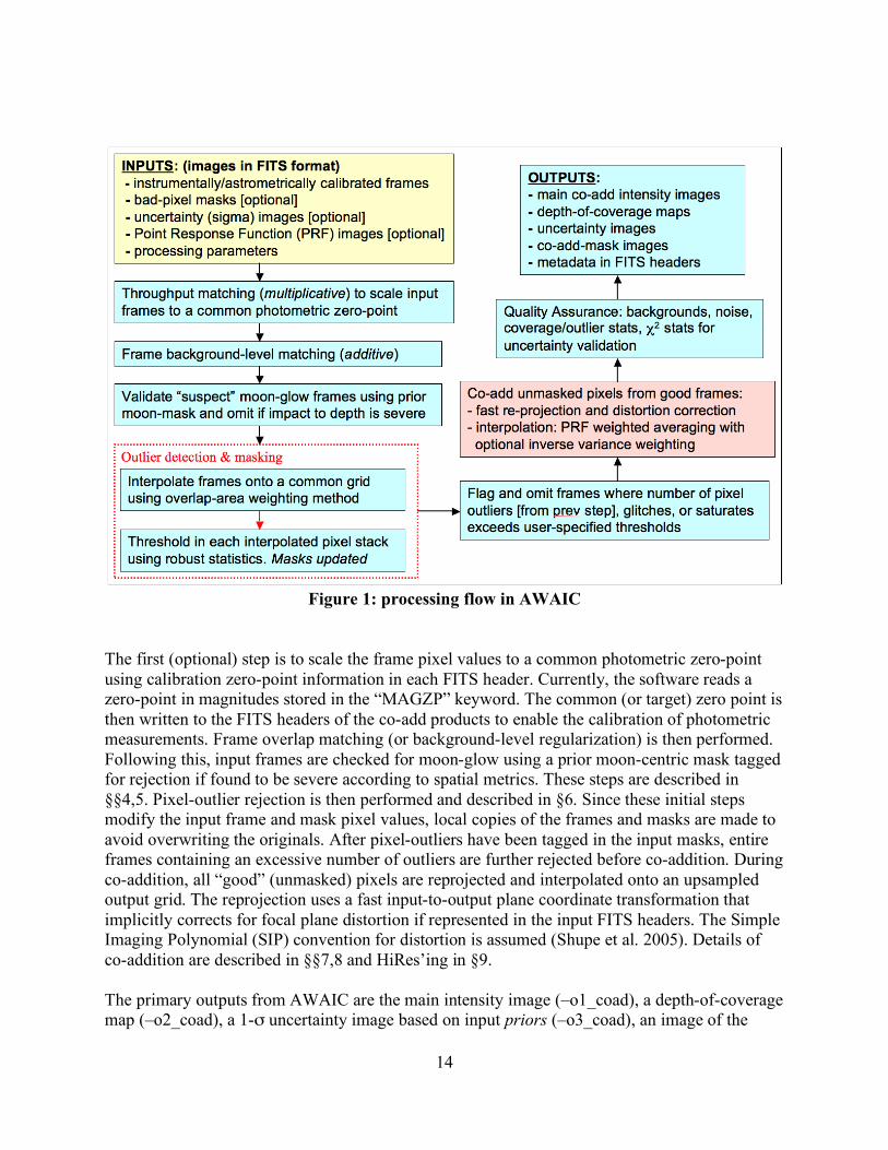
WISE shall downlink image data frames consisting of 1024 × 1024 pixels for bands 1, 2 and 3 with a projected size of 2.75 arcsec/pixel, and 512 × 512 pixels for band 4 with a size of 5.5 arcsec/pixel. This corresponds to image dimensions of ≈ 47 × 47 arcmin on the sky for all bands. The goal of image co-addition is to optimally combine a set of (usually dithered) exposures to create an accurate representation of the sky, given that all instrumental signatures, glitches, and cosmic-rays have been properly removed. By “optimally”, we mean a method which maximizes the signal-to-noise ratio (SNR) given prior knowledge of the statistical distribution of the input measurements. Figure 1 gives an overview of the main steps in AWAIC. The co-addition (and optional HiRes’ing) step is shown in the red box. All steps are expanded below. It is assumed that the input science frames (specified by –imglist) have been preprocessed to remove instrumental signatures and their pointing refined in some WCS using an astrometric catalog. Accompanying bad-pixel masks (–msklist) and prior-uncertainty frames (–unclist) are optional. The frames are assumed to overlap with some predefined footprint (or tile) on the sky. This also defines the dimensions of the co-add products. The uncertainty frames store 1-σ values for each pixel. These are expected to be initiated upstream, e.g., from a noise model specific to the detector and then propagated and updated as the instrumental calibrations are applied. The uncertainties are used for optional inverse-variance weighting of the input measurements and for computing co-add flux uncertainties. If bad-pixel masks are specified, a bit-string template (–m_coad) is used to select which conditions to flag against. The corresponding pixels in the science frames are then omitted from co-addition.
14
Figure 1: processing flow in AWAIC
The first (optional) step is to scale the frame pixel values to a common photometric zero-point using calibration zero-point information in each FITS header. Currently, the software reads a zero-point in magnitudes stored in the “MAGZP” keyword. The common (or target) zero point is then written to the FITS headers of the co-add products to enable the calibration of photometric measurements. Frame overlap matching (or background-level regularization) is then performed. Following this, input frames are checked for moon-glow using a prior moon-centric mask tagged for rejection if found to be severe according to spatial metrics. These steps are described in §§4,5. Pixel-outlier rejection is then performed and described in §6. Since these initial steps modify the input frame and mask pixel values, local copies of the frames and masks are made to avoid overwriting the originals. After pixel-outliers have been tagged in the input masks, entire frames containing an excessive number of outliers are further rejected before co-addition. During co-addition, all “good” (unmasked) pixels are reprojected and interpolated onto an upsampled output grid. The reprojection uses a fast input-to-output plane coordinate transformation that implicitly corrects for focal plane distortion if represented in the input FITS headers. The Simple Imaging Polynomial (SIP) convention for distortion is assumed (Shupe et al. 2005). Details of co-addition are described in §§7,8 and HiRes’ing in §9. The primary outputs from AWAIC are the main intensity image (–o1_coad), a depth-of-coverage map (–o2_coad), a 1-σ uncertainty image based on input priors (–o3_coad), an image of the

15
outlier locations (–om_odet), and optionally if the overlap-area interpolation method was used, an image of the data-derived uncertainty computed from the standard deviation in each interpolated pixel stack and appropriately scaled by the depth-of-coverage (–o4_coad). Additional ancillary products are generated under HiRes’ing. AWAIC also produces a wealth of Quality Assurance (QA) metrics over pre-specified regions of the co-add footprint (the latter is only possible in the WISE automated pipeline). These include background noise estimates, coverage and outlier statistics, and metrics to validate co-add flux uncertainties using χ2 tests. A summary of QA outputs is given in §11. Liens are summarized in §14.
3 INPUT/OUTPUT SUMMARY AND ASSUMPTIONS
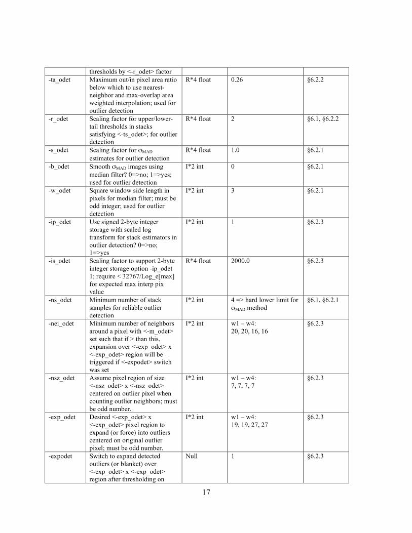
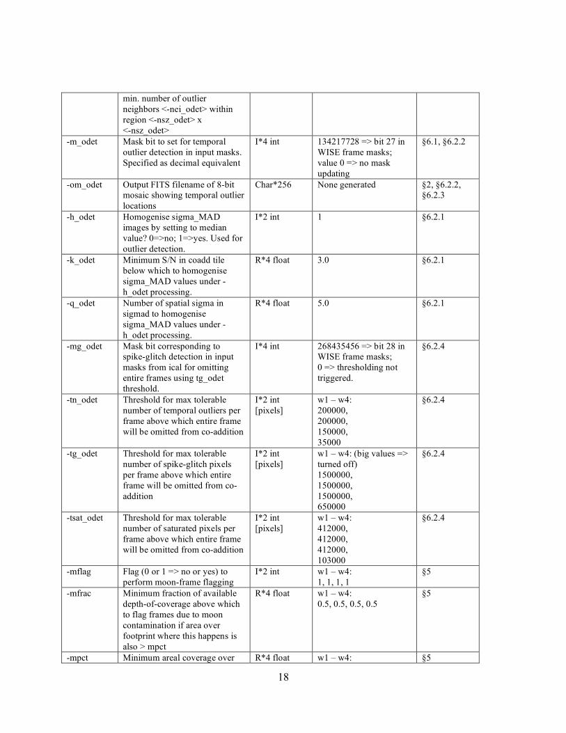
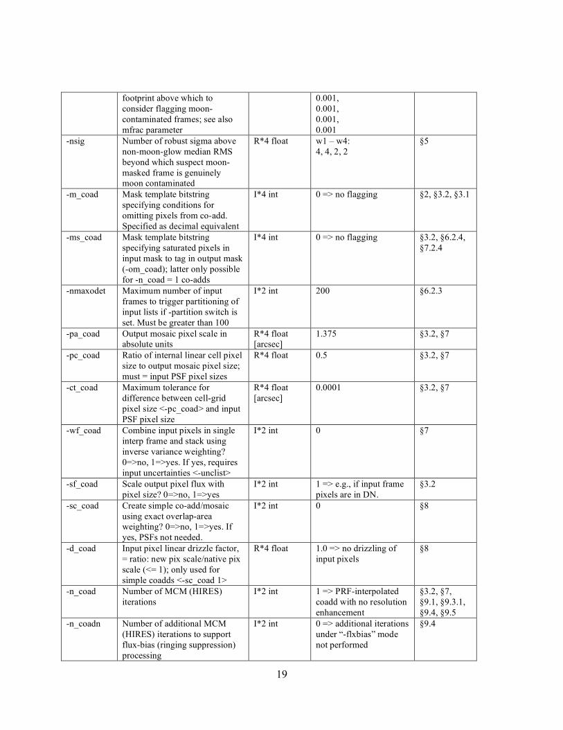
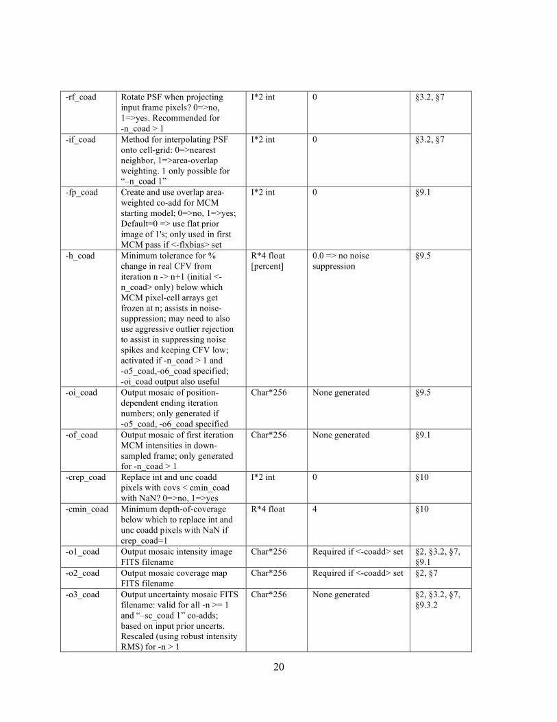
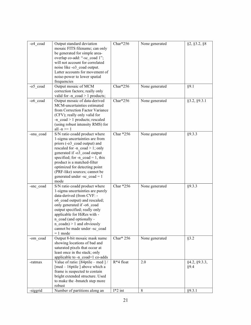
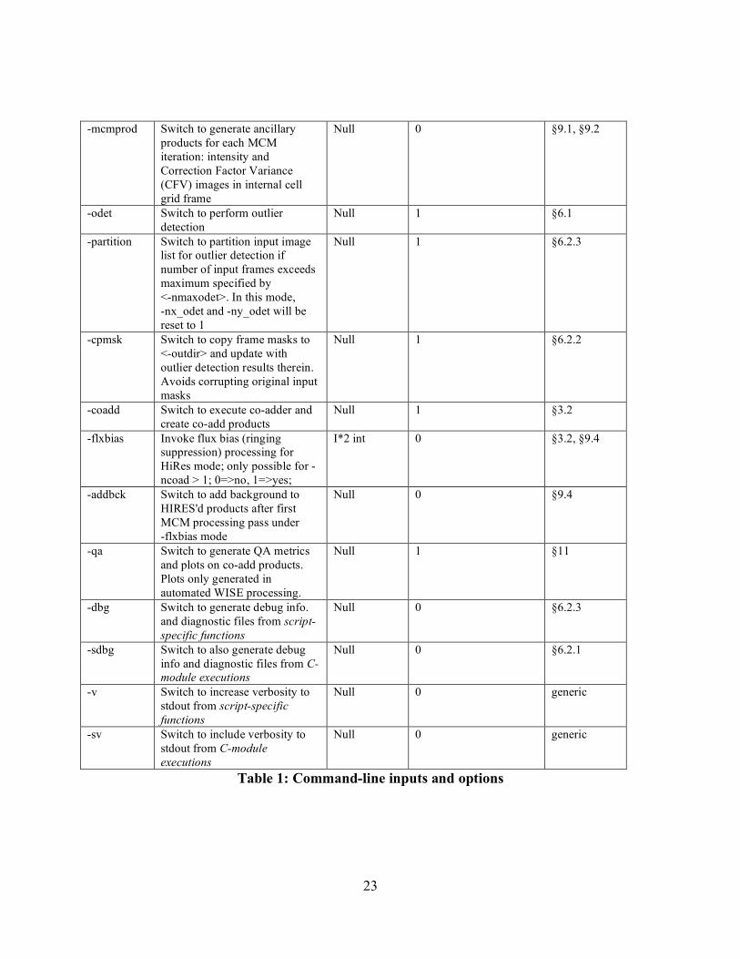
3.1 I/O Specification framecoadder is a Perl script that takes all of its input from the command-line. This command-line can be set-up and executed via a shell script. Prior to parsing the command-line, default values for the optional input parameters are assigned. All parameters are checked for validity and that they’re specified in the correct combination. Assumptions on input data formats are summarized in §3.2. Table 1 summarizes all command-line inputs, their purpose, data-type and units where applicable, default assignments, and section(s) in this document where you can find more information. Command-line inputs suffixed by “_odet” in Table 1 are specific to outlier detection. Inputs suffixed by “_coad” are specific to co-addition and/or HiRes’ing. All other inputs are generic to overall processing. Option Description Data-type,
[units] Default More info.
-imglist Input text file name containing list of pre-calibrated 32-bit / pixel FITS intensity images
Char*256 Required input §2, §3.2
-unclist Input text file name containing list of 32-bit / pixel FITS (1-sigma) uncertainty images
Char*256
None used §2, §3.2
-msklist Input text file name containing list of 32-bit / pixel (long int) FITS mask images
Char*256
None used §2, §3.2
-moonmeta Input frame metadata table containing prior moon-flag information for each band
Char*256 No moon-contamination flagging performed
§5
-psflist Input text file name containing list of focal-plane dependent PSF images. Only searched for if <-psfdir> below not specified.
Char*256
<psfdir> and <-basepsf> first used if specified. If <-psflist> also absent, area-overlap method <-sc_coad> is used
§3.2, §7
-psfdir Input pathname containing PSF Char*256 <-psflist> used §3.2

16
files -basepsf Input generic base filename of
PSF for N x N frame grid, for constructing focal-plane dependent PSFs
Char*256
<-psflist> used §3.2
-outdir Pathname for intermediate files and working directory
Char*256 Required input §4.1, §6.2.2, §6.2.3, §9.1, §9.2
-qadir Pathname for output QA diagnostic files and plots. Only used in automated WISE processing
Char*256 –outdir <path> §11
-archdir Pathname for archivable products and metadata
Char*256
–outdir <path> §11
-qameta Output filename for QA meta-data. Will be written under path specified by <-archdir>
Char*256 meta-coadd.tbl §11
-qagrid Number of partitions N along an axis of co-add footprint for computing QA metrics within N x N square regions
I*2 int 3 §11
-sizeX E-W mosaic dimension for crota2 = 0
R*4 float [degrees]
Required input §3.2, §6.2
-sizeY N-S mosaic dimension for crota2 = 0
R*4 float [degrees]
Required input §3.2, §6.2
-ra Right Ascension of mosaic center
R*4 float [degrees]
Required input §3.2, §6.2
-dec Declination of mosaic center R*4 float [degrees]
Required input §3.2, §6.2
-rot Mosaic position angle in terms of CROTA2: +Y axis W of N: 0 ≤ rot < 360
R*4 float [degrees]
0.0 §3.2, §6.2
-pa_odet Output interpolation grid pixel scale for outlier detection; recommend: ≥ 0.5 * input native pixel scale
R*4 float [arcsec]
Required if <-odet> set §6.2
-pb_odet Additional padding to add around mosaic grid for outlier detection; recommend: of order PRF size for co-addition
R*4 float [arcsec]
0 => possible outliers outside nominal mosaic boundary may contribute to co-add
§6.2
-nx_odet Number of tiles along X dimension of mosaic for outlier detection
I*2 int 1 => whole mosaic §6.2, §6.2.2, §6.2.3
-ny_odet Number of tiles along Y dimension of mosaic for outlier detection
I*2 int 1 => whole mosaic §6.2, §6.2.2, §6.2.3
-tl_odet Lower-tail threshold in number of sigma for outlier detection
R*4 float w1 – w4: 8, 8, 7, 7
§6.1, §6.2.2, §6.2.3, §9.5
-tu_odet Upper-tail threshold in number of sigma for outlier detection
R*4 float w1 – w4: 8, 8, 7, 7
§6.1, §6.2.2, §6.2.3, §9.5
-ts_odet Minimum "(median bckgnd) / sigma" value for stack above which to rescale <-tl> and <-tu>
R*4 float w1 – w4: 8, 8, 8, 8
§6.1, §6.2.2
17
thresholds by <-r_odet> factor -ta_odet Maximum out/in pixel area ratio
below which to use nearest-neighbor and max-overlap area weighted interpolation; used for outlier detection
R*4 float 0.26 §6.2.2
-r_odet Scaling factor for upper/lower-tail thresholds in stacks satisfying <-ts_odet>; for outlier detection
R*4 float 2 §6.1, §6.2.2
-s_odet Scaling factor for σMAD estimates for outlier detection
R*4 float 1.0 §6.2.1
-b_odet Smooth σMAD images using median filter? 0=>no; 1=>yes; used for outlier detection
I*2 int 0 §6.2.1
-w_odet Square window side length in pixels for median filter; must be odd integer; used for outlier detection
I*2 int 3 §6.2.1
-ip_odet Use signed 2-byte integer storage with scaled log transform for stack estimators in outlier detection? 0=>no; 1=>yes
I*2 int 1 §6.2.3
-is_odet Scaling factor to support 2-byte integer storage option -ip_odet 1; require < 32767/Log_e[max] for expected max interp pix value
R*4 float 2000.0 §6.2.3
-ns_odet Minimum number of stack samples for reliable outlier detection
I*2 int 4 => hard lower limit for σMAD method
§6.1, §6.2.1
-nei_odet Minimum number of neighbors around a pixel with <-m_odet> set such that if > than this, expansion over <-exp_odet> x <-exp_odet> region will be triggered if <-expodet> switch was set
I*2 int w1 – w4: 20, 20, 16, 16
§6.2.3
-nsz_odet Assume pixel region of size <-nsz_odet> x <-nsz_odet> centered on outlier pixel when counting outlier neighbors; must be odd number.
I*2 int w1 – w4: 7, 7, 7, 7
§6.2.3
-exp_odet Desired <-exp_odet> x <-exp_odet> pixel region to expand (or force) into outliers centered on original outlier pixel; must be odd number.
I*2 int w1 – w4: 19, 19, 27, 27
§6.2.3
-expodet Switch to expand detected outliers (or blanket) over <-exp_odet> x <-exp_odet> region after thresholding on
Null 1 §6.2.3
18
min. number of outlier neighbors <-nei_odet> within region <-nsz_odet> x <-nsz_odet>
-m_odet Mask bit to set for temporal outlier detection in input masks. Specified as decimal equivalent
I*4 int
134217728 => bit 27 in WISE frame masks; value 0 => no mask updating
§6.1, §6.2.2
-om_odet Output FITS filename of 8-bit mosaic showing temporal outlier locations
Char*256 None generated §2, §6.2.2, §6.2.3
-h_odet Homogenise sigma_MAD images by setting to median value? 0=>no; 1=>yes. Used for outlier detection.
I*2 int 1 §6.2.1
-k_odet Minimum S/N in coadd tile below which to homogenise sigma_MAD values under -h_odet processing.
R*4 float 3.0 §6.2.1
-q_odet Number of spatial sigma in sigmad to homogenise sigma_MAD values under -h_odet processing.
R*4 float 5.0 §6.2.1
-mg_odet Mask bit corresponding to spike-glitch detection in input masks from ical for omitting entire frames using tg_odet threshold.
I*4 int 268435456 => bit 28 in WISE frame masks; 0 => thresholding not triggered.
§6.2.4
-tn_odet Threshold for max tolerable number of temporal outliers per frame above which entire frame will be omitted from co-addition
I*2 int [pixels]
w1 – w4: 200000, 200000, 150000, 35000
§6.2.4
-tg_odet Threshold for max tolerable number of spike-glitch pixels per frame above which entire frame will be omitted from co-addition
I*2 int [pixels]
w1 – w4: (big values => turned off) 1500000, 1500000, 1500000, 650000
§6.2.4
-tsat_odet Threshold for max tolerable number of saturated pixels per frame above which entire frame will be omitted from co-addition
I*2 int [pixels]
w1 – w4: 412000, 412000, 412000, 103000
§6.2.4
-mflag Flag (0 or 1 => no or yes) to perform moon-frame flagging
I*2 int
w1 – w4: 1, 1, 1, 1
§5
-mfrac Minimum fraction of available depth-of-coverage above which to flag frames due to moon contamination if area over footprint where this happens is also > mpct
R*4 float w1 – w4: 0.5, 0.5, 0.5, 0.5
§5
-mpct Minimum areal coverage over R*4 float w1 – w4: §5
19
footprint above which to consider flagging moon-contaminated frames; see also mfrac parameter
0.001, 0.001, 0.001, 0.001
-nsig Number of robust sigma above non-moon-glow median RMS beyond which suspect moon-masked frame is genuinely moon contaminated
R*4 float w1 – w4: 4, 4, 2, 2
§5
-m_coad Mask template bitstring specifying conditions for omitting pixels from co-add. Specified as decimal equivalent
I*4 int 0 => no flagging §2, §3.2, §3.1
-ms_coad Mask template bitstring specifying saturated pixels in input mask to tag in output mask (-om_coad); latter only possible for -n_coad = 1 co-adds
I*4 int 0 => no flagging §3.2, §6.2.4, §7.2.4
-nmaxodet Maximum number of input frames to trigger partitioning of input lists if -partition switch is set. Must be greater than 100
I*2 int 200 §6.2.3
-pa_coad Output mosaic pixel scale in absolute units
R*4 float [arcsec]
1.375 §3.2, §7
-pc_coad Ratio of internal linear cell pixel size to output mosaic pixel size; must = input PSF pixel sizes
R*4 float 0.5 §3.2, §7
-ct_coad Maximum tolerance for difference between cell-grid pixel size <-pc_coad> and input PSF pixel size
R*4 float [arcsec]
0.0001 §3.2, §7
-wf_coad Combine input pixels in single interp frame and stack using inverse variance weighting? 0=>no, 1=>yes. If yes, requires input uncertainties <-unclist>
I*2 int 0 §7
-sf_coad Scale output pixel flux with pixel size? 0=>no, 1=>yes
I*2 int 1 => e.g., if input frame pixels are in DN.
§3.2
-sc_coad Create simple co-add/mosaic using exact overlap-area weighting? 0=>no, 1=>yes. If yes, PSFs not needed.
I*2 int 0 §8
-d_coad Input pixel linear drizzle factor, = ratio: new pix scale/native pix scale (<= 1); only used for simple coadds <-sc_coad 1>
R*4 float 1.0 => no drizzling of input pixels
§8
-n_coad Number of MCM (HIRES) iterations
I*2 int 1 => PRF-interpolated coadd with no resolution enhancement
§3.2, §7, §9.1, §9.3.1, §9.4, §9.5
-n_coadn Number of additional MCM (HIRES) iterations to support flux-bias (ringing suppression) processing
I*2 int 0 => additional iterations under “-flxbias” mode not performed
§9.4
20
-rf_coad Rotate PSF when projecting input frame pixels? 0=>no, 1=>yes. Recommended for -n_coad > 1
I*2 int 0 §3.2, §7
-if_coad Method for interpolating PSF onto cell-grid: 0=>nearest neighbor, 1=>area-overlap weighting. 1 only possible for “–n_coad 1”
I*2 int 0 §3.2, §7
-fp_coad Create and use overlap area-weighted co-add for MCM starting model; 0=>no, 1=>yes; Default=0 => use flat prior image of 1's; only used in first MCM pass if <-flxbias> set
I*2 int 0 §9.1
-h_coad Minimum tolerance for % change in real CFV from iteration n -> n+1 (initial <-n_coad> only) below which MCM pixel-cell arrays get frozen at n; assists in noise-suppression; may need to also use aggressive outlier rejection to assist in suppressing noise spikes and keeping CFV low; activated if -n_coad > 1 and -o5_coad,-o6_coad specified; -oi_coad output also useful
R*4 float [percent]
0.0 => no noise suppression
§9.5
-oi_coad Output mosaic of position-dependent ending iteration numbers; only generated if -o5_coad, -o6_coad specified
Char*256 None generated §9.5
-of_coad Output mosaic of first iteration MCM intensities in down-sampled frame; only generated for -n_coad > 1
Char*256 None generated §9.1
-crep_coad Replace int and unc coadd pixels with covs < cmin_coad with NaN? 0=>no, 1=>yes
I*2 int 0 §10
-cmin_coad Minimum depth-of-coverage below which to replace int and unc coadd pixels with NaN if crep_coad=1
R*4 float
4 §10
-o1_coad Output mosaic intensity image FITS filename
Char*256 Required if <-coadd> set §2, §3.2, §7, §9.1
-o2_coad Output mosaic coverage map FITS filename
Char*256 Required if <-coadd> set §2, §7
-o3_coad Output uncertainty mosaic FITS filename: valid for all -n >= 1 and “–sc_coad 1” co-adds; based on input prior uncerts. Rescaled (using robust intensity RMS) for -n > 1
Char*256 None generated §2, §3.2, §7, §9.3.2
21
-o4_coad Output standard deviation mosaic FITS filename; can only be generated for simple area-overlap co-add: “-sc_coad 1”; will not account for correlated noise like -o3_coad output. Latter accounts for movement of noise-power to lower spatial frequencies
Char*256 None generated §2, §3.2, §8
-o5_coad Output mosaic of MCM correction factors; really only valid for -n_coad > 1 products;
Char*256 None generated §9.1
-o6_coad Output mosaic of data-derived MCM-uncertainties estimated from Correction Factor Variance (CFV); really only valid for -n_coad > 1 products; rescaled (using robust intensity RMS) for all -n >= 1
Char*256 None generated §3.2, §9.3.1
-snu_coad S/N ratio coadd product where 1-sigma uncertainties are from priors (-o3_coad output) and rescaled for -n_coad > 1; only generated if -o3_coad output specified; for -n_coad = 1, this product is a matched-filter optimized for detecting point (PRF-like) sources; cannot be generated under -sc_coad = 1 mode
Char *256 None generated §9.3.3
-snc_coad S/N ratio coadd product where 1-sigma uncertainties are purely data-derived (from CVF: -o6_coad output) and rescaled; only generated if -o6_coad output specified; really only applicable for HiRes with -n_coad (and optionally -n_coadn) > 1 and obviously cannot be made under -sc_coad = 1 mode
Char *256 None generated §9.3.3
-om_coad Output 8-bit mosaic mask name showing locations of bad and saturated pixels that occur at least once in the stack; only applicable to -n_coad=1 co-adds
Char* 256 None generated §3.2
-ratmax Value of ratio: [84ptile – med ] / [med – 16ptile ] above which a frame is suspected to contain bright extended structure. Used to make the -bmatch step more robust
R*4 float 2.0 §4.2, §9.3.3, §9.4
-siggrid Number of partitions along an I*2 int 8 §9.3.1

22
axis of final coadd product for finding smallest robust RMS to support uncertainty coadd rescaling both from priors (-o3_coad) and/or CFV (-o6_coad)
-svbgrid Number of partitions along an axis of native input frame for median SVB computation to support HiRes with -flxbias processing and generation of S/N coadds: -snu_coad and/or -snc_coad for -n_coad >= 1
I*2 int 5 §9.3.3, §9.4
-gausize Linear size of Gaussian smoothing kernel as a multiple (factor) of median-filter window length defined by NAXIS/svbgrid
R*4 float 3.0 §9.3.3
-gausigm sigma_x, sigma_y of Gaussian smoothing kernel as a multiple (factor) of -gausize
R*4 float 0.3 §9.3.3
-magzp Global photometric zero-point value to scale to
R*4 float [mag]
Required if <-tmatch> set. Current defaults: 20.5, 19.5, 17.5, 13.0
§4.1
-magzpun 1-sigma uncertainties in magzp, for writing to coadd FITS headers
R*4 float [mag]
Uses median of input frame magzpuncs if these are not null. Otherwise, current defaults are: 0.0002, 0.0002, 0.0005, 0.0013.
§4.1
-tmatch Switch to perform throughput (gain) matching of input frames
Null 0 §4.1
-bmatch Optional background (offset) matching of input frames; 0=>no, 1=>yes;
I*2 int 0 §4.2, §9.3.3, §9.4
-bmeth Background-matching / regularization method: 0 => robust planar fit; 1 => higher order surface fit to clipped data; only applicable if -bmatch switch was set
I*2 int 1 §4.2.2
-order Order of polynomial to fit for -bmeth=1
I*2 int 2 §4.2.2
-bgrid Size of bgrid x bgrid for partitioning frame and computing median pixel values for input into surface fitting routine for bmeth=1
I*2 int 9 §4.2.2
-clsig Number (N) of robust sigma to clip high tail from mode and replace with mode+N*sigma before partitioning and fitting surface under bmeth=1
R*4 float
0.5 §4.2.2
23
-mcmprod Switch to generate ancillary products for each MCM iteration: intensity and Correction Factor Variance (CFV) images in internal cell grid frame
Null 0 §9.1, §9.2
-odet Switch to perform outlier detection
Null 1 §6.1
-partition Switch to partition input image list for outlier detection if number of input frames exceeds maximum specified by <-nmaxodet>. In this mode, -nx_odet and -ny_odet will be reset to 1
Null 1 §6.2.3
-cpmsk Switch to copy frame masks to <-outdir> and update with outlier detection results therein. Avoids corrupting original input masks
Null 1 §6.2.2
-coadd Switch to execute co-adder and create co-add products
Null 1 §3.2
-flxbias Invoke flux bias (ringing suppression) processing for HiRes mode; only possible for -ncoad > 1; 0=>no, 1=>yes;
I*2 int 0 §3.2, §9.4
-addbck Switch to add background to HIRES'd products after first MCM processing pass under -flxbias mode
Null 0 §9.4
-qa Switch to generate QA metrics and plots on co-add products. Plots only generated in automated WISE processing.
Null 1 §11
-dbg Switch to generate debug info. and diagnostic files from script-specific functions
Null 0 §6.2.3
-sdbg Switch to also generate debug info and diagnostic files from C-module executions
Null 0 §6.2.1
-v Switch to increase verbosity to stdout from script-specific functions
Null 0 generic
-sv Switch to include verbosity to stdout from C-module executions
Null 0 generic
Table 1: Command-line inputs and options

24
3.2 Assumptions, Parameter Interplay, and Processing Details Below we list the assumptions pertaining to the format, size, and content of the image inputs. Some recommendations on parameter usage are also given. Many of these are sanity checked during early execution of framecoadder. If not satisfied, the program aborts with a message and a non-zero exit status written to standard error.
• The input lists of intensity images (–imglist), masks (–msklist), and uncertainty images (–unclist) must all have the same number of filenames listed in one-to-one correspondence.
• All input frames are expected to overlap with some predefined footprint on the sky with WCS/dimensions/pixel scale defined by –ra, –dec, –rot, –sizeX, –sizeY, and –pa_coad. This footprint also defines the dimensions of the output co-add products. Note the output interpolation grid for outlier detection uses the same WCS/dimensions but uses a pixel scale specified by –pa_odet. If the bulk of your input frames do not overlap with this footprint, you'll be wasting precious memory [primarily during the outlier detection step].
• All image inputs are in FITS format. • All input intensity, mask and uncertainty images are expected to have the same native
pixel scale (but ΔX ≠ ΔY is allowed); the same projection type (CTYPE header keywords); the same NAXIS1, NAXIS2 values (with NAXIS1 ≠ NAXIS2 allowed); and the same EQUINOX.
• If FOV-distortion information is available, this must be represented in the FITS headers of the intensity images using the Simple Imaging Polynomial (SIP) convention with the WCS keywords CDELT1, CDELT2, CROTA2 encoded in CD matrix format.
• It is recommended that all image pixel scales (either from CDELT or CD keywords) be represented in the FITS headers to at least 8 significant figures.
• The only projection types recognized by the software are: TAN, SIN, ZEA, STG and ARC. These are specific to the fast plane-to-plane reprojection algorithm.
• To exercise the PRF-weighted averaging option, i.e., for either co-addition (–n_coad = 1) or HiRes’ing (–n_coad > 1), a list of PRFs must be specified. This can be either one PRF applicable to the entire focal plane of the detector frames, or, multiple PRFs if the PRF is non-isoplanatic. The PRFs can be specified explicitly using an input list (–psflist), or by providing the path to their location and a PRF base-filename: –psfdir and –basepsf respectively. The script first checks if –psfdir and –basepsf were specified. If not, it checks for –psflist. If –psflist is not specified, the processing diverts to making a simple co-add using overlap-area weighting (i.e., –sc_coad is forced “on”).
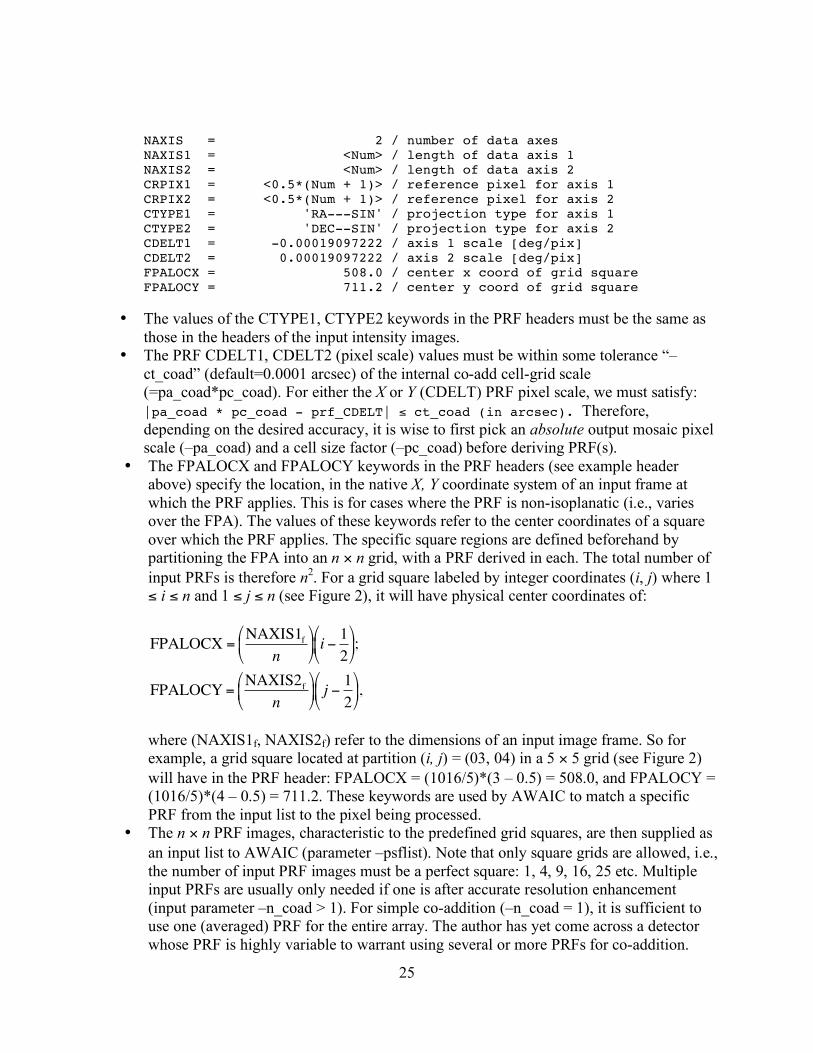
• The input PRF images (e.g., from –psflist) must all be of the same size (i.e., their NAXIS1, NAXIS2 values the same) and have the same pixel scale (CDELT1, CDELT2 keywords). An example of a minimal FITS header for an input PRF is as follows (where the CDELT* and FPALOC* values are not realistic). See below on how to derive the FPALOC* keywords.
SIMPLE = T / file does conform to FITS standard BITPIX = -32 / number of bits per data pixel
25
NAXIS = 2 / number of data axes NAXIS1 = <Num> / length of data axis 1 NAXIS2 = <Num> / length of data axis 2 CRPIX1 = <0.5*(Num + 1)> / reference pixel for axis 1 CRPIX2 = <0.5*(Num + 1)> / reference pixel for axis 2 CTYPE1 = 'RA---SIN' / projection type for axis 1 CTYPE2 = 'DEC--SIN' / projection type for axis 2 CDELT1 = -0.00019097222 / axis 1 scale [deg/pix] CDELT2 = 0.00019097222 / axis 2 scale [deg/pix] FPALOCX = 508.0 / center x coord of grid square FPALOCY = 711.2 / center y coord of grid square
• The values of the CTYPE1, CTYPE2 keywords in the PRF headers must be the same as
those in the headers of the input intensity images. • The PRF CDELT1, CDELT2 (pixel scale) values must be within some tolerance “–
ct_coad” (default=0.0001 arcsec) of the internal co-add cell-grid scale (=pa_coad*pc_coad). For either the X or Y (CDELT) PRF pixel scale, we must satisfy: |pa_coad * pc_coad - prf_CDELT| ≤ ct_coad (in arcsec). Therefore, depending on the desired accuracy, it is wise to first pick an absolute output mosaic pixel scale (–pa_coad) and a cell size factor (–pc_coad) before deriving PRF(s).
• The FPALOCX and FPALOCY keywords in the PRF headers (see example header above) specify the location, in the native X, Y coordinate system of an input frame at which the PRF applies. This is for cases where the PRF is non-isoplanatic (i.e., varies over the FPA). The values of these keywords refer to the center coordinates of a square over which the PRF applies. The specific square regions are defined beforehand by partitioning the FPA into an n × n grid, with a PRF derived in each. The total number of input PRFs is therefore n2. For a grid square labeled by integer coordinates (i, j) where 1 ≤ i ≤ n and 1 ≤ j ≤ n (see Figure 2), it will have physical center coordinates of:
!
FPALOCX =NAXIS1
f
n
"
# $
%
& ' i (
1
2
"
# $
%
& ' ;
FPALOCY =NAXIS2
f
n
"
# $
%
& ' j (
1
2
"
# $
%
& ' ,
where (NAXIS1f, NAXIS2f) refer to the dimensions of an input image frame. So for example, a grid square located at partition (i, j) = (03, 04) in a 5 × 5 grid (see Figure 2) will have in the PRF header: FPALOCX = (1016/5)*(3 – 0.5) = 508.0, and FPALOCY = (1016/5)*(4 – 0.5) = 711.2. These keywords are used by AWAIC to match a specific PRF from the input list to the pixel being processed.
• The n × n PRF images, characteristic to the predefined grid squares, are then supplied as an input list to AWAIC (parameter –psflist). Note that only square grids are allowed, i.e., the number of input PRF images must be a perfect square: 1, 4, 9, 16, 25 etc. Multiple input PRFs are usually only needed if one is after accurate resolution enhancement (input parameter –n_coad > 1). For simple co-addition (–n_coad = 1), it is sufficient to use one (averaged) PRF for the entire array. The author has yet come across a detector whose PRF is highly variable to warrant using several or more PRFs for co-addition.
26
• The PRFs must be volume-normalized to unity. This is internally checked. The sum of all PRF values in an input PRF image must not differ from unity by more than 1.0E-06. This tolerance is hard-coded.
• The maximum linear footprint dimension supported by the image projection libraries in AWAIC is 16°. However, one is likely to run out of memory first (depending on the output pixel scales chosen) before the necessary arrays are allocated. The reason for this maximum is that for dimensions exceeding this, the SIN and TAN projections (the most common types) will give pixel scale distortions of >1% and >2% respectively at the extremities relative to the footprint center.
• The internal cell to output mosaic pixel size ratio (command-line parameter –pc_coad) must be expressible in the form 1/integer, where integer = 1, 2, 3…, and lie within the range: 0.2 ≤ pc_coad ≤ 1.0. The lower limit is hard-coded.
• The input value for –pa_coad must satisfy: 0.1*minrawscale ≤ pa_coad ≤ minrawscale, where minrawscale = min[input_image_CDELT1, input_image_CDELT2] and the input_image_CDELTs are pixel scales in the input raw images.
• The output grid pixel scale for outlier detection, –pa_odet <in arcsec> must satisfy: minscale ≤ pa_odet ≤ maxscale, where minscale = sqrt[MINAREAR*inp_image_CDELT1*inp_image_CDELT2]; maxscale = sqrt[inp_image_CDELT1*inp_image_CDELT2], and MINAREAR = 0.1. The inp_image_CDELTs are pixel scales in the input intensity images. Therefore, the grid pixel scale is constrained by the ratio of output/input pixel area.
• The input pixel mask FITS images if specified, are expected to have a BITPIX=32 (i.e., 32-bit signed integer format). However, only the first 31 bits (excluding the sign bit) are used in processing. Masks with BITPIX=16 or 8 or even -32 (floating point) can still be stored. Only the integer part of the float will be stored for input masks with BITPIX=-32.
• The input fatal bit-string template specification for co-addition or HiRes’ing: –m_coad allows one to flag pixels according to certain conditions/criteria. The maximum value allowed is 231 = 2147483647. If this value is specified, then all pixels with values ≥20 in the input masks will be omitted from co-addition or subsequent HiRes’ing.
• There is another input bit-string for tracking saturated pixels in input frames: –ms_coad [0 ≤ value ≤ 231]. This requires knowledge of which bits define saturation in the input masks. This information is used to tag saturated locations with value “100” in an output 8-bit mask with filename specified by –om_coad. Bad pixels specified by the –m_coad bit-string (see above) are also tagged in this mask and assigned value “1”. For a stack of frames, non-zero values in the –om_coad mask imply that a saturated or bad pixel occurred at least once at that sky location in the stack. This mask is only generated for PRF-interpolated co-adds (–n_coad 1). Furthermore, if the –ms_coad saturation bit-string is specified, this must be included in the overall bad-pixel bit-string specified by: –m_coad.
• The area-overlap weighting interpolation method (command-line option –if_coad = 1) can only be invoked when (i) generating a PRF-weighted (–n_coad = 1) co-add, and (ii) when no rotation of the input PRF during re-projection is desired (command line option –rf_coad = 0). The interpolation method will default to the “nearest neighbor” method (–

27
if_coad = 0) if either rotation of the PRF is specified (–rf_coad = 1), or, resolution enhancement is desired (–n_coad > 1).
• It is recommended that the “nearest neighbor” method with rotation included (–if_coad = 0 and –rf_coad = 1) be used when performing resolution enhancement.
• If “nearest neighbor” interpolation is used and the output mosaic pixel scale (from –pa_coad) is not a fraction expressible as (1/integer)*input image pixel scale where integer = 1, 2, 3…, then systematic patterns in the output depth-of-coverage map may result. These are normalized out of the intensity images since there is an implicit division by the coverage at every location (see formalism in §7). However, to minimize systematic variations in the coverage map when nearest neighbor interpolation is used, it is advised that: (i) a new output mosaic pixel scale be chosen that satisfies the (1/integer)*input image pixel scale criterion, and (ii) that the input PRFs are sampled to a pixel scale ≤ 0.25 × input image pixel scale. If you are adamant on using a specific output mosaic pixel scale, then the more robust (but slower) area-overlap weighting PRF-interpolation method (–if_coad 1) can be used.
• The pixel units in the output intensity co-add (–o1_coad) and corresponding uncertainty images (–o3_coad or –o4_coad or –o6_coad) reflect the input image units and can be scaled using the –sf_coad <scale> parameter. For example, if the input image units are in Data Number (DN or counts), one may want to re-scale these according to pixel area so that the total counts in a photometric aperture are conserved.
• Any of the four major processing steps can be turned off/on using command line switches: background (offset) matching: –bmatch; throughput (gain) matching: –tmatch; co-addition or HiRes’ing: –coad; quality assurance: –qa. This functionality is useful for testing purposes.
• The –flxbias switch to support ringing suppression in HiRes (§9.4) will also need the –bmatch (background matching) switch specified in order to trigger the extended structure detection algorithm (see §4.2). This special processing allows the frame SVB to be replaced by a constant equal to the minimum median background over all –svbgrid × –svbgrid partitions of a frame if extended structure is detected through the –ratmax parameter.
• If the –mcmprod switch (for generating HiRes ancillary products) is specified (§9.1-9.2), you will also need to specify the –o5_coad and –o6_coad output product filenames.

28
Figure 2: Example of a 5 × 5 partition of an input frame for defining FPA position-dependent PRFs with an indexing scheme for computing the FPALOCX and FPALOCY keywords (see §3.2).
4 PREPARATORY STEPS
4.1 Throughput (Gain) Matching The first (optional) step is to scale the frame pixel values to a common photometric zero-point using calibration zero-point information in each input frame FITS header. This step is only necessary if the calibration zero-point (i.e., the raw data units [e.g., DN] to absolute units [e.g., Jy] conversion factor) varies amongst your input frames. This step can be controlled via the –tmatch switch in framecoadder. If the –tmatch switch is set, the software reads a zero-point in magnitudes stored as the “MAGZP” keyword in each science frame FITS header (e.g., as used in 2MASS and WISE image products). If throughput matching is desired and this keyword is not present in the header, it can be derived using:

29
!
MAGZP = Mtrue "Minst
= "2.5log10
ftrue
f0
#
$ %
&
' ( + 2.5log10 DN[ ]
= 2.5log10
f0
c
#
$ % &
' ( ,
where Mtrue and Minst are the true and instrumental magnitudes of a calibrator source, DN (Data Number) are the raw image pixel counts of the calibrator source from photometry (with background subtraction), ftrue is its “true” flux density (e.g., Jy), f0 is the flux corresponding to magnitude zero, and c = ftrue/DN = the “DN-to-[Jy]” conversion factor (or whatever absolute units are involved). Some instruments (e.g., on Spitzer) only report values for c, in which case it would need to be converted to some corresponding relative MAGZP as above. Let’s label the MAGZP in an input frame FITS header as magzpi. Given a common (or target) zero-point magzpc specified via –magzp <input>, the pixels (pold) in frame i are rescaled according to:
!
pnew = pold100.4 magzpc "magzpi( ) .
The same operation is performed on the input uncertainty frames if specified. The target zero point (magzpc) is then written to the FITS headers of co-add image products as “MAGZP”. This enables the calibration of photometric measurements off a co-add. Also, since this step modifies the input frame pixel values (likewise for the background level-matching step described below), local copies of the frames (intensities and uncertainties) and are made to avoid overwriting the originals. The modified frames are created under the directory specified by –outdir. If uncertainties in the zero-points “MAGZPUNC” are also provided in the input frame headers, they are median-combined to derive an effective MAGZPUNC to accompany the co-add MAGZP. If these are null (“-999” or absent), the value specified by input parameter –magzpun is used as the output coadd MAGZPUNC. 4.2 Frame Background/Level Matching Frame exposures taken at different times usually show variations in background levels due to, for example, instrumental transients, changing environments, scattered and stray light. The goal is to obtain seamless (and/or smooth) transitions between frames near their overlap regions prior to co-addition. We will want to equalize background levels from frame to frame, but at the same time preserve natural background variations and structures as much as possible. This step is only performed if the –bmatch is specified. framecoadder implements the following two simple methods:

30
4.2.1 Method 1: ‘robust’ tilted plane-fitting This method can be invoked by specifying “–bmeth 0”. Here are the steps.
1. Fit a robust plane to each frame. By “robust”, we mean immune to the presence of bright sources and extended structure. Our goal is to capture the global underlying background level in a frame. There are of course cases where structure may span over most of a frame, and hence the background will be over-represented. The planar fit is parameterized by z = f (x, y), where z is the background level and x, y are frame-pixel coordinates. We need at least three (x, y, z) values per frame to (exactly) fit a plane. We choose the x, y to be the centers of square partitions 72 x 72 pixels in size and z is the median in each. Seven different partition configurations (of three x,y,z points) are used per frame. The coefficients across all seven fits are then medianed to further ensure robustness of the planar fit.
2. The robust planar fits are subtracted from each respective frame. This effectively flattens
the frames and places them on a zero-baseline.
3. Compute a global median M of all frame pixels contributing to the co-add footprint.
4. Add this global median M (a constant) to each of the “zero-level” frames (from 2). The frames have now been matched to a common background level. This will be more or less representative of the natural background over the co-add footprint region.
Lien: an alternative to computing a single global median (in 3) is to compute a “median plane” from all the planar fits, extend it over the footprint region and add it self-consistently to each input frame. This will attempt to capture any natural background gradient over the co-add footprint. The above method also includes a method to ameliorate biases from the possible presence of bright extended structure. Presence of extended structure (e.g., a galaxy) over a frame is first searched for by thresholding on the ratio of quantile differences in the pixel distribution of each input frame, e.g.,
!
Qd =q0.84
" q0.5
q0.5" q
0.16
.
The minimum threshold for this ratio above which bright extended structure is suspected in a frame can be specified via –ratmax. Testing has revealed that values of Qd >~ 2 [= default] usually indicate a highly skewed distribution and hence contamination from bright extended structure. If extended structure is detected in a frame, the partition with the lowest median background value z (as defined across all x,y configurations in step 1 above) is used to represent the underlying frame background. One can therefore force this mode (over planar fitting) by simply setting a small a small Qd (–ratmax ) value, e.g., 0.5. This method still has its limitations

31
(e.g., if structure covers an entire frame), but it extends the robustness of the algorithm. Figure 3 shows an example of the above method.
Figure 3: Left: co-add of WISE simulated frames spanning ~45′ before any background matching. Right: same co-add after background matching using Method 1.
4.2.2 Method 2: generic surface fitting with outlier rejection This method can be invoked by specifying “–bmeth 1” and is generally preferred over the above method if tuned correctly. Here are the steps.
1. Regularize frame intensity pixels by replacing values > clsig*σ + mode with upper threshold value: “clsig*σ + mode”. Here clsig is the –clsig input parameter and σ is a robust measure of the frame sigma using the lower tail: median – 16th percentile. This replacement is known as winsorisation in the statistics literature. It reduces the impact of bright sources and structure (outliers) on the surface fitting.
2. Partition the regularized frame into –bgrid x –bgrid squares (default = 9 x 9).
3. Compute median (z) of pixels in each square partition with grid centers: x, y.
4. Fit a 2D polynomial: z = f(x,y) of order “–order” (default = 2) to regularized and median-
partitioned frame. In general, a 2D polynomial of order N can be written:

32
!
z = amnn= 0
m
"m= 0
N
" xm#n
yn ,
where amn are the fit coefficients. The number of coefficients is (N + 1)(N + 2)/2.
5. Generate an image of the polynomial fit and subtract from original input frame (after any throughput matching of course – see §4.1)
6. Compute global median M of all frame pixels contributing to the co-add footprint and add
to the background-subtracted frame in 5.
7. Repeat steps 1 – 6 on all input frames. The frames have now been matched to a common background level M. This will be more or less representative of the natural background level over the co-add footprint region.
Note that like in method 1, no attempt is made to preserve background variations (gradients) spanning the full coadd footprint. Also, it’s important to exercise caution on using a too high order fit. The higher the order, the more likely real astrophysical structure at higher spatial frequencies (or explained by the fit) will be removed, especially if the outlier threshold (–clsig) is not properly tuned. We recommend not going above order = 3. Order = 2 is safest if you’d like to retain contiguous extended structure and signal (e.g., a galaxy) spanning <~ 40% of a frame by area, but only if the outlier threshold –clsig has been tuned correctly. The above methods ensure continuity of the background across the footprint region after co-addition. This not only improves a co-add’s esthetic appearance (by minimizing frame level offsets between overlaps), but also makes it self-consistent for scientific purposes. It’s important to note that instrumental transients or improper instrumental calibration (e.g., bad flat-fielding) can also manifest as gradients across frames. Therefore, one needs to ensure that any retained global gradient is purely astrophysical.
5 FLAGGING OF MOON-GLOW FRAMES USING PRIOR MASK
A flowchart of the moon-contaminated frame flagging is shown in Figure 4. Here we expand on some of the details. This functionality is only enabled if a moon-frame metadata table is provided on input via the –moonmeta input and can be turned off/on via the –mflag parameter. The moon-frame metadata table is created upstream of wframecoadder and indicates which frames contain suspect moon-glow according to a moon-centric pixel mask in FITS format. This mask covers the whole sky and is made offline by thresholding on various pixel-variance metrics for all frames acquired in the mission. For completeness, this mask is further smoothed to fill in the fuzzy diffraction pattern-like regions. Examples for each WISE band can be found at: http://wise2.ipac.caltech.edu/proj/fmasci/mooning.html#premsk The moon-metadata table (–moonmeta) is created by transforming each frame’s WCS pointing to the moon-mask frame-of-reference. This determines if it falls in a “suspect” moon-contamination
33
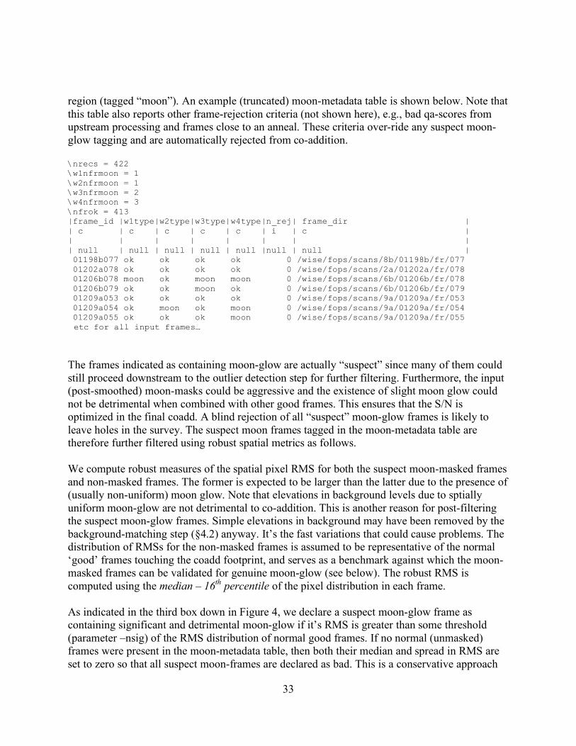
region (tagged “moon”). An example (truncated) moon-metadata table is shown below. Note that this table also reports other frame-rejection criteria (not shown here), e.g., bad qa-scores from upstream processing and frames close to an anneal. These criteria over-ride any suspect moon-glow tagging and are automatically rejected from co-addition. \nrecs = 422 \w1nfrmoon = 1 \w2nfrmoon = 1 \w3nfrmoon = 2 \w4nfrmoon = 3 \nfrok = 413 |frame_id |w1type|w2type|w3type|w4type|n_rej| frame_dir | | c | c | c | c | c | i | c | | | | | | | | | | null | null | null | null | null |null | null | 01198b077 ok ok ok ok 0 /wise/fops/scans/8b/01198b/fr/077 01202a078 ok ok ok ok 0 /wise/fops/scans/2a/01202a/fr/078 01206b078 moon ok moon moon 0 /wise/fops/scans/6b/01206b/fr/078 01206b079 ok ok moon ok 0 /wise/fops/scans/6b/01206b/fr/079 01209a053 ok ok ok ok 0 /wise/fops/scans/9a/01209a/fr/053 01209a054 ok moon ok moon 0 /wise/fops/scans/9a/01209a/fr/054 01209a055 ok ok ok moon 0 /wise/fops/scans/9a/01209a/fr/055 etc for all input frames… The frames indicated as containing moon-glow are actually “suspect” since many of them could still proceed downstream to the outlier detection step for further filtering. Furthermore, the input (post-smoothed) moon-masks could be aggressive and the existence of slight moon glow could not be detrimental when combined with other good frames. This ensures that the S/N is optimized in the final coadd. A blind rejection of all “suspect” moon-glow frames is likely to leave holes in the survey. The suspect moon frames tagged in the moon-metadata table are therefore further filtered using robust spatial metrics as follows. We compute robust measures of the spatial pixel RMS for both the suspect moon-masked frames and non-masked frames. The former is expected to be larger than the latter due to the presence of (usually non-uniform) moon glow. Note that elevations in background levels due to sptially uniform moon-glow are not detrimental to co-addition. This is another reason for post-filtering the suspect moon-glow frames. Simple elevations in background may have been removed by the background-matching step (§4.2) anyway. It’s the fast variations that could cause problems. The distribution of RMSs for the non-masked frames is assumed to be representative of the normal ‘good’ frames touching the coadd footprint, and serves as a benchmark against which the moon-masked frames can be validated for genuine moon-glow (see below). The robust RMS is computed using the median – 16th percentile of the pixel distribution in each frame. As indicated in the third box down in Figure 4, we declare a suspect moon-glow frame as containing significant and detrimental moon-glow if it’s RMS is greater than some threshold (parameter –nsig) of the RMS distribution of normal good frames. If no normal (unmasked) frames were present in the moon-metadata table, then both their median and spread in RMS are set to zero so that all suspect moon-frames are declared as bad. This is a conservative approach
34
although it rarely happens since the moon-toggling maneuver in the WISE survey causes a pile-up of frames (with ~2 – 3x increase in depth-of-coverage) whenever the moon is near and unmasked frames almost always trickle through. There are handful of cases however where all of the input frames touching a footprint fall very close to the moon warranting all of them being thrown out from further processing. Holes in the survey due to severe moon-glow are therefore inevitable. Once the genuine (or worst) moon-glow frames are identified, we build coarsely sampled depth-of-coverage map using only these frames (e.g., 100 x 100 bins). We also build a depth-of-coverage map including all frames (masked + unmasked + not rejected for other reasons upstream). We then take the ratio of the moon-only depth map to the total depth map to make a moon depth-fraction (or mdf) map. This is used in the next step to decide if the moon-depth is overall too high for the pixel-outlier rejection step downstream to operate reliably. If the mdf is too high, all the moon-glow frames (the post-filtered ‘genuine’ set) are rejected from downstream processing. If not, they proceed to the outlier rejection step for further dissemination at the pixel level. This process ensures that the coadd S/N is maximized. In general, the pixel-outlier algorithm requires that no more than ~50% of a pixel stack (after interpolation) be comprised of outliers for them to be reliably detected and rejected (for details see §7). Greater than this, then that becomes the ‘norm’ for the coadd signal and no outliers will be detected. Biases will then result in the final coadd. Therefore, 50% is the breakdown point before we can be confident that outlier rejection can deal with any remaining moon-contaminated pixels. Formally, all moon-glow frames are rejected if the mdf exceeds some threshold –mfrac (default = 0.5) over a region greater than some fraction of the footprint area –mpct (default = 0.001 or 10 mdf pixels for a 100 x 100 sampled grid). As a detail, if these thresholds are not satisfied and moon-contaminated frames do proceed to the pixel-outlier detection step, the depth in any interpolated pixel stack needs to exceed a minimum specified by parameter –odet_ns (default = 4) to have a fighting chance at being reliably detected and rejected. Note that “reliably detected” is a relative and fuzzy term since in general, the outlier detection is a noisy process when the depth-of-coverage is low to moderately low, e.g., <~ 6. To avoid throwing away many good pixels, no outlier detection whatsoever is performed if the depth is ≤ 4 (or that specified by odet_ns). Therefore, if any moon-contaminated frames are passed onto the outlier detection step (after all the above post-filtering) and the total depth is relatively low (e.g., <~ 6), it’s possible to end up with moon-contamination in a co-add. This will always be true if the depth is ≤ 4 since no outlier detection is performed as described. All moon-glow frame filenames, i.e., those tagged as suspect but retained, and those eventually rejected after post-filtering are written to a log and an output summary table. All other frame rejection types are included in this table. Suspect moon frames (but not explicitly rejected by post-filtering) are assigned the mnemonic type “moon”, while actual moon-rejects are assigned “comoon” in this table. The number of suspect-moon and moon-rejected frames are written to the FITS headers of output products. Furthermore, if the –qa switch is set, montages in JPEG format of only the moon-rejected frames are generated under the directory specified by –qadir.

35
Figure 4: processing flow for rejecting moon-contaminated frames
6 OUTLIER DETECTION AND MASKING (AWOD)
6.1 Overview The goal of outlier detection is to identify frame pixel measurements of the same location on the sky which appear inconsistent with the (bulk) remainder of the sample at that location. This assumes multiple frame exposures of the same region of sky are available. Potential outliers include cosmic rays, latents (image persistence), instrumental artifacts (including bad pixels), poorly registered frames from gross pointing errors, supernovae, asteroids, and basically anything that has moved or varied appreciably with respect to the inertial sky over the observation span of a set of overlapping frames. Outlier detection and flagging has been implemented in the AWOD module (A WISE Outlier Detector), and is executed by the framecoadder script if the –odet switch has been set. In summary, the method involves first projecting and interpolating each input frame onto a common grid with user-specified pixel scale optimized for the detector's Point Spread Function (PSF) size. The interpolation is performed using the overlap-area weighting method (analogous to using a top hat kernel). This accentuates and localizes the outliers for optimal detection (e.g., cosmic ray spikes). When all frames have been interpolated, robust estimates of the first and second moments are computed for each interpolated pixel stack j. We adopt the sample median (med), and the Median Absolute Deviation (MAD) as a proxy for the dispersion:
36
!
" j #1.4826 med pi $med pi{ }{ }, (1) where pi is the value of the ith interpolated pixel within stack j. The factor of 1.4826 is the correction necessary for consistency with the standard deviation of a Normal distribution in the large sample limit. The MAD estimator is relatively immune to the presence of outliers where it exhibits a breakdown point of 50%, i.e., more than half the measurements in a sample will need to be declared outliers before the MAD gives an arbitrarily large error. The final step involves re-projecting and re-interpolating each input pixel again, but now testing each for outlier status against other values in its stack using the pre-computed robust metrics. A pixel with value pi is declared an outlier if for given “upper” (uthres) and “lower” (lthres) tail thresholds, either of the following is satisfied:
!
pi > med pi{ } + uthres" j
pi < med pi{ }# lthres" j (2)
The uthres and lthres thresholds are specified by the –tu_odet and –tl_odet command-line inputs to framecoadder respectively. If declared an outlier, a bit is set (value specified by –m_odet) in the accompanying frame mask (listed in –msklist) for use downstream. The algorithm also includes an adaptive thresholding method in that if a pixel is likely to contain “real” signal (e.g., from a source), the upper threshold is automatically inflated by a specified amount (–r_odet) to reduce the incidence of outlier flagging at that location. To distinguish between what's real or not, we generate a background subtracted median-SNR co-add using all the input pixels. The background and local noise are computed using spatial median filtering and quantile differencing: σ ≈ q0.5 - q0.16 respectively. The idea here is that since these metrics are relatively outlier resistant, a large median pixel value in the co-add (or SNR derived therefrom) is likely to contain signal associated with a source. Therefore, when flagging outliers using Eq. 2, we also threshold on the co-add SNR (with minimum tolerable value –ts_odet) to determine if uthres should be inflated by the factor –r_odet. Details are given in §6.2.2.

37
Figure 5: one-dimensional schematic of stacking method for detecting outliers for well sampled (left) and under-sampled (right) cases. The input pixel marked “×” contains signal from a source and is in danger of being flagged when outlier detection is performed at location j in the output grid. We require typically at least five samples (overlapping pixels) in a stack for the above method to be reliable. This is because the MAD measure for σ, even though robust, can itself be noisy when the sample size is small. Simulations show that for the MAD to achieve the same accuracy as the most optimal estimator of σ for a normal distribution (i.e., the sample standard deviation), the sample size needs be ≈2.74× larger. A noisy σ will adversely affect the ability to perform reliable outlier detection. The minimum number of samples (or depth-of-coverage) above which AWOD will attempt to test for outliers can be specified by the –ns_odet parameter (default=5). This can be set to 4 as the absolute minimum, but in general, we don’t recommend going below 5 since the above method becomes severely unreliable. Another requirement to ensure good reliability is to have good sampling of the instrumental PSF, i.e., at the Nyquist rate or better. When well sampled, more detector pixels in a stack can be made to align within the span of the PSF, and any pixel variations due to PSF shape are minimized. On the other hand, a PSF which is grossly under sampled can artificially increase the scatter in a stack, with the consequence of erroneously flagging pixels containing true source signal. Figure 5 illustrates these concepts. Figure 6 shows the Reliability and Completeness of outlier detection using stacks of simulated WISE frames. The simulation contains point sources with PSF is sampled at the Nyquist rate, Poisson noise spikes, and single cosmic-ray hits (outliers). For depths of-coverage of eight or
38
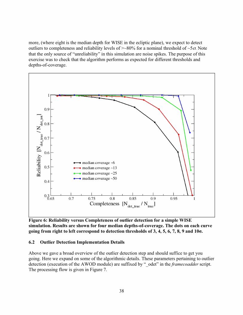
more, (where eight is the median depth for WISE in the ecliptic plane), we expect to detect outliers to completeness and reliability levels of >~80% for a nominal threshold of ~5σ. Note that the only source of “unreliability” in this simulation are noise spikes. The purpose of this exercise was to check that the algorithm performs as expected for different thresholds and depths-of-coverage.
Figure 6: Reliability versus Completeness of outlier detection for a simple WISE simulation. Results are shown for four median depths-of-coverage. The dots on each curve going from right to left correspond to detection thresholds of 3, 4, 5, 6, 7, 8, 9 and 10σ. 6.2 Outlier Detection Implementation Details Above we gave a broad overview of the outlier detection step and should suffice to get you going. Here we expand on some of the algorithmic details. These parameters pertaining to outlier detection (execution of the AWOD module) are suffixed by “_odet” in the framecoadder script. The processing flow is given in Figure 7.

39
Figure 7: Processing flow in AWOD (A WISE Outlier Detector). Red boxes represent the main computational steps
• read parameters, frame/mask lists; • initialize default parameters; • check parameter ranges, validity; • store input frame/mask filenames • store input frame WCS params;
Define WCS structure of master interpolation grid according to inputs
Define WCS positions of tiles in master grid frame if tile partitioning is requested, i.e., if Nx × Ny > 1, otherwise master grid defines a single tile.
For each of the Nx × Ny tiles:
First pass on all input frame pixels: 1. project to tile grid; 2. interpolate pixels in tile grid using overlap-area weighting; 3. store interpolated image planes that overlap with tile in a 3-D array stack; 4. compute medians of each interpolated pixel stack and robust sigma: σMAD (store these in memory).
1
Second pass on all input frame pixels: 1. re-project and re-interpolate pixels onto tile grid; 2. during process, compare interpolated values against median ± σMAD and input thresholds according to Eq. 7; 3. if outlier declared, set bit in accompanying frame mask and global mosaic-mask array; 4. enumerate outliers;
2
- report outliers to stdout and/or log file - update frame mask FITS headers with HISTORY if pixels were masked.
OUTPUTS: • 32-bit frame masks updated in-situ
(if outliers detected) with specific value 2b where b = desired bit;
• optional [-om input]: 8-bit mosaic-mask storing 0 or 1 (=> outlier detected in at least one input frame overlapping at that location);
• processing log and messages written to stdout: contains outlier enumerations and timing information;
• optional [-g]: 4 debug/diagnostic FITS files per tile: depth-of-coverage; medan co-add; σMAD image; median SNR image.
INPUTS: • list of intensity image frames; • list of accompanying masks; • master grid WCS parameters; • number of tiles along x and y; • outlier detection parameters; • output mosaic-mask filename
(optional);
40
First, the AWOD program sets up the WCS of the master interpolation grid based on the input parameters: -sizeX, -sizeY, -ra, -dec, -rot, -pa_odet, -pb_odet and other generic WCS keywords from the first listed input frame. In absolute units (projected on the sky), the master grid for outlier detection is slightly larger than the final co-add footprint by the amount “pb_odet”, where –pb_odet is an input parameter in arcsec (default=0). This parameter is additional padding for the standard footprint defined by -sizeX, -sizeY, and is recommended to be set to the PRF linear size if a PRF-interpolated co-add (or HiRes image) is desired downstream. This is because the PRF-interpolation method for co-addition will attempt to map information from outside the standard footprint from a distance equal to half the PRF size. The “–pb_odet” padding ensures that possible outliers lying just outside the desired footprint (but within the detector’s PRF size) will not introduce artifacts on the co-add (or HiRes’d image) near the boundary of the footprint. The master grid can be further partitioned into Nx × Ny tiles (via the –nx_odet and –ny_odet inputs). This is to assist with memory management when storing 3-D cubes of interpolated image frames. If tiling is desired, then each tile is assigned its own WCS with unique R.A., Dec, reference pixel coordinates, and rotation (CROTA2) equal to that of the master grid. Each tile will define a “common” interpolation grid for all input frames that overlap with it. If there is enough system memory and partitioning is not desired (i.e., Nx × Ny = 1), then the “common” tile grid is the master grid itself. For each tile (or master grid for no tiling) there are two passes through all the frame pixels [see two red boxes embedded in Figure 7]. The goal of the first pass is to compute robust (≈ outlier resistant) measures of location and spread in all interpolated pixel stacks (e.g., the median and σMAD). These products will be used in the second processing pass to actually detect and flag outliers. We outline the specifics of each step.
6.2.1 First Pass Computations The first pass projects frame pixels using a fast pixel-to-pixel WCS transformation library onto the interpolation grid. This transformation also corrects for FOV distortion using the SIP FITS representation. The interpolation uses the overlap-area weighting method to compute the flux in the output grid pixels. In essence, this method involves projecting the four corners of an input pixel directly onto the output grid (with rotation included). Input/output pixel overlap areas are then computed using a textbook algorithm for the area of a polygon, and then used as weights when summing the contribution from the pixels of an input frame with signals Di. The signal in grid pixel j from frame k is given by:
!
f jk =
aikjDik
i
"
aikji
", (3)
where aikj is the overlap area between pixel i from input frame k with output grid pixel j (see right schematic in Figure 8).
41
The projection and interpolation is only performed for those frames that overlap with the tile grid of interest. This overlap pre-filtering is performed using a coarse method whereby an overlap is declared if the separation between the centers of a tile and input frame is less than the sum of the radii of circles that circumscribe the tile and frame. The interpolated planes for each overlapping frame are stored in a 3-D cube. The median is then computed for each interpolated pixel stack j by first sorting the pixel samples using the heapsort algorithm. This uses the gsl_sort_float() routine from the GNU Scientific Library. The median is computed as the 50th percentile of the sorted stack, and we account for even numbered samples. We also compute a robust measure of the dispersion. For speed and efficiency, we use an approximation to the actual σMAD defined by Eq. 1 and call it the pseudo-MAD. This approximation works directly off a sorted array by selecting the appropriate indices. We define the pseudo-MAD as follows, where k = 0, 1, 2, 3,…N is the sample number in a sorted pixel stack, stack[k], at location j in the interpolation grid.
!
"MADj #1.482602 $1
4$ stack
3N
4
%
& ' (
) * + stack
3N
4+1
%
& ' (
) * ,
- .
/
0 1 + stack
N
4
%
& ' (
) * + stack
N
4+1
%
& ' (
) * ,
- .
/
0 1
2 3 4
5 6 7 , (4)
where the factor 1.482… is the correction to ensure Normality in the large sample limit. The array indices are rounded down to the nearest integer. The depth-of-coverage N (number of samples in a stack) must satisfy N ≥ ns_odet (default=5). If N < ns_odet, the σMADj value is set to the hard-coded “flag” value -10000 so it can be detected and avoided downstream. There is an option to smooth the σMADj image values using spatial median filtering. This is only performed if “–b_odet 1” is specified on the command-line. The default is to perform no median filtering. If requested, the window side-length of the median filter (in odd number of grid pixels) can be specified by –w_odet (default=3). The reason for smoothing the σMADj image is to avoid using erroneous (usually underestimated) values of σMADj when the depth-of-coverage is low, i.e., N <~ 10. As mentioned above, σMADj itself is not an efficient estimator of scale for small samples. Smoothing replaces each value with a median of the neighborhood, and this is expected to be more-or-less representative of the “true dispersion” in the stack at each location. If for example, the σMADj values happen to be underestimated in some regions (due to their noisy nature), this will bias flux thresholds (medj ± tσMADj ) towards low values and hence inadvertently flag “good samples” as outliers. There is also an option to scale the post-filtered σMADj values with a factor specified by –s_odet (default = 1.5). This allows the user to scale the σMADj values for each stack for consistency with expected RMS fluctuations in an image (Gaussian or otherwise). This enables one to set thresholds according to a prior measured image RMS, rather than the pseudo-MAD in pixel stacks that may be subject to under-sampling and other systematics. AWOD includes an adaptive thresholding method in that if it encounters a pixel that’s likely to be associated with a “real” signal (e.g., a source), then the upper and lower thresholds are
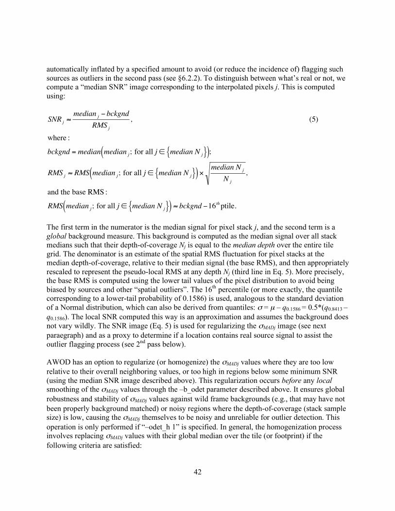
42
automatically inflated by a specified amount to avoid (or reduce the incidence of) flagging such sources as outliers in the second pass (see §6.2.2). To distinguish between what’s real or not, we compute a “median SNR” image corresponding to the interpolated pixels j. This is computed using:
!
SNR j "median j # bckgnd
RMS j
, (5)
where :
bckgnd = median median j ; for all j $ median N j{ }( );
RMS j " RMS median j ; for all j $ median N j{ }( ) %median N j
N j
,
and the base RMS :
RMS median j ; for all j $ median N j{ }( ) " bckgnd #16thptile.
The first term in the numerator is the median signal for pixel stack j, and the second term is a global background measure. This background is computed as the median signal over all stack medians such that their depth-of-coverage Nj is equal to the median depth over the entire tile grid. The denominator is an estimate of the spatial RMS fluctuation for pixel stacks at the median depth-of-coverage, relative to their median signal (the base RMS), and then appropriately rescaled to represent the pseudo-local RMS at any depth Nj (third line in Eq. 5). More precisely, the base RMS is computed using the lower tail values of the pixel distribution to avoid being biased by sources and other “spatial outliers”. The 16th percentile (or more exactly, the quantile corresponding to a lower-tail probability of 0.1586) is used, analogous to the standard deviation of a Normal distribution, which can also be derived from quantiles: σ = µ – q0.1586 = 0.5*(q0.8413 – q0.1586). The local SNR computed this way is an approximation and assumes the background does not vary wildly. The SNR image (Eq. 5) is used for regularizing the σMADj image (see next paraegraph) and as a proxy to determine if a location contains real source signal to assist the outlier flagging process (see 2nd pass below). AWOD has an option to regularize (or homogenize) the σMADj values where they are too low relative to their overall neighboring values, or too high in regions below some minimum SNR (using the median SNR image described above). This regularization occurs before any local smoothing of the σMADj values through the –b_odet parameter described above. It ensures global robustness and stability of σMADj values against wild frame backgrounds (e.g., that may have not been properly background matched) or noisy regions where the depth-of-coverage (stack sample size) is low, causing the σMADj themselves to be noisy and unreliable for outlier detection. This operation is only performed if “–odet_h 1” is specified. In general, the homogenization process involves replacing σMADj values with their global median over the tile (or footprint) if the following criteria are satisfied:

43
!
"MADj > median["MADj ] + nthres" spatial["MADj ] and SNR j # SNRmin
or
"MADj < median["MADj ]$ nthres" spatial["MADj ] regardless of SNR j
where the parameters nthres and SNRmin are the command-line inputs: –q_odet and –k_odet respectively. σspatial is a robust estimator of the global (spatial) variation in σMADj: median – 16th percentile. At the end of first pass computations, we have three image products stored in memory for a tile grid: median, pseudo-MAD (σMAD), and a SNR image. These are needed for the second pass. If the debug switch (–sdbg) is set, these three images and the depth-of-coverage map are saved to files in FITS format in the execution directory.
6.2.2 Second Pass Computations Given the robust metrics from the first pass, we now re-project (with distortion correction) and re-interpolate all the input frame pixels onto the tile grid again. The only difference here is that as each pixel from the kth input frame is projected, it is compared to the existing median, σMAD and SNR values at the same pixel location j in the tile grid to determine if it is an outlier. In general, an interpolated pixel from frame k, fjk (Eq. 3) is declared an outlier with respect to other pixels in stack j if its value satisfies:
!
f jk > median j + uthres"MADj and SNR j # SNRmin (6)
or
f jk > median j + r * uthres"MADj and SNR j > SNRmin
or
f jk < median j $ lthres"MADj and SNR j # SNRmin
or
f jk < median j $ r * lthres"MADj and SNR j > SNRmin
where the parameters uthres, lthres, r, and SNRmin correspond to the command-line inputs: –tu_odet, –tl_odet, –r_odet, and –ts_odet respectively. This is a refinement to Eq. 2. The addition here is that the upper-tail threshold, uthres is inflated by the factor r if the median SNR in pixel j exceeds some SNRmin of interest. The median is relatively immune to outliers (as long as they don’t contaminate ≥50% of the sample), therefore, if the median is relatively large, it’s likely that the pixel contains “real” source signal. The inflation factor r (–r_odet) can be set to some arbitrarily large value to avoid masking at locations where SNR > SNRmin (–ts _odet). An example where one may want to invoke this is with undersampled data (see Figure 5). If an input pixel from frame k leads to an outlier in the interpolated space of some tile, then a bit-value is set in it’s accompanying mask image. The mask value is specified by the command-line
44
input: –m_odet <2b value>, where b is the required bit. The default “–m_odet 0” means no mask updating. This could be useful if running a test to get an idea of the outlier count for threshold tuning purposes. To avoid updating (and possibly corrupting) the original input masks with outlier information, it is strongly recommended that you specify the –cpmsk command-line switch so that the original masks are copied into the local processing directory –outdir before “destructively” updating them. In addition to updating the input masks, a value “1” is also written to an output mask array at the appropriate WCS location with the same dimensions as the master interpolation grid. This is only performed if an output FITS filename: –om_odet <outfname> was specified. This product is also referred to as an outlier map in this document. This map indicates that an outlier was detected in at least one of the frame pixels in the stack at that location on the sky. Another detail in second pass processing is estimating the interpolated pixel flux fjk. This can be either done “exactly” using the area-overlap method (e.g., Eq. 3), or approximately using nearest-neighbor interpolation. The approximate method was implemented for speed, and its accuracy depends on the ratio of output-to-input pixel area, aj / ai. The value at which the nearest-neighbor method kicks in can be controlled by the –ta_odet <max out/in> parameter. This threshold represents the maximum ratio of output-to-input pixel area below which the nearest neighbor method is used. Above this threshold, the exact polygonal area-overlap method is triggered (Eq. 3). The default value for –ta_odet is 0.25, i.e., if an output pixel occupies a quarter of an input pixel or less by area (i.e., aj /ai ≤ 0.25), then the overlap will start to be appreciable (left schematic in Figure 8). The smaller this ratio, more output pixels will overlap entirely with an input pixel. In this case, the output pixel that’s nearest to the projected input pixel’s location will be assigned a signal fj ≈ (aj / ai)Di in interpolated space. If however aj /ai > 0.25, it is less likely that an input pixel will entirely overlap an output pixel (right schematic in Figure 8). In this case, all four corners of the input pixel need to be projected to compute the exact overlap area enclosed by a polygon. This is more time-consuming, but it uses less system memory in the end. If the ratio of output-to-input pixel area is >~ 0.25, then the exact overlap-area method is strongly recommended to ensure the best interpolation accuracy and representation of input pixels. Unless execution time is critical, we advise keeping “–ta_odet 0.25” (the default). If the nearest neighbor method is forced when the output/input pixel areas are really > 0.25, the variance in interpolated pixel stacks will be inflated. To compensate, you’ll need to inflate the thresholds for outlier detection (–tl_odet and –tu_odet), otherwise you may end up flagging many genuine input pixels as outliers.

45
Figure 8: Left: schematic where aout/ain <~ 0.25 with overlap area aij ≈ aout. Here the nearest neighbor to output pixel j is input pixel i. Right: schematic where aout/ain = 1 and the overlap area aij (shaded polygon) is formally computed. At the end of second pass processing, outlier pixels are enumerated per frame and reported to standard output. It’s important to note that these enumerations may contain duplicates if partitioning of the master grid into tiles was specified (i.e., with –nx_odet > 1 and/or –ny_odet > 1). This is because each tile is padded with additional pixels to avoid incomplete representation of input pixels near tile boundaries after projection. Duplicates in the reported outlier enumerations will never occur in single-tile mode (–nx 1 and –ny 1), assuming one has sufficient memory to run in this mode. In the end, the total number of outliers detected per frame can be inferred by counting the number of pixels in the mask images updated with the outlier-bit. Average and median statistics on the number of outliers detected per frame are also reported in the output QA meta-data table (–qameta <outfilename>).
6.2.3 Optimization Options The wframecoadder script includes an option to manage memory usage for outlier detection. This can be exercised by setting the “–partition” switch. Here the input image (and accompanying mask) list is partitioned if the number of input images exceeds a maximum specified by –nmaxodet. The number of tiles along x and y (–nx_odet and –ny_odet) are then reset to 1. In brief, the input image (and mask) files are first randomized to ensure the final partitioned lists contain images that more-or-less randomly (and uniformly) sample the footprint depth-of-coverage. This is because the input lists could already be ordered according to sky location for example and hence a serial partition thereof will not sample the whole footprint. Next, the optimum number of images per partition Nopt is computed by recursively halving the number of inputs Ntot until floor(Nopt) ≤ Nmax (where –nmaxodet < Nmax>) is satisfied. The input images are then segregated into “floor[(Ntot/Nopt) – 1]” sublists, each containing Nopt images. The
46
remaining “Ntot – Nopt floor[(Ntot/Nopt) – 1]” images are then added to another sublist. So for example, if Ntot = 161 and Nmax = 150, there will be two sublists, each containing 80 and 81 images. AWOD is then executed on each sublist k and outlier image maps are generated for each run in the format: <basename_sublistk.fits> where basename is read from the input specification: –om_odet <basename>. All “sublist” outlier maps are combined at the end to generate a single overall map with filename specified by –om_odet <basename>. Another feature in the outlier detection step is an option to “expand” outlier-masked pixels initially found above to ensure more complete masking of partially masked regions. This may occur from latent (image persistence) artifacts, moving objects, and/or other outlier “fuzzies” whose cores may only have been completely flagged. This post-processing is only triggered if the –expodet switch is set. The masks (residing in –outdir if –cpmsk was specified) are updated with additional outliers. The number of additional outliers is also written to standard output. The input parameters controlling this step are: –nei_odet, –nsz_odet, and –exp_odet. In brief, if a frame pixel was tagged as an outlier upstream and if a region of size “nsz_odet × nsz_odet” centered on it contains > nei_odet additional outliers (where nei_odet ≤ nsz_odet × nsz_odet), outlier expansion will be triggered around all outliers in this region. This entails blanketing “exp_odet × exp_odet” pixels around each outlier into more outliers (with bit specified by –m_odet in the mask). Figure 9 illustrates the mechanism. If the –dbg switch is set, residual FITS image masks of “new (outlier expanded) mask – input mask” are generated.

47
Figure 9: Schematic of outlier expansion method described in §6.2.3. Nout is the number of outliers initially detected within the region “nsz_odet × nsz_odet”. If this number exceeds the user-specified threshold “-nei_odet”, an additional “exp_odet × exp_odet – 1” outliers will be tagged around each pre-existing outlier. On the right is the final blanketed region for this example. Since outlier detection is the most memory intensive task, memory usage can be further reduced by invoking 2-byte integer storage and arithmetic when computing the stack estimators. This can be invoked by specifying: “–ip_odet 1” (where default = 0 ⇒ use 4-byte floating point). If specified, the floating-point values of interpolated pixels pf from each 2-D frame are transformed into the 2-byte dynamic range: -215 ≤ pi ≤ 215 – 1 (-32768 ≤ pi ≤ 32767) using a scaled log transformation:
!
pi = scale* loge[pf ], where pf > 0 and scale is a scaling factor specified by the –is_odet input parameter. This parameter has default value 2000.0 and is tuned for WISE data. For the general case, the scale factor can be tuned such that it approximately satisfies:
!
scale <32767
loge max(pf )[ ],

48
where max(pf) is the expected (approximate) maximum value of an interpolated pixel (or some percentile in the high-tail of the interpolated pixel distribution). This can be estimated from the typical maximum value of an input frame pixel multiplied by the interpolation factor: output_pixel_area/input_pixel_area ~ (pa_odet*pa_odet)/(x_scal*y_scal) where pa_odet is the pixel scale of the output interpolation grid (parameter: –pa_odet) and x_scal*y_scal is the input frame pixel area. If finding a suitable scale factor proves difficult, we suggest using the default floating-point processing (–is_odet 0).
6.2.4 Frame-based outlier rejection To further ensure coadd quality and optimize S/N, the wframecoadder script includes an option to reject entire frames from co-addition based on the number of “bad” pixels tagged upstream. The various flavors of bad pixels enumerated per frame, examples of possible causes, their default maximum tolerable numbers above which a frame will be rejected if any are exceeded, and input parameters defining these are summarized in Table 2. Note that the maximum possible thresholds are the number of pixels in each frame: 1016 x 1016 (= 1032256) pixels in w1, w2, w3 and 508 x 508 (= 258064) pixels in w4. Given that the current –tg_odet threshold (for the number of spike pixel outliers) exceeds the number of frame pixels in all bands, there is no frame rejection based on this flavor of bad pixel.
Bad pixel type searched
Examples Parameter threshold Default thresholds for w1 – w4 [#pixels]
Temporal outliers using pixel-stack statistics from AWOD. Includes spatially expanded outliers as described in §6.2.3. Note: there is no temporal outlier detection for depths-of-coverage ≤ 4
Moon glow; moving objects and heavy streaking from satellite trails; high cosmic ray count from SAA; other glitches; bad pointing solution; latents and diffraction spike smearing at high ecliptic latitudes
-tn_odet: threshold for max tolerable number of temporal outliers per frame above which entire frame will be omitted from co-addition
200000, 200000, 150000, 35000
Spike or hard-edged pixel glitches/outliers detected using median filtering in ICal pipeline. Includes hi and lo spikes. Mask bit-string param. for specifying glitch pixels is –mg_odet
Heavy cosmic-ray hit rate, e.g., from SAA; solar storms; excessive popcorn-like noise
-tg_odet: threshold for max tolerable number of spike-glitch pixels per frame above which entire frame will be omitted from co-addition
(big values => turned off) 1500000, 1500000, 1500000, 650000
Saturated pixels from saturation tagging in ICal pipeline (in any SUTR). Mask bit-string param. for
Warm transient behavior; anneals (if not explicitly filtered upstream); super-saturating sources
-tsat_odet: Threshold for max tolerable number of saturated pixels per frame above which entire frame will be omitted from co-
412000, 412000, 412000, 103000
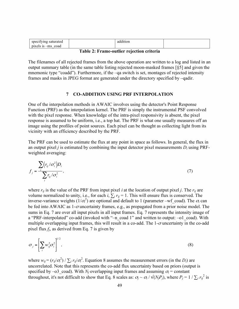
49
specifying saturated pixels is –ms_coad
addition
Table 2: Frame-outlier rejection criteria The filenames of all rejected frames from the above operation are written to a log and listed in an output summary table (in the same table listing rejected moon-masked frames [§5] and given the mnemonic type “coadd”). Furthermore, if the –qa switch is set, montages of rejected intensity frames and masks in JPEG format are generated under the directory specified by –qadir.
7 CO-ADDITION USING PRF INTERPOLATION
One of the interpolation methods in AWAIC involves using the detector's Point Response Function (PRF) as the interpolation kernel. The PRF is simply the instrumental PSF convolved with the pixel response. When knowledge of the intra-pixel responsivity is absent, the pixel response is assumed to be uniform, i.e., a top hat. The PRF is what one usually measures off an image using the profiles of point sources. Each pixel can be thought as collecting light from its vicinity with an efficiency described by the PRF. The PRF can be used to estimate the flux at any point in space as follows. In general, the flux in an output pixel j is estimated by combining the input detector pixel measurements Di using PRF-weighted averaging:
!
f j =
rij /" i
2( )Di
i
#
rij /" i
2
i
#, (7)
where rij is the value of the PRF from input pixel i at the location of output pixel j. The rij are volume normalized to unity, i.e., for each i, ∑j rij = 1. This will ensure flux is conserved. The inverse-variance weights (1/σi
2) are optional and default to 1 (parameter –wf_coad). The σi can be fed into AWAIC as 1-σ uncertainty frames, e.g., as propagated from a prior noise model. The sums in Eq. 7 are over all input pixels in all input frames. Eq. 7 represents the intensity image of a “PRF-interpolated” co-add (invoked with “–n_coad 1” and written to output: –o1_coad). With multiple overlapping input frames, this will result in a co-add. The 1-σ uncertainty in the co-add pixel flux fj, as derived from Eq. 7 is given by
!
" j = wij
2" i
2
i
#$
% &
'
( )
1/ 2
, (8)
where wij = (rij/σi
2) / ∑i rij/σi2. Equation 8 assumes the measurement errors (in the Di) are
uncorrelated. Note that this represents the co-add flux uncertainty based on priors (output is specified by –o3_coad). With Nf overlapping input frames and assuming σi = constant throughout, it's not difficult to show that Eq. 8 scales as: σj ~ σi / √(NfPj), where Pj = 1 / ∑i rij
2 is
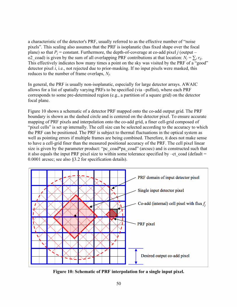
50
a characteristic of the detector's PRF, usually referred to as the effective number of “noise pixels”. This scaling also assumes that the PRF is isoplanatic (has fixed shape over the focal plane) so that Pj = constant. Furthermore, the depth-of-coverage at co-add pixel j (output –o2_coad) is given by the sum of all overlapping PRF contributions at that location: Nj = ∑i rij. This effectively indicates how many times a point on the sky was visited by the PRF of a “good” detector pixel i, i.e., not rejected due to prior-masking. If no input pixels were masked, this reduces to the number of frame overlaps, Nf. In general, the PRF is usually non-isoplanatic, especially for large detector arrays. AWAIC allows for a list of spatially varying PRFs to be specified (via –psflist), where each PRF corresponds to some pre-determined region (e.g., a partition of a square grid) on the detector focal plane. Figure 10 shows a schematic of a detector PRF mapped onto the co-add output grid. The PRF boundary is shown as the dashed circle and is centered on the detector pixel. To ensure accurate mapping of PRF pixels and interpolation onto the co-add grid, a finer cell-grid composed of “pixel cells” is set up internally. The cell size can be selected according to the accuracy to which the PRF can be positioned. The PRF is subject to thermal fluctuations in the optical system as well as pointing errors if multiple frames are being combined. Therefore, it does not make sense to have a cell-grid finer than the measured positional accuracy of the PRF. The cell pixel linear size is given by the parameter product: “pc_coad*pa_coad” (arcsec) and is constructed such that it also equals the input PRF pixel size to within some tolerance specified by –ct_coad (default = 0.0001 arcsec; see also §3.2 for specification details).
Figure 10: Schematic of PRF interpolation for a single input pixel.

51
The PRF pixels are mapped onto the cell-grid frame by first projecting the center of the detector pixel with distortion correction if necessary, and then using a local transformation with rotation to determine the positions of the PRF pixels in the cell-grid:
!
Cx
Cy
"
# $
%
& ' =
Dx
Dy
"
# $
%
& ' +
cos( )sin(
sin( cos(
"
# $
%
& ' Px ) Px
0
Py ) Py0
"
# $
%
& ' ,
where (Px, Py) is a PRF pixel coordinate, (P0
x, P0y) center-pixel coordinates of the PRF, (Dx, Dy)
are the detector pixel coordinates in the cell-grid frame, and the outputs (Cx, Cy) are the coordinates of the PRF pixel in the cell-grid frame. θ is the rotation of the input image with respect to the co-add (footprint) frame. Rotation of the input PRFs can be turned on/off using the –rf_coad option, where “–rf_coad 0” implies no rotation and we explicity set θ = 0. Turning this off can significantly speed up processing and should suffice for PRF-interpolated co-adds. For HiRes’d products however (which use the same interpolation scheme), we recommend that PRF rotation be invoked (with “–rf_coad 1”), unless of coarse the input PRFs are sufficiently axisymmetric. “Nearest-neighbor” interpolation then entails rounding the output coordinates (Cx, Cy) to the nearest integer pixel. Note that if the input PRFs are too coarsely sampled, then systematic variations may result in the output products (see §3.2 for details on how to alleviate this). The value of a PRF-weighted detector pixel flux rijDi in a co-add cell pixel j can then computed using either a nearest-neighbor match (–if _coad 0), or, an overlap-area weighting method with no rotation of input detector PRF-to-cell grid (–if _coad 1). The latter is more accurate but slower. The nearest neighbor method should suffice for most purposes. Under the overlap-area PRF-interpolation scheme (–if _coad 1), the contribution from an input PRF pixel (for a given detector pixel) is apportioned, by area, to its four neighboring cell pixels. A schematic is shown in Figure 11. Given overlap areas aijk between a PRF pixel j (from detector pixel i) and four neighboring cell pixels k of the same size, Eq. 7 for output cell pixel flux is replaced by:
!
fk =
aijkrijDi
" i
2
j
NPRF
#i
#
aijkrij
" i
2
j
NPRF
#i
# (9)
It’s important to note that the PRF transformed in this manner (regardless of interpolation method) does not use the full non-linear WCS transformation from input image to co-add frame. For large co-add footprints (linear extent >~ 16°), there could be an inaccurate representation of the PRF flux distribution towards the footprint edges - a consequence of projection off a sphere. After all the input pixels with their PRFs have been mapped, the internal co-add cells are down-sampled to the desired output co-add pixel sizes (–pa_coad).
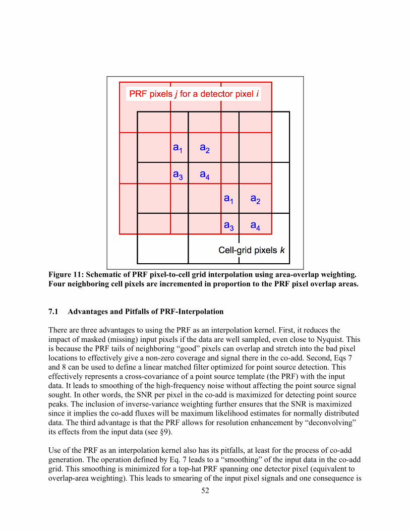
52
Figure 11: Schematic of PRF pixel-to-cell grid interpolation using area-overlap weighting. Four neighboring cell pixels are incremented in proportion to the PRF pixel overlap areas. 7.1 Advantages and Pitfalls of PRF-Interpolation There are three advantages to using the PRF as an interpolation kernel. First, it reduces the impact of masked (missing) input pixels if the data are well sampled, even close to Nyquist. This is because the PRF tails of neighboring “good” pixels can overlap and stretch into the bad pixel locations to effectively give a non-zero coverage and signal there in the co-add. Second, Eqs 7 and 8 can be used to define a linear matched filter optimized for point source detection. This effectively represents a cross-covariance of a point source template (the PRF) with the input data. It leads to smoothing of the high-frequency noise without affecting the point source signal sought. In other words, the SNR per pixel in the co-add is maximized for detecting point source peaks. The inclusion of inverse-variance weighting further ensures that the SNR is maximized since it implies the co-add fluxes will be maximum likelihood estimates for normally distributed data. The third advantage is that the PRF allows for resolution enhancement by “deconvolving” its effects from the input data (see §9). Use of the PRF as an interpolation kernel also has its pitfalls, at least for the process of co-add generation. The operation defined by Eq. 7 leads to a “smoothing” of the input data in the co-add grid. This smoothing is minimized for a top-hat PRF spanning one detector pixel (equivalent to overlap-area weighting). This leads to smearing of the input pixel signals and one consequence is

53
that cosmic rays can masquerade as point sources (albeit with narrower width) if not properly masked. For point sources with Gaussian profiles, their effective width will increase by a factor of ~√2. Furthermore, a broad kernel will cause the noise to be spatially correlated in the co-add, typically on scales (correlation lengths) approaching the PRF size. Correlations are minimized for top-hat kernels. Both the effects of flux smearing and correlated noise must be accounted for in photometric measurements off the co-add, both in profile fitting and aperture photometry. The compensation for flux smearing can be handled through an appropriate aperture correction. Ignorance of correlated noise will cause photometric uncertainties to be underestimated. Methods on how to account for correlated noise in photometry are discussed in Masci et al. (2010).
8 CO-ADDITION USING OVERLAP-AREA WEIGHTING AND DRIZZLE
Equation 7 can be compared to the popular pixel overlap-area weighting method, e.g., as implemented in the Montage1 and MOPEX2 tools. In fact if the PSF is grossly under-sampled, then the PRF is effectively a top hat spanning one detector pixel. The interpolation as described above then reduces to overlap-area weighted averaging where the interpolation weights rij become the input(i)-to-output(j) pixel overlap areas aij. AWAIC also implements the overlap-area weighting method for co-addition, in case detector PRFs are not available. This can be invoked by specifying “–sc_coad 1”. In essence, this method involves projecting the four corners of an input frame pixel directly onto the output co-add grid using the full WCS transformation with distortion correction if applicable. Input/output pixel overlap areas are computed using a formula for the area of a polygon and then used as weights when summing the contribution from all input detector pixels with signals Di. The signal in co-add pixel j (written to output: –o1_coad) is given by:
!
f j =
aij
" i
2Di
i
#
aij
" i
2
i
#, (10)
where the inverse variance weighting (1/σi
2) is optional and can be turned on/off using the –wf_coad parameter. Uncertainties based on priors, analogous to Eq. 8 are also generated (output: –o3_coad). An additional product that can only be generated for overlap-area weighting is an image of the standard-deviation of the input pixel stacks divided by the square-root of the depth-of-coverage at each location. This represents an alternative measure of the uncertainty in a co-add pixel and is generated if the –o4_coad output filename is supplied. In general, the variance in a pixel stack at location j can be written: 1 http://montage.ipac.caltech.edu/ 2 http://ssc.spitzer.caltech.edu/dataanalysistools/tools/mopex/
54
!
var j =N j
N j "1Di
2
j" Di j
2[ ], where Nj is the depth-of-coverage and the pre-factor Nj / (Nj - 1) is the correction to convert the sample variance to an unbiased estimate of the population variance. The angled brackets denote area-weighted averages of all the input detector pixel signals overlapping with co-add pixel j. The uncertainty in the co-add signal fj is then given by
!
" SDj =var j
N j
.
Using the above expressions, where <Di>j ≡ fj is given by Eq. 10, the uncertainty can be written:
!
" SDj =1
N j #1
aij
" i
2Di
2
i
$aij
" i
2
i
$# f j
2
%
&
' ' ' '
(
)
* * * *
1/ 2
. (11)
This is only computed for pixels where Nj > 1, otherwise σSDj = 0 is written to the output (–o4_coad) image. In general, estimates from Eq. 11 are expected to be larger than those estimated using priors (analogous to Eq. 8). This is because many more sources of error can contribute to the dispersion in a pixel stack, e.g., under-sampling of PSFs (even close to critical), pointing and registration errors, and temporal variations in detector/instrumental signatures. An added feature tied of the overlap-area interpolation method is a “drizzle” option, which has its roots in construction of the Hubble Deep Field images from HST3. It has the advantage of minimizing the degree of correlated noise in a co-add and can also improve the spatial resolution if the depth-of-coverage is appreciable, especially for undersampled data. Drizzling can be invoked by specifying a value 0 ≤ d < 1 for the linear drizzle factor parameter: –d_coad <d> where d = new pixel scale (or drop size) / input (native) pixel scale. I.e., the input pixel area is shrunk by a factor of d2 before proceeding with overlap-area interpolation onto the output grid (see Figure 12). This parameter has a default of 1 and implies the entire input pixels are mapped onto the output grid with no shrinkage. Note that if the drizzle factor d is too small, one may end up with holes (gaps) in the output co-add if there is insufficient depth-of-coverage. We recommend choosing a pixel drop size (d*input native scale) that is small enough to minimize degradation of the output image, but large enough that after all frames have been projected, the coverage is still fairly uniform. For
3 http://www-int.stsci.edu/~fruchter/dither/dither.html
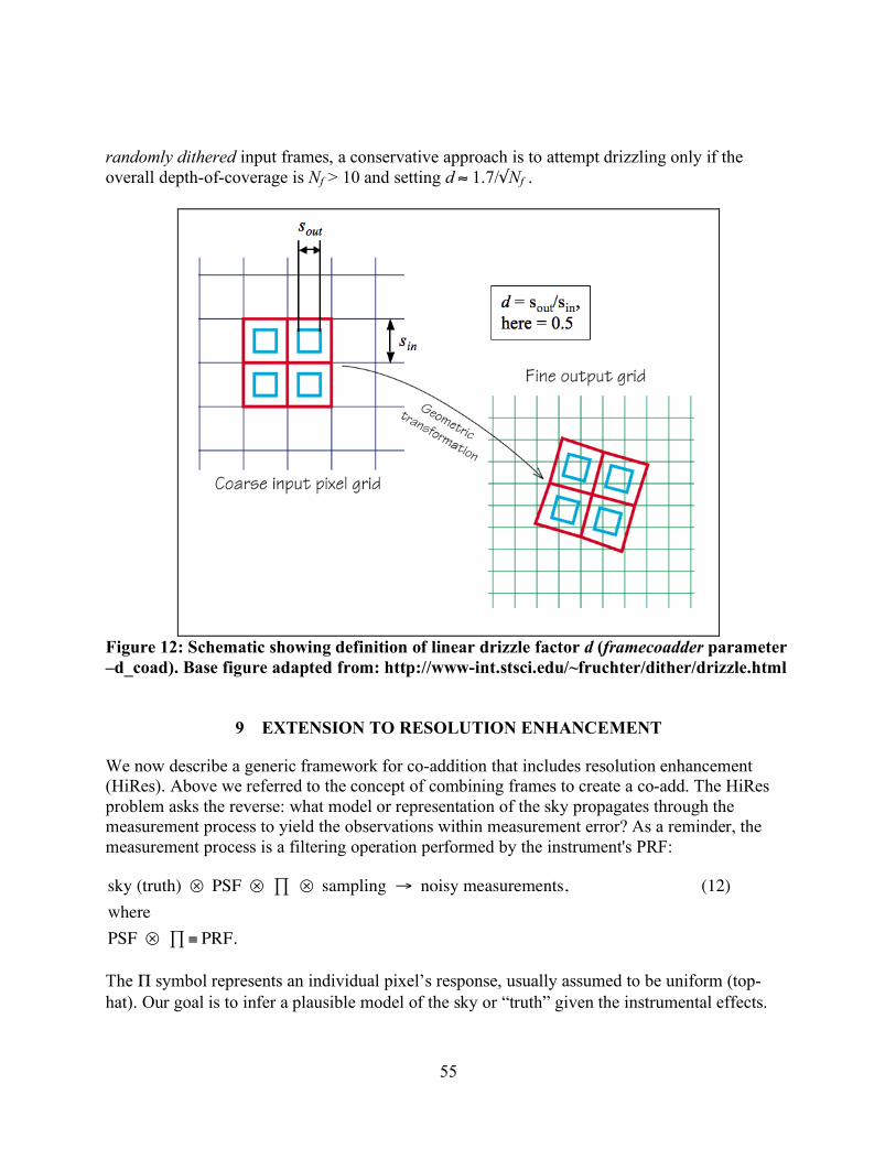
55
randomly dithered input frames, a conservative approach is to attempt drizzling only if the overall depth-of-coverage is Nf > 10 and setting d ≈ 1.7/√Nf .
Figure 12: Schematic showing definition of linear drizzle factor d (framecoadder parameter –d_coad). Base figure adapted from: http://www-int.stsci.edu/~fruchter/dither/drizzle.html
9 EXTENSION TO RESOLUTION ENHANCEMENT
We now describe a generic framework for co-addition that includes resolution enhancement (HiRes). Above we referred to the concept of combining frames to create a co-add. The HiRes problem asks the reverse: what model or representation of the sky propagates through the measurement process to yield the observations within measurement error? As a reminder, the measurement process is a filtering operation performed by the instrument's PRF:
!
sky (truth) " PSF " # " sampling $ noisy measurements, (12)
where
PSF " # % PRF.
The Π symbol represents an individual pixel’s response, usually assumed to be uniform (top-hat). Our goal is to infer a plausible model of the sky or “truth” given the instrumental effects.

56
9.1 The Maximum Correlation Method The HiRes algorithm in AWAIC is based on the Maximum Correlation Method (MCM). This was originally implemented to boost the scientific return of data from IRAS approximately 20 years ago (Aumann et al. 1990; Fowler & Aumann 1994), and is still provided as an online service to users. We have now implemented MCM in a form which is suitable for use on any imaging data that are compatible with the FITS and WCS standards, and the SIP convention for distortion. The versatility of MCM is that it implicitly generates, as its very first step (or first iteration), a PRF-interpolated co-add as described in §7. The algorithm is as follows.
1. First we begin with a flat model image of ones, i.e., a “maximally correlated” image:
!
f jn= 0
=1 " j, (13) where the subscript j refers to a pixel in the upsampled output grid, and n refers to the iteration number (input parameter –n_coad). This starting image is a first guess at the “truth” that we plan to reconstruct. Obviously this is a bad approximation, since it represents what we know without any measurements having been used yet. We could instead have used prior information as the starting model if it was available.
2. Next, we use the detector PRF(s) to “observe” this model image, or predict the input detector measurements. Starting with n = 1, the predicted flux in each detector pixel i is obtained by a “convolution”:
!
Fin
= rij f jn"1
j
# , (14)
where rij is the response (PRF value) of pixel i at the location of output model pixel j. Eq. 14 is a tensor inner product of the model image with the flipped PRF (see below for why we need to flip the PRF). It may not be a true convolution since the kernel rij may be non-isoplanatic.
3. Correction factors are computed for each detector pixel i by dividing their measured flux, Di, by those predicted from the model (Eq. 14):
!
Ki
n=Di
Fi
n. (15)
4. For each model pixel j, all “contributing” correction factors, i.e., contributed by the
overlapping PRFs of all neighboring detector pixels i are averaged using response-weighted averaging (with optional 1/σi
2 weighting):

57
!
C j
n =
rij /" i
2( )Ki
n
i
#
rij /" i
2
i
#. (16)
5. Finally, the model image pixels are multiplied by their respective averaged correction
factors (Eq. 16) to obtain new refined estimates of the model fluxes:
!
f jn
= f jn"1C j
n. (17)
If we are after a simple PRF-interpolated co-add, we terminate the process at step 5 (with output written to –o1_coad). In fact, Eq. 16 is analogous to the co-addition equation (Eq. 7) in that a starting model image with fj
0 = 1 implies a correction factor Ki1 ≡ Di since a PRF volume-
normalized to unity predicts Fi1 = 1 (Eq. 14). Therefore after the first (n = 1) iteration of MCM,
co-add fluxes will automatically result: fj1 = fj
0Cj1 = fj.
If we desire resolution enhancement, the above process is iterated, where the model image from step 5 is used to re-predict the measurements in step 2. This process of iteratively refining the model continues until the model reproduces the measurements to within the noise, i.e., the predictions from Eq. 14 are consistent with the measurements Di. If input prior uncertainties (σi) are available, this convergence can be formally checked using a global χ2 test that uses all the input detector pixels:
!
"n
2 =Di# F
i
n( )2
$i
2, (18)
i=1
N
%
where we expect χn
2 ≈ N (the number of degrees of freedom, = the number of unmasked input pixels). If input uncertainties are provided (–unclist), the reduced chi-square, χn
2/N, on a single frame basis is written to standard output following every iteration n. This is expected is converge to ≈1 as iterations increase, provided input uncertainties have been validated and adequately represent noise fluctuations in the input data. Alternatively, convergence can also be checked by examining the correction factors for each detector pixel (Eq. 15), where we expect Ki
n ≈ 1 within the noise, or, via the averaged correction factors (Eq. 16), where Cj
n → 1 after many iterations. Iterating much further beyond the initial signs of convergence has the potential of introducing unnecessary (and usually unaesthetic) detail in the model. This is important to ensure a parsimonious HiRes solution. An image of the Cj
n in the internal cell-grid frame (defined in §7) can be generated at each iteration n if –mcmprod is specified. This product is generically named “mosaic-cellcor.fits_iter<n>” and written to the directory specified by –outdir. Furthermore, the final correction-factors in the downsampled output grid (at ending iteration specified by –n_coad [n > 1]) can be written to an image specified by –o5_coad. The final HiRes’d intensity image is written to output specified by –o1_coad. For comparison/diagnostic purposes, an intensity image

58
from the first iteration (≡PRF-interpolated co-add) in the downsampled grid can be written to output specified by –of_coad. Furthermore, if –mcmprod was set, intensity images in the internal cell-grid frame at each iteration are generated under –outdir with generic name: “mosaic-cell.fits_iter<n>”. Therefore, it is an algorithmic property of MCM that it only modifies (or de-correlates) a flat starting model image to the extent necessary to make it reproduce the measurements within the noise. A PRF-interpolated co-add (from the first MCM iteration) will generally not satisfy the measurements after it is convolved with the detector PRFs, i.e., when subject to the measurement process (Eq. 12). Figure 13 shows a schematic of the MCM process.
Figure 13: Cartoon showing reconstruction of a “point source” using MCM. The process consists of iteratively refining the model using spatially dependent correction factors C (Eq. 16) such that the “convolved model” reproduces the measurements within the noise (equivalent to the C converging to unity). As a detail, the input PRFs are first flipped in x and y (or equivalently rotated by 180°) when HiRes’ing is performed (n > 1). This is to conform to the usual rules of convolution and assumes the input PRFs were made by combining images of point sources observed with the same detector in the same native x-y pixel frame. For PRF-interpolated co-adds however (that terminate at n = 1), the PRFs are not flipped since a cross-covariance with the input data is
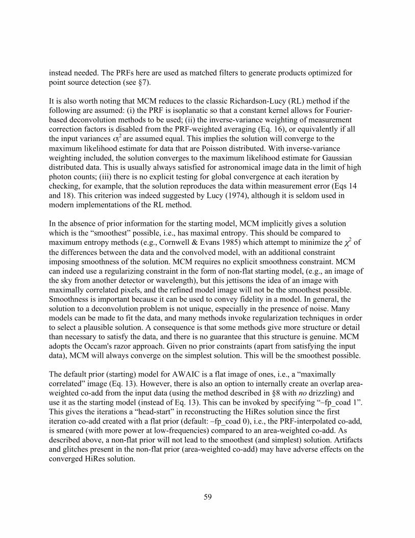
59
instead needed. The PRFs here are used as matched filters to generate products optimized for point source detection (see §7). It is also worth noting that MCM reduces to the classic Richardson-Lucy (RL) method if the following are assumed: (i) the PRF is isoplanatic so that a constant kernel allows for Fourier-based deconvolution methods to be used; (ii) the inverse-variance weighting of measurement correction factors is disabled from the PRF-weighted averaging (Eq. 16), or equivalently if all the input variances σi
2 are assumed equal. This implies the solution will converge to the maximum likelihood estimate for data that are Poisson distributed. With inverse-variance weighting included, the solution converges to the maximum likelihood estimate for Gaussian distributed data. This is usually always satisfied for astronomical image data in the limit of high photon counts; (iii) there is no explicit testing for global convergence at each iteration by checking, for example, that the solution reproduces the data within measurement error (Eqs 14 and 18). This criterion was indeed suggested by Lucy (1974), although it is seldom used in modern implementations of the RL method. In the absence of prior information for the starting model, MCM implicitly gives a solution which is the “smoothest” possible, i.e., has maximal entropy. This should be compared to maximum entropy methods (e.g., Cornwell & Evans 1985) which attempt to minimize the χ2 of the differences between the data and the convolved model, with an additional constraint imposing smoothness of the solution. MCM requires no explicit smoothness constraint. MCM can indeed use a regularizing constraint in the form of non-flat starting model, (e.g., an image of the sky from another detector or wavelength), but this jettisons the idea of an image with maximally correlated pixels, and the refined model image will not be the smoothest possible. Smoothness is important because it can be used to convey fidelity in a model. In general, the solution to a deconvolution problem is not unique, especially in the presence of noise. Many models can be made to fit the data, and many methods invoke regularization techniques in order to select a plausible solution. A consequence is that some methods give more structure or detail than necessary to satisfy the data, and there is no guarantee that this structure is genuine. MCM adopts the Occam's razor approach. Given no prior constraints (apart from satisfying the input data), MCM will always converge on the simplest solution. This will be the smoothest possible. The default prior (starting) model for AWAIC is a flat image of ones, i.e., a “maximally correlated” image (Eq. 13). However, there is also an option to internally create an overlap area-weighted co-add from the input data (using the method described in §8 with no drizzling) and use it as the starting model (instead of Eq. 13). This can be invoked by specifying “–fp_coad 1”. This gives the iterations a “head-start” in reconstructing the HiRes solution since the first iteration co-add created with a flat prior (default: –fp_coad 0), i.e., the PRF-interpolated co-add, is smeared (with more power at low-frequencies) compared to an area-weighted co-add. As described above, a non-flat prior will not lead to the smoothest (and simplest) solution. Artifacts and glitches present in the non-flat prior (area-weighted co-add) may have adverse effects on the converged HiRes solution.

60
9.2 The CFV Diagnostic A powerful diagnostic from MCM is the Correction Factor Variance (CFV). This represents the variance about the PRF-weighted average correction factor (Eq. 16) at a location in the output grid for iteration n: Vj
n = <Ki2>j – <Ki>j
2, or
!
V j
n = wij Ki
n[ ]i
"2
# wijKi
n
i
"$
% &
'
( )
2
, (19)
where wij = (rij/σi
2) / ∑i rij/σi2, and the detector-pixel correction factors Ki
n were defined in Eq. 15. At early iterations, the CFV is generally high everywhere because spatial structure has not yet been resolved, and the model contradicts the measurements when subject to the measurement process. If after convergence, all the detector-pixel measurements contributing a non-zero response at some location j agreed exactly with their predicted fluxes (Eq. 14), then all the Ki
n would be ≈ 1 and the CFV (Vj
n) at that location would be zero. Areas with a relatively large CFV indicate the presence of input pixel measurements which do not agree with the majority of the other measurements (e.g., outliers). It could also indicate noisy data, saturated data, regions where the PRF is not a good match (e.g., erroneously broad), or that a field has not yet converged and would benefit from further iteration. By thresholding the CFV, one can therefore create a mask for a HiRes image to assist in photometry, e.g., to avoid outliers and unreliable detections from amplified noise fluctuations (see below). An image of the CFV in the internal cell-grid frame (defined in §7) can be generated at each iteration n if –mcmprod is specified. This product is generically named “mosaic-cellcfv.fits_iter<n>” and written to the directory specified by –outdir. An example output from AWAIC at three iterations levels is shown in Figure 14 (this is discussed further in §9.6). Corresponding CFVs are shown in Figure 15. To illustrate the concept of the CFV, outlying input measurements were not masked in the left and middle images of Figure 15. These refer to iteration levels n = 1 and n = 40 respectively, with the latter corresponding to convergence. The smooth CFV image on the far right in Figure 15 was created from data with outliers detected and masked a priori using the algorithm described in §6. The uniformity of this CFV image indicates that the bulk of outlying measurements were indeed masked.

61
Figure 14: M51 (The Whirlpool Galaxy) from Spitzer-MIPS 24µm observations. Left: co-add (after 1 iteration); Middle: HiRes after 10 iterations; Right: HiRes after 40 iterations. Each run combined 216 frames to give a median depth-of-coverage of ~45. The fields span ~7′ × 11′.
Figure 15: Correction Factor Variance (CFV) images for M51 whose intensity images were shown in Fig. 14. For a description of the CFV, see §9.2. Left: CFV after 1 iteration with outlying measurements purposefully retained; Middle: CFV after 40 iterations with outlying measurements also purposefully retained; Right: CFV after 40 iterations but with

62
outliers masked (omitted) prior to HiRes’ing. Darkest regions correspond to lowest values of the CFV (Vj <~ 0.1), and the brightest to highest values (Vj >~ 100). 9.3 HiRes Uncertainties
9.3.1 a posteriori (data-derived) estimates Apart from providing a qualitative diagnostic, the CFV can also be used to compute a posteriori (data-derived) uncertainties in the pixel fluxes fj
n in a HiRes image. These are written to the output image filename specified by –o6_coad. In general, the 1-σ uncertainty at iteration n can be written in terms of the CFV as:
!
" j
n= c
nf jn
V j
n
riji
#, (20)
where Vj
n is the CFV defined by Eq. 19 and the sum is over the responses from all measurements i at output pixel j, i.e., the effective depth-of-coverage. cn is a correction factor to account for re distribution of noise power across spatial frequencies from one iteration to the next. At low iterations, power is relatively high at low frequencies, i.e., the noise is correlated across pixels. As iterations increase, noise is de-correlated and power migrates to high frequencies. The spectrum approaches that of white noise, provided the input measurement noise was spectrally white. Figure 16 shows the evolution of the pixel noise distribution with iteration number n using a simulation. Gaussian white noise was assumed as input. The first iteration represents the PRF-interpolated co-add where noise is maximally correlated.
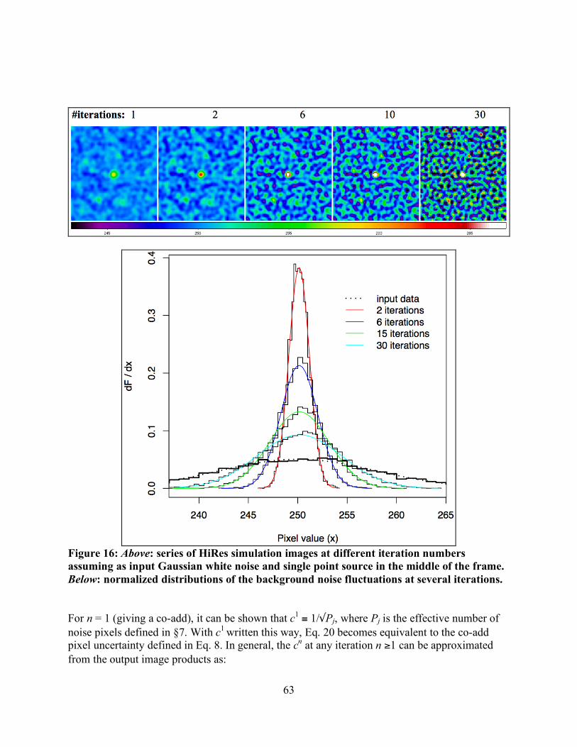
63
Figure 16: Above: series of HiRes simulation images at different iteration numbers assuming as input Gaussian white noise and single point source in the middle of the frame. Below: normalized distributions of the background noise fluctuations at several iterations. For n = 1 (giving a co-add), it can be shown that c1 ≡ 1/√Pj, where Pj is the effective number of noise pixels defined in §7. With c1 written this way, Eq. 20 becomes equivalent to the co-add pixel uncertainty defined in Eq. 8. In general, the cn at any iteration n ≥1 can be approximated from the output image products as:

64
!
cn"
#RMS f jn[ ]
# j
n[c
n =1], (21)
where σRMS is the standard-deviation (or some robust equivalent) of the pixel noise fluctuations within a “source-free” stationary background region with ≈uniform depth-of-coverage in the fj
n image. The denominator is the mean (or some robust equivalent) of Eq. 20 with cn = 1 in the same region. In AWAIC, the region for computing cn is chosen by partitioning the HiRes’d intensity image (fj
n) into a grid of –siggrid × –siggrid squares (default = 8 × 8) and then selecting the region with the smallest robust spatial RMS defined by percentiles in the pixel distribution:
!
"RMS # 0.5 p(84%tile) $ p(16%tile)[ ]. This estimate is used in the numerator of Eq. 21. It minimizes biases to the local RMS from fast-varying backgrounds, high frequency structure, and regions with high source-confusion over the footprint. If this “minimum RMS” region is still contaminated, the cn scaling factor may be overestimated (depending on how the denominator of Eq. 21 responds), leading to overestimated HiRes uncertainties from Eq. 20. This is not catastrophic since having uncertainties slightly overestimated errs on the conservative side. Furthermore, if source confusion is high everywhere, this will implicitly include confusion noise in the HiRes uncertainties. The location of the “optimal” region is written to standard output during processing and therefore we recommend visually checking the intensity image to ensure it does not contain significant structure at that location. At the time of writing, the cn uncertainty-scaling factor is always computed and applied for HiRes cases (–n_coad > 1). If you think it’s grossly wrong, then a manual rescaling of the uncertainty images (–o6_coad for CFV-derived, or –o3_coad for prior-derived; see §9.3.2 for latter) will be necessary. The above method gives pixel uncertainties which are more or less statistically compatible with background noise fluctuations in the HiRes'd image and must be interpreted with caution. This is because the background fluctuations may not be representative of the Poisson-noise where source signal is high, e.g., if the detector with which the frames were acquired is read-noise limited, it is dangerous to assume that the scaling computed above also applies at the location of sources for the purpose of estimating photometric uncertainties. The uncertainties could be slightly underestimated where the Poisson contribution is high. This may cancel out in the end if the background uncertainties were overestimated in the first place as described above. However, if the input frames are background-photon dominated (common to mid/far IR data), the HiRes uncertainties will be appropriate for all fluxes in the HiRes'd image, including at the location of sources. This will allow one to estimate uncertainties in source photometry. Note that noise correlations are also expected to be minimal in a converged HiRes image, or negligible if products were created with ringing suppression turned on (see below).

65
9.3.2 Uncertainties from propagating priors For low depths-of-coverage, estimates of the data-derived uncertainty using the CFV (Eqs 20 and 21, output: –o6_coad) may not be accurate. Even though rescaling is still involved to satisfy local RMS spatial fluctuations, there’s no guarantee that uncertainties at the location of sources will be accurate enough for photometry. An alternative estimate is written to the product specified by –o3_coad. This estimate uses the first iteration prediction using priors (Eq. 8, as applies to a PRF-interpolated co-add), and then it is rescaled using the same method described in §9.3.1 to account for the migration of noise power with increasing iteration. This assumes prior uncertainties were provided on input (–unclist) and were validated before use. In effect, the –o3_coad output product is a “pseudo-prior” uncertainty image since it uses input prior uncertainties mapped into the PRF-interpolated co-add and then rescaled to satisfy background fluctuations in the data. This product is also subject to the cautionary notes described in §9.3.1.
9.3.3 Signal-to-Noise Ratio Images There are two flavors of SNR images computed. One computed using CFV-derived 1-σ uncertainties (§9.3.1), output: –snc_coad, and another computed using pseudo-prior uncertainties (§9.3.2), output: –snu_coad. The –snu_coad can be generated for all iteration products n ≥1 (including the first iteration PRF-interpolated co-add), while the –snc_coad is only generated for HiRes products (n > 1). In either case, the SNR for output pixel j is computed using:
!
SNR j =f j " SVB j
# j
, (22)
where fj is the output HiRes or co-add image signal and SVBj is an estimate of the Slowly Varying Background at the same location. The SVB image is computed as follows: each input frame is partitioned into a grid of –svbgrid × –svbgrid squares (default = 5 × 5); each square is replaced by the median of all pixels therein; the block-median frames are then Gaussian-smoothed using a 2-D Gaussian kernel with linear extent SZ[x or y] = gausize*(NAXIS[1 or 2]/svbgrid) and sigma: σx or y = gausigm*SZ[x or y] where gausize and gausigm are input parameters: –gausize and –gausigm respectively, and NAXIS[1 or 2] are the input frame dimensions; these SVB frames are written to the working directory specified by –outdir and then co-added internally using PRF-interpolation (with masking if frame masks were specified). The output SVB co-add image is named “mosaic-int-bckgnd.fits” and generated under the –outdir directory. At the end of processing, this SVB image is used to compute the SNR images defined by Eq. 22, outputs: –snu_coad and –snc_coad for each of the σ measures described above. As a detail during the single frame SVB computations described above, if “–bmatch 1” is also specified, a search for bright/extended structure is also performed using the –ratmax (Qd) parameter described in 4.2. If detected, the frame SVB is set to a constant equal to the minimum block-median value over all –svbgrid × –svbgrid partitions. This avoids any significant structure from biasing the underlying frame background.

66
The HiRes SNR images generated here will be the maximum possible since MCM would have converged to the maximum likelihood estimate for data that were Poisson or Gaussian distributed. The latter is usually always satisfied for astronomical image data in the limit of high photon counts. In particular, the SNR image for a PRF-interpolated co-add (from output –snu_coad using “–n_coad 1”) defines a linear-matched filter optimized for point-source detection (§7.1). 9.4 Ringing Suppression Like most deconvolution methods, MCM can lead to ringing artifacts in the model image. This limits super-resolution, i.e., when attempting to go well beyond the diffraction limit of an imaging system. In general, ringing occurs because the reconstruction process tries to make the model image agree with the “true” scene with access to only the low spatial frequency components comprising the data. The input data are usually band limited, and information beyond some high spatial frequency cutoff can never be recovered. The best we can ever reconstruct is a “low-pass filtered” version of the truth, with the filter determined by the maximum spatial frequency the observations provide. This includes the finite sampling by pixels. A hard high frequency cutoff will lead to sinc-like oscillations in real image space. The magnitude of the ringing depends on the strength of a source relative to the local background intensity level. It is no accident that a solution with ringing is the smoothest (and simplest) solution possible with MCM. Anything smoother (with more low frequency power) will not satisfy the measurements when subject to the measurement process (Eq. 12). However, since a large number of less-smooth solutions can reproduce the observations, those without ringing are generally more desirable. Therefore, we relax our request for the smoothest image and use prior knowledge that the background and (desired) source fluxes are physically distinct and separable. There have been numerous approaches that have used this philosophy (e.g., Lucy 1994). A flowchart of the ringing suppression algorithm in AWAIC is shown in Figure 17. Below we expand on some of the details. Ringing suppression is only executed as part of HiRes’ing (–n_coad > 1) if the –flxbias switch was specified. See below for further tuning details.
1. We first generate an image of the slowly varying background for each input frame on some specific scale using block-median filtering over an N x N grid (–svbgrid <N>);
2. This is then subtracted from the respective input frames to create the “source” images; negative noise fluctuations are set to zero, and a tiny positive offset added;
3. MCM is then run on the background-subtracted images until convergence (with –n_coad <iterations>). This operation enforces a positivity constraint for reconstruction of the source signals. It ensures that source flux won’t ring against an essentially zero background level so power can be forced into high spatial frequencies;
4. The background images are co-added and then optionally added to the HiRes’d source-image product. This is only performed if the –addbck switch is specified. The background intensity co-add in the final downsampled grid is generically named:

67
“mosaic-int-bckgnd.fits” and written to the working directory specified by –outdir. A background intensity co-add in the internal cell-grid frame (defined in §7) is also generated and named “mosaic-cell-bckgnd.fits”.
5. After the background has been added to the HiRes’d source-only product, MCM is re-executed for several iterations (or specifically –n_coadn <iterations>) using this as the starting model image and the original frames as input. This step re-adjusts the solution and attempts to restore the intrinsic noise properties of the HiRes process, i.e., what one would have obtained if no background were removed or positivity constraint enforced. It ensures that photometric uncertainties don’t become biased and the final solution adequately reproduces the measurements within the noise.
Figure 17: ringing suppression algorithm to support HiRes
Note that ringing suppression is probably the most difficult of all components to tune in HiRes, in particular when one has extended structure covering a footprint. Here, the frame background estimates could be over-estimated, resulting in a loss of flux (and information in general) when subtracted to create the “pure-signal”, positively-constrained frames. The lost information will not participate in HiRes’ing, although it is (optionally) added back to the final HiRes’d image. This ensures flux is conserved. The goal then is to minimize SVB estimates from being contaminated from extended (and interesting) structure. This can be done by choosing a –svbgrid size such that >~50% of the pixels in each partition capture the background signal (or uninteresting parts in the frames). Some contamination is inevitable, especially for partitions which fall on top of extended structures or objects covering most of a frame’s FOV. Therefore it

68
is advised that the SVB intensity co-add (generically named –outdir/“mosaic-int-bckgnd.fits”) be examined to assess whether the partition grid size needs to be made larger (–svbgrid value smaller) or smaller (–svbgrid value larger). An example where it may need to be smaller is if one is interested in capturing the background on smaller scales so ringing can be mitigated around sources superimposed on uninteresting “fast-varying” backgrounds or structures. One can also examine the individual SVB frames corresponding to each input frame under –outdir. These have suffix: “_svb.fits”. If tweaking –svbgrid doesn’t help, there is one more functionality that can rescue the day. Along with the –flxbias switch (that triggers ringing suppression in the first place), it is recommended that the –bmatch (background matching) switch also be specified. This will assist in the explicit detection of extended structure over each frame (see §4.2) using the –ratmax threshold. If detected, it allows the frame background to default to a constant equal to the minimum median value over all –svbgrid × –svbgrid partitions of a frame (as opposed to a block-median filtered SVB). The goal here is to select the partition “most representative” of the underlying background. Depending on your extended structure or object, this may require decreasing the –ratmax threshold so that detection is triggered for your input frames (i.e., for a majority of them if you like). For super-extended structures that cover most of your input frames (or even a single frame), you may need to reduce the partition grid size (larger –svbgrid value) to try and tease out those “minimum background” regions. 9.5 Noise Suppression Algorithm A consequence of HiRes’ing is that noise-spikes at high spatial frequencies can be amplified with increasing iteration. The standard MCM algorithm does not distinguish between noise, residual outliers, and real-source information. All components are reconstructed by the deconvolution process, but not necessarily at the same rate. “Fitting of the noise” is a feature of RL-like algorithms since noise is usually present at frequencies exceeding the maximum (band-limit) of the input PRF. If a HiRes solution is to satisfy the input data on convolution with the PRF at all locations and scales, high frequency noise must persist in the HiRes image, usually with greater amplitude. One can reduce noise in the output by having a high depth-of-coverage of input frames, but high enough depths may not always be available. It is expected that the largest noise-spikes are outliers in the data and can be detected and masked by the outlier algorithm (§6) during preprocessing. This depends on the assumed outlier thresholds of course. If one is not after a science quality product (i.e., in the quantitative sense with data-compatible uncertainties), one can live dangerously and drive the outlier detection thresholds (–tl_odet and –tu_odet) really low and attempt to mask spikes well into the noise. For reliable detection, this requires a moderately high depth-of-coverage (>~15) in the first place. Again, we don’t advise attempting this unless the algorithm below cannot be tuned for your data. The noise suppression algorithm in AWAIC is still very experimental so please proceed with caution. It has been tested on the M51 case shown in Figure 14 and gives reasonable results. This makes use of the CFV diagnostic described in §9.2, in particular its change from one iteration (n) to the next (n + 1): ΔCFV. In regions of the output footprint devoid of sources and structure, and
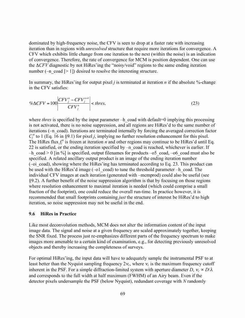
69
dominated by high-frequency noise, the CFV is seen to drop at a faster rate with increasing iteration than in regions with unresolved structure that require more iterations for convergence. A CFV which exhibits little change from one iteration to the next (within the noise) is an indication of convergence. Therefore, the rate of convergence for MCM is position dependent. One can use the ΔCFV diagnostic by not HiRes’ing the “noisy/void” regions to the same ending iteration number (–n_coad [> 1]) desired to resolve the interesting structure. In summary, the HiRes’ing for output pixel j is terminated at iteration n if the absolute %-change in the CFV satisfies:
!
%"CFV =100CFV j
n#CFVj
n+1
CFV j
n< thres, (23)
where thres is specified by the input parameter –h_coad with default=0 implying this processing is not activated, there is no noise suppression, and all regions are HiRes’d to the same number of iterations (–n_coad). Iterations are terminated internally by forcing the averaged correction factor Cj
n to 1 (Eq. 16 in §9.1) for pixel j, implying no further resolution enhancement for this pixel. The HiRes flux fj
n is frozen at iteration n and other regions may continue to be HiRes’d until Eq. 22 is satisfied, or the ending iteration specified by –n_coad is reached, whichever is earlier. If –h_coad > 0 [in %] is specified, output filenames for products –o5_coad, –o6_coad must also be specified. A related ancillary output product is an image of the ending iteration number (–oi_coad), showing where the HiRes’ing has terminated according to Eq. 23. This product can be used with the HiRes’d image (–o1_coad) to tune the threshold parameter –h_coad. The individual CFV images at each iteration (generated with –mcmprod) could also be useful (see §9.2). A further benefit of the noise suppression algorithm is that by focusing on those regions where resolution enhancement to maximal iteration is needed (which could comprise a small fraction of the footprint), one could reduce the overall run-time. In practice however, it is recommended that small footprints containing just the structure of interest be HiRes’d to high iteration, so noise suppression may not be useful in the end. 9.6 HiRes in Practice Like most deconvolution methods, MCM does not alter the information content of the input image data. The signal and noise at a given frequency are scaled approximately together, keeping the SNR fixed. The process just re-emphasizes different parts of the frequency spectrum to make images more amenable to a certain kind of examination, e.g., for detecting previously unresolved objects and thereby increasing the completeness of surveys. For optimal HiRes’ing, the input data will have to adequately sample the instrumental PSF to at least better than the Nyquist sampling frequency 2νc, where νc is the maximum frequency cutoff inherent in the PSF. For a simple diffraction-limited system with aperture diameter D, νc ∝ D/λ and corresponds to the full width at half maximum (FWHM) of an Airy beam. Even if the detector pixels undersample the PSF (below Nyquist), redundant coverage with N randomly

70
dithered frames can help recover the high spatial frequencies, since the average sampling will scale as ≈ 1/√N of an input pixel. The better the sampling, the better the HiRes algorithm is at improving spatial resolution. For imaging data from the Spitzer IRAC and MIPS detectors with typically SNR >~ 5/pixel and 10 frame overlaps, our HiRes algorithm reduces the FWHM of the effective PRF to ≈ 0.35λ/D - a factor of almost 3 below the diffraction limit. This corresponds to almost an order of magnitude increase in flux per solid angle for a Gaussian profile. This enhancement assumes accurate knowledge of the PRF over the focal plane. Example output from framecoadder at three MCM iteration levels was shown in Figure 14. At high iterations, point source ringing starts to appear. The ringing around the satellite dwarf galaxy at the bottom is aggravated because the core is saturated in the data, and the PRF used for HiRes’ing (which is derived from unsaturated data) is not a good match. “Flat” core profiles in the data, due to either saturation or improperly corrected non-linearity, will contain relatively more power in the side-lobes than the actual PRF. When this PRF is used for HiRes'ing, these side-lobes will manifest as ringing artifacts in the HiRes image in order for it to reproduce the observations on convolution with the PRF. Even though the ringing suppression algorithm was turned on in this example, ringing is still seen around other point sources. This is because these sources are superimposed on the extended structure of the galaxy. This structure acts like an elevated background against which point sources can ring. The ringing suppression algorithm relies on accurate estimation of the local background, and this can be difficult when complex structure is involved, as it is here.
10 NAN’ing LOW DEPTH-OF-COVERAGE REGIONS
Due to the unreliability of temporal (stack) outlier detection at low depths-of-coverage and its complete absence for depths ≤ 4 (or more precisely ≤ value specified by –ns_odet), the wframecoadder script has an option to replace pixels in coadd products with NaNs where the depth is less than some threshold (parameter: –cmin_coad; default = 4). This is only performed if “–crep_coad 1” is specified. At the time of writing, no low-depth pixel replacement is performed (i.e., “–crep_coad 0”). If performed, only the intensity and uncertainty co-add products have their pixels replaced by NaNs.
11 QUALITY ASSURANCE
Quality Assurance metrics are only generated if the –qa switch is specified. Below we list the output metrics for each product: intensity co-add (int); depth-of-coverage map (cov); co-add uncertainty (unc), as well as ensemble metrics for the input intensity frames (frm) and masks (msk). These are written to an output meta-data table in IPAC format (–qameta) under directory: –archdir. Below we only show the metric name and definition columns of this table. Descriptions of some of the metrics and their purpose are given below.

71
Metrics are computed for the overall footprint as well as over squares defined by an N × N grid where N is an input parameter (–qagrid <N>; default N = 3). This is to facilitate an analysis of the variation in metrics over the co-add footprint. It also provides “independent” sample sets from which to gauge the reliability of a metric (e.g., if a particular grid square happens to contain an extended source, the background-noise estimate therein will be biased). The various sigma (data-scale) measures shown below are not redundant. It is prudent to measure some of the important metrics using different methods since a specific algorithm may not be robust against unforeseen glitches and irregular behavior in the data. Each sample metric is also subject to uncertainty and bias and it's important not to be mislead by any one of them. \ QA metadata for co-add image products \ Generated by framecoadder, v.4.2 on 2010-04-13 at 13:02:28 \ Definitions of metric identifiers: \ int: co-add intensity values \ cov: depth-of-coverage map values \ unc: co-add uncertainty values \ msk: statistics on frame-pixels omitted, including temporal outliers \ frm: input frame-stack ensemble statistics \ Metric units (excluding enumerates) are in intensity co-add units \ Names appended with _xy refer to value for partition x,y in co-add footprint: e.g. for 3 x 3 grid: _11 => square at lower left corner; _33 => square at upper right \ FITS file products represented: \ 1: wise/outputs_coad1/mosaic-int.fits \ 2: wise/outputs_coad1/mosaic-cov.fits \ 3: wise/outputs_coad1/mosaic-unc.fits \ |name |comment \ \ Global co-add metrics \ coad:int:numframes Number of input frames overlapping with co-add footprint coad:int:NumNaN Number of NaN pixels over whole intensity co-add coad:unc:NumNaN Number of NaN pixels over whole uncertainty co-add coad:int:Min Minimum pixel value over whole intensity co-add coad:int:Max Maximum pixel value over whole intensity co-add coad:int:Mean Mean pixel value over whole intensity co-add coad:int:Median Median pixel value over whole intensity co-add coad:int:StdDev Standard (RMS) Deviation from mean (unbiased estimate) over co-add coad:cov:Min Minimum pixel value over whole coverage co-add coad:cov:Max Maximum pixel value over whole coverage co-add coad:cov:Mean Mean pixel value over whole coverage co-add coad:cov:Median Median pixel value over whole coverage co-add coad:cov:FivePtile 5%-tile value over whole coverage co-add coad:cov:NineFivePtile 95%-tile value over whole coverage co-add \ \ Co-add metrics for square partition 1, 1 \ coad:int:Min_11 Minimum pixel value coad:int:Max_11 Maximum pixel value coad:int:Mean_11 Mean pixel value coad:int:Median_11 Median pixel value coad:int:Mode_11 Mode pixel value (fuzzy) coad:int:StdDev_11 Standard (RMS) Deviation from mean (unbiased population estimate) coad:cov:Min_11 Minimum pixel value coad:cov:Max_11 Maximum pixel value coad:cov:Mean_11 Mean pixel value coad:cov:Median_11 Median pixel value coad:cov:FivePtile_11 5%-tile value coad:cov:NineFivePtile_11 95%-tile value coad:unc:Min_11 Minimum pixel value coad:unc:Max_11 Maximum pixel value
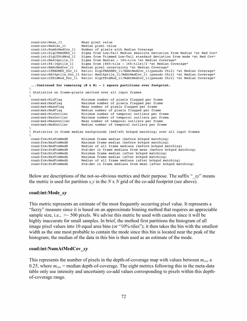
72
coad:unc:Mean_11 Mean pixel value coad:unc:Median_11 Median pixel value coad:int:NumAtMedCov_11 Number of pixels with Median Coverage coad:int:SigLTMADMED_11 Sigma from Low-Tail Median Absolute Deviation from Median *at Med Cov* coad:int:SigLTStdMod_11 Sigma from Trimmed Low-Tail standard deviation from mode *at Med Cov* coad:int:Med16ptile_11 Sigma from Median - 16%-tile *at Median Coverage* coad:int:84-16ptile_11 Sigma from [84%-tile - 16%-tile]/2 *at Median Coverage* coad:unc:MdAtMedCov_11 Median pixel uncertainty *at Median Coverage* coad:unc:LTMADMED_Unc_11 Ratio: SigLTMADMED_11/MdAtMedCov_11(pseudo Chi2) *at Median Coverage* coad:unc:Md16ptile_Unc_11 Ratio: Med16ptile_11/MdAtMedCov_11 (pseudo Chi2) *at Median Coverage* coad:unc:LTStdMod_Unc_11 Ratio: SigLTStdMod_11/MdAtMedCov_11(pseudo Chi2) *at Median Coverage* ...Continued for remaining (N x N) – 1 square partitions over footprint. \ \ Statistics on frame-pixels omitted over all input frames \ coad:msk:MinFlag Minimum number of pixels flagged per frame coad:msk:MaxFlag Maximum number of pixels flagged per frame coad:msk:MeanFlag Mean number of pixels flagged per frame coad:msk:MedFlag Median number of pixels flagged per frame coad:msk:MinOutlier Minimum number of temporal outliers per frame coad:msk:MaxOutlier Maximum number of temporal outliers per frame coad:msk:MeanOutlier Mean number of temporal outliers per frame coad:msk:MedOutlier Median number of temporal outliers per frame \ \ Statistics in frame median backgrounds (bef/aft bckgnd matching) over all input frames \ coad:frm:MinFrmMedB Minimum frame median (before bckgnd matching) coad:frm:MaxFrmMedB Maximum frame median (before bckgnd matching) coad:frm:MedFrmMedB Median of all frame medians (before bckgnd matching) coad:frm:StdFrmMedB Std-dev in frame medians from mean (before bckgnd matching) coad:frm:MinFrmMedA Minimum frame median (after bckgnd matching) coad:frm:MaxFrmMedA Maximum frame median (after bckgnd matching) coad:frm:MedFrmMedA Median of all frame medians (after bckgnd matching) coad:frm:StdFrmMedA Std-dev in frame medians from mean (after bckgnd matching)
Below are descriptions of the not-so-obvious metrics and their purpose. The suffix “_xy” means the metric is used for partition x,y in the N x N grid of the co-add footprint (see above). coad:int:Mode_xy This metric represents an estimate of the most frequently occurring pixel value. It represents a “fuzzy” measure since it is based on an approximate binning method that requires an appreciable sample size, i.e., >~ 500 pixels. We advise this metric be used with caution since it will be highly inaccurate for small samples. In brief, the method first partitions the histogram of all image pixel values into 10 equal area bins (or “10%-tiles”); it then takes the bin with the smallest width as the one most probable to contain the mode since this bin is located near the peak of the histogram; the median of the data in this bin is then used as an estimate of the mode. coad:int:NumAtMedCov_xy This represents the number of pixels in the depth-of-coverage map with values between mcov ± 0.25, where mcov = median depth-of-coverage. The eight metrics following this in the meta-data table only use intensity and uncertainty co-add values corresponding to pixels within this depth-of-coverage range.

73
coad:int:SigLTMADMED_xy This is an estimate of sigma using the Median Absolute Deviation (MAD) from the median using only pixel values in the lower tail. It is rescaled for consistency with the standard deviation of a normal distribution in the large sample limit. This measure is more robust against outliers (including sources) in the upper-tail than the sigma estimated from the sample standard deviation. Therefore it can be used to estimate the background RMS, assuming the background level is stationary. We should mention that this measure can exhibit more variation (less efficiency) than the standard-deviation on average. This metric is defined as:
!
"MAD =1.4826median pi #median{p j}{ }, where pi = the set of pixel values < sample median, pj = all pixel values in original sample. coad:int:SigLTStdMod_xy This is another robust measure of sigma that uses the mode measure above as an estimate of the first moment. It is defined as the standard-deviation of the lower-tail pixel values from the sample mode after trimming possible low-tail outliers at < 5σMAD. In other words
!
"mode =1
N #1pi #mode{p j}( )
2
i
N
$ ,
where pi = the set of pixel values in the range: mode – 5σMAD ≤ pi ≤ mode; pj = all pixels in the original sample; and σMAD was defined above. coad:int:Med16ptile_xy & coad:int:84-16ptile_xy These represent robust estimates of sigma using the sample quantile differences: ∆QL = q0.5 – q0.16 and ∆QR = 0.5(q0.84 – q0.16) respectively. For normally distributed data, these should approximately equal the standard deviation (σ). When there is severe source contamination or bright extended structure (which affects predominately the high tail), we expect ∆QR > ∆QL. coad:unc:LTMADMED_Unc_xy & coad:unc:Md16ptile_Unc_xy & coad:unc:LTStdMod_Unc_xy These represent the respective ratios:
• coad:int:SigLTMADMED_xy / coad:unc:MdAtMedCov_xy
• coad:int:Med16ptile_xy / coad:unc:MdAtMedCov_xy

74
• coad:int:SigLTStdMod_xy / coad:unc:MdAtMedCov_xy where the metrics in the numerator were defined above. The denominators contain the median uncertainty of pixels corresponding to the median depth-of-coverage (see discussion under coad:int:NumAtMedCov_xy above). These ratios can be interpreted as pseudo-χ2 measures that quantify in a broad sense, the statistical compatibility of uncertainty estimates with the distribution of co-add intensity values. In other words, whether the pixel uncertainties are compatible with the overall RMS fluctuation about the background in a co-add. If so, then these ratios should be ≈1. Even though robust sigma estimates are used, it’s important to note that high source confusion, bright extended structure, and/or a strongly varying background can make these ratios significantly deviate from 1. coad:frm:StdFrmMedB & coad:frm:StdFrmMedA These are the two most important metrics under the “Statistics in frame median backgrounds…” section of the meta-data table. They correspond to respectively the standard deviation over all the global medians of the input frames, before and after background-level matching. The before and after measures are used to assess the quality of background matching in a relative sense. The standard deviation (which quantifies the degree of scatter) is expected to be smaller after background matching. If it is not, it indicates that very little correction to the levels in the original frames was needed, or, that the presence of bright extended structure amongst frames is biasing background levels and affecting the robustness of the background-matching algorithm. 11.1 Graphics Five diagnostic plots are generated as part of the QA step. These are in SVG format and written to the directory specified by –qadir. The generic names are as follows:
• <-o1_coad>hist.svg : histogram of the co-add intensity pixel values. • <-o2_coad>hist.svg : histogram of the depth-of-coverage pixel values. • <-o1_coad>OutlierHist.svg : histogram of the number of temporal outliers (from
AWOD) detected per frame. Only generated if the –odet switch is specified. • <-o1_coad>FlaggedHist.svg : Histogram of total number of pixels flagged (omitted
from co-add) per frame as specified by the “–m_coad” masking bitstring. Only generated if the –odet switch is specified.
• <-o3_coad>VsCoverage.svg : Scatter-plot of 1-sigma uncertainty in co-add pixel flux
versus depth-of-coverage for a random sample of 5000 pixels selected over the co-add footprint. Only generated if an uncertainty product exists (was made) and the total number of pixels over footprint exceeds 5000. This plot can be used to explore the

75
scaling of uncertainty with depth-of-coverage, e.g., does it follow 1/√N statistics? If so, the points should lie on a line of slope ~ -0.5 since this is a log-log plot.
12 USAGE EXAMPLES
An example of a C-shell script for executing framecoadder to create co-adds offline in the WISE environment is: /wise/data2/fmasci/FlightAnalyses/NGC6118/awaic_coadd This is set up to make a co-add of galaxy NGC6118. The parameters are tailored to generate WISE Atlas-Image co-adds. Only parameters within the “======” delimiters need to be modified (primarily your footprint geometry and input frame lists). If you’d like make co-adds and/or HiRes’d products outside the WISE environment, e.g., on your PC, you can download and install the portable version of AWAIC from: http://wise2.ipac.caltech.edu/staff/fmasci/awaicpub.html
13 TESTING
Examples and analyses of testing can be found in the links below. The examples use data from WISE simulations, Spitzer IRAC and MIPS, and 2MASS. HiRes examples are also presented.
• Overview on AWAIC with examples: http://web.ipac.caltech.edu/staff/fmasci/home/wise/awaic.html
• Invited Talk on AWAIC: ADASS XVIII (11/04/2008, Quebec City):
http://web.ipac.caltech.edu/staff/fmasci/home/wise/adass08_talk.pdf • Paper on AWAIC (for ADASS XVIII conference):
http://web.ipac.caltech.edu/staff/fmasci/home/wise/awaic_adass08.pdf
• Example co-adds from a WSDS Processed simulation (v1.0 system release): http://web.ipac.caltech.edu/staff/fmasci/home/wise/MidLatSimMosaics2.html
• Example co-adds from 2MASS and Spitzer observations of the South Ecliptic Pole
(SEP): http://web.ipac.caltech.edu/staff/fmasci/home/wise/sep_mosaics.html • Examples/analysis from AWOD: A WISE Outlier Detector:
http://web.ipac.caltech.edu/staff/fmasci/home/wise/awod.html

76
• A Simple Background Matcher (Bmatch): http://web.ipac.caltech.edu/staff/fmasci/home/wise/bmatch.html
• Frame Co-addition Critical Design Review (01/30/2008):
http://web.ipac.caltech.edu/staff/fmasci/home/wise/Co-addition_CDRJan08.pdf
• WISE Science Team Meeting Presentation (04/19/2010): http://wise2.ipac.caltech.edu/proj/fmasci/AWAIC_STmtgApr10.pdf
14 LIENS
The following liens have been identified for the production version only. For the offline version of AWAIC, see the software description document linked on: http://wise2.ipac.caltech.edu/staff/fmasci/awaicpub.html
• Attempt to retain global background gradients (at least to first order) over coadd footprint during the frame-background matching step.
• Explore possibility of calibrating background levels on an absolute flux scale, e.g., tied to COBE. Need to maintain calibration in source-photometry.
Acknowledgments The author is indebted to the WISE team at IPAC for guidance and illuminating discussions.