Wiener Processes and Itô’s LemmaChapter 12

1

Stochastic Processes A stochastic process describes the way a variable evolves

over time that is at least in part random. i.e., temperature and IBM stock price.

A stochastic process is defined by a probability law for the evolution of a variable xt over time t. For given times, we can calculate the probability that the corresponding values x1,x2, x3,etc., lie in some specified range.

2

Categorization of Stochastic Processes

Discrete time; discrete variableRandom walk:

if can only take on discrete values Discrete time; continuous variable

is a normally distributed random variable with zero mean.

Continuous time; discrete variable Continuous time; continuous variable

ttt xx ε+= −1

ttt bxax ε++= −1

tε

3

tε

4

Modeling Stock Prices

We can use any of the four types of stochastic processes to model stock prices

The continuous time, continuous variable process proves to be the most useful for the purposes of valuing derivatives

5

Markov Processes (See pages 259-60)

In a Markov process future movements in a variable depend only on where we are, not the history of how we got where we are.

We assume that stock prices follow Markov processes.

6

Weak-Form Market Efficiency

This asserts that it is impossible to produce consistently superior returns with a trading rule based on the past history of stock prices. In other words technical analysis does not work.

A Markov process for stock prices is consistent with weak-form market efficiency

7

Example of a Discrete Time Continuous Variable Model

A stock price is currently at $40

At the end of 1 year it is considered that it will have a normal probability distribution of with mean $40 and standard deviation $10

8

Questions What is the probability distribution of the

stock price at the end of 2 years?◦ ½ years?◦ ¼ years?◦ ∆t years?

Taking limits we have defined a continuous variable, continuous time process

9

Variances & Standard Deviations

In Markov processes changes in successive periods of time are independent

This means that variances are additive Standard deviations are not additive

10

Variances & Standard Deviations (continued)

In our example it is correct to say that the variance is 100 per year.

It is strictly speaking not correct to say that the standard deviation is 10 per year.

11

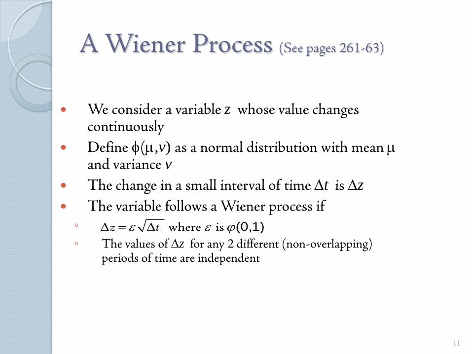
A Wiener Process (See pages 261-63)

We consider a variable z whose value changes continuously

Define φ(µ,v) as a normal distribution with mean µand variance v

The change in a small interval of time ∆t is ∆z The variable follows a Wiener process if◦◦ The values of ∆z for any 2 different (non-overlapping)

periods of time are independent

z tε ε ϕ∆ = ∆ (0,1) where is

12

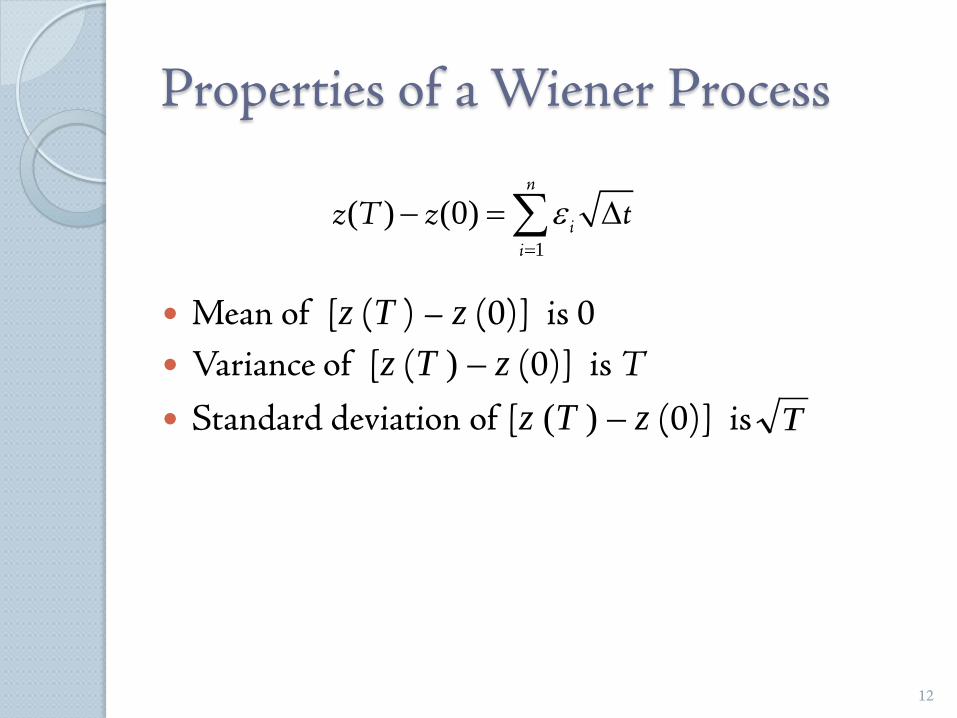
Properties of a Wiener Process

Mean of [z (T ) – z (0)] is 0 Variance of [z (T ) – z (0)] is T Standard deviation of [z (T ) – z (0)] is T

1( ) (0)

n

ii

z T z tε=

− = ∆∑

13

Taking Limits . . .

What does an expression involving dz and dtmean?

It should be interpreted as meaning that the corresponding expression involving ∆z and ∆t is true in the limit as ∆t tends to zero

In this respect, stochastic calculus is analogous to ordinary calculus

dz dtε=

14

Generalized Wiener Processes(See page 263-65)

A Wiener process has a drift rate (i.e. average change per unit time) of 0 and a variance rate of 1

In a generalized Wiener process the drift rate and the variance rate can be set equal to any chosen constants

15

Generalized Wiener Processes(continued)

The variable x follows a generalized Wiener process with a drift rate of a and a variance rate of b2 if

dx=adt+bdzor: x(t)=x0+at+bz(t)

16

Generalized Wiener Processes(continued)

Mean change in x in time T is aT Variance of change in x in time T is b2T Standard deviation of change in x in time T is b T

x a t b tε∆ = ∆ + ∆

17

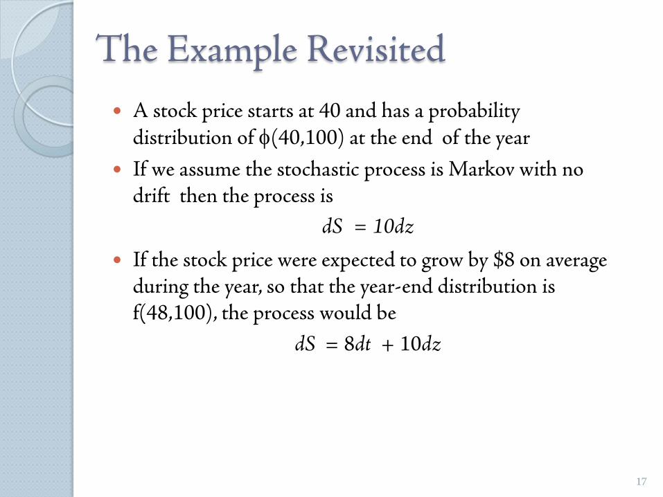
The Example Revisited A stock price starts at 40 and has a probability

distribution of φ(40,100) at the end of the year If we assume the stochastic process is Markov with no

drift then the process is dS = 10dz

If the stock price were expected to grow by $8 on average during the year, so that the year-end distribution is f(48,100), the process would be

dS = 8dt + 10dz

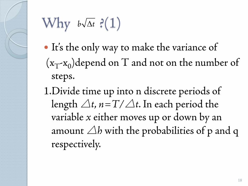
Why ?(1)

It’s the only way to make the variance of(xT-x0)depend on T and not on the number of

steps.1.Divide time up into n discrete periods of

length △t, n=T/△t. In each period the variable x either moves up or down by an amount △h with the probabilities of p and q respectively.

18

b t∆

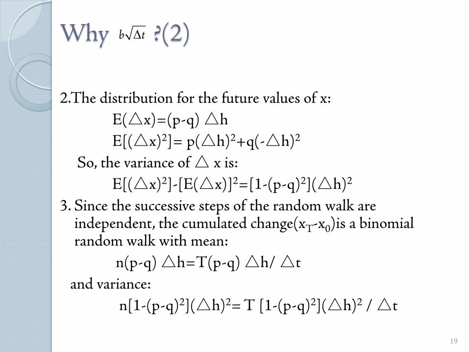
Why ?(2)

2.The distribution for the future values of x:E(△x)=(p-q) △hE[(△x)2]= p(△h)2+q(-△h)2

So, the variance of △ x is:E[(△x)2]-[E(△x)]2=[1-(p-q)2](△h)2

3. Since the successive steps of the random walk are independent, the cumulated change(xT-x0)is a binomial random walk with mean:

n(p-q) △h=T(p-q) △h/ △tand variance:

n[1-(p-q)2](△h)2= T [1-(p-q)2](△h)2 / △t

19

b t∆

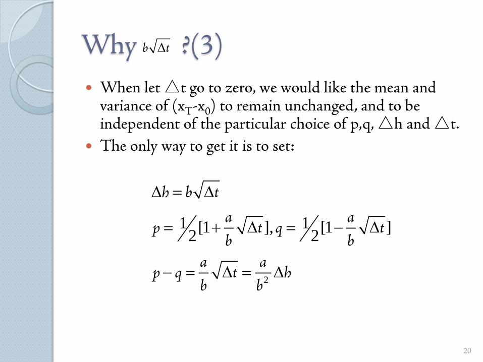
Why ?(3) When let △t go to zero, we would like the mean and

variance of (xT-x0) to remain unchanged, and to be independent of the particular choice of p,q, △h and △t.

The only way to get it is to set:

20

b t∆

2

1 1[1 ], [1 ]2 2

h b ta a

p t q tb b

a ap q t h

b b

∆ = ∆

= + ∆ = − ∆

− = ∆ = ∆

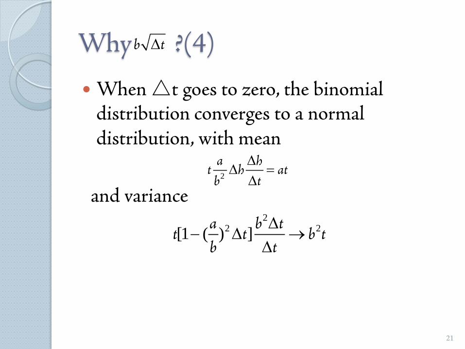
Why ?(4)

When △t goes to zero, the binomial distribution converges to a normal distribution, with mean

and variance

21

b t∆

2

a ht h atb t

∆∆ =

∆

22 2[1 ( ) ]a b t

t t b tb t

∆− ∆ →

∆

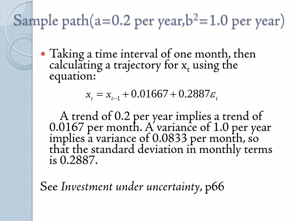
Sample path(a=0.2 per year,b2=1.0 per year)

Taking a time interval of one month, then calculating a trajectory for xt using the equation:

A trend of 0.2 per year implies a trend of 0.0167 per month. A variance of 1.0 per year implies a variance of 0.0833 per month, so that the standard deviation in monthly terms is 0.2887.

See Investment under uncertainty, p66

1 0.01667 0.2887t t tx x ε−= + +

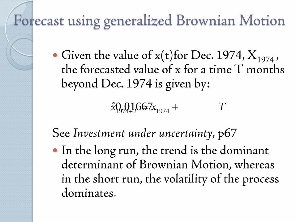
Forecast using generalized Brownian Motion

Given the value of x(t)for Dec. 1974, X1974 , the forecasted value of x for a time T months beyond Dec. 1974 is given by:

See Investment under uncertainty, p67 In the long run, the trend is the dominant

determinant of Brownian Motion, whereas in the short run, the volatility of the process dominates.

1974 1974ˆ0.01667Tx x T+ = +

24

Why a Generalized Wiener Process Is Not Appropriate for Stocks

The price of a stock never fall below zero.

For a stock price we can conjecture that its expected percentage change in a short period of time remains constant, not its expected absolute change in a short period of time

We can also conjecture that our uncertainty as to the size of future stock price movements is proportional to the level of the stock price

25

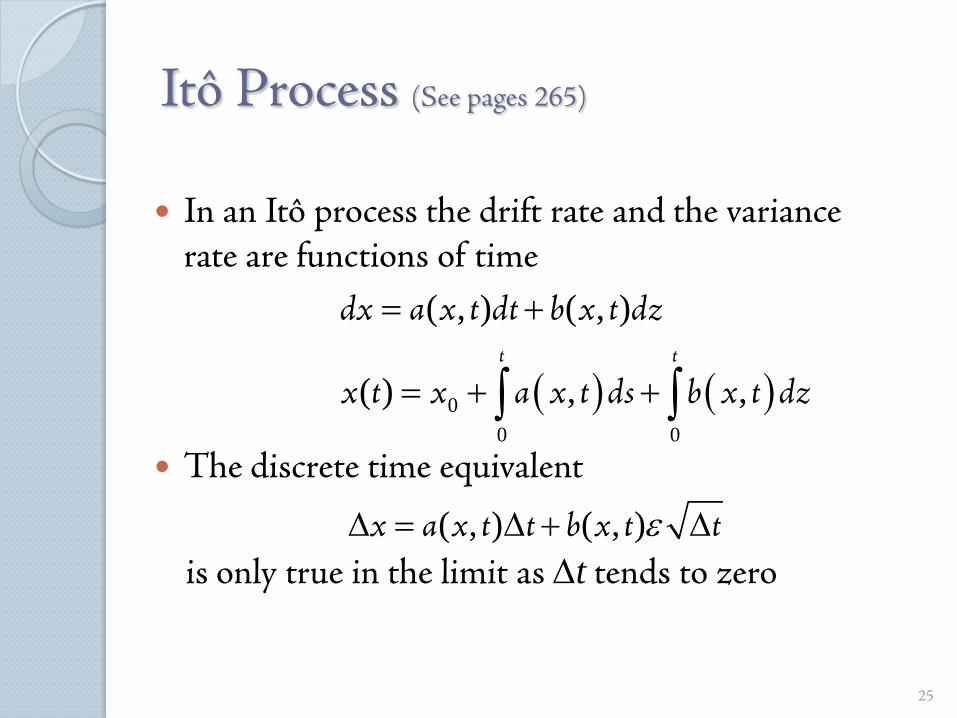
Itô Process (See pages 265)

In an Itô process the drift rate and the variance rate are functions of time

The discrete time equivalent

is only true in the limit as ∆t tends to zero( , ) ( , )x a x t t b x t tε∆ = ∆ + ∆

( ) ( )00 0

( , ) ( , )

( ) , ,t t

dx a x t dt b x t dz

x t x a x t ds b x t dz

= +

= + +∫ ∫

26

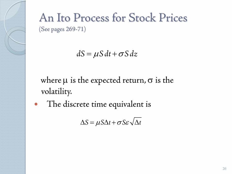
An Ito Process for Stock Prices(See pages 269-71)

where µ is the expected return, σ is the volatility.

The discrete time equivalent is

dS S dt S dzµ σ= +

S S t S tµ σ ε∆ = ∆ + ∆

27

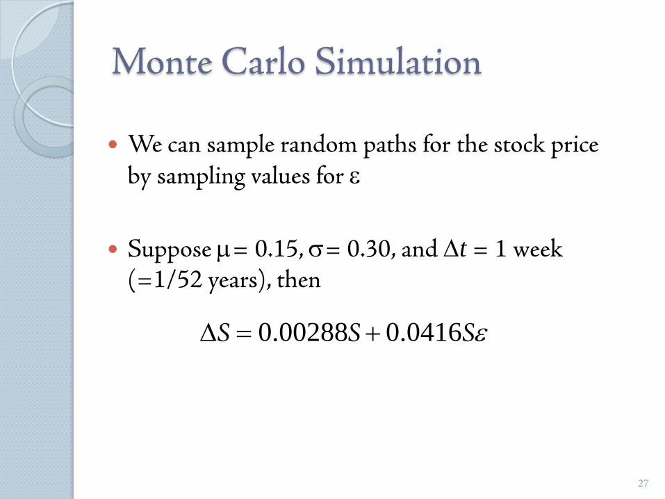
Monte Carlo Simulation

We can sample random paths for the stock price by sampling values for ε

Suppose µ= 0.15, σ= 0.30, and ∆t = 1 week (=1/52 years), then

0.00288 0.0416S S Sε∆ = +

28

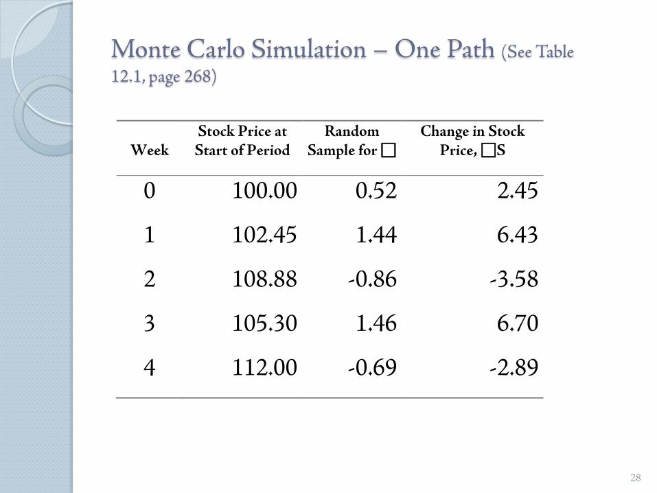
Monte Carlo Simulation – One Path (See Table 12.1, page 268)

Week

Stock Price at Start of Period

Random Sample for

Change in Stock Price, S

0 100.00 0.52 2.45

1 102.45 1.44 6.43

2 108.88 -0.86 -3.58

3 105.30 1.46 6.70

4 112.00 -0.69 -2.89

29

Itô’s Lemma (See pages 269-270)

If we know the stochastic process followed by x, Itô’s lemma tells us the stochastic process followed by some function G (x, t )

Since a derivative is a function of the price of the underlying and time, Itô’s lemma plays an important part in the analysis of derivative securities

30

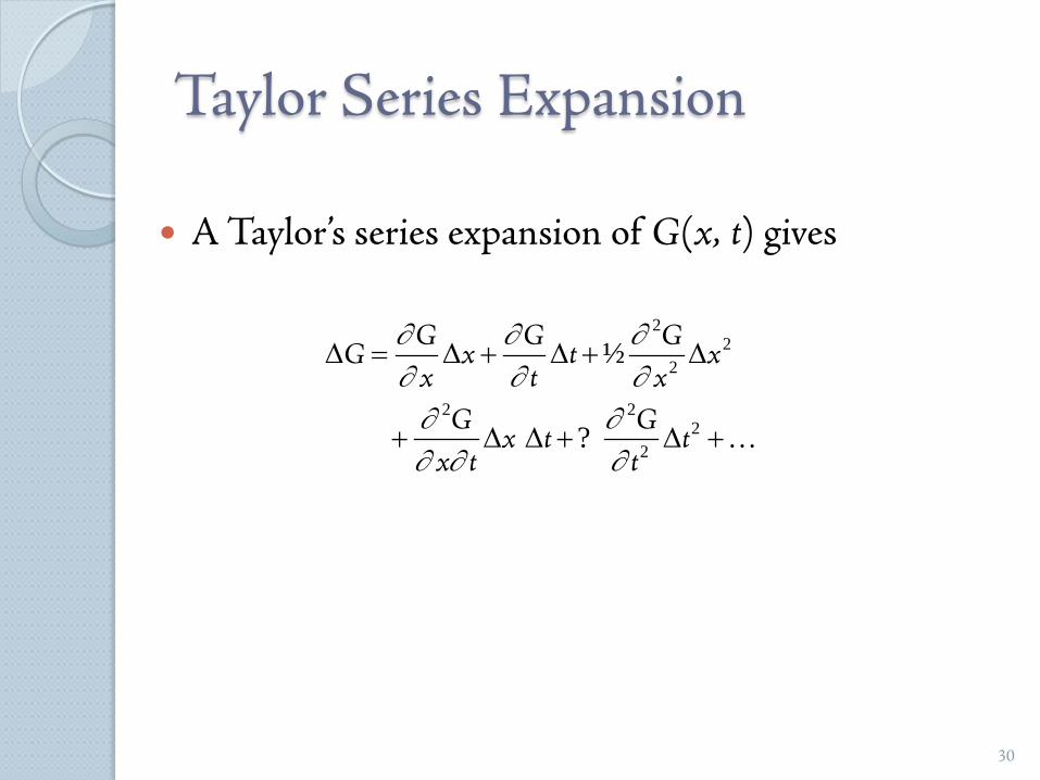
Taylor Series Expansion

A Taylor’s series expansion of G(x, t) gives

22

2

2 22

2

½

?

G G GG x t x

x t xG G

x t tx t t

∂ ∂ ∂∂ ∂ ∂∂ ∂∂ ∂ ∂

∆ = ∆ + ∆ + ∆

+ ∆ ∆ + ∆ +

31

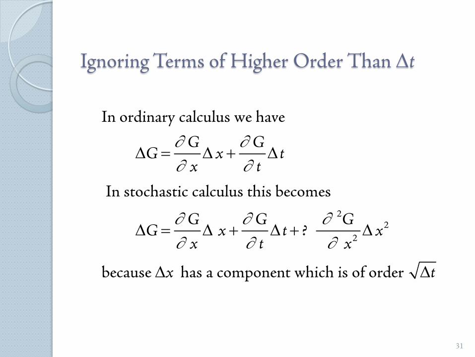
Ignoring Terms of Higher Order Than ∆t

G GG x t

x t

G G GG x t x

x t x

x t

∂ ∂∂ ∂

∂ ∂ ∂∂ ∂ ∂

∆ = ∆ + ∆

∆ = ∆ + ∆ + ∆

∆ ∆

22

2

In ordinary calculus we have

In stochastic calculus this becomes

?

because has a component which is of order

32

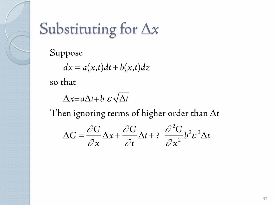
Substituting for ∆x

22 2

2

dx a x t dt b x t dz

x a t b tt

G G GG x t b t

x t x

ε

∂ ∂ ∂ ε∂ ∂ ∂

= +

∆ ∆ ∆∆

∆ = ∆ + ∆ + ∆

Suppose

( , ) ( , )

so that

= +

Then ignoring terms of higher order than

?

33

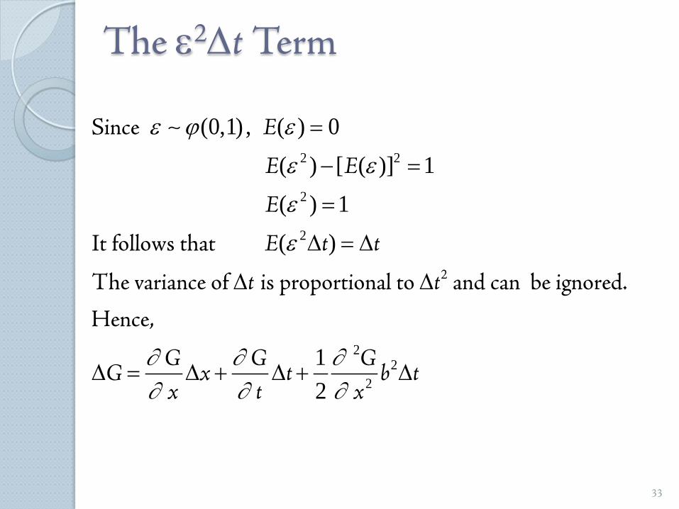
The ε2∆t Term

2 2

2

2

22

2

(0,1) , ( ) 0( ) [ ( )] 1( ) 1( )

12

E

E E

E

E t t

t t

G G GG x t b t

x t x

ε ϕ ε

ε ε

ε

ε

∂ ∂ ∂∂ ∂ ∂

=

− =

=

∆ = ∆

∆ ∆

∆ = ∆ + ∆ + ∆

2

Since

It follows that

The variance of is proportional to and can be ignored.

Hence,

34

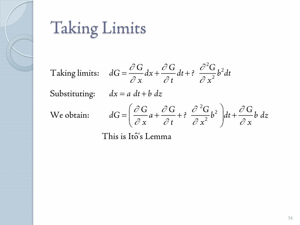
Taking Limits

22

2

22

2

ˆ

G G GdG dx dt b dt

x t xdx a dt b dz

G G G GdG a b dt b dz

x t x x

∂ ∂ ∂∂ ∂ ∂

∂ ∂ ∂ ∂∂ ∂ ∂ ∂

= + +

= +

= + + +

Taking limits: ?

Substituting:

We obtain: ?

This is Ito's Lemma

35

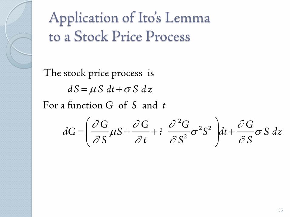
Application of Ito’s Lemmato a Stock Price Process

d S S dt S d zG S t

G G G GdG S S dt S dz

S t S S

µ σ

∂ ∂ ∂ ∂µ σ σ

∂ ∂ ∂ ∂

= +

= + + +

22 2

2

The stock price process is

For a function of and

?

36

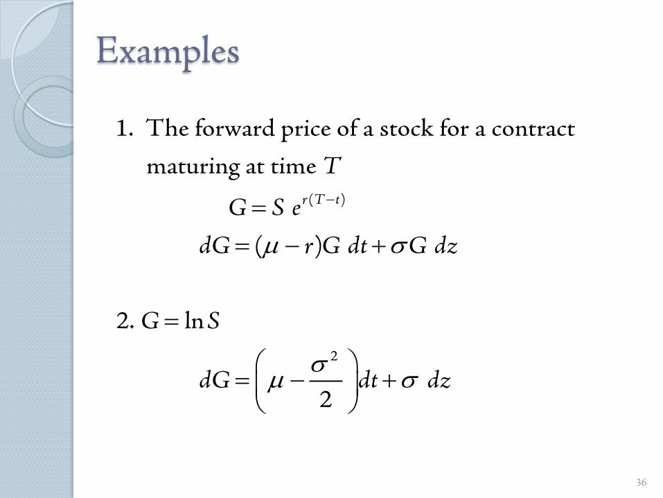
Examples

r T t

T

G S edG r G dt G dz

G S

dG dt dz

µ σ

σµ σ

−== − +

=

= − +

( )

2

1. The forward price of a stock for a contract

maturing at time

( )

2. ln

2

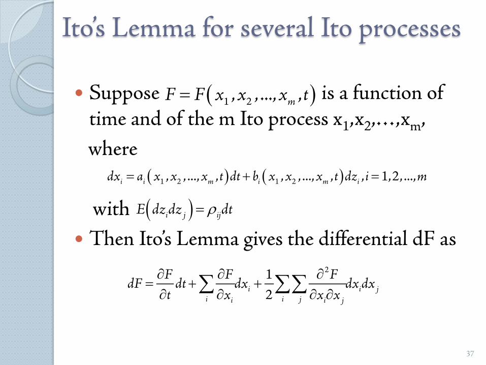
Ito’s Lemma for several Ito processes

Suppose is a function of time and of the m Ito process x1,x2,…,xm,where

with Then Ito’s Lemma gives the differential dF as

37

( ) ( )i i m i m idx a x x x t dt b x x x t dz i m= + =1 2 1 2, , ..., , , , ..., , , 1,2,...,

( )mF F x x x t= 1 2, , ..., ,

( )i j ijE dz dz dtρ=

i i ji i ji i j

F F FdF dt dx dx dx

t x x x∂ ∂ ∂

= + +∂ ∂ ∂ ∂∑ ∑∑

212

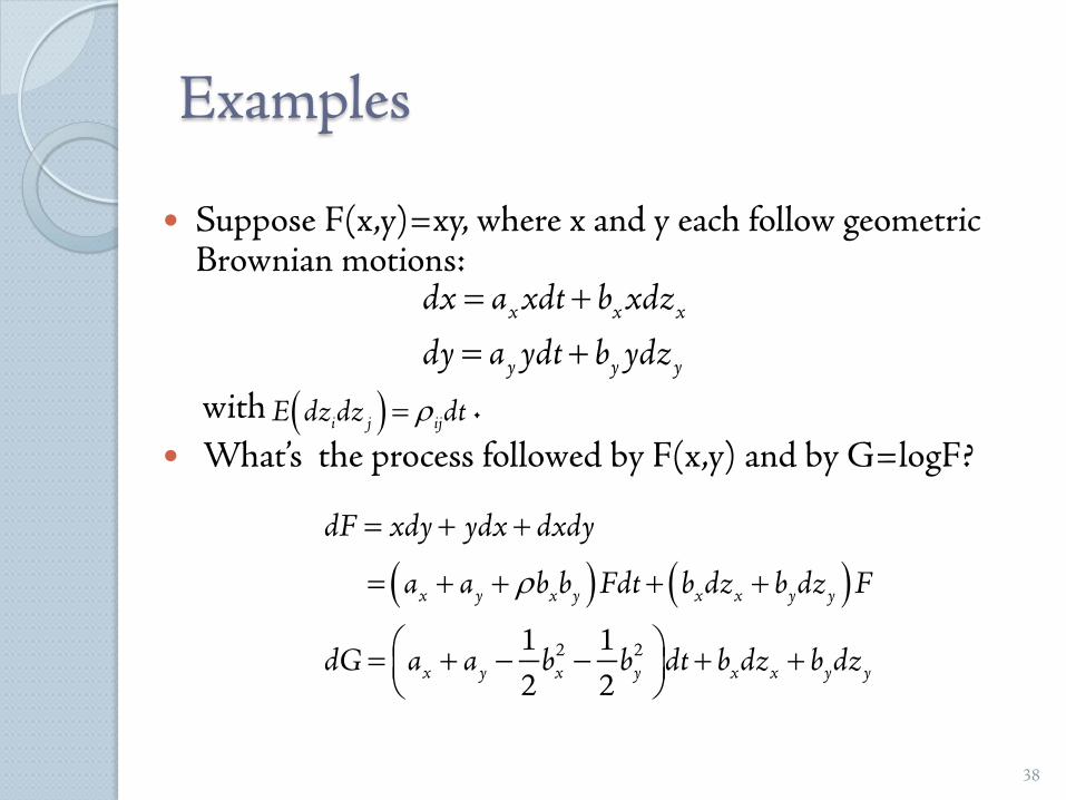
Examples

Suppose F(x,y)=xy, where x and y each follow geometric Brownian motions:

with . What’s the process followed by F(x,y) and by G=logF?

38

x x x

y y y

dx a xdt b xdzdy a ydt b ydz

= += +

( )i j ijE dz dz dtρ=

( ) ( )x y x y x x y y

x y x y x x y y

dF xdy ydx dxdy

a a b b Fdt b dz b dz F

dG a a b b dt b dz b dz

ρ

= + +

= + + + +

= + − − + +

2 21 12 2