wiener system identification using the maximum likelihood

Technical report from Automatic Control at Linköpings universitet

Wiener system identification using themaximum likelihood method

Adrian Wills, Lennart LjungDivision of Automatic ControlE-mail: [email protected], [email protected]

20th December 2010

Report no.: LiTH-ISY-R-2990Accepted for publication in Block-Oriented Nonlinear System Identifi-cation, Ed: F. Giri and E. W. Bai, Springer, 2010.

Address:Department of Electrical EngineeringLinköpings universitetSE-581 83 Linköping, Sweden

WWW: http://www.control.isy.liu.se

AUTOMATIC CONTROLREGLERTEKNIK

LINKÖPINGS UNIVERSITET

Technical reports from the Automatic Control group in Linköping are available fromhttp://www.control.isy.liu.se/publications.

http://www.control.isy.liu.se/~ljung

mailto:[email protected]

mailto:[email protected]

http://www.control.isy.liu.se/publications/?type=techreport&number=2990&go=Search&output=html

http://www.control.isy.liu.se

http://www.control.isy.liu.se/publications

Abstract

The Wiener model is a block oriented model where a linear dynamic system

block is followed by a static nonlinearity block. The dominant method to

estimate these components has been to minimize the error between the

simulated and the measured outputs. This is known to lead to biased

estimates if disturbances other than measurement noise are present. For

the case of more general disturbances we present Maximum Likelihood ex-

pressions and provide algorithms for maximising them. This includes the

case where disturbances may be coloured and as a consequence we can

handle blind estimation of Wiener models. This case is accommodated by

using the Expectation-Maximisation algorithm in combination with parti-

cles methods. Comparisons between the new algorithms and the dominant

approach con�rm that the new method is unbiased and also has superior

accuracy.

Keywords: System Identi�cation, Nonlinear models, maxximum likelihood,

Wiener models

Wiener system identification using themaximum likelihood method

Adrian Wills and Lennart Ljung

Abstract The Wiener model is a block oriented model where a linear dy-namic system block is followed by a static nonlinearity block. The dominantmethod to estimate these components has been to minimize the error be-tween the simulated and the measured outputs. This is known to lead tobiased estimates if disturbances other than measurement noise are present.For the case of more general disturbances we present Maximum Likelihoodexpressions and provide algorithms for maximising them. This includes thecase where disturbances may be coloured and as a consequence we can han-dle blind estimation of Wiener models. This case is accommodated by usingthe Expectation-Maximisation algorithm in combination with particles meth-ods. Comparisons between the new algorithms and the dominant approachconfirm that the new method is unbiased and also has superior accuracy.

Dedicated To Anna Hagenblad (1971 - 2009)

Much of the research presented in this chapter was initiated and pursued byAnna as part of her work towards a Ph.D thesis, which she sadly never had theopportunity to finish. Her interest in this research area spanned nearly ten yearsand her contributions were significant. She will be missed. We dedicate this workto the memory of Anna.

Adrian WillsSchool of Electrical Engineering and Computer Science, University of Newcastle,Callaghan, NSW, 2308, Australia e-mail: [email protected]

Lennart LjungDivision of Automatic Control, Linköpings universitet, SE-581 80 Linköping, Sweden,e-mail: [email protected]

1

2 Adrian Wills and Lennart Ljung

1 Introduction

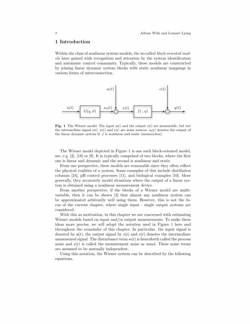
Within the class of nonlinear system models, the so-called block-oriented mod-els have gained wide recognition and attention by the system identificationand automatic control community. Typically, these models are constructedby joining linear dynamic system blocks with static nonlinear mappings invarious forms of interconnection.

u(t) x0(t)

w(t) e(t)

f(·, η)x(t) y(t)

G(q, ϑ)

Fig. 1 The Wiener model. The input u(t) and the output y(t) are measurable, but notthe intermediate signal x(t). w(t) and e(t) are noise sources. x0(t) denotes the output ofthe linear dynamic system G. f is nonlinear and static (memoryless).

The Wiener model depicted in Figure 1 is one such block-oriented model,see, e.g. [2], [18] or [9]. It is typically comprised of two blocks, where the firstone is linear and dynamic and the second is nonlinear and static.

From one perspective, these models are reasonable since they often reflectthe physical realities of a system. Some examples of this include distillationcolumns [24], pH control processes [11], and biological examples [10]. Moregenerally, they accurately model situations where the output of a linear sys-tem is obtained using a nonlinear measurement device.

From another perspective, if the blocks of a Wiener model are multi-variable, then it can be shown [3] that almost any nonlinear system canbe approximated arbitrarily well using them. However, this is not the fo-cus of the current chapter, where single input - single output systems areconsidered.

With this as motivation, in this chapter we are concerned with estimatingWiener models based on input and/or output measurements. To make theseideas more precise, we will adopt the notation used in Figure 1 here andthroughout the remainder of this chapter. In particular, the input signal isdenoted by u(t), the output signal by y(t) and x(t) denotes the intermediateunmeasured signal. The disturbance term w(t) is henceforth called the processnoise and e(t) is called the measurement noise as usual. These noise termsare assumed to be mutually independent.

Using this notation, the Wiener system can be described by the followingequations.

Wiener system identification using the maximum likelihood method 3

x0(t) = G(q,ϑ)u(t)x(t) = x0(t)+w(t)

y(t) = f(x(t),η

)+ e(t)

(1)

Throughout this chapter it is assumed that f and G each belong to aparametrized model class. Typical classes for the nonlinear term f include ba-sis function expansions such as polynomials, splines, or neural networks. Thenonlinearity f may also be a piecewise linear function, such as a dead-zoneor saturation function. Typical classes for the linear term G include rationaltransfer functions and linear state space models.

It is important to note that if the process noise w and the intermediatesignal x are unknown, then the parametrization of the Wiener model is notunique. For example, scaling the linear block G via κG and scaling the non-linear block f via f ( 1

κ·) will result in identical input–output behaviour. (It

may necessary to scale the process noise variance with a factor κ.)Based on the above description, the problem addressed in this chapter is

to estimate the parameters ϑ within the model class for G and η within themodel class for f that best match the measured output data from the system.

For convenience, we define a joint parameter vector θ as

θ = [ϑ T ,ηT ]T (2)

which will be used throughout this chapter.

2 An Output-Error Approach

While there are several methods for identifying Wiener models proposed inthe literature, the most dominant of these is to parametrize the linear and thenonlinear blocks, and then estimate the parameters from data by minimizingan output-error criterion (this has been used in [1], [21] and [22] for example).

In particular, if the process noise w(t) in Figure 1 is ignored, then a naturalcriterion is to minimize

VN(θ) =1N

N

∑t=1

(y(t)− f

(G(q,ϑ)u(t),η

))2(3)

This approach is standardly used in software packages such as [23] and [12].If it is true that the process noise w(t) is zero, then (3) becomes the

prediction-error criterion. Furthermore, if measurement noise is white andGaussian, (3) is also the Maximum Likelihood criterion and the estimate istherefore consistent [13].

Even for the case where there is process noise, it may still seem reasonableto use an output-error criterion like (3) to obtain an estimate. However,


f(G(q,ϑ)u(t),η

)is not the true predictor in this case and it has been shown

in [8] that this can result in biased estimates.A further difficulty with this approach is that is cannot directly handle the

case of blind Wiener model estimation where the process noise is assumedto be zero, but the input u(t) is not measured. Related criteria to (3) havebeen derived for this case, but they assume that the nonlinearity is invertibleand/or that the measurement noise is not present [20, 19].

By way of motivating the main tool in this chapter, namely MaximumLikelihood estimation, the next section provides conditions for the estimatesof (3) to be consistent. It is shown by example that using the output-errorcriterion can produce biased estimates. These results appeared in [8].

2.1 Consistent Estimates

Consider a Wiener system in the form of Figure 1 and Equation (1) andassume we have measurements of the input and output according to some“true” parameters (ϑ0,η0), i.e.

y(t) = f(G(q,ϑ0)u(t)+w(t),η0

)+ e(t) (4)

Based on the measured inputs and outputs, we would like to find an estimateof these parameter values, (ϑ , η) say, that are close to the true parameters. Amore precise way of describing this is to say that an estimate is consistent ifthe parameters converge to their true values as the number of data, N tendsto infinity.

In order to make this idea concrete for the output-error criterion in (3) wewrite the true system (4) as

y(t) = f(G(q,ϑ0)u(t),η0

)+ w(t)+ e(t) (5)

wherew(t) = f

(G(q,ϑ0)u(t)+w(t),η0

)− f(G(q,ϑ0)u(t),η0

)(6)

The new disturbance term w(t) may be regarded as a (input-dependent)transformation of the process noise w(t) to the output. This transformationwill most likely distort the stochastic properties of w(t), such as mean andvariance, compared with w(t).

By inserting the equation for y in (5) into the criterion (3), we receive thefollowing expression.


VN(θ) =1N

N

∑t=1

(f0− f + w(t)+ e(t)

)2(7)

=1N

N

∑t=1

(f0− f

)2+

1N

N

∑t=1

(w(t)+ e(t)

)2 +2N

N

∑t=1

(f0− f

)(w(t)+ e(t)

)where

f0 , f(G(q,ϑ0)u(t),η0

), f , f

(G(q,ϑ)u(t),η

). (8)

Further, assume that all noise terms are ergodic, so that time averages tendto their mathematical expectations as N tends to infinity. Assume also thatu is a (quasi)-stationary sequence [13], so that is also has well defined sampleaverages. Let, E denote both mathematical expectation and averaging overtime signals (cf. E in [13]). Using the fact that the measurement noise e iszero mean, and independent of the input u and the process noise w meansthat several cross terms will disappear. The criterion then tends to

V (θ) = E(

f0− f)2

+Ew2(t)+Ee2(t)+2E(

f0− f)

w(t) (9)

The last term in this expression cannot necessarily be removed since thetransformed process noise w need not be independent of u. The criterion (9)has a quadratic form, and the true values (ϑ0,η0) will minimize the criterionif and essentially only if

E(

f(G(q,ϑ0)u(t),η0

)− f(G(q,ϑ)u(t),η

))w(t) = 0 (10)

Typically, this will not hold due to the possible dependence between u andw. The parameter estimates will therefore be biased in general. To illustratethis, we provide an example below.

Example 1. Consider the following wiener system, with linear dynamic partdescribed by

x0(t)+0.5x0(t−1) = u(t−1)x(t) = x0(t)+w(t)

(11)

followed by a static nonlinearity described as a second order polynomial,

f(x(t))

= c0 + c1x2(t)

y(t) = f(x(t))+ e(t)

(12)

The goal is to estimate the nonlinearity parameters denoted here by c0 andc1.

In this case it is possible to provide expressions for the analytical minimumof criterion (3). Recall that in this case the process noise w(t) is assumed tobe zero. Therefore, the predicted output can be expressed as


y(t) = f (G(q,ϑ)u(t),η) = f (x0(t),η) = c0 + c1x20(t) (13)

Assume that all signals, noises as well as inputs, are Gaussian, zero mean andergodic. Let λx denote the variance of x0, λw denote the variance of w, andλe denote the variance of e. As N tends to infinity, the criterion (3) tends tothe limit (9)

V = E(y− y)2 = E(c0 + c1(x0 +w)2 + e− c0− c1x2

0)2

= E((c1− c1)x2

0 + c0− c0 +2c1x0w+ c1w2 + e)2

All the cross terms will be zero since the signals are Gaussian, independentand zero mean. The fourth order moments are Ex4 = 3λ 2

x and Ew4 = 3λ 2w.

This leaves

V =3(c1− c1)2λ

2x +(c0− c0)2 +4c1λxλw +3c2

1λ2w +λe

+2(c0− c0)× (c1− c1)λx +2c1(c1− c1)λxλw +2c1(c0− c0)λw

From this expression it is possible to compute the gradient with respect toeach ci and therefore find the minimum by solving

(c0− c0)+(c1− c1)+ c1λw = 0

3(c1− c1)λ 2x +(c0− c0)λx +3c1λxλw = 0

with the solution

c0 = c0 + c2λw, c1 = c1.

Therefore, the estimate of c0 is clearly biased.

Motivated by the above example, the next section investigates the use ofthe Maximum-Likelihood criterion to estimate the system parameters, whichis known to produce consistent estimates under the assumptions of this chap-ter [13].

3 The Maximum Likelihood Method

The maximum likelihood method provides estimates of the parameter valuesθ based on an observed data set YN = {y(1),y(2), . . . ,y(N)} by maximizing alikelihood function. In order to use this method it is therefore necessary tofirst derive an expression for the likelihood function itself.

The likelihood function is the probability density function (PDF) of theoutputs that is parametrized by θ . We shall assume for the moment thatthe input sequence UN = {u(1),u(2), . . . ,u(N)} is a given, deterministic se-


quence (the case of blind Wiener estimation where the input is assumed tobe stochastic is subsumed by the coloured process noise case in Section 3.2).

This likelihood will be denoted here by pθ (YN) and the Maximum-Likelihood(ML) estimate is obtained via

θ = argmaxθ

pθ (YN) (14)

This approach enjoys a long and fruitful history within the system identifi-cation community because of its statistical efficiency in producing consistentestimates (see e.g. [13]).

In the following sections we will provide expressions of the likelihood func-tion for various Wiener models. In particular, we firstly consider the systemdepicted in Figure 1 and then consider a related one whereby the processnoise is allowed to be coloured. Finally, we consider the case where the inputsignal is unknown (the is the so-called blind estimation problem).

Based on these expressions, Section 4 provides algorithms for comput-ing the ML estimate. This includes the direct gradient-based approach formodels in the form of Figure 1, which was presented in [8]. In addition,the Expectation-Maximisation approach is presented for the case of colouredprocess noise.

3.1 Likelihood Function for White Disturbances

For the Wiener model in Figure 1 we assume that the disturbance sequencese(t) and w(t) are each white noise. This means that for given input sequenceUN , y(t) will also be a sequence of independent variables. This in turn impliesthat the PDF of YN will be the product of the PDF’s of y(t), t = 1, . . . ,N.Therefore, it is sufficient to derive the PDF of y(t). To simplify notation weshall use y(t) = y, x(t) = x.

As a means to expressing this PDF, we firstly introduce an intermediatesignal x (see Figure 1) as a nuisance parameter. The benefit of introducingthis term is that the PDF of y given x is basically a reflection of the PDF ofe since y(t) = f

(x(t))+ e(t) hence

py(y|x) = pe(y− f (x,η)

)(15)

where pe is the PDF of e. In a similar manner, the PDF of x given UN canbe obtained by noting that

x(t) = G(q,ϑ)u(t)+w(t) = x0(t,ϑ)+w(t) (16)

So that for a given UN and ϑ , x0 is a known, deterministic variable, and hence

px(x) = pw(x− x0(ϑ)

)= pw

(x−G(q,ϑ)u(t)

)(17)


where pw is the PDF of w.Since x(t) is not measured, then we must integrate over all x ∈ R in order

to eliminate it from the expressions to receive

py(y) =∫

x∈Rpx,y(x,y)dx

=∫

x∈Rpy(y|x) px(x)dx

=∫

x∈Rpe(y− f (x,η)

)pw(x−G(q,ϑ)u(t)

)dx

(18)

In order to proceed further, it is necessary to assume a PDF for e and w.Therefore, we assume that the process noise w(t) and the measurement noisee(t) are Gaussian, with zero means and variances λw and λe respectively, i.e.

pe(ε)

=1√

2πλee−

12λe

ε2and pw

(v)

=1√

2πλwe−

12λw

v2(19)

The joint likelihood can be expressed as the product over all time instantssince the noise is white, so that

pθ (YN) =(

12π√

λeλw

)N N

∏t=1

∫∞

−∞

e−12 ε(t,θ)dx(t) (20)

where

ε(t,θ) =1λe

(y(t)− f

(x(t),η

))2+

1λw

(x(t)−G(q,ϑ)u(t)

)2 (21)

Therefore, when provided with the observed data UN and YN , we can calculatepθ (YN) and its gradients for each θ . This means that the ML criterion (14)can be maximized numerically. This approach is detailed in Section 4.1.

The derivation of the Likelihood function appeared in [7] and [8].

3.2 Likelihood Function for Coloured Process Noise

If the process noise is coloured, we may represent the Wiener system as inFigure 2. In this case, equations for the output are given by

x(t) = G(q,ϑ)u(t)+H(q,ϑ)w(t)

y(t) = f(x(t),η

)+ e(t)

(22)

By using the predictor form, see [13], we may write this as


u(t) x0(t)

w(t) e(t)

f(·, η)x(t) y(t)

H(q, ϑ)

G(q, ϑ)

Fig. 2 Wiener model with colored process noise. Both w(t) and e(t) are white noisesources, but w(t) is filtered through H(q,ϑ).

x(t) = x(t|Xt−1,Ut ,ϑ)+w(t) (23)x(t|Xt−1,Ut ,ϑ) , H−1(q,ϑ)G(q,ϑ)u(t)+

(1−H−1(q,ϑ)

)x(t) (24)

y(t) = f(x(t),η

)+ e(t) (25)

In the above, Xt−1 denotes the sequence Xt−1 = {x(1), . . . ,x(t−1)} and simi-larly for Ut . The only stochastic parts are e and w, hence for a given sequenceXN , the joint PDF of YN is obtained in the standard way

pYN (YN |XN) =N

∏t=1

pe(y(t)− f (x(t),η)) (26)

On the other hand, the joint PDF for XN is given by (c.f. eq (5.74), Lemma 5.1,in [13])

pXN (XN) =N

∏t=1

pw(x(t)− x(t|Xt−1,Ut ,ϑ)) (27)

The likelihood function for YN is thus obtained from (26) by integrating outthe nuisance parameter XN using its PDF (27)

pθ (YN) =∫ N

∏t=1

pw(H−1(q,ϑ)[x(t)−G(q,ϑ)u(t)]

)pe

(y(t)− f

(x(t),η

))dXN

(28)

Unfortunately, in this case filtered versions of x(t) enter the integral, whichmeans that the integration is a true multidimensional integral over the entiresequence XN . This is likely to be intractable using direct integration methodsin practise, unless the inverse noise filters are short FIR filters.

Motivated by this, here we adopt another approach whereby the noise filterH is described in state-space form as


H(q,ϑ) = C(ϑ)(qI−A(ϑ))−1B(ϑ). (29)

where A, B, C are state-space matrices, and the state update is described via

ξ (t +1) = A(ϑ)ξ (t)+B(ϑ)w(t) (30)

Therefore, according to Figure 2, the output can be expressed as

y(t) = f (C(ϑ)ξ (t)+G(q,ϑ)u(t),η)+ e(t) (31)

Equations (30) and (31) are in the form of a nonlinear state-space model,which has recently been considered in [17]. In that paper the authors use theExpectation-Maximisation algorithm in conjunction with particle methodsto compute the ML estimate. We also adopt this technique here, which isdetailed in Section 4.2.

Blind estimationNote that if the linear term G was zero, then the above system will become

a blind Wiener model, so that (31) becomes

y(t) = f (C(ϑ)ξ (t),η)+ e(t) (32)

and the parameters in H and f must be estimated via the output measure-ments only. This case is profiled via a simulation example in Section 5.3.

4 Maximum Likelihood Algorithms

For the case of white Gaussian process and measurement noise described inSection 3.1, it was mentioned that numerical methods could be used to evalu-ate the likelihood integral in Equation (20). At the same time, these methodscan be used to compute the gradient for use in a gradient based search proce-dure to find the maximum likelihood estimate. This is the approach outlinedin Section 4.1 below and profiled in Section 5 by way of simulation examples.

While this method is very useful and practical, it does not handle thecase of estimating parameters of a colouring filter for the case discussed inSection 3.2. Further, it does not handle the blind estimation case discussedin Section 3.2.

Therefore, we present an alternative method based on using the Expec-tation Maximisation (EM) approach in Section 4.2 below. A key point tonote is that this method requires a nonlinear smoothing operation and thisis achieved via particle methods. Again, the resulting algorithm is profiled inSection 5 by way of simulation studies.


4.1 Direct Gradient Based Search Approach

In this section we are concerned with maximising the likelihood functiondescribed in (20) and (21) via gradient based search. In order to avoid nu-merical conditioning issues, we consider the equivalent problem of maximisingthe log-likelihood function provided below.

θ = argmaxθ

L(θ) (33)

where

L(θ) , log(

pθ (YN))

(34)

=−N log(2π)− N2

log(λwλe)+N

∑t=1

log

(∫∞

−∞

e−12 ε(t,θ)dx

)(35)

and ε(t,θ) is given by Equation (21).To solve (33) here we employ an iterative gradient based approach. Typ-

ically, this approach proceeds by computing a “search direction”, and thenthe function L is increased along the search direction to obtain a new param-eter estimate. This search direction is usually determined so that it forms anaccute angle with the gradient, since under these conditions it can be shownto increase the cost when added to the current estimate.

To be more precise, at iteration k, L(θk) is modeled locally as

L(θk + p)≈ L(θk)+gTk p+

12

pT H−1k p, (36)

where gk is the derivative of L with respect to θ evaluated at θk and H−1k is

a symmetric matrix. If a Newton direction is desired, then H−1k would be the

inverse of Hessian matrix, but the Hessian matrix itself may be quite expen-sive to compute. However, the structure in (34) is directly amenable to usingGauss-Newton gradient based search [4], which provides a good approxima-tion to the Hessian. Here, however, we employ a quasi-Newton method whereHk is updated at each iteration based on local gradient information so thatit resembles the Hessian matrix in the limit. In particular, we use the well-known BFGS update strategy [15, Section 6.1], which can guarantee that Hkis negative definite and symmetric so that

pk =−Hkgk (37)

maximizes (36). The new parameter estimate θk+1 is then obtained by up-dating the previous one via

θk+1 = θk +αk pk, (38)


where αk is selected such that

L(θk +αk pk) > L(θk). (39)

Evaluating the cost L(θk) and its derivative gk are essential to the success ofthe above approach. For the case of computing the cost, we see from (34)that this requires the evaluation of an integral. Similarly, note that the i’thelement of the gradient vector gk, denoted gk(i), is given by

gk(i) =

N2

∂ log(λw)∂θ(i)

+N2

∂ log(λw)∂θ(i)

+12

N

∑t=1

∫∞

−∞

∂ε(t,θ)∂θ(i) e−

12 ε(t,θ)dx∫

∞

−∞e−

12 ε(t,θ)dx

∣∣∣∣∣∣θ=θk

(40)

so that computing the gradient vector also requires evaluation of an integral.Evaluating the integrals in (34) and (40) will be achieved numerically in

this chapter. In particular, we employ a fixed-interval grid over x and usethe composite Simpson’s rule to obtain the approximation [16, Chapter 4].The reason for employing a fixed grid (it need not be of fixed-interval as usedhere) is that it allows straightforward computation of L(ϑk) and its derivativegk at the same grid points. This is detailed in Algorithm 1 below and usedin the simulations in Section 5.

4.2 Expectation Maximisation Approach

In this section we address the coloured process noise case introduced in Sec-tion 3.2. As mentioned in that section, the likelihood function as expressedin (28) involved the evaluation of a high dimensional integral, which is nottractable on desktop computers. To tackle this problem, the output y(t) wasexpressed as a nonlinear state-space model via (31), (29) and (30).

In this form, the problem is directly amenable to the recently developedExpectation Maximisation (EM) algorithm described in [17]. This section willdetail the EM approach as applied to the coloured process noise case. It isalso directly applicable to the blind estimation case discussed in Section 3.2.

In keeping with the notation already defined in Section 4.1 above, theEM algorithm is a method for computing θ in (33) that is very generaland addresses a wide range of applications. Key to both its implementationand theoretical underpinnings is the consideration of a joint log-likelihoodfunction of both the measurements YN and the so-called “missing data” Z

LZ,YN (θ) = log pθ (Z,YN). (41)

In some cases, the missing data is quite literally measurements that are ab-sent for some reason. More generally though, the missing data Z consists of“measurements” that while not available, would be useful to the estimation


Algorithm 1 : Numerical computation of likelihood and derivativesGiven an odd number of grid points M, the parameter vector θ and the data UN andYN , perform the following steps. (Note that after the algorithm has terminated, the costL≈ L and gradient g≈ g).

1. Simulate the system x0(t) = G(ϑ ,q)u(t).2. Specify grid vector ∆ ∈ RM as M equidistant points between the limits [a b], so that

∆(1) = a and ∆(i+1) = ∆(i)+(b−a)/M for all i = 1, . . . ,M−1.3. Set L = N log(2π)+ N

2 log(λwλe), and g(i) = 0 for i = 1, . . . ,nθ .4. for t=1:N,

a. for j=1:M, compute

x = x0(t)+∆( j), α = x− x0(t), β = y(t)− f (x,η)

γ j = e−12 (α2/λw+β 2/λe), δ j(i) = γ j

∂ε(t,θ)∂θ(i)

, i = 1, . . . ,nθ ,

endb. Compute

κ =(b−a)

3M

γ1 +4

M−12

∑j=1

γ2 j +2

M−32

∑j=1

γ2 j+1 + γM

,

π(i) =(b−a)

3M

δ1(i)+4

M−12

∑j=1

δ2 j(i)+2

M−32

∑j=1

δ2 j+1(i)+δM(i)

, i = 1, . . . ,nθ ,

L = L− log(κ),

g(i) = g(i)+12

(∂ log(λwλe)

∂θ(i)+

π(i)κ

), i = 1, . . . ,nθ ,

end

problem. As such, the choice of Z is a design variable in the deployment ofthe EM algorithm. For the case in Section 3.2, this choice is naturally themissing state sequence

Z = {ξ1, . . . ,ξN}, (42)

since if it were known or measured, then the problem would reduce to one inthe form of (3), which is more readily soluble.

It is of vital importance to understand the connection between the jointlikelihood in (41) and the likelihood (34) that we are trying to optimise. Ac-cordingly, note that by the definition of conditional probability, the likelihood(34) and the joint likelihood (41) are related by

log pθ (YN) = log pθ (Z,YN)− log pθ (Z | YN). (43)


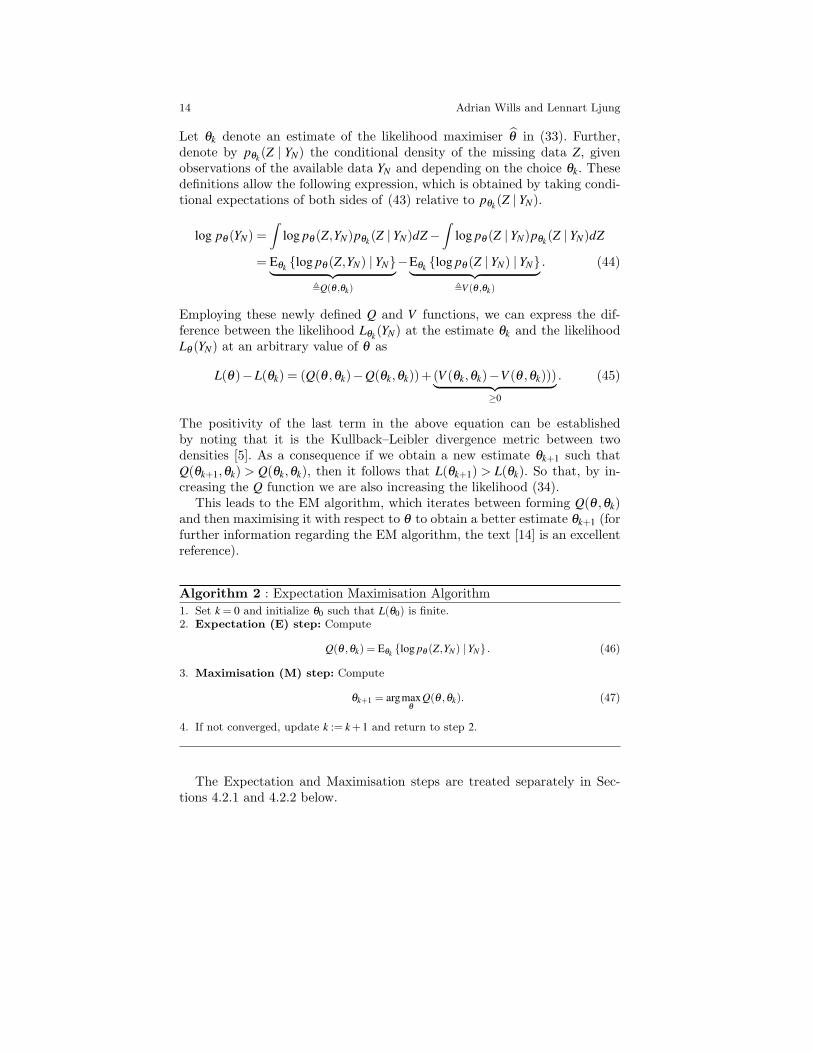
Let θk denote an estimate of the likelihood maximiser θ in (33). Further,denote by pθk(Z | YN) the conditional density of the missing data Z, givenobservations of the available data YN and depending on the choice θk. Thesedefinitions allow the following expression, which is obtained by taking condi-tional expectations of both sides of (43) relative to pθk(Z | YN).

log pθ (YN) =∫

log pθ (Z,YN)pθk(Z | YN)dZ−∫

log pθ (Z | YN)pθk(Z | YN)dZ

= Eθk {log pθ (Z,YN) | YN}︸︷︷︸,Q(θ ,θk)

−Eθk {log pθ (Z | YN) | YN}︸︷︷︸,V (θ ,θk)

. (44)

Employing these newly defined Q and V functions, we can express the dif-ference between the likelihood Lθk(YN) at the estimate θk and the likelihoodLθ (YN) at an arbitrary value of θ as

L(θ)−L(θk) = (Q(θ ,θk)−Q(θk,θk))+(V (θk,θk)−V (θ ,θk)))︸︷︷︸≥0

. (45)

The positivity of the last term in the above equation can be establishedby noting that it is the Kullback–Leibler divergence metric between twodensities [5]. As a consequence if we obtain a new estimate θk+1 such thatQ(θk+1,θk) > Q(θk,θk), then it follows that L(θk+1) > L(θk). So that, by in-creasing the Q function we are also increasing the likelihood (34).

This leads to the EM algorithm, which iterates between forming Q(θ ,θk)and then maximising it with respect to θ to obtain a better estimate θk+1 (forfurther information regarding the EM algorithm, the text [14] is an excellentreference).

Algorithm 2 : Expectation Maximisation Algorithm1. Set k = 0 and initialize θ0 such that L(θ0) is finite.2. Expectation (E) step: Compute

Q(θ ,θk) = Eθk {log pθ (Z,YN) | YN} . (46)

3. Maximisation (M) step: Compute

θk+1 = argmaxθ

Q(θ ,θk). (47)

4. If not converged, update k := k +1 and return to step 2.

The Expectation and Maximisation steps are treated separately in Sec-tions 4.2.1 and 4.2.2 below.


4.2.1 Expectation Step

The first challenge in implementing the EM algorithm is the computation ofQ(θ ,θk) according to (44). To address this, note that via Bayes’ rule and theMarkov property associated with the model in (30) and (31) and with thechoice (42) for Z

Lθ (Z,YN) = log pθ (YN |Z)+ log pθ (Z)

=N−1

∑t=1

log pθ (ξt+1|ξt)+N

∑t=1

log pθ (yt |ξt). (48)

Applying the conditional expectation operator Eθk{· | YN} to both sides of(48) yields

Q(θ ,θk) = I1(θ ,θk)+ I2(θ ,θk), (49)

where

I1(θ ,θk) =N−1

∑t=1

∫ ∫log pθ (ξt+1|ξt)pθk(ξt+1,ξt |YN)dξt dξt+1, (50a)

I2(θ ,θk) =N

∑t=1

∫log pθ (yt |ξt)pθk(ξt |YN)dξt . (50b)

Hence, computing Q(θ ,θk) requires knowledge of densities such as pθk(ξt |YN)and pθk(ξt+1,ξt |YN) associated with a nonlinear smoothing problem. Unfortu-nately, due to the nonlinear nature of the Wiener model, these densities areunlikely to have analytical expressions. This chapter therefore takes a numer-ical approach of evaluating (50a)-(50b) via the use of particle methods, moreformally known as sequential importance resampling (SIR) methods [6]. Thiswill result in an approximation Q of Q via

Q(θ ,θk) = I1(θ ,θk)+ I2(θ ,θk) (51)

where I1 and I2 are approximations to (50a) and (50b). These approxima-tions are provided by the particle smoothing Algorithm 3 below (see [17] forbackground and a more detailed explanation).

To use this algorithm, we require the ability to draw new samples fromthe distribution pθk(ξt |ξ i

t−1), but this is straightforward since ξt is given bya linear state-space equation in (30) with white Gaussian disturbance w(t).Therefore, according to (30), for each ξ i

t−1 we can draw ξ it via

ξit = Aξ

it−1 +Bω

i (60)

where ω i is a realization from the appropriate Gaussian distribution for w(t).


Algorithm 3 : Particle SmootherGiven the current estimate θk, choose the number of particles M and complete thefollowing steps.

1. Initialize particles, {ξ i0}M

i=1 ∼ pθk (ξ0) and set t = 1;2. Predict the particles by drawing M i.i.d. samples according to

ξit ∼ pθk (ξt |ξ i

t−1), i = 1, . . . ,M. (52)

3. Compute the importance weights {wit}M

i=1,

wit , w(ξ i

t ) =pθk (yt |ξ i

t )

∑Mj=1 pθk (yt |ξ j

t ), i = 1, . . . ,M. (53)

4. For each j = 1, . . . ,M draw a new particle ξj

t with replacement (resample) accordingto,

P(ξ jt = ξ

it ) = wi

t , i = 1, . . . ,M. (54)

5. If t < N increment t 7→ t +1 and return to step 2, otherwise proceed to step 6.6. Initialise the smoothed weights to be the terminal filtered weights {wi

t} at time t = N,

wiN|N = wi

N , i = 1, . . . ,M. (55)

and set t = N−1.7. Compute the following smoothed weights

wit|N = wi

t

M

∑k=1

wkt+1|N

pθk (ξkt+1|ξ i

t )vk

t, (56)

vkt ,

M

∑i=1

wit pθk (ξ

kt+1|ξ i

t ). (57)

wi jt|N ,

wit w

jt+1|N pθk (ξ

jt+1 | ξ i

t )

∑Ml=1 wl

t pθk (ξlt+1 | ξ l

t )(58)

8. Update t 7→ t−1. If t > 0 return to step 7, otherwise proceed to step 9.9. Compute the approximations

I1(θ ,θk) ,N

∑t=1

M

∑i=1

M

∑j=1

wi jt|N log pθ (ξ j

t+1 | ξit ), (59a)

I2(θ ,θk) ,N

∑t=1

M

∑i=1

wit|N log pθ (yt |ξ i

t ). (59b)


In addition, we require the ability to evaluate the probabilities pθk(yt |ξ jt )

and pθk(ξkt+1|ξ i

t ). Again, this is straightforward in the Wiener model casedescribed by (29)–(31) since

pθk(yt |ξ jt ) = pe(yt − f (Cξ

it +G(q)ut)), (61)

pθk(ξkt+1|ξ i

t ) = pw(B†[ξ kt+1−Aξ

it ]) (62)

where B† is the Moore-Penrose psuedo inverse of B.

4.2.2 Maximisation Step

With an approximation Q(θ ,θk) of the function Q(θ ,θk) made available, at-tention now turns to the maximisation step (47). This requires that the ap-proximation Q(θ ,θk) is maximised with respect to θ in order to compute anew iterate θk+1 of the maximum likelihood estimate.

In general, a closed form maximiser of Q will not be available. As such, thissection again employs a gradient based search technique as already utilisedin Section 4.1. For this purpose, note that via (51) and (59) the gradient ofQ(θ ,θk) with respect to θ is simply computable via

∂

∂θQ(θ ,θk) =

∂ I1(θ ,θk)∂θ

+∂ I2(θ ,θk)

∂θ, (63a)

∂ I1(θ ,θk)∂θ

=N

∑t=1

M

∑i=1

M

∑j=1

wi jt|N

∂ log pθ (ξ jt+1|ξ i

t )∂θ

, (63b)

∂ I2(θ ,θk)∂θ

=N

∑t=1

M

∑i=1

wit|N

∂ log pθ (yt |ξ it )

∂θ. (63c)

In the above, we require partial derivatives of pθk(yt |ξ jt ) and pθk(ξ

jt+1|ξ i

t ) withrespect to θ . To that end, we may obtain these derivatives via simple calculuson the expressions provided in (61) and (62).

Note that for a given θk, the particle smoother algorithm will provide theparticles ξ i

t and all the weights required to calculate the above gradients (andindeed Q itself). Importantly, these particles and weights are valid while everθk remains the same (which is does throughout the Maximisation step).

With this gradient available, we can employ the same strategy that waspresented in Section 4.1 for maximising L, to the case of maximising Q. In-deed, this was used in the simulations in Section 5.


5 Simulation Examples

In this section we profile three different algorithms on various simulation ex-amples. To streamline the presentation it is helpful to provide each algorithmwith an abbreviation. Therefore, output error approach outlined in Section 2is denoted by OE. Secondly, the direct gradient based search method of Sec-tion 4.1 is denoted by ML-DGBS. Thirdly, the expectation maximisationmethod of Section 4.2 is labelled ML-EM.

For the implementation of ML-DGBS we chose the limits for the inte-gration [a,b] (see Algorithm 1) as ±6

√λw, where λw is the variance of the

process noise w(t). This corresponds to a confidence interval of 99.9999 % forthe signal x(t) if the process noise is indeed Gaussian and white. The numberof grid points was chosen to be 1001.

5.1 Example 1: White Process and Measurement Noise

The first example is a second order system with complex poles for the linearpart G(ϑ ,q), followed by a deadzone function for the nonlinear part f (·,η).The input u and process noise w are Gaussian, each with zero mean andvariance 1, while the measurement noise e is Gaussian with zero mean andvariance 0.1. The system is given by

x0(t)+a1x0(t−1)+a2x0(t−2) = u(t)+b1u(t−1)+b2u(t−2)x(t) = x0(t)+w(t)

f(x(t))

=

x(t)− c1 for x(t) < c1

0 for c1 ≤ x(t)≤ c2

x(t)− c2 for c2 > x(t)

y(t) = f(x(t))+ e(t)

(64)

Here, we estimate the parameters a1,a2,b1,b2,c1,c2.A Monte-Carlo simulation with 1000 data sets was generated, each using

N = 1000 samples. The true values of the parameters, and the results of theOE approach (see Section 2) and ML-DGBS method (see Section 3.1) aresummarized in Table 1. The estimates of the deadzone function f

(x(t))

fromEquation (69) are plotted in Figure 3.

This simulation confirms that the output error approach provides biasedestimates. On the other hand, the Maximum Likelihood method providesconsistent estimates, including noise variances.


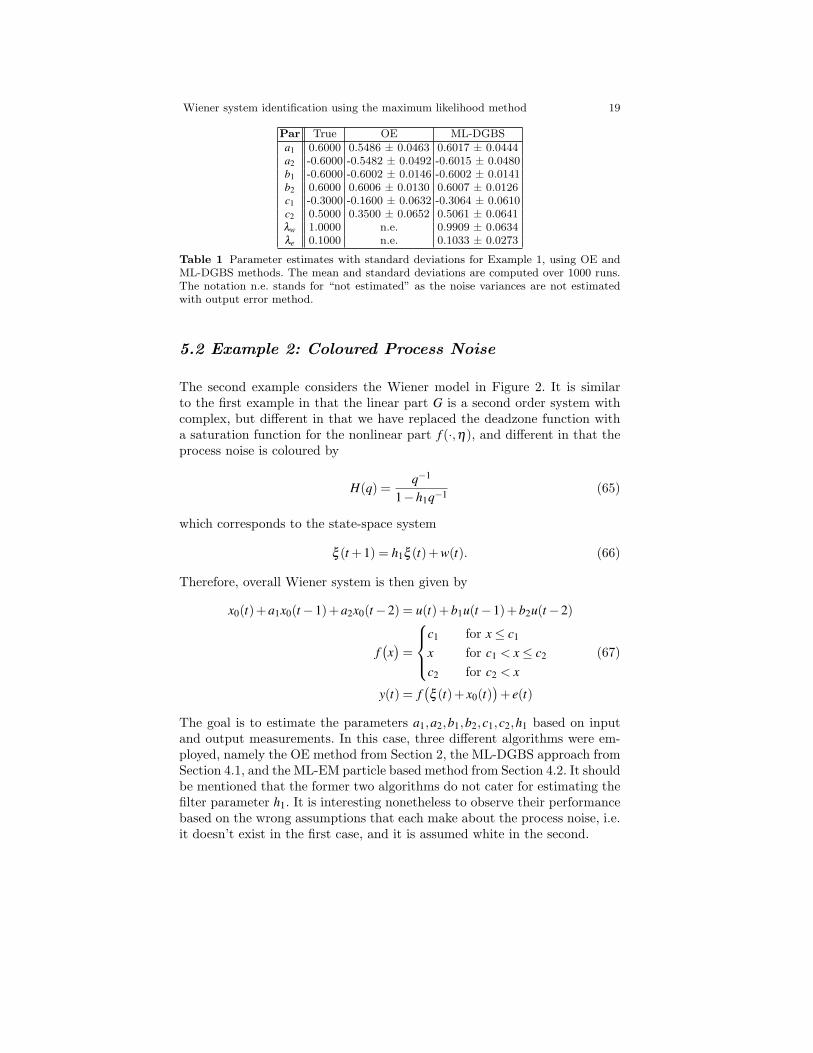
Par True OE ML-DGBSa1 0.6000 0.5486 ± 0.0463 0.6017 ± 0.0444a2 -0.6000 -0.5482 ± 0.0492 -0.6015 ± 0.0480b1 -0.6000 -0.6002 ± 0.0146 -0.6002 ± 0.0141b2 0.6000 0.6006 ± 0.0130 0.6007 ± 0.0126c1 -0.3000 -0.1600 ± 0.0632 -0.3064 ± 0.0610c2 0.5000 0.3500 ± 0.0652 0.5061 ± 0.0641λw 1.0000 n.e. 0.9909 ± 0.0634λe 0.1000 n.e. 0.1033 ± 0.0273

Table 1 Parameter estimates with standard deviations for Example 1, using OE andML-DGBS methods. The mean and standard deviations are computed over 1000 runs.The notation n.e. stands for “not estimated” as the noise variances are not estimatedwith output error method.

5.2 Example 2: Coloured Process Noise

The second example considers the Wiener model in Figure 2. It is similarto the first example in that the linear part G is a second order system withcomplex, but different in that we have replaced the deadzone function witha saturation function for the nonlinear part f (·,η), and different in that theprocess noise is coloured by

H(q) =q−1

1−h1q−1 (65)

which corresponds to the state-space system

ξ (t +1) = h1ξ (t)+w(t). (66)

Therefore, overall Wiener system is then given by

x0(t)+a1x0(t−1)+a2x0(t−2) = u(t)+b1u(t−1)+b2u(t−2)

f(x)

=

c1 for x≤ c1

x for c1 < x≤ c2

c2 for c2 < x

y(t) = f(ξ (t)+ x0(t)

)+ e(t)

(67)

The goal is to estimate the parameters a1,a2,b1,b2,c1,c2,h1 based on inputand output measurements. In this case, three different algorithms were em-ployed, namely the OE method from Section 2, the ML-DGBS approach fromSection 4.1, and the ML-EM particle based method from Section 4.2. It shouldbe mentioned that the former two algorithms do not cater for estimating thefilter parameter h1. It is interesting nonetheless to observe their performancebased on the wrong assumptions that each make about the process noise, i.e.it doesn’t exist in the first case, and it is assumed white in the second.


−1 −0.8 −0.6 −0.4 −0.2 0 0.2 0.4 0.6 0.8 1−1

−0.8

−0.6

−0.4

−0.2

0

0.2

0.4

0.6

0.8

1

x(t)

f(x(

t),η

)

−1 −0.8 −0.6 −0.4 −0.2 0 0.2 0.4 0.6 0.8 1−1

−0.8

−0.6

−0.4

−0.2

0

0.2

0.4

0.6

0.8

1

x(t)

f(x(

t),η

)

Fig. 3 Example 1: The true deadzone function as a thick black line and the 1000estimated deadzones, appearing in grey. Above: OE. Below: ML-DGBS.

As before, we ran a Monte-Carlo simulation with 1000 runs and in eachwe generated a new data set with N = 1000 points. The signals u(t), w(t) ande(t) were generated in the same way as for Example 1. For the EM approach,we used M = 200 particles in approximating Q (see (51)).

The results are summarized in Table 2. It can be observed that the outputerror approach again provides biased estimates of the nonlinearity parame-


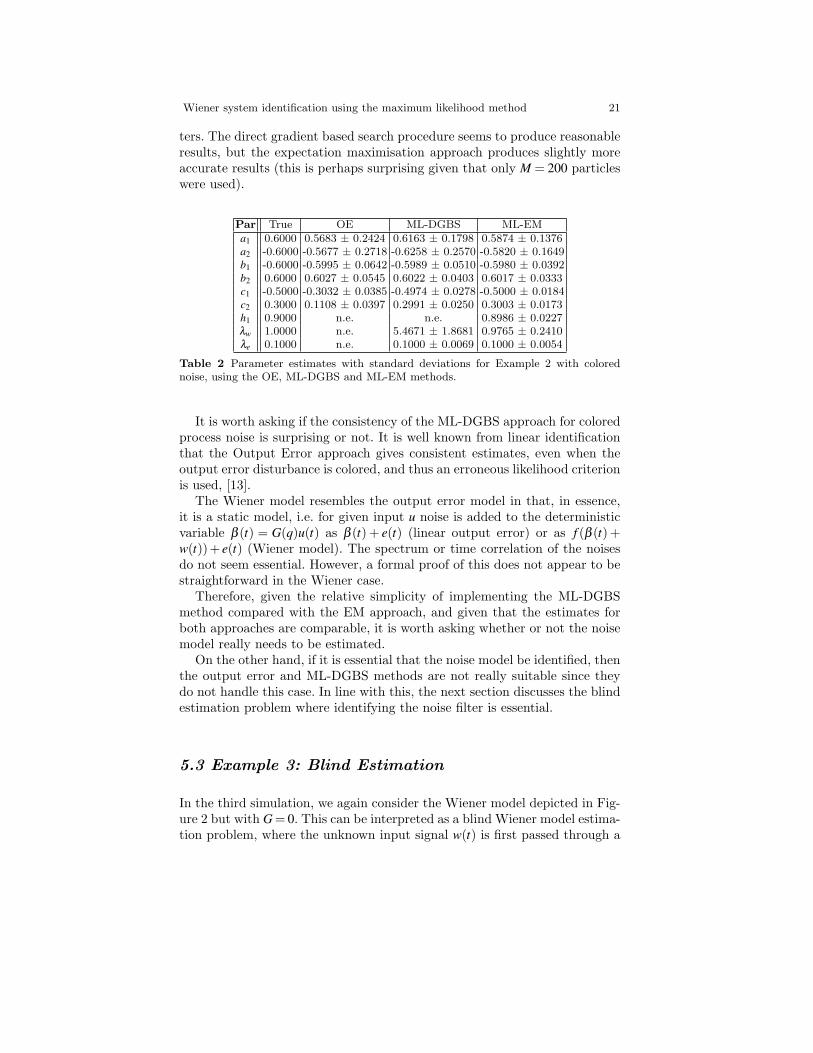
ters. The direct gradient based search procedure seems to produce reasonableresults, but the expectation maximisation approach produces slightly moreaccurate results (this is perhaps surprising given that only M = 200 particleswere used).

Par True OE ML-DGBS ML-EMa1 0.6000 0.5683 ± 0.2424 0.6163 ± 0.1798 0.5874 ± 0.1376a2 -0.6000 -0.5677 ± 0.2718 -0.6258 ± 0.2570 -0.5820 ± 0.1649b1 -0.6000 -0.5995 ± 0.0642 -0.5989 ± 0.0510 -0.5980 ± 0.0392b2 0.6000 0.6027 ± 0.0545 0.6022 ± 0.0403 0.6017 ± 0.0333c1 -0.5000 -0.3032 ± 0.0385 -0.4974 ± 0.0278 -0.5000 ± 0.0184c2 0.3000 0.1108 ± 0.0397 0.2991 ± 0.0250 0.3003 ± 0.0173h1 0.9000 n.e. n.e. 0.8986 ± 0.0227λw 1.0000 n.e. 5.4671 ± 1.8681 0.9765 ± 0.2410λe 0.1000 n.e. 0.1000 ± 0.0069 0.1000 ± 0.0054

Table 2 Parameter estimates with standard deviations for Example 2 with colorednoise, using the OE, ML-DGBS and ML-EM methods.

It is worth asking if the consistency of the ML-DGBS approach for coloredprocess noise is surprising or not. It is well known from linear identificationthat the Output Error approach gives consistent estimates, even when theoutput error disturbance is colored, and thus an erroneous likelihood criterionis used, [13].

The Wiener model resembles the output error model in that, in essence,it is a static model, i.e. for given input u noise is added to the deterministicvariable β (t) = G(q)u(t) as β (t) + e(t) (linear output error) or as f (β (t) +w(t))+ e(t) (Wiener model). The spectrum or time correlation of the noisesdo not seem essential. However, a formal proof of this does not appear to bestraightforward in the Wiener case.

Therefore, given the relative simplicity of implementing the ML-DGBSmethod compared with the EM approach, and given that the estimates forboth approaches are comparable, it is worth asking whether or not the noisemodel really needs to be estimated.

On the other hand, if it is essential that the noise model be identified, thenthe output error and ML-DGBS methods are not really suitable since theydo not handle this case. In line with this, the next section discusses the blindestimation problem where identifying the noise filter is essential.

5.3 Example 3: Blind Estimation

In the third simulation, we again consider the Wiener model depicted in Fig-ure 2 but with G = 0. This can be interpreted as a blind Wiener model estima-tion problem, where the unknown input signal w(t) is first passed through a


filter H(q) and then secondly mapped through a static nonlinearity f . Finally,the measurements are corrupted by the disturbance e(t) to provide y(t).

In particular, we assume as in Example 2 that the process noise is colouredby

H(ϑ ,q) =q−1

1−h1q−1 (68)

and the resulting signal is then mapped through a saturation nonlinearity, sothat the overall Wiener system is given by

y(t) = f(ξ (t)

)+ e(t)

ξ (t +1) = h1ξ (t)+w(t)

f(ξ (t)

)=

c1 for ξ (t)≤ c1

ξ (t) for c1 < ξ (t)≤ c2

c2 for c2 < ξ (t)

(69)

Here we are trying to estimate the parameters h1,c1,c2 and the varianceparameters λw,λe of the process noise w(t) and e(t), respectively. This is tobe done based on the output measurements alone. The EM method describedin Section 4.2 is directly applicable to this case, and was employed here.

As usual, we ran a Monte-Carlo simulation with 1000 runs and in each wegenerated a new data set with N = 1000 points. The signals w(t) and e(t) weregenerated as Gaussian random numbers with variance 1 and 0.1, respectively.In this case, we used only M = 50 particles in approximating Q.

The results are summarized in Table 3. Even with a modest number ofparticles used, M = 50, the estimates are consistent and appear to be accurate.

Par True ML-EMb2 0.9000 0.8995 ± 0.0237c1 -0.5000 -0.4967 ± 0.0204c2 0.3000 0.2968 ± 0.0193λw 1.0000 1.0293 ± 0.1744λe 0.1000 0.1019 ± 0.0063

Table 3 Parameter estimates with standard deviations for Example 3, using the EMmethod.

6 Conclusion

The dominant approach for estimating Wiener models is to parametrize thelinear and nonlinear parts and then minimise, with respect to these param-eters, the squared error between the measured output and a simulated one


from the Wiener model. This approach implicitly assumes that no processnoise is present. It was confirmed that this leads to biased estimates if theassumption is wrong.

To overcome this problem, the chapter presents two algorithms for pro-viding maximum likelihood estimates of Wiener models that include bothprocess and measurement noise. The first is based on the assumption thatthe process noise is white, and the second assumes that the process noisehas been coloured by a linear filter. In the latter case, the likelihood functioninvolves the evaluation of a high dimension integral, which is not tractableusing traditional numerical integration techniques.

Motivated by this, the chapter casts the Wiener model in the form of anonlinear state-space model, which is directly amenable to a recently devel-oped Expectation Maximisation algorithm. Of vital importance is that theexpectation step can be approximated using sequential importance resam-pling (or particle) methods, which are easily implemented using standarddesktop computing. This approach was profiled for the case of coloured pro-cess noise with very promising results.

Finally, the case of blind Wiener model estimation can be directly handledusing the expectation maximisation method presented here. The efficacy ofthis method was demonstrated via a simulation example.

References

1. Er-Wei Bai. Frequency domain identification of Wiener models. Automatica,39(9):1521–1530, 2003.

2. S. A. Billings. Identification of non-linear systems - a survey. IEE Proc. D, 127:272–285, 1980.

3. Stephen Boyd and Leon O. Chua. Fading memory and the problem of approximat-ing nonlinear operators with Volterra series. IEEE Transactions on Circuits andSystems, CAS-32(11):1150–1161, November 1985.

4. J. E. Dennis, Jr and R. B. Schnabel. Numerical Methods for Unconstrained Op-timization and Nonlinear Equations. Prentice-Hall, Englewood Cliffs, New Jersey,USA, 1983.

5. S. Gibson and B. Ninness. Robust maximum-likelihood estimation of multivariabledynamic systems. Automatica, 41(10):1667–1682, 2005.

6. N. J. Gordon, D. J. Salmond, and A. F. M. Smith. A novel approach tononlinear/non-Gaussian Bayesian state estimation. In IEE Proceedings on Radarand Signal Processing, volume 140, pages 107–113, 1993.

7. Anna Hagenblad and Lennart Ljung. Maximum likelihood estimation of wienermodels. In Proc. 39:th IEEE Conf. on Decision and Control, pages 2417–2418,Sydney, Australia, Dec 2000.

8. Anna Hagenblad, Lennart Ljung, and Adrian Wills. Maximum likelihood identifi-cation of wiener models. Automatica, 44(11):2697–2705, November 2008.

9. Kenneth Hsu, Tyrone Vincent, and Kameshwar Poolla. A kernel based approach tostructured nonlinear system identification part i: Algorithms, part ii: Convergenceand consistency. In Proc. IFAC Symposium on System Identification, Newcastle,March 2006.


10. I. W. Hunter and M. J. Korenberg. The identification of nonlinear biological systems:Wiener and Hammerstein cascade models. Biological Cybernetics, 55:135–144, 1986.

11. A. Kalafatis, N. Arifin, L. Wang, and W. R. Cluett. A new approach to the identifi-cation of pH processes based on the Wiener model. Chemical Engineering Science,50(23):3693–3701, 1995.

12. L. Ljung, R. Singh, Q. Zhang, P. Lindskog, and A. Juditski. Developments inMathworks system identification toolbox. In Proc. 15th IFAC Symposium on SystemIdentification, Saint-Malo, France, July 2009.

13. Lennart Ljung. System Identification, Theory for the User. Prentice Hall, EnglewoodCliffs, New Jersey, USA, second edition, 1999.

14. G. McLachlan and T. Krishnan. The EM Algorithm and Extensions (2nd Edition).John Wiley and Sons, 2008.

15. J. Nocedal and S. J. Wright. Numerical Optimization, Second Edition. Springer-Verlag, New York, 2006.

16. W. H. Press, S. A. Teukolsky, W. A. Vetterling, and B. P. Fannery. NumericalRecipes in C, the Art of Scientific Computing, Second Edition. Cambridge UniversityPress, Cambridge, 1992.

17. Thomas Schön, Adrian Wills, and Brett Ninness. System identification of nonlinearstate-space models. Automatica (provisionally accepted), November 2009.

18. J. Schoukens, J. G. Nemeth, P. Crama, Y. Rolain, and R. Pintelon. Fast approximateidentification of nonlinear systems. Automatica, 39(7):1267–1274, 2003. July.

19. L. Vanbaylen, R. Pintelon, and P. de Groen. Blind maximum likelihood identificationof wiener systems with measurement noise. In Proc. 15th IFAC Symposium onSystem Identification, pages 1686–1691, Saint-Malo, France, July 2009.

20. L. Vanbaylen, R. Pintelon, and J. Schoukens. Blind maximum-likelihood identifica-tion of wiener systems. IEEE Transactions on Signal Processing, 57(8):3017–3029,August 2009.

21. David Westwick and Michel Verhaegen. Identifying MIMO Wiener systems usingsubspace model identification methods. Signal Processing, 52:235–258, 1996.

22. Torbjörn Wigren. Recursive prediction error identification using the nonlinearWiener model. Automatica, 29(4):1011–1025, 1993.

23. A. G. Wills, A. J. Mills, and B. Ninness. A matlab software environment for systemidentification. In Proc, 15th IFAC Symposium on System Identification, Saint-Malo,France, July 2009.

24. Yucai Zhu. Distillation column identification for control using Wiener model. In1999 American Control Conference, Hyatt Regency San Diego, California, USA,June 1999.

Avdelning, Institution

Division, Department

Division of Automatic ControlDepartment of Electrical Engineering

Datum

Date

2010-12-20

Språk

Language

� Svenska/Swedish

� Engelska/English

�

�

Rapporttyp

Report category

� Licentiatavhandling

� Examensarbete

� C-uppsats

� D-uppsats

� Övrig rapport

�

�

URL för elektronisk version


ISBN

�

ISRN

�

Serietitel och serienummer

Title of series, numberingISSN

1400-3902

LiTH-ISY-R-2990

Titel

TitleWiener system identi�cation using the maximum likelihood method

Författare

AuthorAdrian Wills, Lennart Ljung

Sammanfattning

Abstract

The Wiener model is a block oriented model where a linear dynamic system block is fol-lowed by a static nonlinearity block. The dominant method to estimate these componentshas been to minimize the error between the simulated and the measured outputs. This isknown to lead to biased estimates if disturbances other than measurement noise are present.For the case of more general disturbances we present Maximum Likelihood expressions andprovide algorithms for maximising them. This includes the case where disturbances may becoloured and as a consequence we can handle blind estimation of Wiener models. This case isaccommodated by using the Expectation-Maximisation algorithm in combination with parti-cles methods. Comparisons between the new algorithms and the dominant approach con�rmthat the new method is unbiased and also has superior accuracy.

Nyckelord

Keywords System Identi�cation, Nonlinear models, maxximum likelihood, Wiener models


wiener system identification using the maximum likelihood

Documents